Generation of Light Fields with Controlled Non-Uniform Elliptical Polarization When Focusing on Structured Laser Beams

Abstract

We study the sharp focusing of the input structured light field that has a non-uniform elliptical polarization: the parameters of the ellipse depend on the position in the input plane (we limited ourselves to the dependence only on the angular variable). Two types of non-uniformity were considered. The first type corresponds to the situation when the semi-axes of the polarization ellipse are fixed while the slope of the major semi-axis changes. The second type is determined by the situation when the slope of the major semi-axis of the polarization ellipse is constant, and the ratio between the semi-axis changes (we limited ourselves to the trigonometric dependence of this ratio on the polar angle). Theoretical and numerical calculations show that in the case of the first type of non-uniformity, if the tilt angle is a multiple of the polar angle with an integer coefficient, then the intensity distribution has rotational symmetry, and the energy flow is radially symmetric and has the negative direction near the optical axis. In this second case, the intensity symmetry is not very pronounced, but with an odd dependence of the ratio of the semi-axes of the polarization ellipse, the focused field at each point has a local linear polarization, despite the rather complex form of the input field. In addition, we investigate the distribution of the longitudinal component of the Poynting vector. The obtained results may be used for the formation of focused light fields with the desired distributions of polarization, Poynting vector density, or spin angular momentum density in the field of laser manipulation and laser matter interaction.

1. Introduction

The development of various techniques and devices for modulating such characteristics of laser radiation as its amplitude, phase, and polarization distributions [1,2,3] led to the widespread use of structured laser beams in various areas of science and technology. Structured laser beams are indispensable in such areas as advanced optical trapping and manipulation of nano- and micro-objects in various media, mode division multiplexing (MDM) optical communication systems, quantum communication, optical microscopy, laser material processing, and many others [4,5,6,7,8,9,10,11,12,13,14,15]. The most popular approaches for the shaping of structured light are the use of diffractive optical elements (DOEs), metasurfaces, structured screens, or spatial light modulators (SLMs) [16,17,18,19,20,21,22,23,24,25]. These elements and devices can be used to control individual characteristics of laser beams or to control some of them in parallel—for example, amplitude and phase or phase and polarization. Recently, increasingly complex combinations of phase distributions [26,27,28,29,30] and hybrid polarization states [31,32,33,34,35,36] have been used to generate structured laser beams in order to increase the number of degrees of freedom, which can be used, for example, in MDM optical communication or high-performance precision laser processing of materials [37,38,39,40,41,42,43]. It should be noted that the combination of a vortex phase singularity and cylindrical polarization states of various orders are very popular for this [10,31,34,37,40]. This is due both to the influence of this type of polarization on the amplification of the longitudinal component of the electric field during sharp focusing [10,44,45] and to the specifics of the effect of such laser radiation on matter [46,47,48,49,50]. In addition, the interaction of a phase singularity with a cylindrical polarization type is also a reason for various effects [51,52,53,54]. For example, the high numerical aperture (NA) focusing leads to the conversion of cylindrically polarized laser beams from a radial to an azimuthal polarization, or vice versa, by introducing a higher-order vortex phase singularity [53].

However, not only cylindrical polarization but also other types of inhomogeneous polarization, including hybrid polarization states [55], are also increasingly attracting the attention of researchers [14,32,35,40,56,57], since they can be used for the generation of complex distributions of spin angular momentum (SAM) [14,58], the implementation of spin-orbit interaction [40,59,60,61,62,63,64], and generation of polarization singularities of various types [65,66,67,68,69]. Hybrid polarized vector fields have completely different properties from the reported scalar and vector fields.

Elliptical polarization is the most general type of polarization that can be characterized by the polarization ellipse, which can be specified by its ellipticity and orientation angle. In this work, we investigate the possibilities of controlling these parameters of elliptical polarization at different points of the generated hybrid polarized light field through high-NA focusing laser fields with the predetermined transverse components of the electromagnetic field. Such control provides tools for the generation of structured light fields with the desired distribution of Poynting vector density or spin angular momentum density. Moreover, light fields with non-uniform distribution of polarization are widely used for the fabrication of laser-induced periodic surface structures (LIPSSs) with unconventional morphology [20,48,70]. Such structures can provide basic units that replicate over larger areas allowing fabricating complex surfaces with novel or extended functionality. The proposed approach for the generation of non-uniform elliptical polarization is based on the use of high-NA focused structured laser fields. This allows one to control such parameters of the generated polarization distributions as the ellipticity of the formed polarization ellipse, its orientation, and the rotation direction of the polarization vector at each point of the focused light field.

2. Theoretical Background

With elliptical polarization, the electric field vector describes the contour of an ellipse (see Figure 1). The complex amplitudes of the components of the elliptically polarized field (eliminating the time-space component ωt − kz) are described in terms of the Jones vector as follows:

$$\left(\begin{array}{c}{E}_x\\ E_y\end{array}\right)=\left(\begin{array}{c}{A}_x\exp (i{\delta }_x)\\ A_y\exp (i{\delta }_y)\end{array}\right)\simeq \left(\begin{array}{c}{A}_x\\ A_y\exp (i\Delta )\end{array}\right),$$

(1)

where A_x, A_y are amplitudes and δ_x, δ_y are phases of corresponding components, and Δ = δ_y − δ_x.

The polarization ellipse is also defined by the orientation or tilt angle α (0 ≤ α ≤ π):

$$\tan \left(2\mathsf{\alpha }\right)=\frac{2A_x{A}_y\cos \left(\Delta \right)}{A_x{}^2-A_y{}^2}.$$

(2)

Next, in this work, we will be interested in the following parameters:

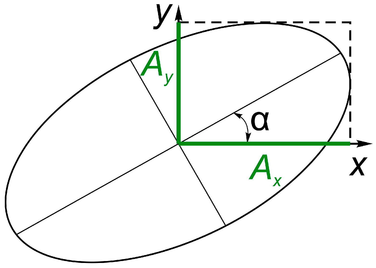
• the ratio of the semi-axes (which depends on amplitudes A_x and A_y);
• inclination of the semi-major axis (i.e., angle α);
• vector rotation direction.

In order to control the parameters of the polarization ellipse in different regions of the focal plane, as a rule, it is necessary to consider the situation in which the initial field also has a non-uniform polarization.

To calculate the components of the electric and magnetic field vectors in the focal region, we use the following formulas [71,72,73]:

$$\begin{array}{l}\left[\begin{array}{c}E(r,\upsilon ,z)\\ H(r,\upsilon ,z)\end{array}\right]=\\ =-\frac{if}{\lambda }{\displaystyle \underset{0}{\overset{\Theta }{\int }}{\displaystyle \underset{0}{\overset{2\pi }{\int }}\left[\begin{array}{c}{P}_E(\mathsf{\theta },\mathsf{\phi })\\ P_H(\mathsf{\theta },\mathsf{\phi })\end{array}\right]E_0(\mathsf{\theta },\mathsf{\phi })T(\mathsf{\theta })\exp \left[ik(r\sin \mathsf{\theta }\cos (\mathsf{\phi }-\upsilon )+z\cos \mathsf{\theta })\right]}}\sin \mathsf{\theta }d\mathsf{\theta }d\mathsf{\phi },\end{array}$$

(3)

where

$$P_E(\mathsf{\theta },\mathsf{\phi })=\left[\begin{array}{cc}A(\mathsf{\theta },\mathsf{\phi })& C(\mathsf{\theta },\mathsf{\phi })\\ C(\mathsf{\theta },\mathsf{\phi })& B(\mathsf{\theta },\mathsf{\phi })\\ -D(\mathsf{\theta },\mathsf{\phi })& -E(\mathsf{\theta },\mathsf{\phi })\end{array}\right],\hspace{0.17em}\hspace{0.17em}\hspace{0.17em}\hspace{0.17em}\hspace{0.17em}\hspace{0.17em}\hspace{0.17em}{P}_H(\mathsf{\theta },\mathsf{\phi })=\left[\begin{array}{cc}C(\mathsf{\theta },\mathsf{\phi })& -A(\mathsf{\theta },\mathsf{\phi })\\ B(\mathsf{\theta },\mathsf{\phi })& -C(\mathsf{\theta },\mathsf{\phi })\\ -E(\mathsf{\theta },\mathsf{\phi })& D(\mathsf{\theta },\mathsf{\phi })\end{array}\right],$$

(4)

$$\begin{array}{l}A(\mathsf{\theta },\mathsf{\phi })=1+{\cos }^2\mathsf{\phi }(\cos \mathsf{\theta }-1),\hspace{1em}B(\mathsf{\theta },\mathsf{\phi })=1+{\sin }^2\mathsf{\phi }(\cos \mathsf{\theta }-1),\\ C(\mathsf{\theta },\mathsf{\phi })=\sin \mathsf{\phi }\cos \mathsf{\phi }(\cos \mathsf{\theta }-1),\hspace{1em}D(\mathsf{\theta },\mathsf{\phi })=\cos \mathsf{\phi }\sin \mathsf{\theta },\hspace{1em}E(\mathsf{\theta },\mathsf{\phi })=\sin \mathsf{\phi }\sin \mathsf{\theta }.\end{array}$$

(5)

Here, (r, υ, z) are the cylindrical coordinates in the focal region, (θ, φ) are the spherical angular coordinates of the focusing system’s output pupil (see Figure 2), Θ is the maximum value of the azimuthal angle θ related to the system’s numerical aperture NA = sinΘ, k = 2π/λ is the wavenumber and λ is the radiation wavelength, f is a focal length of an optical system, T(θ) is the apodization function; $E_0(\mathsf{\theta },\mathsf{\phi })=\left(\begin{array}{c}{E}_{0x}(\mathsf{\theta },\mathsf{\phi })\\ E_{0y}(\mathsf{\theta },\mathsf{\phi })\end{array}\right)$ is the transverse components of the electric vector of the input field. The focal plane corresponds to z = 0.

We also consider the Umov-Poynting vector:

$$\mathit{S}=\frac{c}{8\pi }\left({\mathit{E}}^{*}\times \mathit{H}\right),$$

(6)

in particular, its longitudinal component, which, up to a constant coefficient, is equal to:

$$S_z=\left(E_x^{*}{H}_y-E_y^{*}{H}_x\right).$$

(7)

In the classical definition, one needs to take the real part of Equation (6) or Equation (7), but we regard the full values since the imaginary part may also have a physical meaning [74,75,76].

3. Results

In this section, we analyze analytically and illustrate numerically some special cases of focusing vector fields with inhomogeneous elliptical polarization. Numerical simulation was performed using Equations (3)–(5) without any approximations under full aperture conditions at NA = 0.99 (Θ ≈ 82°), $T(\mathsf{\theta })=\sqrt{\cos \mathsf{\theta }}$. The radius of the input fields is 100λ, and the output field size is 2λ × 2λ.

3.1. Variable Tilt Angle of the Polarization Ellipse

First, we consider the possibility of controlling the angle of inclination of the ellipse α. We fix the amplitudes A_x and A_y and consider an arbitrary function for a variable slope angle α(θ, φ). Then, the components of the electric field are expressed by the following formulas:

$$\begin{array}{l}{E}_{0x}\left(\mathsf{\theta },\mathsf{\phi }\right)=F\left(\mathsf{\theta }\right)\cdot \left\{A_x\cos \left[\alpha \left(\mathsf{\theta },\mathsf{\phi }\right)\right]+i{A}_y\sin \left[\alpha \left(\mathsf{\theta },\mathsf{\phi }\right)\right]\right\},\\ E_{0y}\left(\mathsf{\theta },\mathsf{\phi }\right)=F\left(\mathsf{\theta }\right)\cdot \left\{A_x\sin \left[\alpha \left(\mathsf{\theta },\mathsf{\phi }\right)\right]-i{A}_y\cos \left[\alpha \left(\mathsf{\theta },\mathsf{\phi }\right)\right]\right\},\end{array}$$

(8)

where F(θ) is an arbitrary function depending on the azimuth angle θ.

Let us consider special examples of the dependence α(θ, φ), only on the polar angle φ.

3.1.1. The Tilt Angle of the Polarization Ellipse Is Equal to the Polar Angle

First, we consider the simplest and visually symmetrical case when the slope angle is equal to the direction angle of the radius vector:

$$\alpha (\mathsf{\theta },\mathsf{\phi })=\alpha (\mathsf{\phi })=\mathsf{\phi }.$$

(9)

Substituting this expression in Equation (8), we obtain the expression for the initial field:

$$\begin{array}{l}{E}_{0x}\left(\mathsf{\theta },\mathsf{\phi }\right)=F(\mathsf{\theta })\cdot \left\{A_x\cos \mathsf{\phi }+i{A}_y\sin \mathsf{\phi }\right\},\\ E_{0y}\left(\mathsf{\theta },\mathsf{\phi }\right)=F(\mathsf{\theta })\cdot \left\{A_x\sin \mathsf{\phi }-i{A}_y\cos \mathsf{\phi }\right\}.\end{array}$$

(10)

The field in Equation (10) can be represented in another form:

$$E_0\left(\mathsf{\theta },\mathsf{\phi }\right)=F(\mathsf{\theta })\cdot \left\{A_x\left(\begin{array}{l}\cos \mathsf{\phi }\\ \sin \mathsf{\phi }\end{array}\right)-i{A}_y\left(\begin{array}{l}-\sin \mathsf{\phi }\\ \cos \mathsf{\phi }\end{array}\right)\right\}$$

(11)

This is a combination of radial and azimuthal polarizations with different weights, with one of the weights real and the other purely imaginary.

Let us calculate the field components in the focal plane if the field in the initial plane is given by Equation (10). To do this, we use Equations (3)–(5):

$$\left[\begin{array}{l}{E}_x\\ E_y\\ E_z\end{array}\right]=-\frac{if}{\lambda }{\displaystyle \underset{0}{\overset{\Theta }{\int }}T(\mathsf{\theta })F(\mathsf{\theta })\sin \mathsf{\theta }\left[\begin{array}{l}{A}_x\cos \mathsf{\theta }\cdot S_{1,0}+i{A}_y\cdot S_{0,1}\\ A_x\cos \mathsf{\theta }\cdot S_{0,1}-i{A}_y\cdot S_{1,0}\\ -A_x\sin \mathsf{\theta }\cdot S_{0,0}\end{array}\right]d\mathsf{\theta }},$$

(12)

$$\left[\begin{array}{l}{H}_x\\ H_y\\ H_z\end{array}\right]=-\frac{if}{\lambda }{\displaystyle \underset{0}{\overset{\Theta }{\int }}T(\mathsf{\theta })F(\mathsf{\theta })\sin \mathsf{\theta }\left[\begin{array}{l}-A_x\cdot S_{0,1}+i{A}_y\cos \mathsf{\theta }\cdot S_{1,0}\\ A_x\cdot S_{1,0}+i{A}_y\cos \mathsf{\theta }\cdot S_{0,1}\\ -i{A}_y\sin \mathsf{\theta }\cdot S_{0,0}\end{array}\right]d\mathsf{\theta }},$$

(13)

where we use the following notation:

$$S_{p,q}={\displaystyle \underset{0}{\overset{2\pi }{\int }}{\cos }^p\mathsf{\phi }\cdot {\sin }^q\mathsf{\phi }\cdot \exp \left(ia\cos (\mathsf{\phi }-\upsilon )\right)d\mathsf{\phi },\hspace{1em}a=kr\sin \mathsf{\theta }}$$

(14)

We give explicit expressions for S_p,q for p + q ≤ 3 (these will be needed here and below):

$$\begin{array}{l}{S}_{0,0}=2\pi J_0(a),\\ S_{1,0}=\cos \upsilon \cdot 2\pi i{J}_1(a),\hspace{1em}{S}_{0,1}=\sin \upsilon \cdot 2\pi i{J}_1(a),\\ S_{2,0}=\pi J_0(a)-\cos 2\upsilon \cdot \pi J_2(a),\hspace{1em}{S}_{0,2}=\pi J_0(a)+\cos 2\upsilon \cdot \pi J_2(a),\\ S_{1,1}=-\sin 2\upsilon \cdot \pi J_2(a),\\ S_{3,0}=\cos \upsilon \cdot 1.5\pi i{J}_1(a)-\cos 3\upsilon \cdot 0.5\pi i{J}_3(a),\hspace{1em}{S}_{0,3}=\sin \upsilon \cdot 1.5\pi i{J}_1(a)+\sin 3\upsilon \cdot 0.5\pi i{J}_3(a),\\ S_{2,1}=\sin \upsilon \cdot 0.5\pi i{J}_1(a)-\sin 3\upsilon \cdot 0.5\pi i{J}_3(a),\hspace{1em}{S}_{1,2}=\cos \upsilon \cdot 0.5\pi i{J}_1(a)+\cos 3\upsilon \cdot 0.5\pi i{J}_3(a).\end{array}$$

(15)

Explicit analytical expressions for Equations (12) and (13) can be obtained approximately in the case of a narrow annular aperture [44,77,78], i.e., when $F(\mathsf{\theta })=\left\{\begin{array}{c}1,\hspace{0.17em}\hspace{0.17em}{\mathsf{\theta }}_0-\Delta /2\le \mathsf{\theta }\le {\mathsf{\theta }}_0+\Delta /2,\\ 0,\hspace{0.17em}\hspace{0.17em}else.\end{array}\right.$.

Then for the components of the electric and magnetic vectors we can write:

$$\begin{array}{l}{E}_x=kf\cdot \Delta \cdot T({\mathsf{\theta }}_0)F({\mathsf{\theta }}_0)\sin {\mathsf{\theta }}_0{J}_1(a)\left(A_x\cos {\mathsf{\theta }}_0\cos \upsilon +i{A}_y\sin \upsilon \right),\\ E_y=kf\cdot \Delta \cdot T({\mathsf{\theta }}_0)F({\mathsf{\theta }}_0)\sin {\mathsf{\theta }}_0{J}_1(a)\left(A_x\cos {\mathsf{\theta }}_0\sin \upsilon -i{A}_y\cos \upsilon \right),\\ E_z=kf\cdot \Delta \cdot T({\mathsf{\theta }}_0)F({\mathsf{\theta }}_0)\sin {\mathsf{\theta }}_0{J}_0(a)\left(i{A}_x\sin {\mathsf{\theta }}_0\right).\end{array}$$

(16)

$$\begin{array}{l}{H}_x=kf\cdot \Delta \cdot T({\mathsf{\theta }}_0)F({\mathsf{\theta }}_0)\sin {\mathsf{\theta }}_0{J}_1(a)\left(-A_x\sin \upsilon +i{A}_y\cos {\mathsf{\theta }}_0\cos \upsilon \right),\\ H_y=kf\cdot \Delta \cdot T({\mathsf{\theta }}_0)F({\mathsf{\theta }}_0)\sin {\mathsf{\theta }}_0{J}_1(a)\left(A_x\cos \upsilon +i{A}_y\cos {\mathsf{\theta }}_0\sin \upsilon \right),\\ H_z=kf\cdot \Delta \cdot T({\mathsf{\theta }}_0)F({\mathsf{\theta }}_0)\sin {\mathsf{\theta }}_0{J}_0(a)\left(-A_y\sin {\mathsf{\theta }}_0\right).\end{array}$$

(17)

Note that the longitudinal component of the electric field is purely imaginary, while that of the magnetic field is real.

Using the resulting expressions, we can find other characteristics. In particular, the total intensity is:

$$I_{tot}={\left(kf\cdot \Delta \cdot T({\mathsf{\theta }}_0)F({\mathsf{\theta }}_0)\sin {\mathsf{\theta }}_0\right)}^2\left[J_0^2(a)\cdot A_x^2{\sin }^2{\mathsf{\theta }}_0+J_1^2(a)\left(A_x^2{\cos }^2{\mathsf{\theta }}_0+A_y^2\right)\right],$$

(18)

and the longitudinal component of the Umov-Poynting vector:

$$S_z={\left(kf\cdot \Delta \cdot T({\mathsf{\theta }}_0)F({\mathsf{\theta }}_0)\sin {\mathsf{\theta }}_0\right)}^2\left[J_1^2(a)\cos {\mathsf{\theta }}_0\left(A_x^2+A_y^2\right)\right].$$

(19)

Note that for the considered case α(φ) = φ, the intensity I in Equation (18) depends on the ratio A_x and A_y, but $S_z$ in Equation (19) does not have such a dependence and takes everywhere real positive values.

Figure 3 shows the calculated results of the formation of fields with inhomogeneous elliptical polarization (red color corresponds to the x-component, green color is for the y-component, and blue color is for the z-component) at α(φ) = φ.

As can be seen from the results shown in Figure 3, the equality of the amplitudes A_x = A_y provides a completely uniform distribution of the polarization of the input field; however, in the focal plane, the polarization state becomes inhomogeneous (Figure 3a,b). The inequality A_x ≠ A_y leads to inhomogeneity of the polarization distribution both in the input and in the focused field. In the example A_x > A_y (Figure 3c,d), according to Equation (16), there is an increase in the proportion of the longitudinal component.

The formation of fields close to those shown in Figure 3 was considered in Ref. [33] on the basis of a combination of structured beams with left and right circular polarization, as well as in Ref. [20] on the basis of a modification of the radially polarized field.

Next, we consider initial fields with a more complex polarization structure.

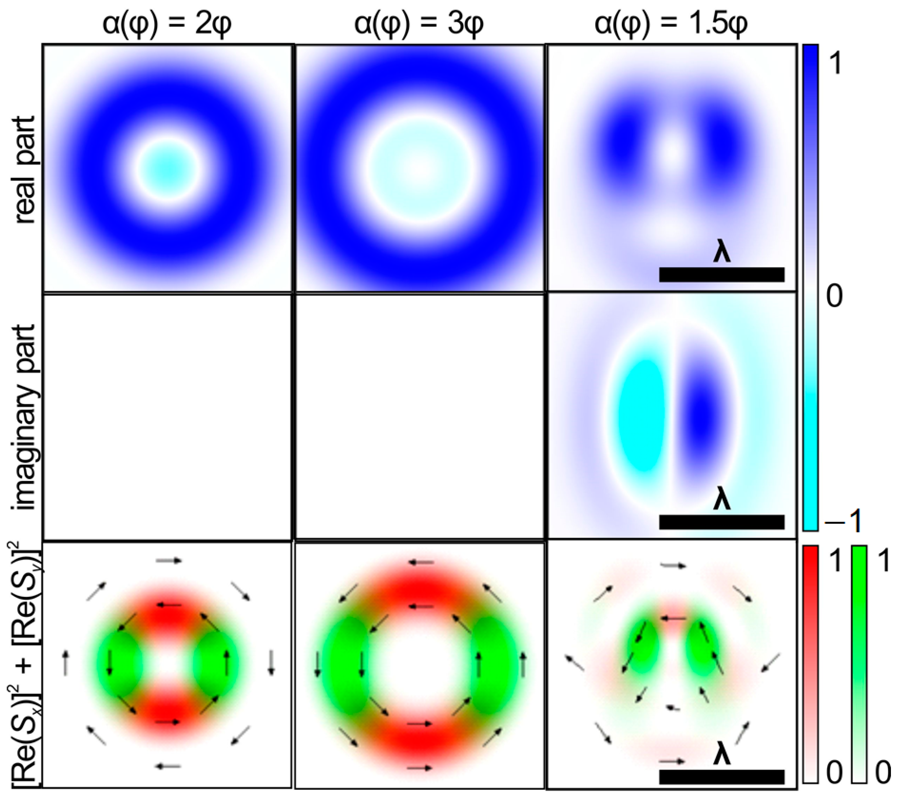
3.1.2. The Tilt Angle of the Polarization Ellipse Is a Multiple of the Polar Angle

Let us consider a multiple increase in the angle of inclination of the ellipse, i.e., instead of expression (9), a more general one:

$$\alpha (\mathsf{\phi })=p\mathsf{\phi }.$$

(20)

In the case when p is an integer, one can obtain explicit analytical expressions for the field in the focal plane, similar to those given in the previous section.

For further calculations, Equation (12) can be conveniently written as:

$$\left[\begin{array}{l}{E}_x\\ E_y\\ E_z\end{array}\right]=-\frac{if}{\lambda }{\displaystyle \underset{0}{\overset{\Theta }{\int }}T(\mathsf{\theta })F(\mathsf{\theta })\sin \mathsf{\theta }\left[\begin{array}{l}{\widehat{E}}_x\\ {\widehat{E}}_y\\ {\widehat{E}}_z\end{array}\right]d\mathsf{\theta }}.$$

(21)

Using the basic Equations (4) and (5) and the following formula:

$${\displaystyle \underset{0}{\overset{2\pi }{\int }}\exp \left[ia\cos (\mathsf{\phi }-\upsilon )\right]\left\{\begin{array}{l}\cos m\mathsf{\phi }\\ \sin m\mathsf{\phi }\end{array}\right\}d\mathsf{\phi }}=\left\{\begin{array}{l}\cos m\upsilon \\ \sin m\upsilon \end{array}\right\}2\pi i^m{J}_m(a),$$

(22)

we obtain the following expressions included in Equation (21):

$$\begin{array}{l}{\widehat{E}}_x=\pi i^p\left[\begin{array}{l}(1+\cos \mathsf{\theta })J_p(a)\cdot \left(A_x\cos p\upsilon +i{A}_y\sin p\upsilon \right)+\\ +(1-\cos \mathsf{\theta })J_{p-2}(a)\cdot \left(A_x\cos (p-2)\upsilon +i{A}_y\sin (p-2)\upsilon \right)\end{array}\right],\\ {\widehat{E}}_y=\pi i^p\left[\begin{array}{l}(1+\cos \mathsf{\theta })J_p(a)\cdot \left(A_x\sin p\upsilon -i{A}_y\cos p\upsilon \right)-\\ -(1-\cos \mathsf{\theta })J_{p-2}(a)\cdot \left(A_x\sin (p-2)\upsilon -i{A}_y\cos (p-2)\upsilon \right)\end{array}\right],\\ {\widehat{E}}_z=\sin \mathsf{\theta }\cdot 2\pi i^{p+1}{J}_{p-1}(a)\cdot \left(A_x\cos (p-1)\upsilon +i{A}_y\sin (p-1)\upsilon \right).\end{array}$$

(23)

Note that for p = 1 Equation (23) will correspond to Equations (12) and (15). Assuming a narrow annular aperture with a medium radius ${\mathsf{\theta }}_0$, one can obtain an explicit expression for the total intensity ($a=kr\sin {\mathsf{\theta }}_0$):

$$\begin{array}{l}{I}_{tot}\propto 4{\pi }^2{\sin }^2{\mathsf{\theta }}_0\cdot J_{p-1}^2(a)\cdot \left(A_x^2{\cos }^2(p-1)\upsilon +A_y^2{\sin }^2(p-1)\upsilon \right)+\\ +{\pi }^2\cdot \left[\begin{array}{l}{(1+\cos {\mathsf{\theta }}_0)}^2{J}_p^2(a)\cdot \left(A_x^2+A_y^2\right)+{(1-\cos {\mathsf{\theta }}_0)}^2{J}_{p-2}^2(a)\cdot \left(A_x^2+A_y^2\right)+\\ +2{\sin }^2{\mathsf{\theta }}_0\cdot J_p(a)J_{p-2}(a)\cdot \left(A_x^2-A_y^2\right)\cos (2p-2)\upsilon \end{array}\right].\end{array}$$

(24)

In addition, for p = 1, Equation (24) corresponds to Equation (18).

Note that for p ≠ 1, Equation (24) has terms that depend on the polar angle υ (for p = 1, there is axial symmetry), which is more clearly seen if we rewrite Equation (24) in the following form:

$$\begin{array}{l}{I}_{tot}\propto {\pi }^2\left[{(1+\cos {\mathsf{\theta }}_0)}^2{J}_p^2(a)+{(1-\cos {\mathsf{\theta }}_0)}^2{J}_{p-2}^2(a)+2{\sin }^2{\mathsf{\theta }}_0\cdot J_{p-1}^2(a)\right]\cdot \left(A_x^2+A_y^2\right)+\\ +2{\pi }^2{\sin }^2{\mathsf{\theta }}_0\cdot \left(J_{p-1}^2(a)+J_p(a)J_{p-2}(a)\right)\left(A_x^2-A_y^2\right)\cos \left[(2p-2)\upsilon \right].\end{array}$$

(25)

As can be seen from Equation (25), the dependence on the angle in the intensity of the focused field disappears when A_x = A_y. The inequality A_x ≠ A_y leads to a situation when the intensity will have (2p − 2) maxima and (2p − 2) minima (except for circles where $J_{p-1}^2(a)+J_p(a)J_{p-2}(a)=0$).

If p is a non-integer, it is difficult to represent the generated field in an analytical form, but it is quite possible to perform a simulation. Figure 4 and Figure 5 show calculations of the formation of fields with inhomogeneous elliptical polarization at α(φ) = pφ for integer values p = 2, 3, and Figure 6 shows results for the fractional value p = 0.5.

Figure 4 and Figure 5 clearly show what happens when the amplitude ratio changes from A_x = 2A_y to A_x = 0.5A_y. When p = 2, there is practically a rotation of the entire distribution in the focal plane by 90 degrees (compare the last two lines in Figure 4). The case p = 2 is a special one since in this case some terms in Equation (23) are set to zero, so the structure is pretty simple. At p = 3, only the intensity distribution rotates by 45 degrees, and the polarization state changes in a more complex way (compare the last two lines in Figure 5).

In the general case, in accordance with Equation (25), there will be a rotation of the intensity by 90/(p − 1) degrees, and the polarization transformation will be quite complex.

Figure 6 shows an example with a fractional p value. Since p = 1.5 is half-integer, the input field still has an integer (third-order) rotational symmetry. In contrast to the integer p, when the amplitude ratio changes from A_x = 2A_y to A_x = 0.5A_y, a qualitative change occurs not only in the distribution of the polarization state but also in the distribution of the total intensity.

Figure 7 shows the results of calculating the longitudinal component of the Poynting vector using Equation (7) for the functions α(φ) = pφ for various values of p. Note that there is no dependence of the distribution on the ratio of A_x and A_y, which was analytically shown for p = 1 in Equation (19).

Although in this work we pay main attention to the longitudinal component of the Poynting vector, the input hybrid polarization can induce a strong transverse energy flow [79,80]. Therefore, Figure 7 also shows the corresponding pictures of the real parts of the transverse components of the Poynting vector. As can be seen, for integer values of p there is an annular transverse energy flow, which is similar to the situation considered in [79,80]. For fractional values of p, the flow is more complex and does not have a closed trajectory.

As can be seen from Figure 7, for integer values of p, the imaginary part of $S_z$ is absent. However, there are negative values in the central part of the field. This fact was noted earlier for vortex beams with circular polarization [81], but we show for the first time the presence of such regions for fields with inhomogeneous elliptical polarization. Note that for fractional p (in the 3rd column in Figure 7), there are non-zero values of the imaginary part of $S_z$, although the total value is zero since the areas with positive and negative values are symmetric.

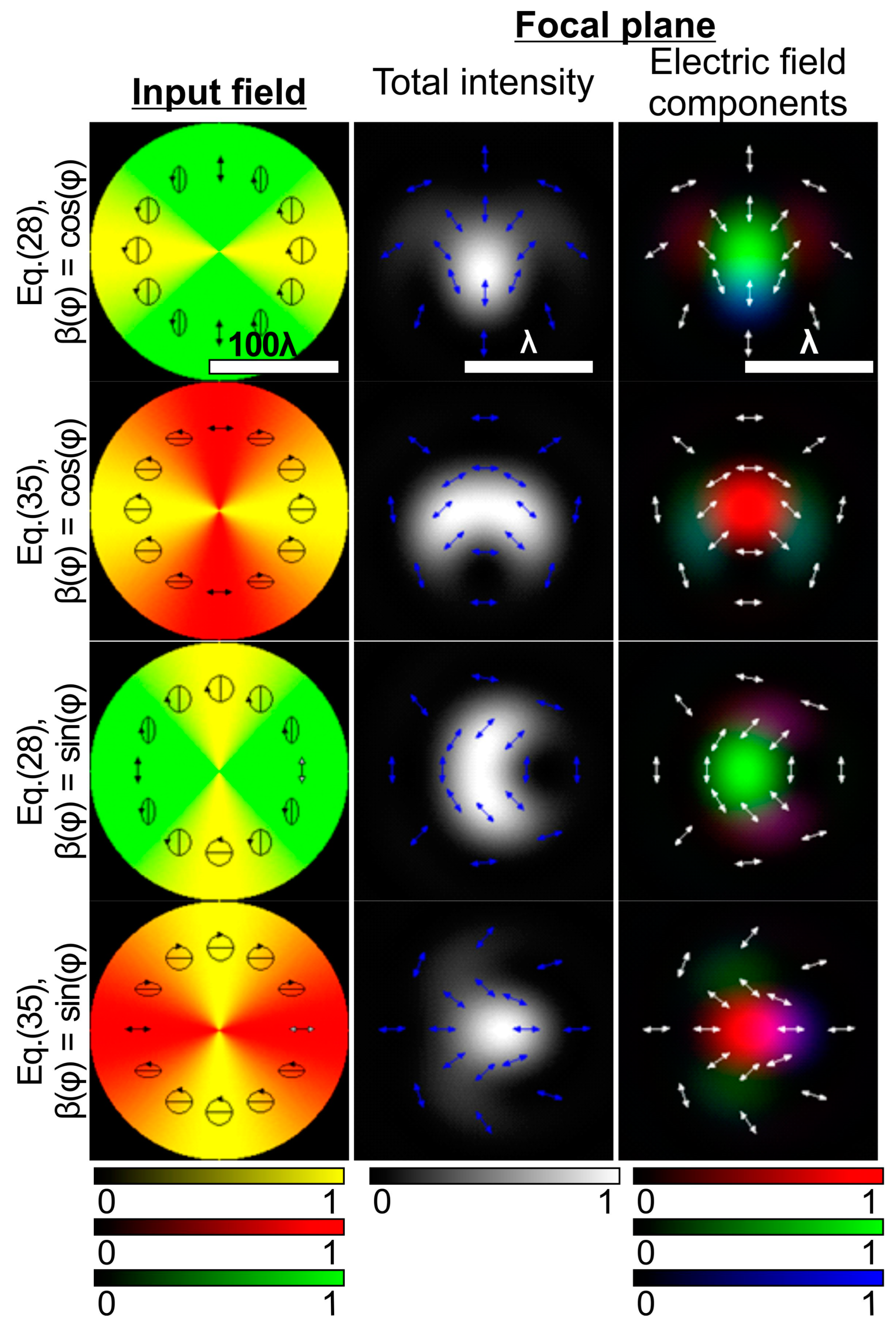
3.2. Variable Ratio of the Semi-Axes of the Polarization Ellipse

In this section, we consider a different situation, namely, we fix the inclination angle of the ellipse and introduce variations in the semi-axis ratio. Notably, at an angle of inclination equal to 0 or 90 degrees, the semi-axes ratio is equal to the amplitudes A_x and A_y ratio.

For definiteness, let us assume that the major semi-axis is located vertically (the angle of inclination is 90 degrees), and we denote its value by A. In this case, the minor semi-axis varies depending on the position in accordance with some function β(θ, φ) and is equal to Aβ(θ, φ). Let us assume that β(θ, φ) is a real function with $\left|\beta (\mathsf{\theta },\mathsf{\phi })\right|\le 1$. In this case, the components of the electric field are expressed by the formulas:

$$\begin{array}{l}{E}_{0x}=A\beta (\mathsf{\theta },\mathsf{\phi }),\\ E_{0y}=iA.\end{array}$$

(26)

For convenience, we regard dependence just on the polar angle: β(θ, φ) = β(φ). Next, we consider specific examples of the dependence β(φ).

3.2.1. Simple Trigonometric Dependence on the Polar Angle

Here, we consider a simple trigonometric dependence on the angle:

$$\beta (\mathsf{\phi })=\cos (\mathsf{\phi }).$$

(27)

Then, the input field will take the form:

$$\begin{array}{l}{E}_{0x}=A\cos \mathsf{\phi },\\ E_{0y}=iA.\end{array}$$

(28)

Similar to the analytical calculations from Section 3.1.1, we obtain:

$$\left[\begin{array}{l}{E}_x\\ E_y\\ E_z\end{array}\right]=-\frac{if}{\lambda }A{\displaystyle \underset{0}{\overset{\Theta }{\int }}T(\mathsf{\theta })F(\mathsf{\theta })\sin \mathsf{\theta }\left[\begin{array}{l}{S}_{1,0}-(1-\cos \mathsf{\theta })\left[S_{3,0}+i{S}_{1,1}\right]\\ i{S}_{0,0}-(1-\cos \mathsf{\theta })\left[S_{2,1}+i{S}_{0,2}\right]\\ -\sin \mathsf{\theta }\left[S_{2,0}+i{S}_{0,1}\right]\end{array}\right]d\mathsf{\theta }}$$

(29)

$$\left[\begin{array}{l}{H}_x\\ H_y\\ H_z\end{array}\right]=-\frac{if}{\lambda }A{\displaystyle \underset{0}{\overset{\Theta }{\int }}T(\mathsf{\theta })F(\mathsf{\theta })\sin \mathsf{\theta }\left[\begin{array}{l}-i{S}_{0,0}-(1-\cos \mathsf{\theta })\left[S_{2,1}-i{S}_{2,0}\right]\\ S_{1,0}-(1-\cos \mathsf{\theta })\left[S_{1,2}-i{S}_{1,1}\right]\\ -\sin \mathsf{\theta }\left[S_{1,1}-i{S}_{1,0}\right]\end{array}\right]d\mathsf{\theta }}$$

(30)

The S_p,_q expressions are given in Equation (14).

After substituting expressions (14) into Equations (29) and (30) for a narrow annular aperture, we obtain approximate analytical expressions:

$$\begin{array}{l}{E}_x=\frac{kf}{2}A\cdot \Delta \cdot T({\mathsf{\theta }}_0)F({\mathsf{\theta }}_0)\sin {\mathsf{\theta }}_0\times \\ \times \left\{0.5\left(1+3\cos {\mathsf{\theta }}_0\right)J_1(a)\cos \upsilon +\left(1-\cos {\mathsf{\theta }}_0\right)J_2(a)\sin 2\upsilon +0.5\left(1-\cos {\mathsf{\theta }}_0\right)J_3(a)\cos 3\upsilon \right\},\\ E_y=\frac{kf}{2}A\cdot \Delta \cdot T({\mathsf{\theta }}_0)F({\mathsf{\theta }}_0)\sin {\mathsf{\theta }}_0\times \\ \times \left\{\left(1+\cos {\mathsf{\theta }}_0\right)J_0(a)-\left(1-\cos {\mathsf{\theta }}_0\right)J_2(a)\cos 2\upsilon +0.5\left(1-\cos {\mathsf{\theta }}_0\right)\left[J_3(a)\sin 3\upsilon -J_1(a)\sin \upsilon \right]\right\},\\ E_z=-\frac{ikf}{2}A\cdot \Delta \cdot T({\mathsf{\theta }}_0)F({\mathsf{\theta }}_0){\sin }^2{\mathsf{\theta }}_0\left[-J_0(a)+2J_1(a)\sin \upsilon +J_2(a)\cos 2\upsilon \right].\end{array}$$

(31)

$$\begin{array}{l}{H}_x=\frac{kf}{2}A\cdot \Delta \cdot T({\mathsf{\theta }}_0)F({\mathsf{\theta }}_0)\sin {\mathsf{\theta }}_0\times \\ \times \left\{-\left(1+\cos {\mathsf{\theta }}_0\right)J_0(a)-\left(1-\cos {\mathsf{\theta }}_0\right)J_2(a)\cos 2\upsilon -0.5\left(1-\cos {\mathsf{\theta }}_0\right)\left[J_1(a)\sin \upsilon -J_3(a)\sin 3\upsilon \right]\right\},\\ H_y=\frac{kf}{2}A\cdot \Delta \cdot T({\mathsf{\theta }}_0)F({\mathsf{\theta }}_0)\sin {\mathsf{\theta }}_0\times \\ \times \left\{0.5\left(3+\cos {\mathsf{\theta }}_0\right)J_1(a)\cos \upsilon -\left(1-\cos {\mathsf{\theta }}_0\right)J_2(a)\sin 2\upsilon -0.5\left(1-\cos {\mathsf{\theta }}_0\right)J_3(a)\cos 3\upsilon \right\},\\ H_z=-\frac{ikf}{2}A\cdot \Delta \cdot T({\mathsf{\theta }}_0)F({\mathsf{\theta }}_0){\sin }^2{\mathsf{\theta }}_0\left[-2J_1(a)\cos \upsilon +J_2(a)\sin 2\upsilon \right].\end{array}$$

(32)

As follows from Equations (31) and (32), the transverse components of the electric and magnetic field are real, while the longitudinal components are purely imaginary.

The total intensity is

$$\begin{array}{l}{I}_{tot}={\left(\frac{kf}{2}A\cdot \Delta \cdot T({\mathsf{\theta }}_0)F({\mathsf{\theta }}_0)\sin {\mathsf{\theta }}_0\right)}^2\times \\ \times \left\{\begin{array}{l}{J}_0^2(a)\left(2+2\cos {\mathsf{\theta }}_0\right)+J_1^2(a)\left[4{\sin }^2{\mathsf{\theta }}_0{\sin }^2\upsilon +0.25{\left(1-\cos {\mathsf{\theta }}_0\right)}^2+\left(2\cos {\mathsf{\theta }}_0+2{\cos }^2{\mathsf{\theta }}_0\right){\cos }^2\upsilon \right]+\\ +J_2^2(a)\left[{\sin }^2{\mathsf{\theta }}_0{\cos }^{2}2\upsilon +{\left(1-\cos {\mathsf{\theta }}_0\right)}^2\right]+J_3^2(a)\cdot 0.25{\left(1-\cos {\mathsf{\theta }}_0\right)}^2-J_0(a)J_1(a)\cdot 5{\sin }^2{\mathsf{\theta }}_0\sin \upsilon -\\ -J_0(a)J_2(a)\cdot 4{\sin }^2{\mathsf{\theta }}_0\cos 2\upsilon +J_0(a)J_3(a)\cdot {\sin }^2{\mathsf{\theta }}_0\sin 3\upsilon +\\ +J_1(a)J_2(a)\left[4{\sin }^2{\mathsf{\theta }}_0\sin \upsilon \cos 2\upsilon +2{\sin }^2{\mathsf{\theta }}_0\cos \upsilon \sin 2\upsilon -{\left(1-\cos {\mathsf{\theta }}_0\right)}^2\sin \upsilon \right]+\\ +J_1(a)J_3(a)\left[{\sin }^2{\mathsf{\theta }}_0\cos \upsilon \cos 3\upsilon -0.5{\left(1-\cos {\mathsf{\theta }}_0\right)}^2\cos 2\upsilon \right]-J_2(a)J_3(a)\cdot {\left(1-\cos {\mathsf{\theta }}_0\right)}^2\sin \upsilon \end{array}\right\}\end{array}.$$

(33)

It can be seen that this expression is much more complex compared with Equation (18).

Since the smallest dependence of the polar angle is cos(υ)/sin(υ), the rotational symmetry should not be observed, but Equation (33) is the same for the angles υ = 90° ± υ1, so there will be symmetry about the vertical axis (it is seen in the first line of Figure 8).

About the Poynting vector, even before calculations, we can say that its longitudinal component is real, and the transverse components are purely imaginary. The expression for the longitudinal component is as follows:

$$\begin{array}{l}{S}_z=A^2{\left(\frac{kf}{2}\Delta \cdot T({\mathsf{\theta }}_0)F({\mathsf{\theta }}_0)\sin {\mathsf{\theta }}_0\right)}^2\times \\ \times \left\{\begin{array}{l}{J}_0^2(a){\left(1+\cos {\mathsf{\theta }}_0\right)}^2+J_1^2(a)\cdot 0.25\left[\left(1+3\cos {\mathsf{\theta }}_0\right)\left(3+\cos {\mathsf{\theta }}_0\right){\cos }^2\upsilon -{\left(1-\cos {\mathsf{\theta }}_0\right)}^2{\sin }^2\upsilon \right]-\\ -J_2^2(a){\left(1-\cos {\mathsf{\theta }}_0\right)}^2-J_3^2(a)\cdot 0.25{\left(1-\cos {\mathsf{\theta }}_0\right)}^2+J_1(a)J_2(a){\left(1-\cos {\mathsf{\theta }}_0\right)}^2\sin \upsilon +\\ +J_1(a)J_3(a)\cdot 0.5{\left(1-\cos {\mathsf{\theta }}_0\right)}^2\cos 2\upsilon +J_2(a)J_3(a){\left(1-\cos {\mathsf{\theta }}_0\right)}^2\sin \upsilon \end{array}\right\}\end{array}$$

(34)

It can be seen that expression (34) is simpler than Equation (33) for the intensity.

Obviously, similar results can be obtained if we assume that the axis of the ellipse is horizontal, then the input field is presented in the following form:

$$\begin{array}{l}{E}_{0x}=A,\\ E_{0y}=iA\cos \mathsf{\phi }.\end{array}$$

(35)

In addition, one can change the dependency to a function β(φ) = sin(φ).

Figure 8 shows the calculations of the formation of fields with inhomogeneous elliptical polarization at $\beta (\mathsf{\phi })=\left\{\begin{array}{c}\cos (\mathsf{\phi })\\ \sin (\mathsf{\phi })\end{array}\right\}$ for various positions of the polarization axis corresponding to Equations (28) and (35).

Several remarks can be made on the results in Figure 8. It can be seen that the rotation of the polarization ellipse or the change of the trigonometric function leads to a qualitative change in the intensity pattern: comparing rows 1 and 2, 3 and 4, 1 and 3, or 2 and 4. However, if we do both transformations, there will only be a rotation of the distribution of all components (not just the total intensity) by 90 degrees: comparing rows 1 and 4 or 2 and 3. It is also clearly seen that in the focal plane at all local points, the polarization is linear. This happens because both transverse components are either real (Equation (28), and for β(φ) = cos(φ) Equation (31)) or purely imaginary (Equation (35)) (in fact, they are also real with the same additional phase). In both cases, linear polarization is obtained. Note that this situation takes place not only for a narrow annular aperture since the transverse components do not change during integration.

3.2.2. Multiple and Power Trigonometric Dependence on the Polar Angle

An obvious generalization of function in Equation (27), which specifies variations in the ratio of the semi-axes of the polarization ellipse, is a multiple trigonometric dependence on the polar angle:

$$\beta (\mathsf{\phi })=\left\{\begin{array}{c}\cos (m\mathsf{\phi })\\ \sin (m\mathsf{\phi })\end{array}\right\},$$

(36)

as well as the power dependence:

$$\beta (\mathsf{\phi })=\left\{\begin{array}{c}{\cos }^p(\mathsf{\phi })\\ {\sin }^p(\mathsf{\phi })\end{array}\right\}.$$

(37)

Note that for positive integer p, Equation (37) can be reduced to a superposition of functions in the form of Equation (36).

An analytical representation in these cases (for integer m and positive integer p) can also be obtained, but it will be even more cumbersome, so we present only the results of numerical simulation.

Figure 9 shows calculations of the formation of fields with non-uniform elliptical polarization at $\beta (\mathsf{\phi })=\left\{\begin{array}{c}\cos (m\mathsf{\phi })\\ \sin (m\mathsf{\phi })\end{array}\right\}$, and Figure 10 shows the results for $\beta (\mathsf{\phi })=\left\{\begin{array}{c}{\cos }^p(\mathsf{\phi })\\ {\sin }^p(\mathsf{\phi })\end{array}\right\}$.

As can be seen from Figure 9, if m is odd, then the polarization is linear in all local points of the focal plane. This can be explained by the fact that for both types of input field (Equation (28) or Equation (35)) the transverse components are of the same type when m is odd: both real (for Equation (28)), or both are purely imaginary (for Equation (35)).

An example in Figure 8 is a special case (m = 1). This follows from Equation (3), formulas for converting the product of trigonometric functions into a sum, and Equation (22).

One can also be sure that at Equation (35) and β(φ) = sin(2φ) the y-component is equal to zero in those regions where sin(2υ) = 0, i.e., along the vertical and horizontal lines (this is clearly seen in the first line in Figure 9).

The results in Figure 10 are similar to those shown in Figure 9. It can be seen that if p is odd, the polarization is linear in all local points of the focal plane. The proof is based on a reduction to the previous case based on degree reduction: sin^p(φ) for odd p is expressed through sin(q_nφ) where all q_n are odd, and for even p, it is expressed through cos(q_nφ) where all q_n are even. Similarly, cos^p(φ) is expressed in terms of cos(q_nφ) where all q_n have the same parity as p. Therefore, the power dependence provides a locally linear polarization in similar situations as for the multiple ones.

Figure 11 shows the results of calculating the longitudinal component of the Poynting vector by Equation (7) for the functions β(φ) = cos(mφ) at different values of m (for the Equation (35) variant).

Note that for odd integer values of m, there is no imaginary part (in this case, the situation is similar to that considered in Section 3.1), but the regions with negative values are not observed in the real part. For integer even m, the imaginary part contains the symmetric areas with positive and negative values ( in the 2nd column in Figure 11), so the total value is zero. For fractional m, the situation is different (in the 3rd column in Figure 11) in terms of symmetry breaking.

Figure 11 also shows the corresponding pictures of the real parts of the transverse components of the Poynting vector. As can be seen, at m = 1, the real parts of the transverse components are missing, and for m = 2 and m = 1.5, the flow is sufficiently complex.

4. Discussion and Conclusions

Summing up, in this work, we presented the results of the shaping of focused structured laser beams with controlled locally inhomogeneous parameters of elliptical polarization. It is possible to control the ellipticity of the formed polarization ellipse at each point of the focused light field, the orientation, and the rotation direction of the polarization vector. For example, we can create a focused annular light field with radial polarization in the inner part of the formed ring and elliptical polarization with a rotated orientation in the outer part of the ring. It is also possible to create a light field with a continuous change in the ellipticity and orientation of the polarization ellipse across the focused light ring.

To implement such full control of the polarization parameters, we used high-NA focusing, structured laser beams with a predetermined structure of the transverse components of the electromagnetic field. However, when the NA is reduced, some of the properties of the generated beams will remain the same. In particular, the distribution of transverse components that determine the polarization state of the formed beam will be preserved (up to scale). As NA decreases, the contribution of the longitudinal component will also diminish. The area and magnitude of the reverse energy flow will also decrease, as indicated earlier [78].

Currently, there are various methods for shaping such structured laser beams—the use of subwavelength gratings, patterned micro-retarder arrays, polarization sector plates, or spatial light modulators [14,23,31,32,33,35,40]. In our opinion, the use of single or two spatial light modulators for the implementation of an interferometric approach for the summation of two orthogonally polarized laser modes is the most convenient method [31,32,33]. In this case, we can dynamically change the distributions of each component of the formed modes and fine-tune the parameters of the inhomogeneous elliptical polarization distribution of the generated fields for laser material processing and laser manipulation applications. Previously, such methods were used to generate different types of vector beams.

Unlike other studies devoted to the formation of vector laser beams with hybrid polarization states, we investigated the formation of vector laser beams by focusing on such beams. The generation of focused vector laser beams is of crucial importance in modern advanced optical tweezers and laser material processing. Controlling not only the amplitude and phase but also the polarization distribution of the shaped optical tweezers can be used to control the density of SAM and OAM of the light fields, as well as to implement spin-orbit conversion and generate light fields with reverse energy flow. The formation of sharply focused laser beams with a non-uniform distribution of elliptical polarization is one of the possible ways to control the morphology of LIPSSs, which mainly determines the functional properties of the treated materials and the spectrum of their potential applications [20,47,48]. Thus, the development of simple and effective methods for generating laser beams with the possibility to control their complex structure is the key to further development of laser processing technology. The ability to manipulate complex polarization distributions in a focused structured laser beam will provide feedback that can control the nanomorphology of the laser-treated surface, such as enhancing or suppressing the formation of LIPSSs at a given point on the surface during laser processing.

References

1. Forbes, A. Structured Light from Lasers. Laser Photon. Rev. 2019, 13, 1900140. [Google Scholar] [CrossRef]
2. Angelsky, O.V.; Bekshaev, A.Y.; Hanson, S.G.; Zenkova, C.Y.; Mokhun, I.I.; Jun, Z. Structured Light: Ideas and Concepts. Front. Phys. 2020, 8, 114. [Google Scholar] [CrossRef]
3. Forbes, A.; de Oliveira, M.; Dennis, M.R. Structured Light. Nat. Photonics 2021, 15, 253–262. [Google Scholar] [CrossRef]
4. Andrews, D.L. Structured Light and Its Applications: An Introduction to Phase Structured Beams and Nanoscale Optical Forces; Academic Press: Cambridge, MA, USA, 2011. [Google Scholar]
5. Padgett, M.J.; Bowman, R. Tweezers with a Twist. Nat. Photonics 2011, 5, 343–348. [Google Scholar] [CrossRef]
6. Litchinitser, N.M. Structured Light Meets Structured Matter. Science 2012, 337, 1054–1055. [Google Scholar] [CrossRef]
7. Du, J.; Wang, J. High-Dimensional Structured Light Coding/Decoding for Freespace Optical Communications Free of Obstructions. Opt. Lett. 2015, 40, 4827–4857. [Google Scholar] [CrossRef] [PubMed]
8. Rosales-Guzmán, C.; Ndagano, B.; Forbes, A. A Review of Complex Vector Light Fields and Their Applications. J. Opt. 2018, 20, 123001. [Google Scholar] [CrossRef]
9. Angelo, J.P.; Chen, S.-J.; Ochoa, M.; Sunar, U.; Gioux, S.; Intes, X. Review of Structured Light in Diffuse Optical Imaging. J. Biomed. Opt. 2018, 24, 071602. [Google Scholar] [CrossRef] [PubMed]
10. Khonina, S.N. Vortex Beams with High-Order Cylindrical Polarization: Features of Focal Distributions. Appl. Phys. B 2019, 125, 100. [Google Scholar] [CrossRef]
11. Flamm, D.; Grossmann, D.G.; Sailer, M.; Kaiser, M.; Zimmermann, F.; Chen, K.; Jenne, M.; Kleiner, J.; Hellstern, J.; Tillkorn, C.; et al. Structured Light for Ultrafast Laser Micro- and Nanoprocessing. Opt. Eng. 2021, 60, 025105. [Google Scholar] [CrossRef]
12. Yang, Y.; Ren, Y.X.; Chen, M.; Arita, Y.; Rosales-Guzmán, C. Optical Trapping with Structured Light: A Review. Adv. Photon. 2021, 3, 034001. [Google Scholar] [CrossRef]
13. Porfirev, A.P.; Kuchmizhak, A.A.; Gurbatov, S.O.; Juodkazis, S.; Khonina, S.N.; Kulchin, Y.N. Phase Singularities and Optical Vortices in Photonics. Phys. Usp. 2022, 65, 789–811. [Google Scholar] [CrossRef]
14. Khonina, S.N.; Porfirev, A.P. Harnessing of Inhomogeneously Polarized Hermite–Gaussian Vector Beams to Manage the 3D Spin Angular Momentum Density Distribution. Nanophotonics 2022, 11, 697–712. [Google Scholar] [CrossRef]
15. Porfirev, A.; Khonina, S.; Kuchmizhak, A. Light–Matter Interaction Empowered by Orbital Angular Momentum: Control of Matter at The Micro-And Nanoscale. Prog. Quantum Electron. 2023, 88, 100459. [Google Scholar] [CrossRef]
16. Prasciolu, M.; Tamburini, F.; Anzolin, G.; Mari, E.; Melli, M.; Carpentiero, A.; Barbieri, C.; Romanato, F. Fabrication of a Three-Dimensional Optical Vortices Phase Mask for Astronomy by Means of Electron-Beam Lithography. Microelectron Eng. 2009, 86, 1103–1106. [Google Scholar] [CrossRef]
17. Massari, M.; Ruffato, G.; Gintoli, M.; Ricci, F.; Romanato, F. Fabrication and Characterization of High-Quality Spiral Phase Plates for Optical Applications. Appl. Opt. 2015, 54, 4077–4083. [Google Scholar] [CrossRef]
18. Forbes, A.; Dudley, A.; McLaren, M. Creation and Detection of Optical Modes with Spatial Light Modulators. Adv. Opt. Photon. 2016, 8, 200–227. [Google Scholar] [CrossRef]
19. Yue, F.; Wen, D.; Xin, J. Vector Vortex Beam Generation with a Single Plasmonic Metasurface. ACS Photonics 2016, 3, 1558. [Google Scholar] [CrossRef]
20. Nivas, J.J.J.; Allahyari, E.; Cardano, F.; Rubano, A.; Fittipaldi, R.; Vecchione, A.; Paparo, D.; Marrucci, L.; Bruzzese, R.; Amoruso, S. Surface Structures with Unconventional Patterns and Shapes Generated by Femtosecond Structured Light Fields. Sci. Rep. 2018, 8, 13613. [Google Scholar] [CrossRef]
21. Khonina, S.N.; Porfirev, A.P.; Kazanskiy, N.L. Variable Transformation of Singular Cylindrical Vector Beams Using Anisotropic Crystals. Sci. Rep. 2020, 10, 5590. [Google Scholar] [CrossRef]
22. Wang, J.; Liang, Y. Generation and Detection of Structured Light: A Review. Front. Phys. 2021, 9, 688284. [Google Scholar] [CrossRef]
23. Khonina, S.N.; Degtyarev, S.A.; Ustinov, A.V.; Porfirev, A.P. Metalenses for the Generation of Vector Lissajous Beams with a Complex Poynting Vector Density. Opt. Express 2021, 29, 18651–18662. [Google Scholar] [CrossRef] [PubMed]
24. Ahmed, H.; Kim, H.; Zhang, Y.; Intaravanne, Y.; Jang, J.; Rho, J.; Chen, S.; Chen, X. Optical Metasurfaces for Generating and Manipulating Optical Vortex Beams. Nanophotonics 2022, 11, 941–956. [Google Scholar] [CrossRef]
25. Zheng, S.; Zhao, Z.; Zhang, W. Versatile Generation and Manipulation of Phase-Structured Light Beams Using On-Chip Subwavelength Holographic Surface Gratings. Nanophotonics 2023, 12, 55–70. [Google Scholar] [CrossRef]
26. Zhu, L.; Wang, J. Simultaneous Generation of Multiple Orbital Angular Momentum (OAM) Modes Using a Single Phase-Only Element. Opt Express 2015, 23, 26221–26233. [Google Scholar] [CrossRef]
27. Mingyang, S.; Junmin, L.; Yanliang, H.; Shuqing, C.; Ying, L. Optical Orbital Angular Momentum Demultiplexing and Channel Equalization by Using Equalizing Dammann Vortex Grating. Adv. Condens. Matter Phys. 2017, 2017, 6293910. [Google Scholar]
28. Khonina, S.N.; Karpeev, S.V.; Paranin, V.D. A Technique for Simultaneous Detection of Individual Vortex States of Laguerre–Gaussian Beams Transmitted through an Aqueous Suspension of Microparticles. Opt. Lasers Eng. 2018, 105, 68–74. [Google Scholar] [CrossRef]
29. Qiao, Z.; Wan, Z.Y.; Xie, G.Q.; Wang, J.; Qian, L.J.; Fan, D.Y. Multi-Vortex Laser Enabling Spatial and Temporal Encoding. PhotoniX 2020, 1, 13. [Google Scholar] [CrossRef]
30. Ni, J.; Huang, C.; Zhou, L.M.; Gu, M.; Song, Q.; Kivshar, Y.; Qiu, C.W. Multidimensional Phase Singularities in Nanophotonics. Science 2021, 374, eabj0039. [Google Scholar] [CrossRef]
31. Maurer, C.; Jesacher, A.; Fürhapter, S.; Bernet, S.; Ritsch-Marte, M. Tailoring of Arbitrary Optical Vector Beams. New J. Phys. 2007, 9, 78. [Google Scholar] [CrossRef]
32. Man, Z.; Min, C.; Zhang, Y.; Shen, Z.; Yuan, X.-C. Arbitrary Vector Beams with Selective Polarization States Patterned by Tailored Polarizing Films. Laser Phys. 2013, 23, 105001. [Google Scholar] [CrossRef]
33. Chen, S.; Zhou, X.; Liu, Y.; Ling, X.; Luo, H.; Wen, S. Generation of Arbitrary Cylindrical Vector Beams on the Higher Order Poincaré Sphere. Opt. Lett. 2014, 39, 5274–5276. [Google Scholar] [CrossRef] [PubMed]
34. Millione, G.; Nguyen, T.A.; Leach, J.; Nolan, D.A.; Alfano, R.R. Using the Nonseparability of Vector Beams to Encode Information for Optical Communication. Opt. Lett. 2015, 40, 4887–4890. [Google Scholar] [CrossRef] [PubMed]
35. Khonina, S.N.; Ustinov, A.V.; Fomchenkov, S.A.; Porfirev, A.P. Formation of Hybrid Higher-Order Cylindrical Vector Beams Using Binary Multi-Sector Phase Plates. Sci. Rep. 2018, 8, 14320. [Google Scholar] [CrossRef]
36. Wu, H.J.; Zhao, B.; Rosales-Guzmán, C.; Gao, W.; Shi, B.S.; Zhu, Z.H. Spatial-Polarization-Independent Parametric Up-Conversion of Vectorially Structured Light. Phys. Rev. Appl. 2020, 13, 064041. [Google Scholar] [CrossRef]
37. Huang, H.; Xie, G.; Yan, Y.; Ahmed, N.; Ren, Y.; Yue, Y.; Rogawski, D.; Willner, M.J.; Erkmen, B.I.; Birnbaum, K.M.; et al. 100 Tbit/s Free-Space Data Link Enabled by Three-Dimensional Multiplexing of Orbital Angular Momentum, Polarization, And Wavelength. Opt. Lett. 2014, 39, 197–200. [Google Scholar] [CrossRef]
38. Mitchell, K.J.; Turtaev, S.; Padgett, M.J.; Cižmár, T.; Phillips, D.B. High-Speed Spatial Control of the Intensity, Phase and Polarisation of Vector Beams Using a Digital Micro-Mirror Device. Opt Express 2016, 24, 29269–29282. [Google Scholar] [CrossRef]
39. Chen, Y.; Lin, Z.; Villers, S.B.D.; Rusch, L.A.; Shi, W. WDM-Compatible Polarization-Diverse OAM Generator and Multiplexer in Silicon Photonics. IEEE J. Sel. Top. Quantum Electron. 2020, 26, 6100107. [Google Scholar] [CrossRef]
40. Khonina, S.N.; Karpeev, S.V.; Porfirev, A.P. Sector Sandwich Structure: An Easy-to-Manufacture Way Towards Complex Vector Beam Generation. Opt. Express 2020, 28, 27628–27643. [Google Scholar] [CrossRef]
41. Dorrah, A.H.; Rubin, N.A.; Tamagnone, M.; Zaidi, A.; Capasso, F. Structuring Total Angular Momentum of Light Along the Propagation Direction with Polarization-Controlled Meta-Optics. Nat. Commun. 2021, 12, 6249. [Google Scholar] [CrossRef]
42. Khonina, S.N.; Kazanskiy, N.L.; Butt, M.A.; Karpeev, S.V. Optical Multiplexing Techniques and Their Marriage for On-Chip and Optical Fiber Communication: A Review. Opto-Electronic Adv. 2022, 5, 210127. [Google Scholar]
43. He, C.; Shen, Y.; Forbes, A. Towards Higher-Dimensional Structured Light. Light Sci. Appl. 2022, 11, 205. [Google Scholar] [CrossRef]
44. Dorn, R.; Quabis, S.; Leuchs, G. Sharper Focus for a Radially Polarized Light Beam. Phys. Rev. Lett. 2003, 91, 233901. [Google Scholar] [CrossRef]
45. Wang, H.; Shi, L.; Lukyanchuk, D.; Sheppard, C.; Chong, C.T. Creation of a Needle of Longitudinally Polarized Light in Vacuum Using Binary Optics. Nat. Photonics 2008, 2, 501–505. [Google Scholar] [CrossRef]
46. Jin, Y.; Allegre, O.J.; Perrie, W.; Abrams, K.; Ouyang, J.; Fearon, E.; Edwardson, S.P.; Dearden, G. Dynamic Modulation of Spatially Structured Polarization Fields for Real-Time Control of Ultrafast Laser-Material Interactions. Opt. Express 2013, 21, 25333–25343. [Google Scholar] [CrossRef]
47. Anoop, K.K.; Rubano, A.; Fittipaldi, R.; Wang, X.; Paparo, D.; Vecchione, A.; Marrucci, L.; Bruzzese, R.; Amoruso, S. Femtosecond Laser Surface Structuring of Silicon Using Optical Vortex Beams Generated by a Q-Plate. Appl. Phys. Lett. 2014, 104, 241604. [Google Scholar] [CrossRef]
48. Nivas, J.J.J.; Allahyari, E.; Amoruso, S. Direct Femtosecond Laser Surface Structuring with Complex Light Beams Generated by Q-Plates. Adv. Opt. Technol. 2020, 9, 53. [Google Scholar] [CrossRef]
49. Porfirev, A.; Khonina, S.; Ivliev, N.; Meshalkin, A.; Achimova, E.; Forbes, A. Writing and Reading with the Longitudinal Component of Light Using Carbazole-Containing Azopolymer Thin Films. Sci. Rep. 2022, 12, 3477. [Google Scholar] [CrossRef]
50. Porfirev, A.P.; Khonina, S.N.; Ivliev, N.A.; Fomchenkov, S.A.; Porfirev, D.P.; Karpeev, S.V. Polarization-Sensitive Patterning of Azopolymer Thin Films Using Multiple Structured Laser Beams. Sensors 2023, 23, 112. [Google Scholar] [CrossRef]
51. Moreno, I.; Davis, J.A.; Ruiz, I.; Cottrell, D.M. Decomposition of Radially and Azimuthally Polarized Beams Using a Circular-Polarization and Vortex-Sensing Diffraction Grating. Opt. Express 2010, 18, 7173–7183. [Google Scholar] [CrossRef]
52. Zhou, Z.-H.; Guo, Y.-K.; Zhu, L.-Q. Tight Focusing of Axially Symmetric Polarized Vortex Beams. Chin. Phys. B 2014, 23, 044201. [Google Scholar] [CrossRef]
53. Porfirev, A.P.; Ustinov, A.V.; Khonina, S.N. Polarization Conversion When Focusing Cylindrically Polarized Vortex Beams. Sci. Rep. 2016, 6, 6. [Google Scholar] [CrossRef] [PubMed]
54. Khonina, S.N.; Porfirev, A.P.; Karpeev, S.V. Recognition of Polarization and Phase States of Light Based on the Interaction of Nonuniformly Polarized Laser Beams with Singular Phase Structures. Opt. Express 2019, 27, 18484–18492. [Google Scholar] [CrossRef]
55. Wang, X.-L.; Li, Y.; Chen, J.; Guo, C.-S.; Ding, J.; Wang, H.-T. A New Type of Vector Fields with Hybrid States of Polarization. Opt. Express 2010, 18, 10786–10795. [Google Scholar] [CrossRef] [PubMed]
56. Pu, J.; Zhang, Z. Tight Focusing of Spirally Polarized Vortex Beams. Opt. Laser Technol. 2010, 42, 186–191. [Google Scholar] [CrossRef]
57. Man, Z.; Min, C.; Zhu, S.; Yuan, X.-C. Tight Focusing of Quasi-Cylindrically Polarized Beams. J. Opt. Soc. Am. A 2014, 31, 373–378. [Google Scholar] [CrossRef]
58. Pan, Y.; Gao, X.-Z.; Zhang, G.-L.; Li, Y.; Tu, C.; Wang, H.-T. Spin Angular Momentum Density and Transverse Energy Flow of Tightly Focused Kaleidoscope-Structured Vector Optical Fields. APL Photonics 2019, 4, 096102. [Google Scholar] [CrossRef]
59. Zhao, Y.; Edgar, J.S.; Jeffries, G.D.M.; McGloin, D.; Chiu, D.T. Spin-to-Orbital Angular Momentum Conversion in a Strongly Focused Optical Beam. Phys. Rev. Lett. 2007, 99, 073901. [Google Scholar] [CrossRef]
60. Zhu, J.; Chen, Y.; Zhang, Y.; Cai, X.; Yu, S. Spin and Orbital Angular Momentum and Their Conversion in Cylindrical Vector Vortices. Opt. Lett. 2014, 39, 4435–4438. [Google Scholar] [CrossRef]
61. Bliokh, K.Y.; Rodriguez-Fortuno, F.; Nori, F.; Zayats, A.V. Spin-Orbit Interactions of Light. Nat. Photonics 2015, 9, 796–808. [Google Scholar] [CrossRef]
62. Devlin, R.C.; Ambrosio, A.; Rubin, N.A.; Mueller, J.P.B.; Capasso, F. Arbitrary Spin-to–Orbital Angular Momentum Conversion of Light. Science 2017, 358, 896–901. [Google Scholar] [CrossRef] [PubMed]
63. Khonina, S.N.; Golub, I. Vectorial Spin Hall Effect of Light Upon Tight Focusing. Opt. Lett. 2022, 47, 2166. [Google Scholar] [CrossRef] [PubMed]
64. Cheng, J.; Zhang, Z.; Mei, W.; Cao, Y.; Ling, X.; Chen, Y. Symmetry-Breaking Enabled Topological Phase Transitions in Spin-Orbit Optics. Opt. Express 2023, 31, 23621. [Google Scholar] [CrossRef] [PubMed]
65. Freund, I.; Soskin, M.S.; Mokhun, A.I. Elliptic Critical Points in Paraxial Optical Fields. Opt. Commun. 2002, 208, 223–253. [Google Scholar] [CrossRef]
66. Vyas, S.; Kozawa, Y.; Sato, S. Polarization Singularities in Superposition of Vector Beams. Opt. Express 2013, 21, 8972–8986. [Google Scholar] [CrossRef]
67. Kumar, V.; Philip, G.M.; Viswanathan, N.K. Formation and Morphological Transformation of Polarization Singularities: Hunting the Monstar. J. Opt. 2013, 15, 044027. [Google Scholar] [CrossRef]
68. Senthilkumaran, R.P.; Pal, S.K. Phase Singularities to Polarization Singularities. Int. J. Opt. 2020, 2020, 2812803. [Google Scholar]
69. Kotlyar, V.V.; Stafeev, S.S.; Nalimov, A.G. Sharp Focusing of a Hybrid Vector Beam with a Polarization Singularity. Photonics 2021, 8, 227. [Google Scholar] [CrossRef]
70. Bonse, J.; Höhm, S.; Kirner, S.V.; Rosenfeld, A.; Krüger, J. Laser-Induced Periodic Surface Structures—A Scientific Evergreen. IEEE J. Sel. Top. Quantum Electron. 2016, 23, 9000615. [Google Scholar] [CrossRef]
71. Richards, B.; Wolf, E. Electromagnetic Diffraction in Optical Sysems. II. Structure of the Aplanatic System. Proc. R. Soc. Lond. 1959, 253, 358. [Google Scholar]
72. Pereira, S.F.; van de Nes, A.S. Superresolution by Means of Polarisation, Phase and Amplitude Pupil Masks. Opt. Commun. 2004, 234, 119. [Google Scholar] [CrossRef]
73. Khonina, S.N.; Golub, I. Engineering the Smallest 3D Symmetrical Bright and Dark Focal Spots. J. Opt. Soc. Am. A 2013, 30, 2029–2033. [Google Scholar] [CrossRef] [PubMed]
74. Bliokh, K.Y.; Bekshaev, A.Y.; Nori, F. Extraordinary Momentum and Spin in Evanescent Waves. Nat. Commun. 2014, 5, 3300. [Google Scholar] [CrossRef]
75. Xu, X.; Nieto-Vesperinas, M. Azimuthal Imaginary Poynting Momentum Density. Phys. Rev. Lett. 2019, 123, 233902. [Google Scholar] [CrossRef] [PubMed]
76. Khonina, S.N.; Porfirev, A.P.; Ustinov, A.V.; Kirilenko, M.S.; Kazanskiy, N.L. Tailoring of Inverse Energy Flow Profiles with Vector Lissajous Beams. Photonics 2022, 9, 121. [Google Scholar] [CrossRef]
77. Sheppard, C.J.R.; Choudhury, A. Annular Pupils, Radial Polarization, and Superresolution. Appl. Opt. 2004, 43, 4322–4327. [Google Scholar] [CrossRef]
78. Khonina, S.N.; Ustinov, A.V. Increased Reverse Energy Flux Area When Focusing a Linearly Polarized Annular Beam with Binary Plates. Opt. Lett. 2019, 44, 2008–2011. [Google Scholar] [CrossRef]
79. Man, Z.; Bai, Z.; Zhang, S.; Li, X.; Li, J.; Ge, X.; Zhang, Y.; Fu, S. Redistributing the energy flow of a tightly focused radially polarized optical field by designing phase masks. Opt. Express 2018, 26, 23935–23944. [Google Scholar] [CrossRef]
80. Man, Z.; Li, X.; Zhang, S.; Bai, Z.; Lyu, Y.; Li, J.; Ge, X.; Sun, Y.; Fu, S. Manipulation of the transverse energy flow of azimuthally polarized beam in tight focusing system. Opt. Commun. 2019, 431, 174–180. [Google Scholar] [CrossRef]
81. Kotlyar, V.V.; Kovalev, A.A.; Nalimov, A.G. Energy density and energy flux in the focus of an optical vortex: Reverse flux of light energy. Opt. Lett. 2018, 43, 2921. [Google Scholar] [CrossRef]
Figure 1. The polarization ellipse.
Photonics 10 01112 g001
Figure 2. Vector Debye theory of focusing an optical beam through a focusing system with a focal length f and maximum azimuthal angle Θ.
Photonics 10 01112 g002
Figure 3. Formation of fields with non-uniform elliptical polarization with α(φ) = φ: field type at the input (a,c) and in the focal plane (b,d) for Ax = Ay (a,b) and for Ax = 2Ay (c,d).
Photonics 10 01112 g003
Figure 4. Formation of fields with non-uniform elliptical polarization at α(φ) = 2φ. The arrows show local polarization directions.
Photonics 10 01112 g004
Figure 5. Formation of fields with non-uniform elliptical polarization at α(φ) = 3φ. The arrows show local polarization directions.
Photonics 10 01112 g005
Figure 6. Formation of fields with non-uniform elliptical polarization at α(φ) = 1.5φ. The arrows show local polarization directions.
Photonics 10 01112 g006
Figure 7. Distribution of the longitudinal component S z (two upper lines: blue color corresponds to positive values, turquoise color is for negative values) and square of the real parts of the transverse components Re S x 2 + Re S y 2 (bottom line: red color corresponds to x-component, green color corresponds to y-component, the direction of the transverse energy flow is shown by the black arrows) of the Poynting vector for various α(φ).
Photonics 10 01112 g007
Figure 8. Formation of fields with non-uniform elliptical polarization with a simple trigonometric dependence β(φ). The arrows show local polarization directions.
Photonics 10 01112 g008
Figure 9. Formation of fields with non-uniform elliptical polarization with a multiple trigonometric dependence β(φ). The arrows show local polarization directions.
Photonics 10 01112 g009
Figure 10. Formation of fields with non-uniform elliptical polarization with a power trigonometric dependence β(φ). The arrows show local polarization directions.
Photonics 10 01112 g010
Figure 11. Distribution of the longitudinal component S z (two upper lines) and square of the real parts of the transverse components Re S x 2 + Re S y 2 (the bottom line) of the Poynting vector for various β(φ). The direction of the transverse energy flow is shown by the black arrows.
Photonics 10 01112 g011
Disclaimer/Publisher’s Note: The statements, opinions and data contained in all publications are solely those of the individual author(s) and contributor(s) and not of MDPI and/or the editor(s). MDPI and/or the editor(s) disclaim responsibility for any injury to people or property resulting from any ideas, methods, instructions or products referred to in the content.