Article

Positioning of a Photovoltaic Device on a Real Two-Dimensional Plane in Optical Wireless Power Transmission by Means of Infrared Differential Absorption Imaging

Laboratory for Future Interdisciplinary Research of Science and Technology (FIRST), Institute of Innovative Research (IIR), Tokyo Institute of Technology, R2-39, 4259 Nagatsuta, Midori-ku, Yokohama 226-8503, Japan
*
Author to whom correspondence should be addressed.
Photonics 2023, 10(10), 1111; https://doi.org/10.3390/photonics10101111
Submission received: 16 July 2023 / Revised: 25 August 2023 / Accepted: 12 September 2023 / Published: 30 September 2023

Abstract

:
In optical wireless power transmission (OWPT), detection and positioning of the photovoltaic device (PV) in real space is essential before power transmission. One of the candidates for the robust detection of PVs is differential absorption imaging, which has been proposed by the authors. In this method, raw images are captured using absorbable ( λ O N ) and non-absorbable ( λ O F F ) wavelengths of the PV. Then, the PV is detected from the differential image of these. In this report, the positioning of a PV on a real two-dimensional plane was investigated by means of this differential imaging. Primarily, stereo imagery was utilized for positioning. Non-stereo positioning was also investigated, in which the azimuth angle (direction) was estimated from the position of the PV in the differential image, and ranging was performed using its apparent size. There are diffuse and non-diffuse (specular) options for the λ O F F reflection of the rear surface of the PV. Positioning accuracy was measured with regard to this characteristic as well as the attitude angle. Especially for a PV with specular characteristics, even though its positioning accuracy was affected by its attitude angle, the accuracy could be improved by increasing the irradiation light power. On the other hand, direction determination was stable for a wide angular range of attitudes.

1. Introduction

In the future, many power transmission systems to individual equipment are expected to become wireless [1], and optical wireless power transmission (OWPT) will play an important role [2,3,4]. Since it features light beams, it has an advantage of long-distance power transmission to photovoltaic devices (PVs) [5,6,7,8]. To increase the power generation efficiency in the target (PV), precise beam alignment and shaping depending on the target’s position is necessary [9,10], and the PV’s position and attitude needs to be determined from the light source before power transmission. Therefore, detecting the solar cells’ position and attitude is essential for any operational OWPT system. While there would be some navigation systems that might be available in an actual OWPT operation scene, it is uncertain if such a system can accommodate the requirements of an OWPT system. To build an OWPT system on a firm building block, a study of the primary positioning method intrinsic to the OWPT is necessary. Then, an external navigation system is used as a supplement. In former research, PV detection was studied by means of image processing of its outline or specific markers. It was reported that detection became unstable in the case of varying background illumination due to weather or time. Background conditions need to be taken into account in PV detection. These can vary with time, and targets can be lost by simple image processing under such varying illumination. The shapes and colors of some objects can be mistaken for real PVs. One of the candidates for robust PV detection is the differential absorption technique. It is used in many technical areas [11,12,13], and this has been applied to OWPT by the authors [14,15]. In this method, two independent images are captured with absorbable ( λ O N ) and non-absorbable ( λ O F F ) wavelengths of the PV. Then, a final image including the PV is generated by the differential image of these two images. Assuming that λ O N and λ O F F are close enough to experience the same illumination environment, unnecessary backgrounds are eliminated by the differentiation of the two images. The λ O F F reflection characteristic at the rear surface of the PV is one of the important parameters for this method. Even though there are many studies regarding the absorption characteristics of solar cells, knowledge about their reflection characteristics is not so mature. In a previous report by the authors, two kinds of reflection characteristics were identified in targets comprising GaAs substrates and real thin-film PVs. These were a diffuse characteristic and a mixed one of diffuse and specular characteristics. Also, angular characteristics were measured for the estimation of the center coordinates and the area size of the targets [15].
In this report, the positioning of targets on a real two-dimensional (2D) plane was investigated by means of differential absorption imaging. Also, its accuracies were measured with regard to the reflection characteristics of a target and its attitude angle. Like in the previous report, a GaAs substrate was used as a diffuse target and a GaAs thin-film PV was used as a mixed one. Two methods were used for positioning: stereo imagery and ranging by apparent size of the target combined with azimuth angle (direction) estimation. Stereo imagery is a scalable ranging technology widely used in small equipment to larger systems such as geographic information systems and satellite remote sensing systems [16,17,18]. This method can directly generate coordinates of the targets on a real 2D plane, from the images captured by the left/rigth image sensors. On the other hand, ranging information is also obtained by measuring the apparent size of a target whose size is known in advance. In this method, to generate the 2D coordinates, the direction of the target should be obtained from its center coordinates in the generated differential image. In the case of estimation by stereo imagery, a condition referred to as the ”integrity measure” can be defined to avoid inconsistencies between images captured by the two sensors. This is instead of capturing the entire image of the target, which is a necessary condition for the accurate positioning in stereo imagery for the differential absorption imaging. By applying this condition, positioning of the PV is available with incomplete information of the target.
The structure of this paper is as follows. Position determination experiments of a GaAs substrate is reported in Section 2, including an introduction to the coaxial optics used in the experiments and two conditions of the “integrity measure” that restrict the integrity of the estimated center coordinates of both images of the stereo imagery. Section 3 describes position determination experiments of a PV that has mixed reflection characteristics of being diffuse and specular. This section also includes the direction determination of targets. Section 4 describes the range estimation using the apparent size of targets. In Section 5, the outcomes of this study are summarized. Appendices include mathematical formulations of the position determinations exploited in this report and products from the data reduction of the position, direction determination based on stereo imagery, and apparent size measurement of the target.

2. Experiments on a GaAs Substrate with Stereo Imagery

Two options would be expected for the rear surface treatment of solar cells. One is diffuse, and the other is non-diffuse (specular mixed with diffuse). The latter is realized in a real PV. To simulate the former, which does not appear to be currently available in a real PV, a GaAs substrate was used for the positioning experiments.

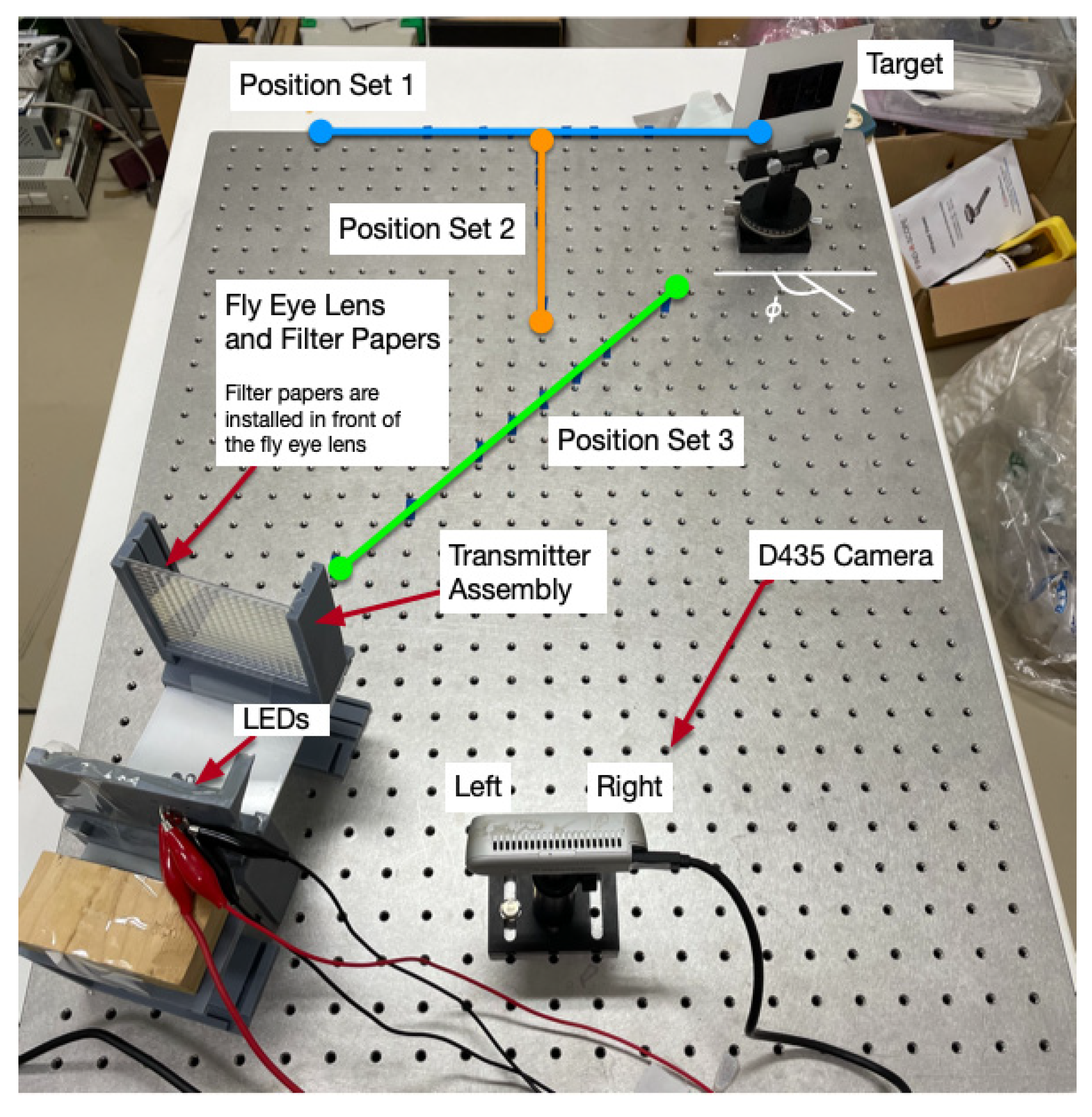
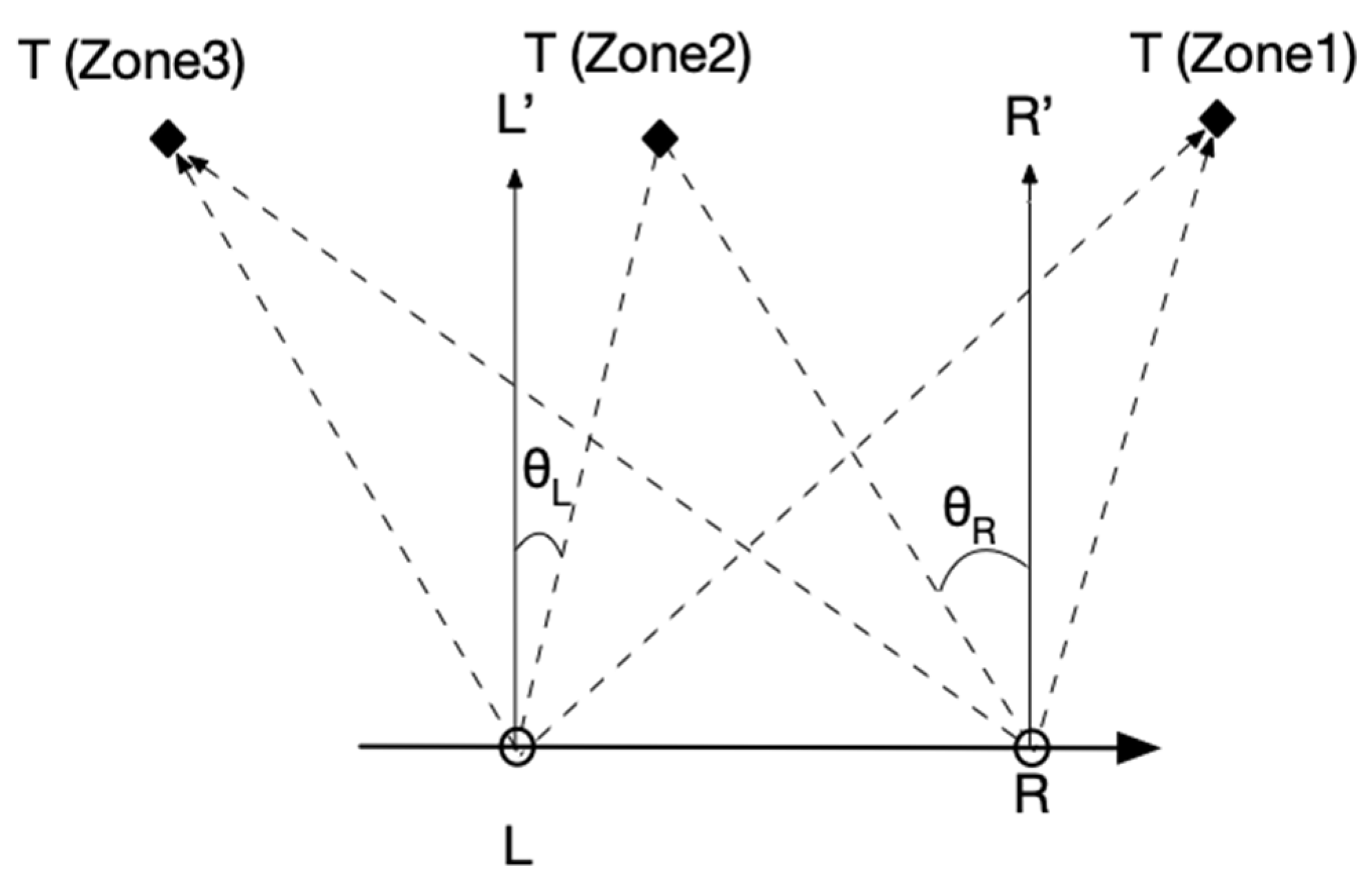
2.1. Experiment Configuration and Coordinate System

In preliminary experiments of positioning, targets were alternately illuminated by different wavelength LEDs of λ O N (850 nm) and λ O F F (940 nm), and images of these wavelengths were captured by a single camera. Figure 1 shows the layout of the experiments.
The transmitter assembly consists of 850 nm and 940 nm LEDs, both of which are two 2 mW LEDs connected in series [19,20]. To expand their beam size to be large enough to cover the target, a fly eye lens was installed in front of the LEDs. The beam divergence of the transmitter assembly was estimated to be about 85 deg (full angle, without filter paper). Even though the irradiated power control is equivalent to that of the exposure time, filter papers were introduced for independent control of the irradiated power onto the target. Power reduction by the filter paper was estimated by the brightness of the image, and it was about 50%/paper. In this report, P0 means “without any filter paper”, and P1 means “1 (one) filter paper”, etc. As for the infrared camera, an Intel D435TM depth camera [21,22] was used. Even though it can generate its own depth information, this function was not used throughout this report. Instead, both two infrared output streams of the camera were directly inputted into the image processor (PC) and processed by dedicated software. Images were captured with various exposure times. These were 25, 50, 100, 250, 500, 1000, 2500, 5000, 10,000, 25,000, 50,000, 100,000, and 200,000 μ s . The gain of the camera was set as 240, and the output image size was set to 640 × 480 px. The rest of the internal parameters were not changed from their default values. Regarding the software running on the image processor, Python [23] scripts with D435 SDK [24] and Open CV [25] were used to control the camera. For processing of the captured images, software developed by MathematicaTM [26] were used. As for target assembly, the target in the experiments of the current section was a GaAs substrate with the following specifications: manufacturer: AXT Inc. Fremont, CA, USA [27]; dopant: n-type (Si); carrier concentration: 2 ~ 3 × 10 18 c m 3 ; diameter: 2 inches; thickness: 350 μ m ; surface orientation: (001). It was on a frosted glass, and the attitude of the target was varied by rotating the stage on which it was installed. The angle of the rotatable stage ϕ increases counterclockwise and is defined as 90 degrees (deg) when the target faces normal to the camera.
There are 23 (horizontal) × 31 (vertical) screw holes on the optical bench used in the experiments, and the pitch between them is 25.4 mm. Positions of these holes were regarded as lattice points of the 2D ( x ,   y ) coordinate system on the bench, and the coordinates were defined to vary with 11   x   11 , 3   y   27 , respectively. The camera (D435) was installed at the origin (0,0), and its front face was aligned to the +Y direction. In the experiments, positions of the targets were set as follows and shown in Figure 1.
P o s i t i o n   S e t   1 = 8 ,   27 ,   4 ,   27 ,   2 ,   27 ,   1 ,   27 ,   0 ,   27 ,   1 ,   27 , 2 ,   27 ,   4 ,   27 , 8 ,   27 P o s i t i o n   S e t   2 = 0 ,   27 ,   0 ,   26 ,   0 ,   25 ,   0 ,   23 ,   0 ,   19 P o s i t i o n   S e t   3 = 6 ,   9 ,   4 ,   11 ,   2 ,   13 ,   1 ,   14 ,   0 ,   15 ,   1 ,   16 , 2 ,   17 ,   4 ,   19 , 8 ,   23
Typical parameters in this experiment are summarized in Table 1.
Figure 2 shows the procedure of generating the range information, which is the Y-coordinate of the target on the 2D plane. By differentiation and binarization of the images from the two infrared streams, target images from the left and right sensors were generated. From the center coordinates of the target detected in each image, its range was estimated from the parallax between them. Finally, the X-coordinate of the target was determined from the range and the center coordinate. The mathematical formulation of this position estimation is summarized in Appendix A.

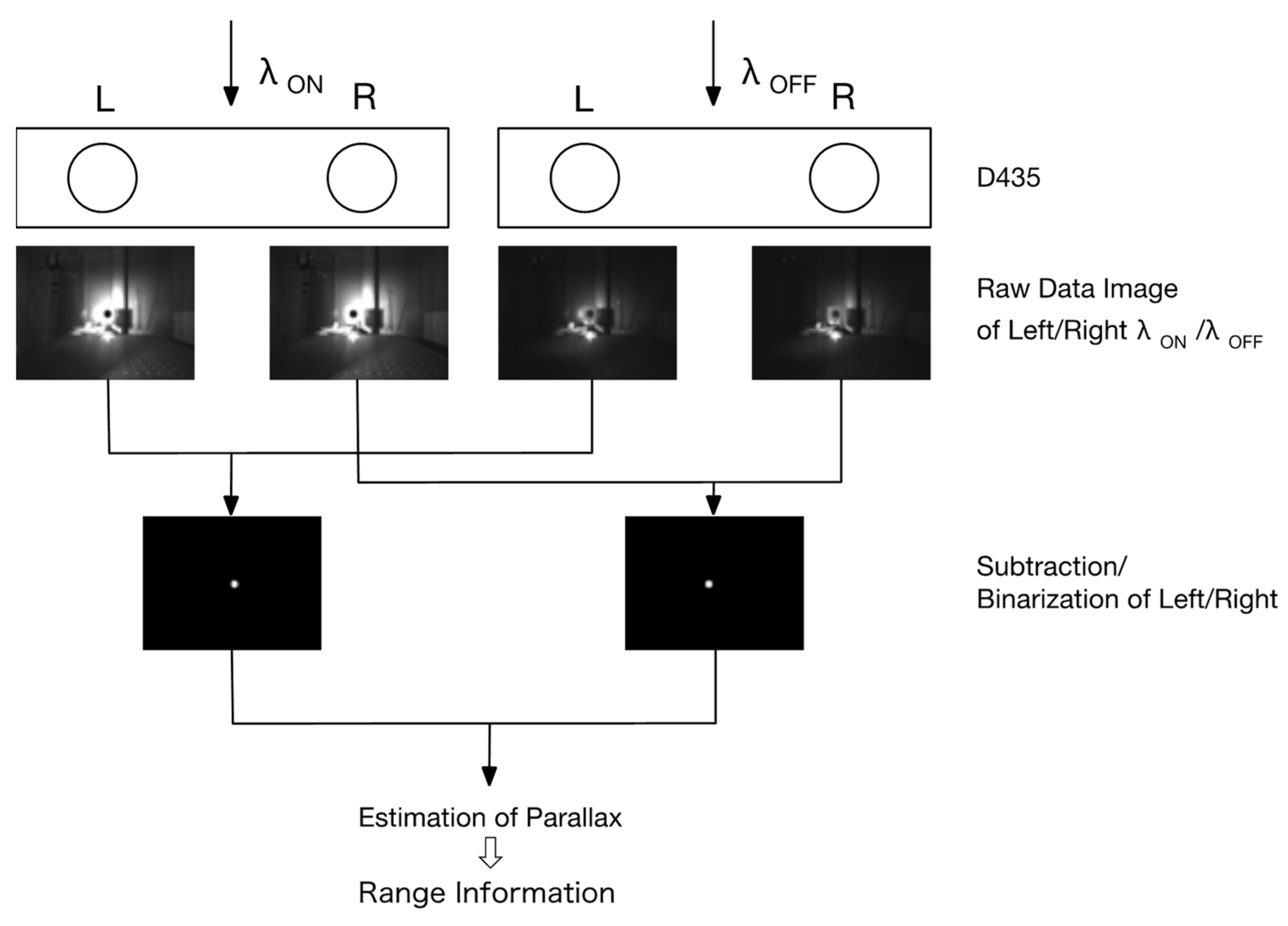
2.2. Integrity Measure

Available exposure time settings of D435 are from 25 to 200,000   μ s for its infrared streams. The accuracy of the center coordinates and the area size estimation are affected by this exposure time. To obtain a reasonable estimation accuracy, the necessary exposure time for the target should be determined. Although this depends on both the configuration and the measurement system of the experiment, a set of conditions can be defined that determines the minimum necessary exposure time. Since this is derived from the consistency consideration of the stereo imagery and it reflects the integrity of positioning, this is referred to as the ”integrity measure” in this report.
  • First condition (C1)
Figure 3 shows the target, two optical axes of the camera, and three regions in the 2D real space, with symbols representing the following: T: target; LL’: the optical axis of the left image sensor; RR’: the optical axis of the right image sensor. The plane is divided into three zones: Zone 1 is to the right of RR’, Zone 2 is between RR’ and LL’, and Zone 3 is to the left of LL’. Assume that the target is found at ξ L ,   η L and ξ R ,   η R in the pixel coordinate system of the images captured by the left and the right image sensors, respectively. Since the width of the captured image is 640 px, 0 < ξ R 320 < ξ L 320 holds in Zone1, ξ R 320 < 0 < ξ L 320 in Zone2, and ξ R 320 < ξ L 320 < 0 in Zone3. Thus, ξ L 320 ξ R 320 > 0 holds in every zone. This condition guarantees the positiveness of the estimated Y-coordinates ( y > 0 ) in Equations (A3), (A5), and (A6).
  • Second condition (C2)
Since the two optical axes of the left and the right image sensors are on the same plane, the vertical component of the center coordinate of the target detected by the left sensor is equal to the one detected by the right. Therefore, η R = η L holds. It is a necessary condition that the two coordinates determined by the left and the right sensors represent the same point of the target.
From the above discussions, the following conditions are adopted as the “integrity measure”.
C 1 :   ξ L ξ R > 0
C 2 :   η L η R = 0
In Figure 4, C1 and C2 are plotted for each position of Position Set 1 against the exposure time. The attitude angle of the target was set “Off normal(Off-axis)” ( ϕ = 110 deg) to the target to avoid excessive received power. Similar plots were obtained for both Position Sets 2 and 3 as well.
As the exposure time increases, the fluctuations in C1 and C2 rapidly disappear and both of them converge. C2 was implemented as in Equation (3), using the ”Vertical Threshold” parameter in the image processing software developed for the experiments.
η L η R V e r t i c a l   T h r e s h o l d
Figure 5 shows plots representing the relationship between the integrity measure and the estimated positioning accuracy for Position Set 1. Similar results were obtained for Position Sets 2 and 3. The vertical axis of “Mean Error” is the mean positioning error averaged over Position Set 1, and data which did not satisfy Equation (3) were removed.
Comparing Figure 4 and Figure 5, the minimum exposure time of the integrity measure convergence in Figure 4 is strongly correlated with that of the positioning accuracy convergence in Figure 5. Thus, convergence of the integrity measure can be identified as that of the positioning accuracy. Also, from Figure 5, once the integrity measure converges, the positioning accuracy is not affected by the Vertical Threshold. Since a larger value is desirable to avoid unnecessary data rejection, Vertical Threshold = 50 was set for the following discussions.

2.3. Experiments of GaAs Substrate Position Estimation

Figure 6 shows the position estimation results of a GaAs substrate for Position Sets 1, 2, and 3. Both vertical and horizontal lines are plotted using the lattice coordinates normalized by the screw hole pitch = 25.4 mm, and the solid gray dots and lines in the figures represent the true values.
Position estimation consists of range and direction estimation. The estimated direction (azimuth angle) in the 2D plane ψ defined by Equation (4) is plotted in Figure 7.
ψ = t a n 1 x y
The error limit of the estimation is defined such that the irradiated beam marginally hits the target when it is deviated an angle ε from its true value ψ (deg). Let ϕ (deg) be the target’s attitude, L be its full width, and R be its range. Then, ε can be written as Equation (5).
ε = t a n 1 d   c o s ψ + ϕ 90 R L 2   s i n ψ + ϕ 90
Let Δ x , Δ y be positioning errors, then the direction estimation error of the target Δ ψ can be expressed as
Δ ψ = y   Δ x x   Δ y x 2 + y 2
Using dimensions of the experiments in this report, Δ ψ is suppressed by the factors of order O 10 1 ~ O 10 2 . Thus, direction is more accurately estimated than range.

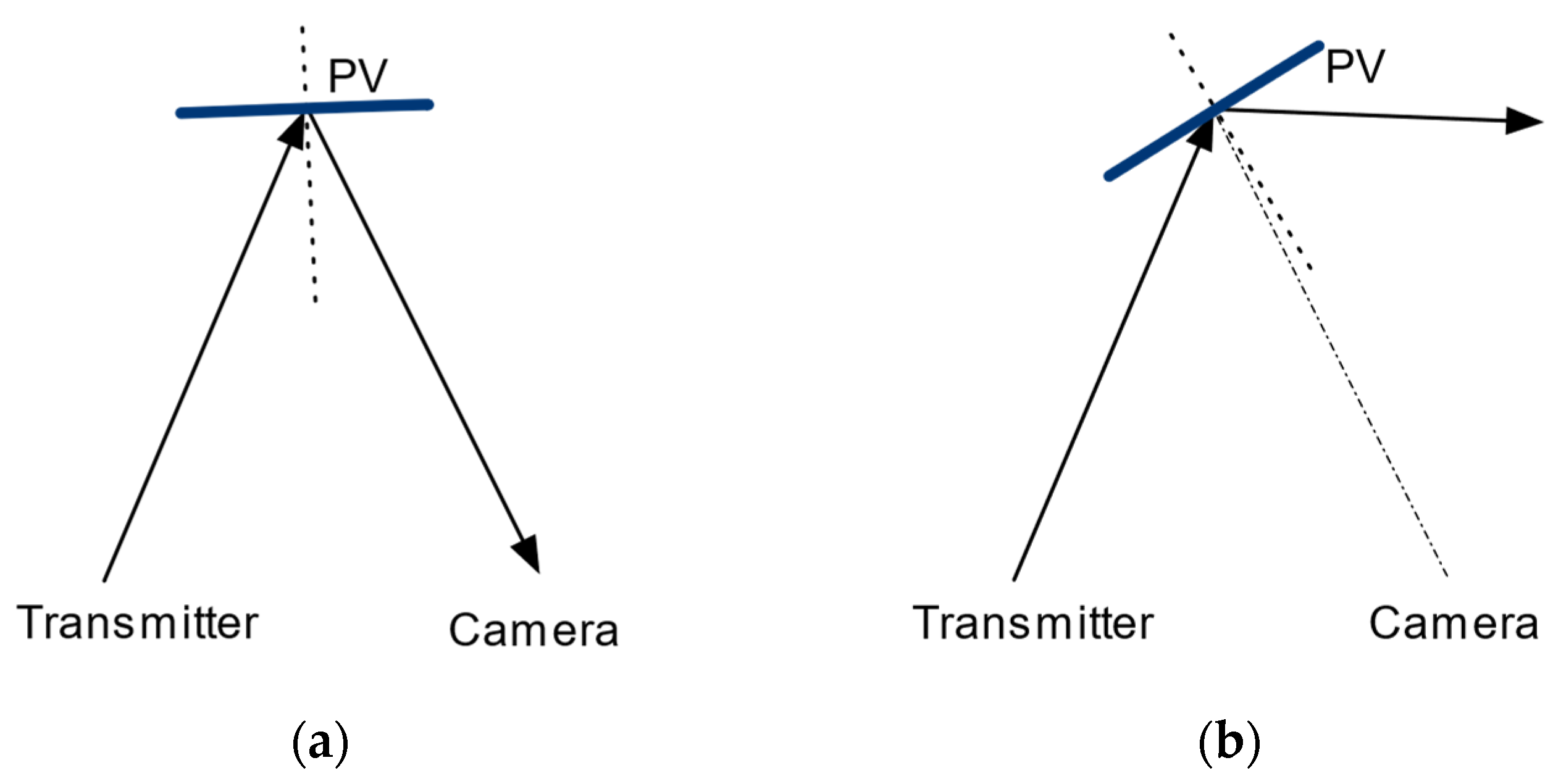
2.4. Introducing Coaxial Optics

In the experiments of Figure 1, the target was alternately illuminated by λ O N and λ O F F , and the images of these wavelengths were also alternately captured by the camera. This means that, in the case of moving targets, the target position in each wavelength image is different. To avoid this issue, the following measurement equipment with two coaxial optics was introduced into the experiments. This equipment will be advantageous for moving target detection. External views of the equipment are shown in Figure 8a,b, and the internal configuration is shown in Figure 9a,b. Two coaxial optics are included in it. After the received lights are separated into 50% and 50% by the beam splitters, λ O N   a n d   λ O F F are separated by the wavelength filters [28,29]. Figure 9a represents a left- side view of the configuration, and the reflection of the beam splitter is seen as “green” in Figure 8a. Figure 9b is a bottom view of the equipment.
The left and right image sensors of D435 (1/2) capture time-synchronized images of λ O N . D435 (2/2) captures images of λ O F F as well. Transmission efficiency of the filters was estimated by measuring the ratio of the brightness of the frosted glass image with and without the filter. Table 2 summarizes the results.
The efficiency of the coaxial optics was obtained from the value in Table 2 multiplied by the reflectance (transmittance) of the beam splitter (=0.5) and was estimated as 0.27 for λ O N and 0.135 for λ O F F . Figure 10 shows plots of the integrity measure data of the GaAs substrate experiment using the coaxial optics. Like in Figure 4, similar plots were obtained for both Position Sets 2 and 3 as well. Compared with Figure 4, the minimum exposure time of convergence for both C1 and C2 became longer. The threshold equation proposed in [15] predicts that the ratio of the convergence time in Figure 10 to those in Figure 4 gives the λ O F F transmission efficiency of the equipment. The mean value over Position Sets 1, 2, and 3 is 0.124, and this is close to the above-estimated 0.135.
The field of view (FOV) of the coaxial optics is limited by the size of the wavelength pass filters ( ϕ 12.5 mm). The FOV angle of the equipment observable by both the left and right image sensors is about 17 deg.

2.5. GaAs Substrate Experiments Using the Coaxial Optics

Positions and directions of the GaAs substrate were estimated with the coaxial optics. Like in Figure 6, the results for Position Sets 1, 2, and 3 are shown in Figure 11.
Direction estimation results are shown in Figure 12.
Position estimation accuracies degraded at both endpoints in Figure 11 due to the eclipse of the target, which is partially outside the FOV there. For other points, the results obtained for both position and direction were quite similar to those from the experiments without the coaxial optics shown in Figure 6 and Figure 7.

3. PV Positioning Experiments

Like the GaAs substrate, position and direction estimation were conducted for a GaAs PV (manufacturer: Advanced Technology Institute, Tokyo, Japan [30], five cells connected in series) using the coaxial optics equipment. For the substrate, both the center coordinates and the area size of the target could be stably estimated within a wide angular range. On the other hand, for the PV, even though estimation of the center coordinates was available within a wide angular range, the area size estimation was limited to within the neighborhood of its normal. Such a difference affects the position determination characteristics of the PV, which are different from the substrates as described below.

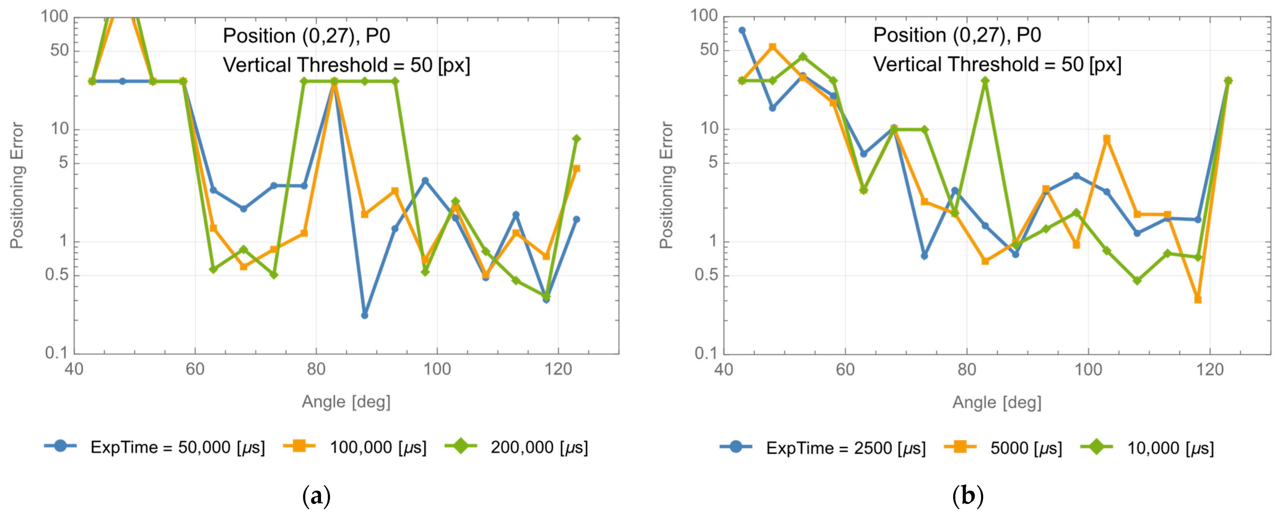
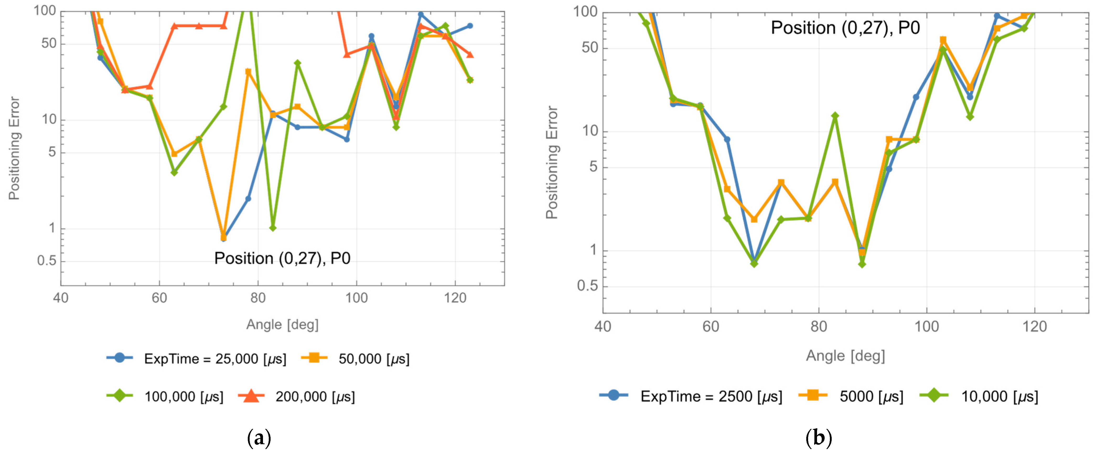
3.1. Positioning of the PV at (0, 27)

Position estimation was conducted with a fixed target at (0, 27) for various ϕ . Results are shown in Figure 13. Positioning errors for each axis are expressed as Δ x , Δ y , and Δ x 2 + Δ y 2 are plotted with ϕ as the horizontal axis. It decreases in the range 78   ϕ     98 deg and rapidly increases in both outer sides.
Figure 14 shows the angular characteristics for determining the center coordinates and the area size in the pixel coordinates of the image sensor, based on the data from the previous report. The plots show the angular dependence of the minimum exposure time (vertical axis) for determination of the X and Y center coordinates and the area size.
Figure 14a indicates that the center coordinates of the substrate are stably determined in a wide angular range. On the other hand, regarding the minimum exposure time for detection of the center coordinates of the PV, Figure 14b shows that the value around the neighborhood of the normal differs from the one outside of it. For the positioning of the PV, determination of the X-coordinate of its center is necessary. The resultant positioning accuracies of the PV reflects this steep angular characteristic of the X-coordinate determination, and this implies that positioning accuracies are strongly affected by the reflection characteristics of the targets.
Figure 15 shows the results of a similar experiment in which the coaxial optics were removed to increase the power received by the camera. As explained in Section 2.4, the received power differs by about 8-fold between Figure 13 and Figure 15. Comparing Figure 13 and Figure 15a, positioning accuracies were improved at both sides of the 78     ϕ     98 deg range. Even though they were degraded around the range, however, from Figure 15b, this can be avoided by limiting the exposure time appropriately. Thus, as a whole, positioning accuracy can be improved in the 63   ϕ   118 deg range by increasing the received power.

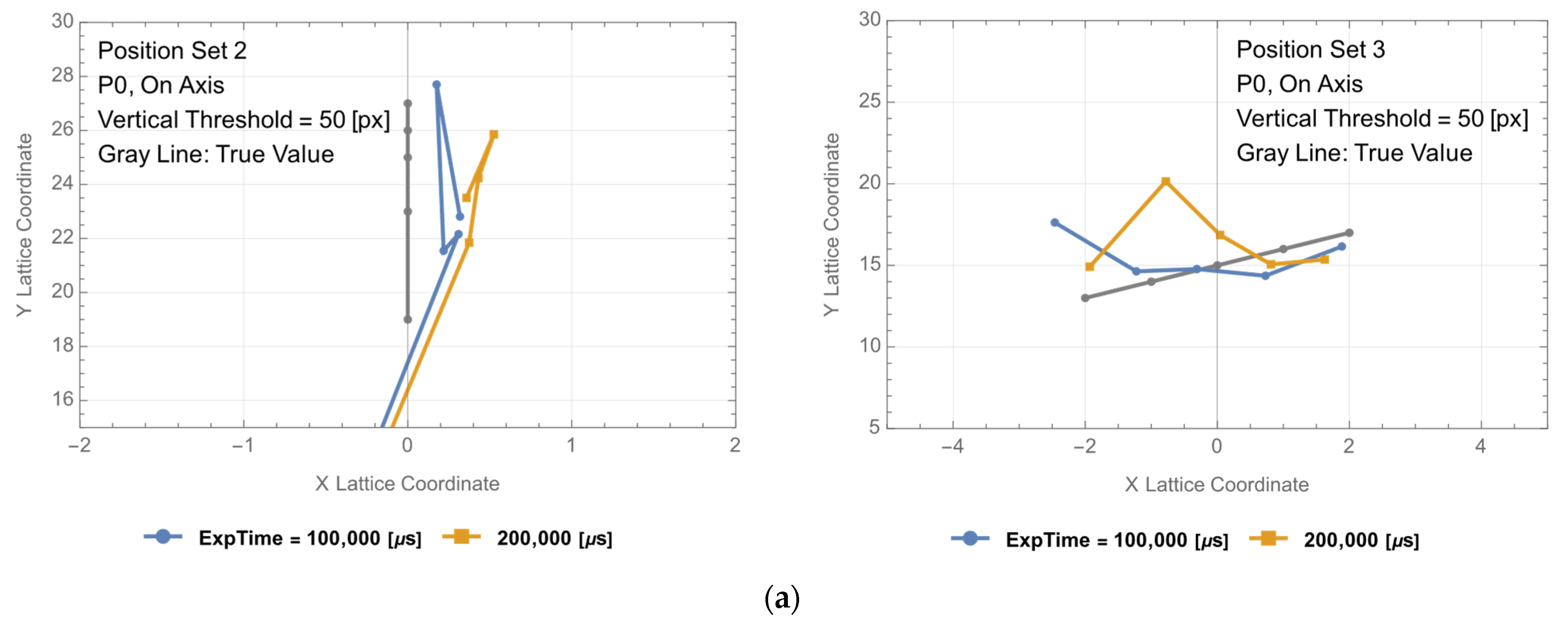
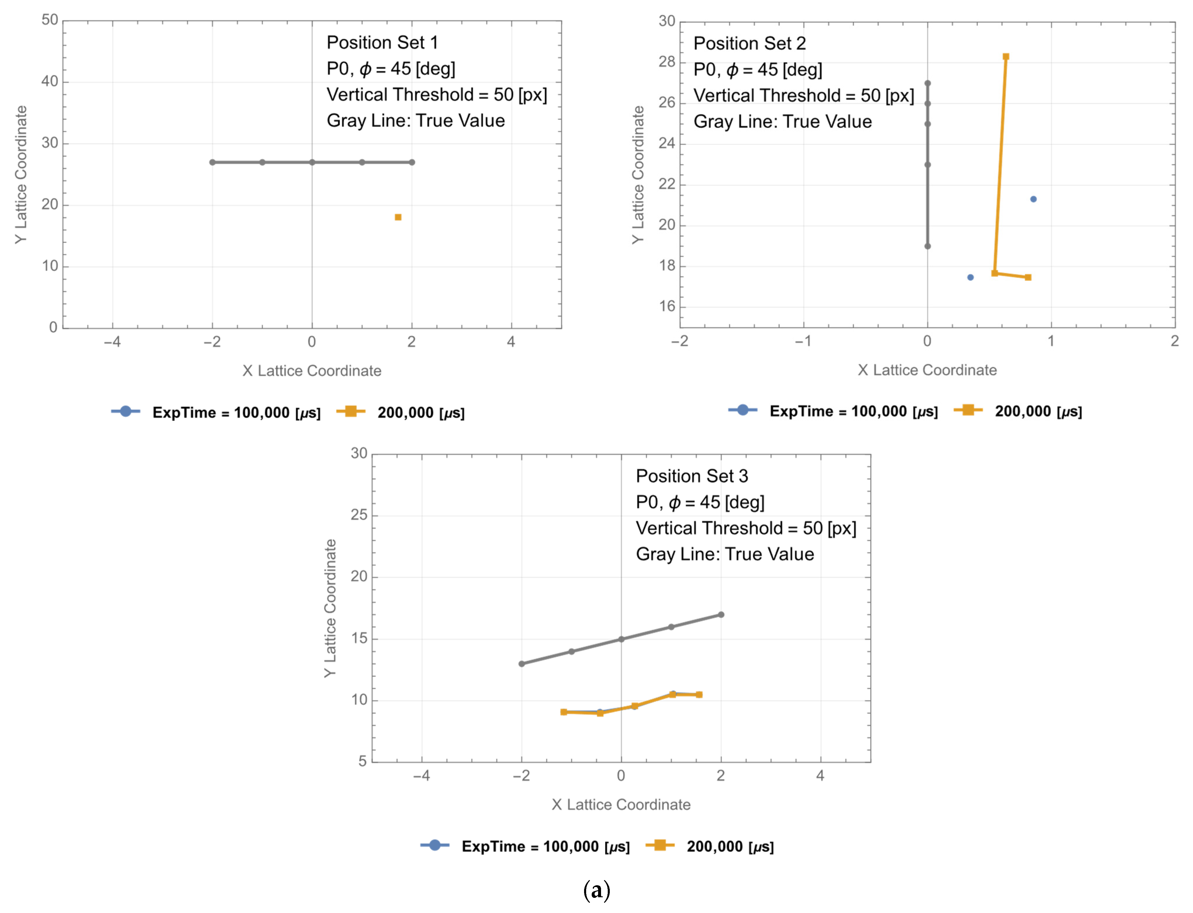
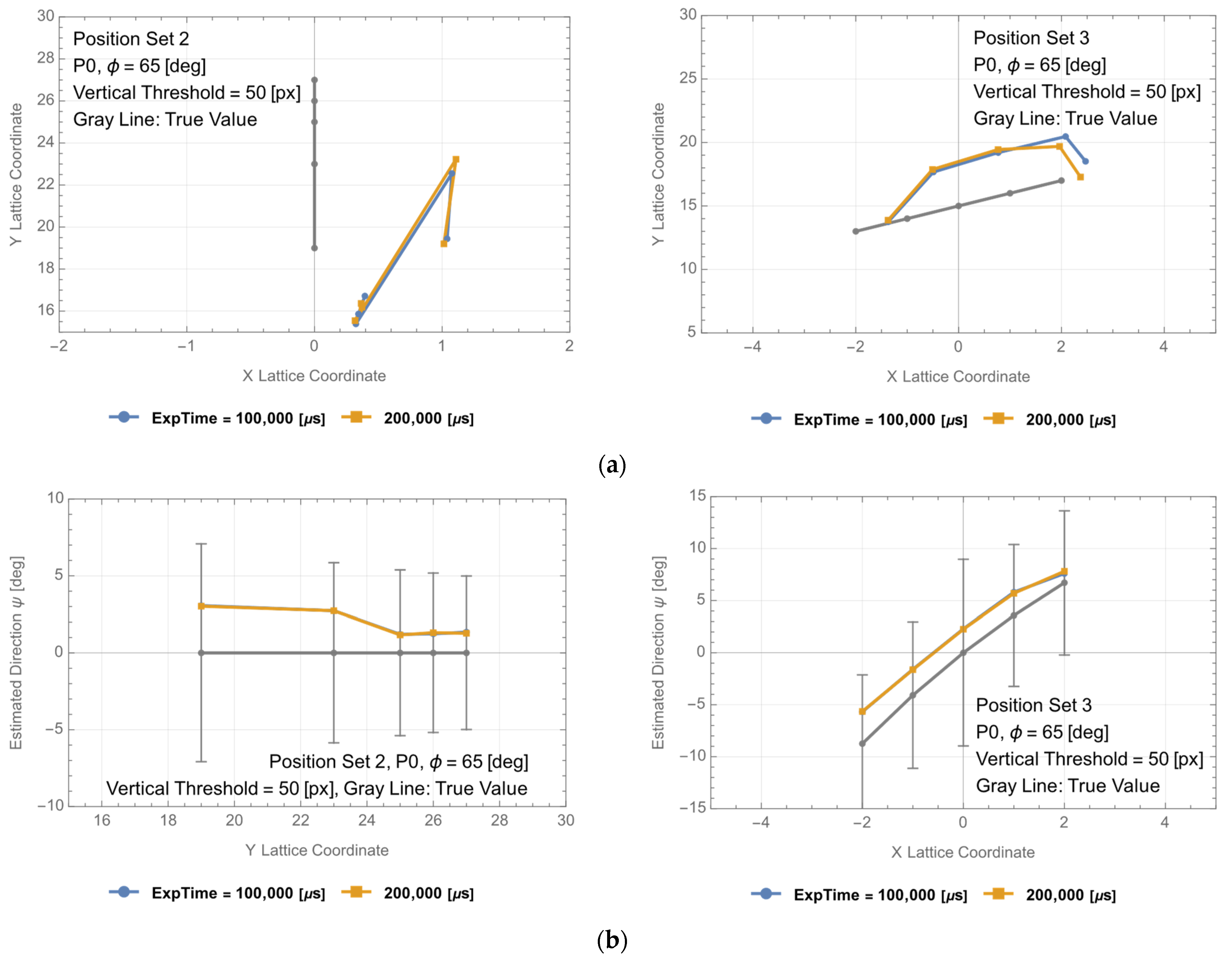
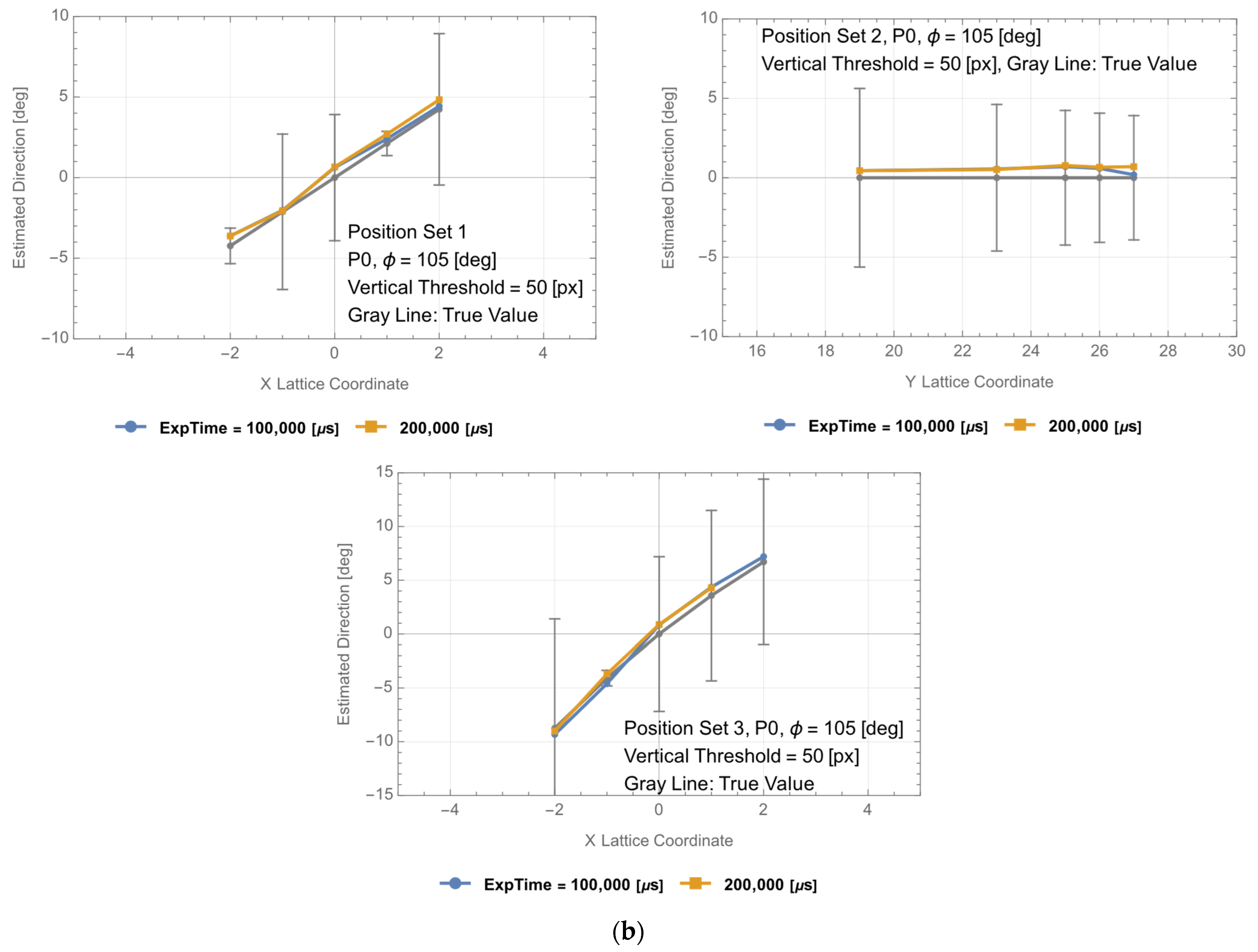
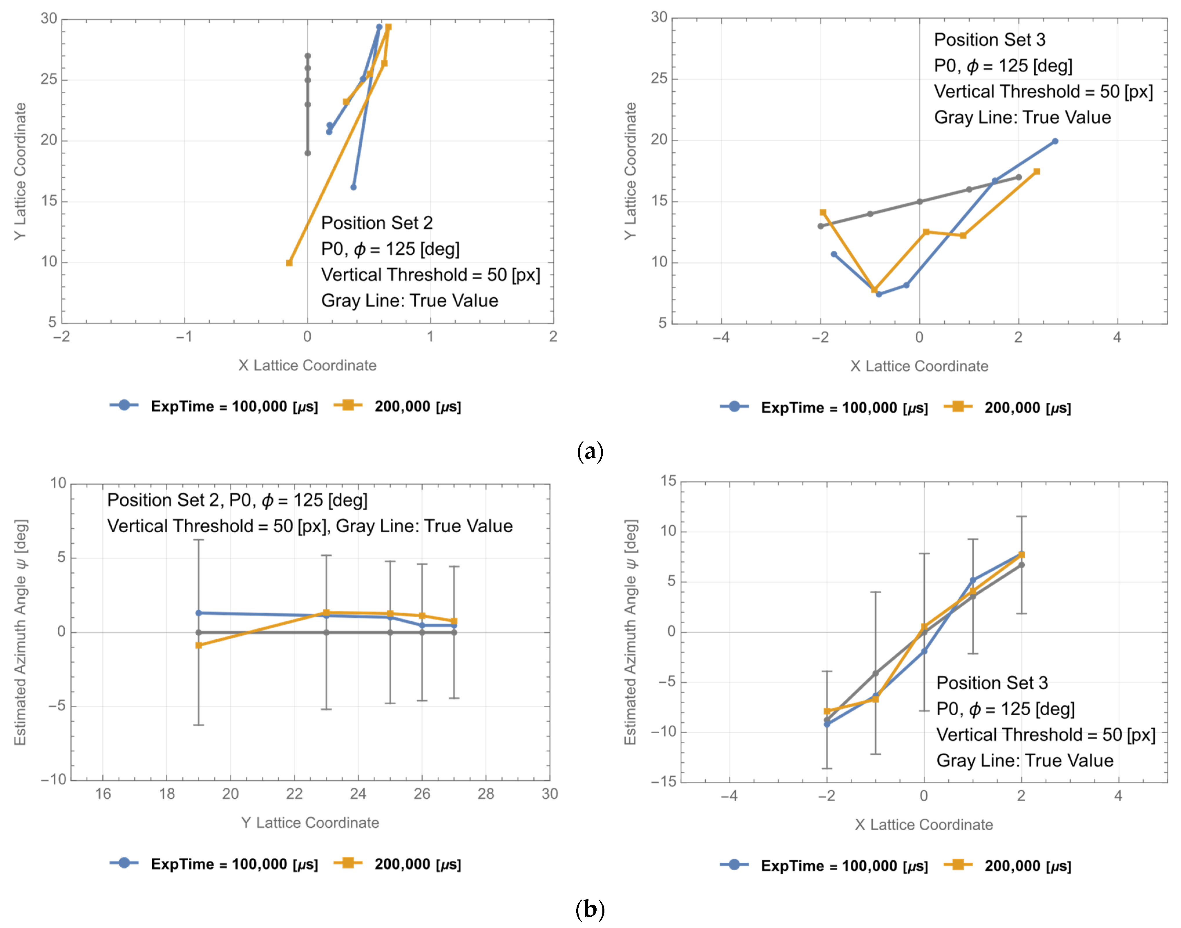
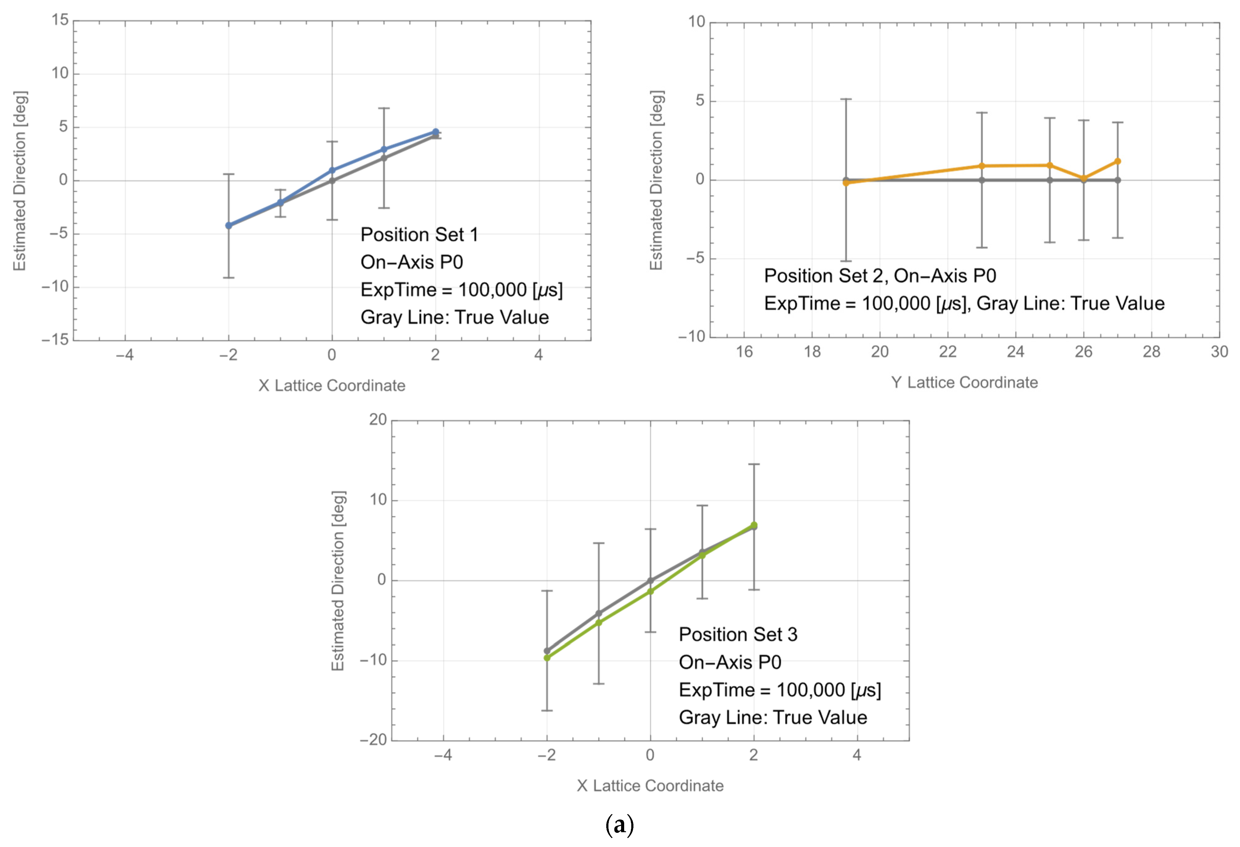
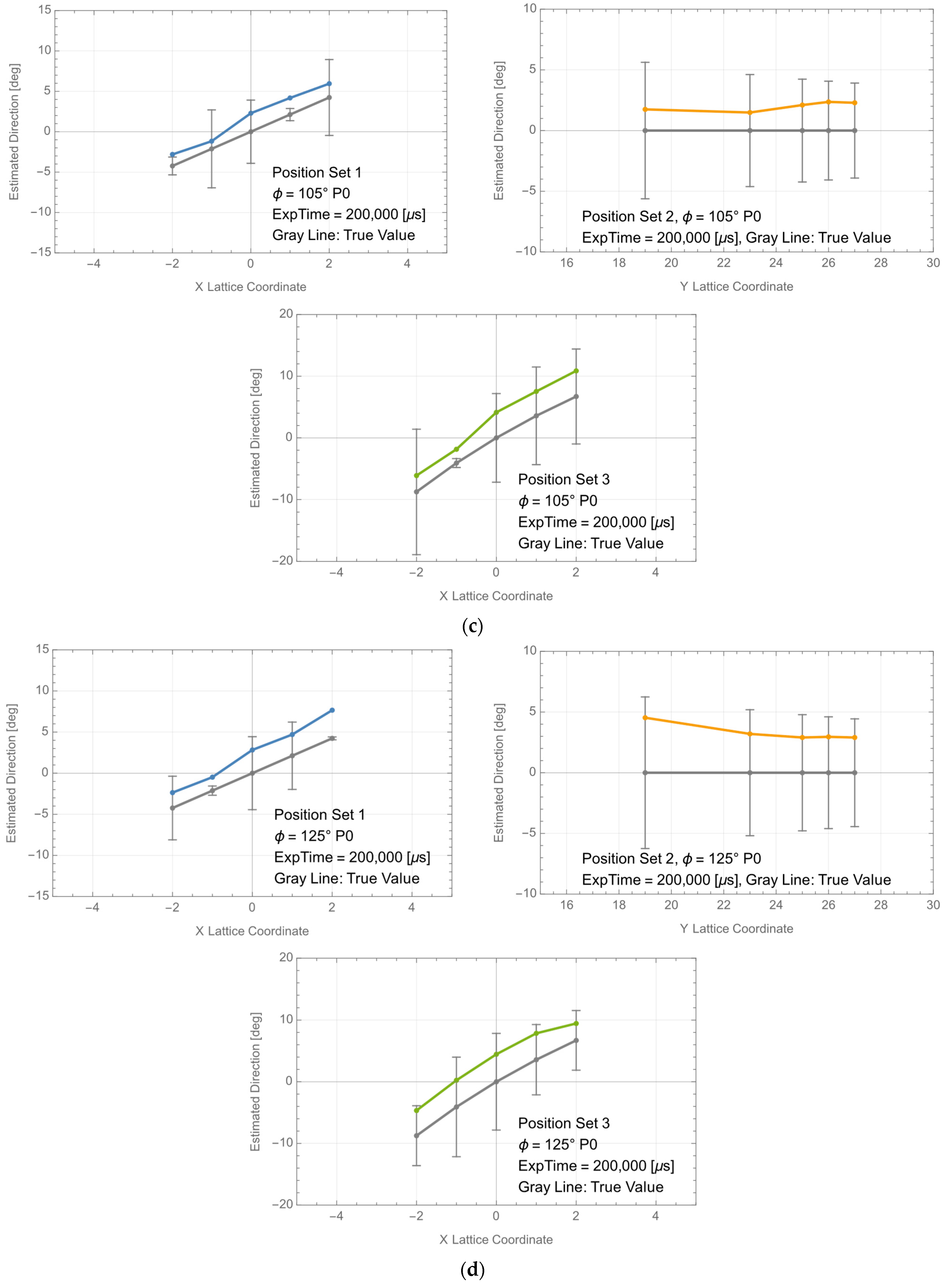
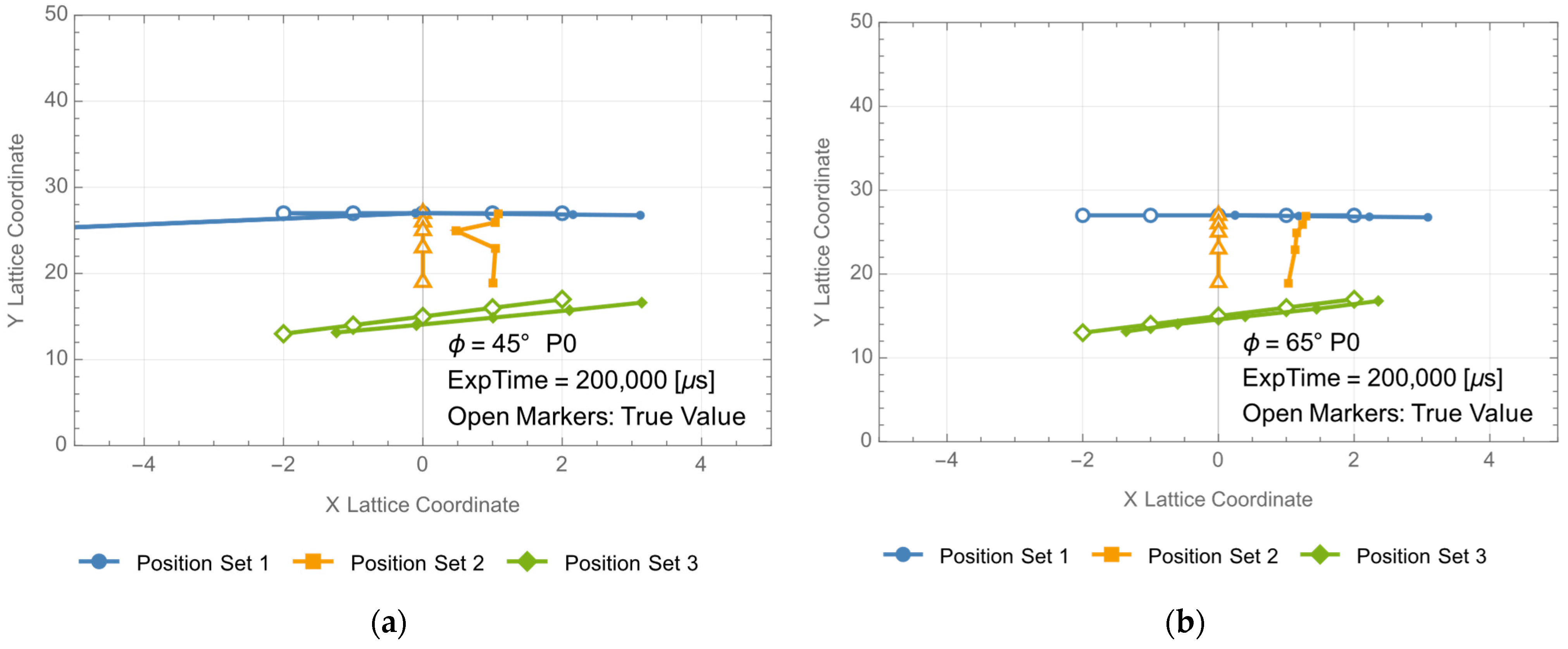
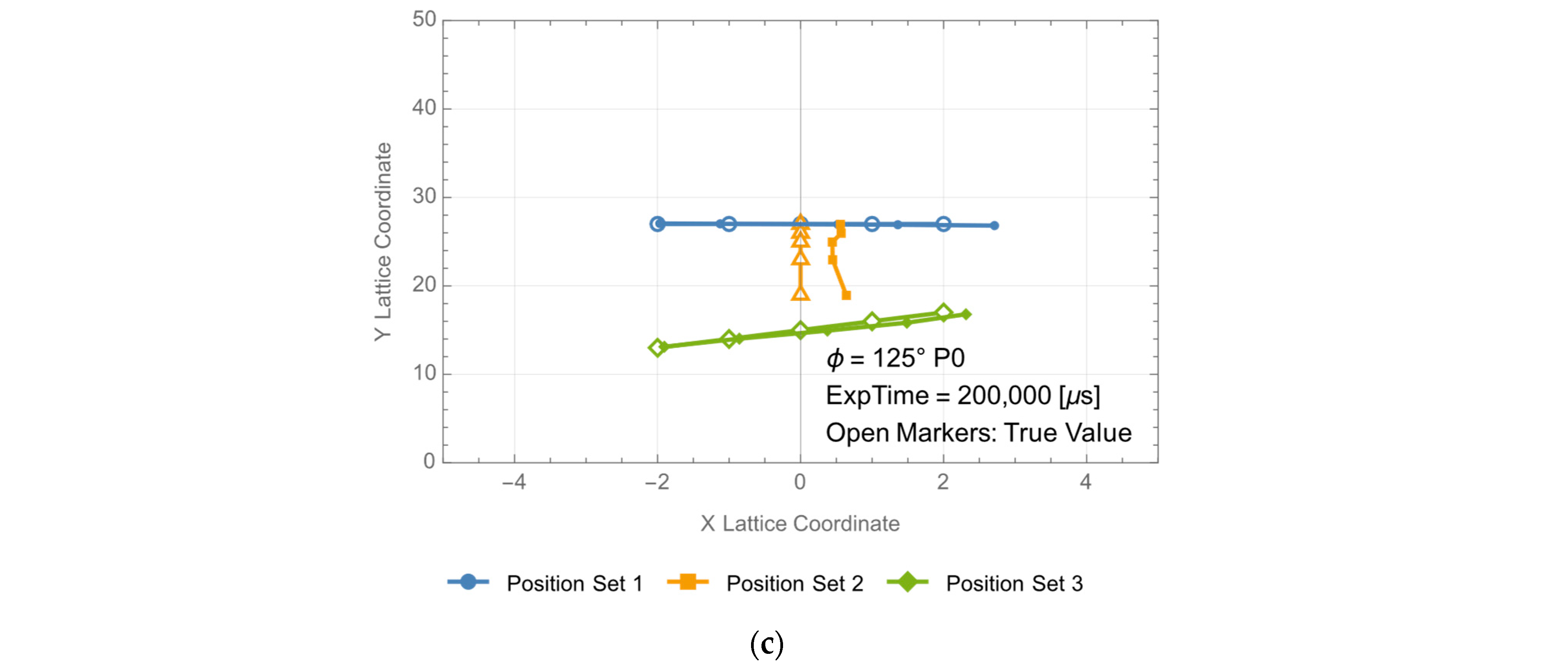
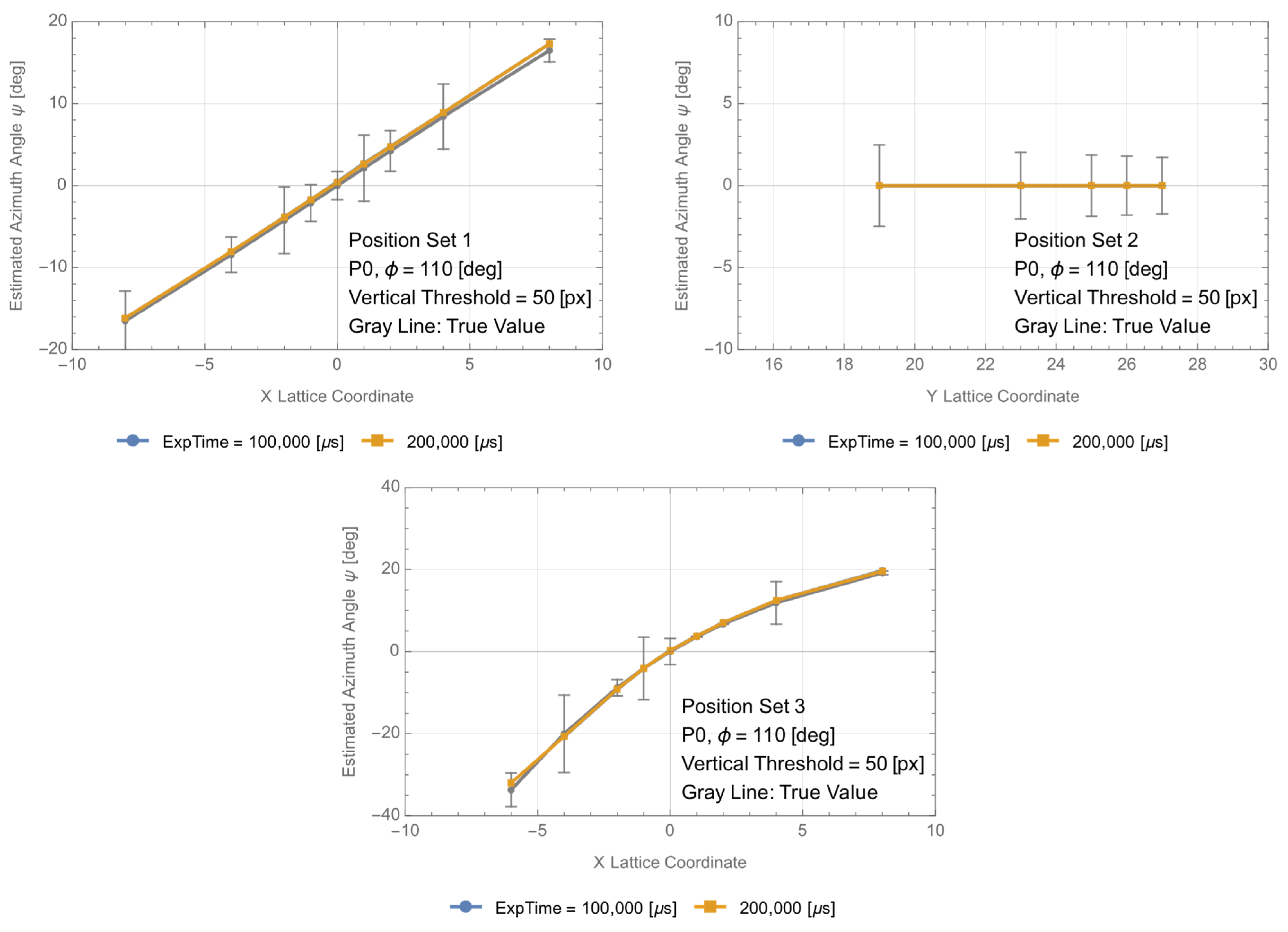
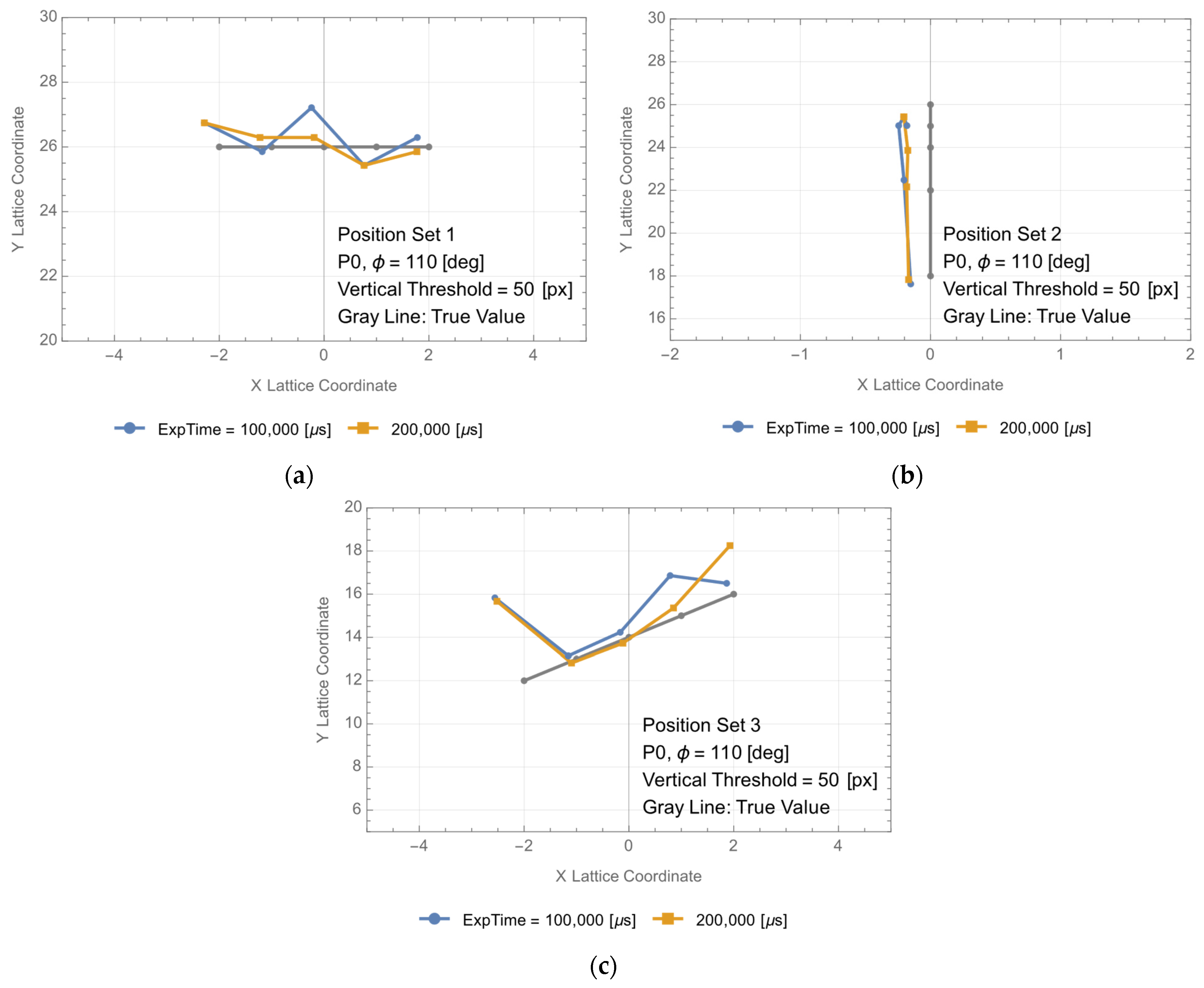
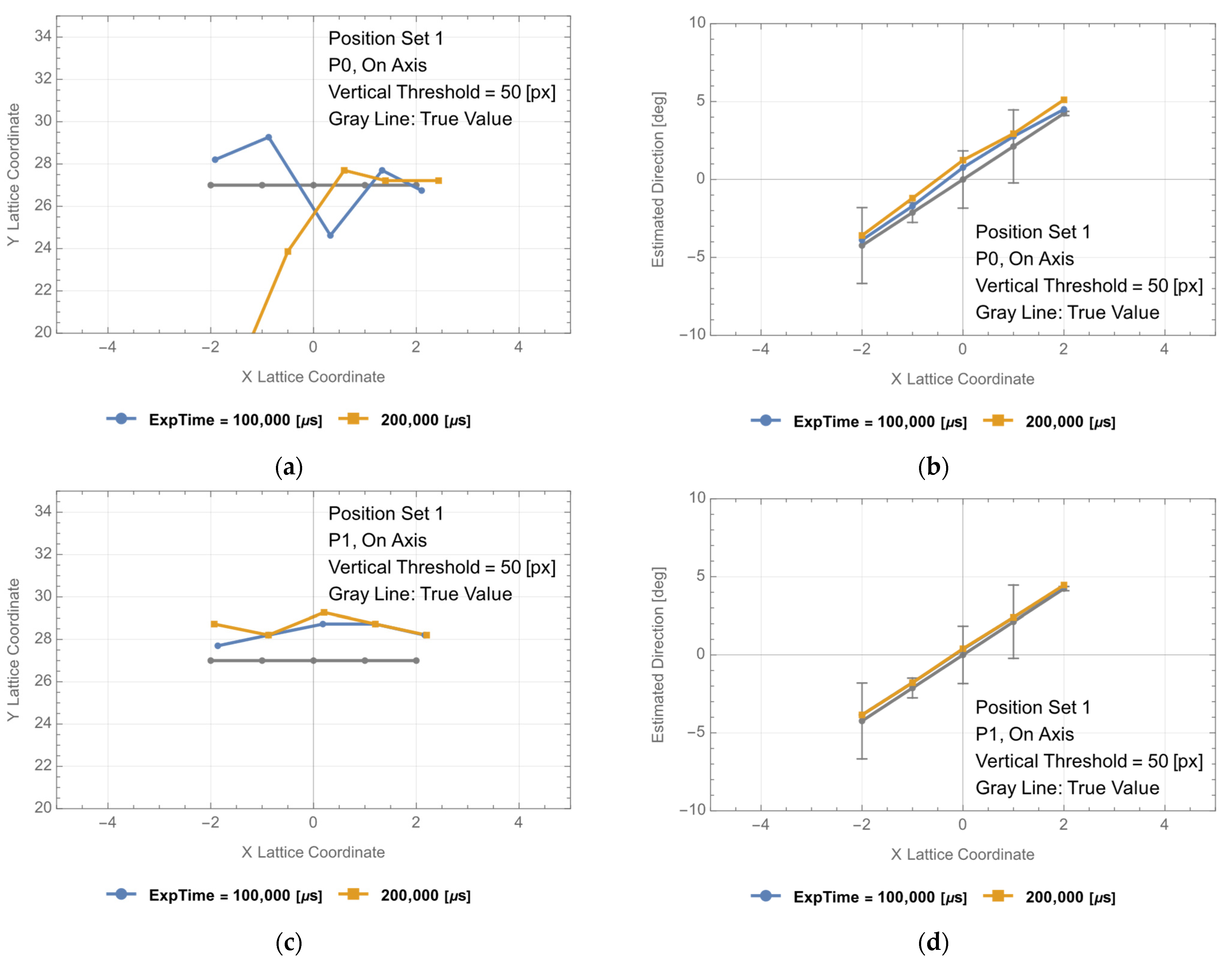
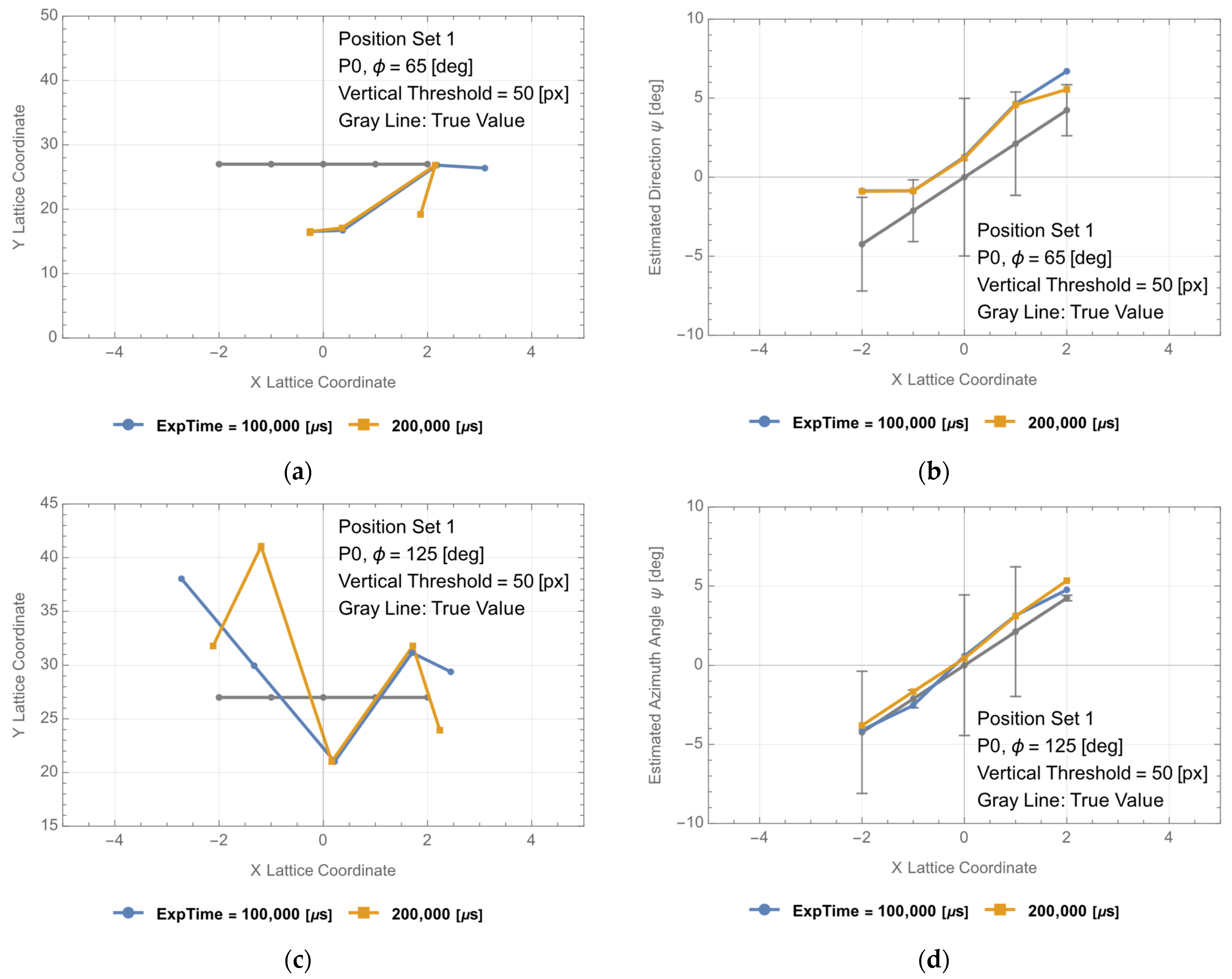
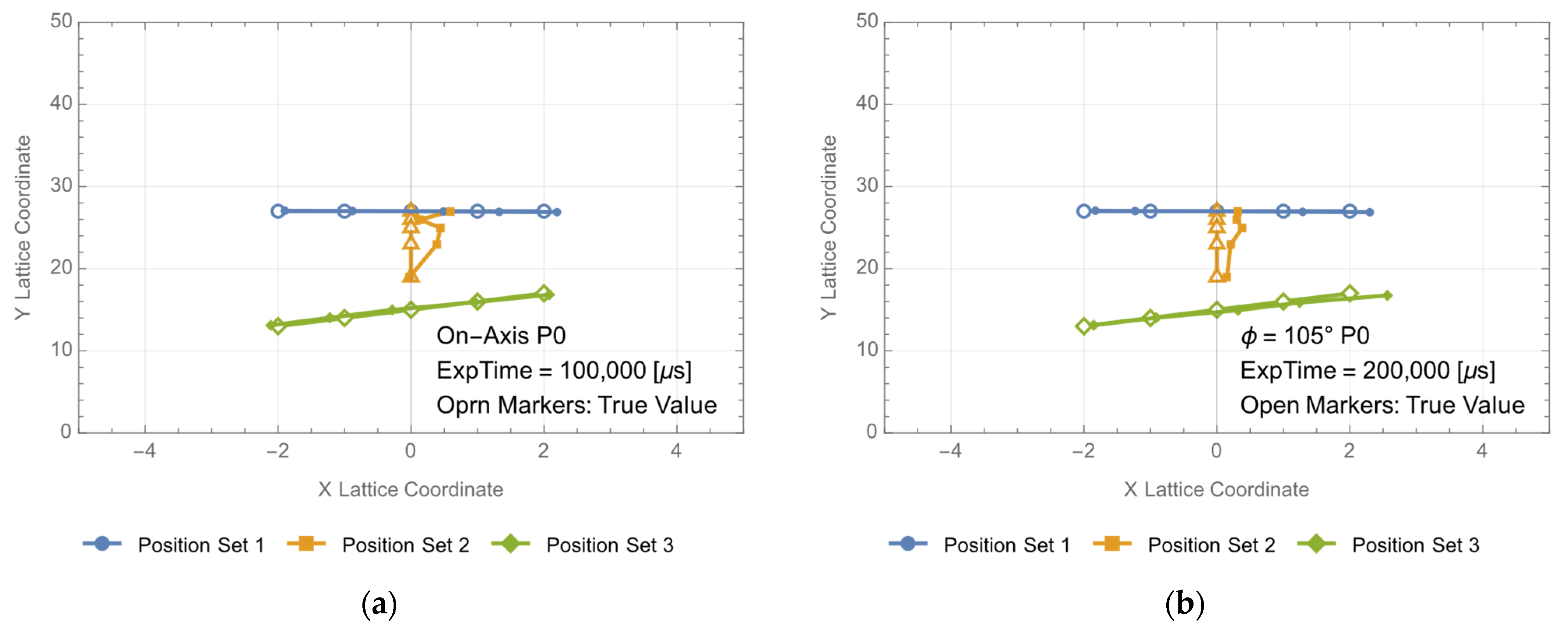
3.2. Positioning of the PV at Position Sets 1, 2, and 3

In the experiment with the substrate, the angle of the rotatable table (=attitude angle of the target) was ϕ   = 110 deg. Considering that the irradiated beam is reflected by the target and directly enters the camera, like in Figure 16a, its attitude angle ϕ depends on the position and satisfies Equation (7).
ϕ = c o s 1 P + B · N P + B N
where P is the position vector of the target, B is the directional vector of the irradiated beam, and N is the directional vector of the camera facing normal. This angle ϕ is referred to as the “on-axis angle” throughout this report.
Using the lattice coordinates and from the experiment layout, B = 1,4 and N = ( 0,1 ) . The on-axis angle distributes from a 79 deg to 87 deg angular range for the target in Position Sets 1, 2, and 3. Two kinds of experiments were conducted for the PV. One was where ϕ was always adjusted to the on-axis angle of the target’s position, which is referred to as the “on-axis experiment”. The other was like in Figure 16b, where ϕ was fixed at the same angle, which is different from the on-axis angle. This is referred to as the “off-axis experiment”.
Some results of the on-axis P0 and P1 GaAs PV position estimations are excerpted and shown in Figure 17. The rest are summarized in Appendix B.1.
Even though the directions were stably estimated like in Figure 12, degraded results of position accuracies were obtained for every position set for P0. In the P0 on-axis experiments, the light input to the camera is excessive and, due to scattering by the filter holder and partial saturation of the image at the sensors, this causes accuracy degradation. These issues were relaxed in P1, and its actual accuracies were better than those of P0. Off-axis experiments were conducted by varying the attitude angle ϕ (referred to as the “off-axis angle”) to 45, 65, 105, or 125 deg. Some results are shown in Figure 18. The rest are shown in Appendix B.2.
Since the layout in Figure 1 was asymmetric with regard to the optical axis of the camera, accuracies at ϕ = 105, 125 deg were better than those at ϕ = 45, 65 deg. Compared with the on-axis experiments, accuracies were degraded in the off-axis case. In contrast, from data in Appendix B.1 and Appendix B.2, the estimated direction is within the requirements, at least in the 65   ϕ   125 deg range, and it can be determined in more than a 60 deg full angular range even in off-axis conditions. Since the results of the on-axis and off-axis experiments are qualitatively consistent with Figure 13, the figure can be regarded as representative data of the on-axis and off-axis experiments, and the discussion in Section 3.1 also holds for the results in this section.
In the substrate experiments in Section 2.4, the attitude angle was ϕ = 110 deg. Comparing results of the substrate experiments with the PV results ( ϕ = 105 deg), even though the attitude angles of these two are close to each other, the positioning accuracies are better in the substrate experiments, in which the reflection characteristic is mainly diffuse, than in the PV case, which is mainly specular.

4. Discussion

In OWPT, position determination of the PV strongly affects the design and operation of the system. In stereo imagery, since the necessary width between left and right sensors is proportional to the range of the target, the size of the image sensor unit would be an issue for a distant target. In the case that the range is determined by another method, the issue would be diminished. Assuming the target size is known, its range can be estimated by measuring its apparent size. This method was investigated using data from the right image sensor and sizes of the target (substrate: ϕ 50 mm, PV: 60 mm × 40 mm). Estimating direction using the same data, the position was then determined by these two factors. The mathematical formulation is simple, and it is included in Appendix A.3.

4.1. GaAs Substrate

Results of the position and direction estimations are shown in Figure 19 and Figure 20.
Comparing these figures with Figure 11 and Figure 12, these results are similar to them. In the substrate experiments, the performance difference between the stereo imagery and the apparent size method is small.

4.2. GaAs PV

4.2.1. Positioning of the PV at (0, 27)

Like in Figure 13, the position of the target fixed at (0, 27) was estimated with the attitude angle as the horizontal axis. Results are shown in Figure 21.
The position error decreases within the 63   ϕ   88 deg range and rapidly increases outside of it. The full width of the angular range is 25 deg, which is also close to the full angular width of the area size determination in Figure 14b. This is because the vertical target size was used in Figure 21, and capturing whole (vertical) image of the target is necessary to estimate it. Like in Figure 15, position estimation results for the fixed target at (0, 27) without the coaxial optics are shown in Figure 22.
Even though some accuracy improvements can be seen on both sides of the on-axis angle in this case as well, compared with those in Figure 15, the improvements in Figure 22 are limited. This can be explained by a similar discussion to the one in Section 3.1. Generally, increasing the received power is equivalent to increasing the irradiated power, etc. [15]. In this case, it is equivalent to increasing the exposure time in Figure 14. In Figure 13, stereo imagery positioning was based on estimation of the X-coordinates of the target, and this corresponds to the X-coordinate plot in Figure 14b. In contrast, Figure 22 is based on area size estimation, and this corresponds to the area size plot in Figure 14b. Even though the angular characteristics of the area size and the X-coordinate are similar in the neighborhood of the normal, they are quite different outside of it. Thus, the angular characteristic related to area size that is shown in Figure 21 is different from that of Figure 13 that is related to the X-coordinate.

4.2.2. Positioning of the PV at Position Sets 1, 2, and 3

Excerpted on-axis results are shown in Figure 23a. The rest are included in Appendix C.1. The off-axis results are shown in Figure 23b,c and Appendix C.2. Comparing these results with Figure 17 and Figure 18, like in the substrate experiments, the two methods provided similar results also for the PV. Like in Section 3.2, these results are consistent with Figure 21, and it can be regarded as representative data of the on-axis and off-axis experiments.
Close investigation and comparison of the positioning error between the stereo imagery and the apparent size measurement show that their angular characteristics are similar in the on-axis neighborhood and different in the off-axis range. In Equation (8), the position estimation error Δ x 2 + Δ y 2 is expressed using 2D polar coordinate variables (range R , azimuth angle (direction) ψ ) and their errors ( R , ψ ).
Δ x 2 + Δ y 2 = R 2 + R   ψ 2
ψ can be compared between the stereo imagery off-axis data (Figure 18b,d, Figure A6, Figure A7, Figure A8 and Figure A9) and the apparent size measurement (Figure A13). Table 3 summarizes the result for Position Set 1, in which the typical value of R = 27 is used.
Comparing these R   ψ estimations with the position estimation error of the stereo imagery (Figure 18a,c, Figure A6 and Figure A8) and the apparent size measurement (Figure 23b,c), Δ x 2 + Δ y 2 R   ψ always holds, which means that R , instead of R   ψ , dominates the position estimation error. In the apparent size measurement, the off-axis position estimation error of Position Set 1 is so large that some of them are beyond the plot range ( ϕ = 45, 105, 125 deg). In the stereo imagery, the errors are still large but within a 5 to 20 unit range, except for ϕ = 45 deg. This observation indicates that the off-axis positioning errors are affected by the off-axis R , which differs between the stereo imagery and the apparent size measurement, as discussed in Section 4.2.1.
Comparing the on-axis case of the stereo imagery (Figure 17a,c) and the apparent size measurement (Figure 23a and Figure A10), all the data support Δ x 2 + Δ y 2 ~ O ( R   ψ ) . This means that R values are small enough and of the same order as R   ψ . This observation is consistent with the results of the fixed-point positioning in Figure 13 and Figure 21.
The difference in the position estimation error in these two methods appears in the off-axis angle range and suggests that it is strongly affected by the shape of X-coordinates estimation and area size estimation in Figure 14b. For Position Set 2 and Position Set 3, the same results are obtained.

4.2.3. Position Estimation with External Ranging Information

If the exact range data are provided externally, there would be an option to determine the target’s position based on range information from the external ranging source combined with the internally estimated direction. In fact, the dominant contribution to the positioning error is removed by setting R = 0 in Equation (7). Position accuracies were estimated using (exact) range information with the internal direction estimation. Results are shown in Figure 24 and Appendix D. In this case, accurate positioning results were obtained for both on-axis and even for off-axis conditions.

5. Conclusions

Position estimation by means of differential absorption imaging in OWPT was investigated using two methods. One was the stereo imagery method. The other was based on range estimation by the apparent size of the target combined with direction estimation. For the stereo imagery, in the GaAs substrate experiments, position determination is not strongly affected by its attitude angle. In contrast, in the GaAs PV case, results were quite different between the case where the target attitude was set so as to reflect the irradiated beam directly to the camera (on-axis) and the case where its attitude was set so as not to do so (off-axis). This is consistent with the angular characteristics of the center-coordinate determination of diffuse and non-diffuse targets in the previous report. For the method using apparent size, position estimation is evidently affected by characteristics of the area size determination. On the other hand, estimation of direction is not strongly affected by the attitude of the target, and it is available for a wide angular range of nearly 90 deg.
One of the necessary conditions of position estimation for both methods is that, ideally, the entire image of target is clearly captured. However, according to previous research, this is not always available, especially for tilted targets. Thus, in this report, position was estimated using the center coordinates of the boundary rectangle of the captured target. In the case of estimation by stereo imagery, a condition which is referred to as the “integrity measure” can be defined to avoid inconsistencies between images captured by two optical sensors. Instead of capturing the entire image of the target, this is a necessary condition for accurate positioning in the stereo imagery for the differential absorption imaging.
Regarding the ranging accuracy, both methods were affected by the relative attitude of the target to the receiver optics. The 2D position of the targets was estimated to within a 1-unit error in both methods (1 unit = 25.4 mm) when it faced normal to the optics. Positioning accuracies in both methods were degraded to a few tens of units with an attitude angle deviation from the normal; this angle allowance is 25 to 30 deg in the GaAs PV, which has mixed reflection characteristics. Also, it was found that by increasing the received power 8-fold, this angle characteristic was relaxed, and accuracy was improved. In contrast, the direction estimation was more stable with attitude angle variations than the position estimation.
In the case where the attitude angle deviation from the normal of the target is more than 20 deg, and its range estimation is difficult from the transmitter, there would be two strategies for obtaining position coordinates. One is that the transmitter sends direction data to the receiver; then, the receiver controls its attitude by itself. This is applicable to a system which has a cooperative relationship between the transmitter and the receiver (cooperative OWPT) [9]. Another strategy is that transmitter obtains ranging information from equipment such as a laser range finder and estimates the position with direction information obtained itself. Both options utilize the fact that direction estimation is more stable than that of range in response to attitude angle variation.
There have not been many studies about the detection and positioning of targets in the OWPT system. In this report, a basic study was conducted. For both the cooperative and non-cooperative OWPT beam alignment and shaping discussed in [9], this study provides a basis for the early phase of their operation.

Author Contributions

Conceptualization, K.A. and T.M.; methodology, K.A. and T.M.; formal analysis, K.A.; investigation, K.A.; data curation, K.A.; software, K.A.; writing—original draft preparation, K.A.; writing—review and editing, T.M.; project administration, T.M.; funding acquisition, T.M. All authors have read and agreed to the published version of the manuscript.

Funding

This work was partially supported by the Tsurugi-Photonics Foundation (No. 20220502) and the Takahashi Industrial and Economic Research Foundation (No. I2-003-13). In addition, part of this paper is based on the project commissioned by the Mechanical Social Systems Foundation and Optoelectronics Industry and Technology Development Association (“Formulation of strategies for market development of optical wireless power transmission systems for small mobilities”).

Institutional Review Board Statement

Not applicable.

Informed Consent Statement

Not applicable.

Data Availability Statement

Not applicable.

Acknowledgments

The authors thank Kenta Moriyama, members of the T. Miyamoto Lab for discussion and assistance, and Yota Suzuki of the Open Facility Center of Tokyo Institute of Technology for design support and manufacturing of the equipment for the experiments.

Conflicts of Interest

The authors declare no conflict of interest.

Appendix A. Mathematical Formulation of PV Positioning

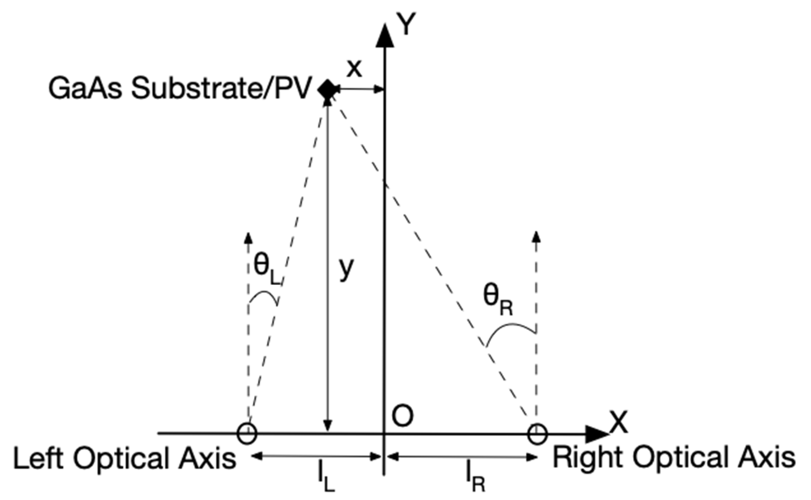
Appendix A.1. Positioning Formula with Stereo Imagery

Cartesian X, Y, Z axes are defined in real three-dimensional (3D) space as Z = X × Y , and their coordinates are defined as (x, y, z). Assume that the two optical axes of the left and the right image sensors are parallel with each other and that both optical axes are included in the XY plane. Also, assume that the left optical axis and the right optical axis are parallel with the Y-axis. Then, consider that the target is projected onto the XY plane. Lengths and angles in the XY plane are defined as in Figure A1.
Figure A1. Configuration of positioning (stereo imagery).
Photonics 10 01111 g0a1
l L = y   t a n θ L
l R = y   t a n θ R
From Figure A1, since Equations (A1) and (A2) hold, coordinates of the target (x, y) are expressed as
y = l L + l R t a n θ L t a n θ R
x = y t a n θ L l L
Both l L   a n d   l R are known parameters and, according to the datasheet of D435, their values are 17.5 mm and 32.5 mm respectively. The image size from D435 was set to 640 × 480 px. The origin of the pixel coordinate system of both image sensors is defined as the bottom-left corner, and pixel coordinates ( ξ ,   η ) are defined as 0   ξ   639 , 0   η   479 . From Equation (2), the left/right vertical pixel coordinates should be the same ( η L = η L η ) , and we assume that the pixel coordinates of the target are ξ L ,   η ,   ξ R ,   η in the left and the right sensors respectively. Then θ L ,   θ R are given by Equations (A5) and (A6).
θ L = t a n 1 θ ξ L 320
θ R = t a n 1 θ ξ R 320
From Equations (A3)–(A6), (x, y) can be expressed as follows, where θ converts the pixel size to an angular size, and it depends on the individual measurement system.
x = ξ L 320 l L + l R ξ L ξ R l L
y = l L + l R θ ξ L 320 θ ξ R 320
θ = a p p a r e n t   a n g u l a r   s i z e a p p a r e n t   s i z e   i n   p i x e l
The height of the target ( z ) is obtained from the vertical pixel coordinate of the target η , above y and θ .
z = y   t a n ( θ   η )

Appendix A.2. Estimation of Pixel (px)→Angle Conversion Constant ( θ )

θ was estimated using Equation (A9) using a frosted glass target of 100 mm × 100 mm size observed by a camera. The apparent pixel size of the target at fixed positions was measured as below. Since the target was tilted 20 deg to the X-axis (optical axis of the camera), the values in ”Apparent size in px” was corrected by multiplying 1 c o s 20   d e g = 1.064 .
Table A1. Estimation of θ .
Position of the Frosted GlassDistance (mm)Apparent Size in px (X)Apparent Size in px (Y)Estimated
θ (X) (mrad/px)
Estimated
θ (Y) (mrad/px)
(0, 16)406.486 (91.5)882.692.80
(0, 21)533.465 (69.1)67.52.712.78
(0, 26)660.453 (56.4)552.682.75
The mean value of the above six estimations (three estimations each for X and Y) is 2.74 mrad/px. Positions in Table A1 of the GaAs substrate were estimated using θ = 2.74   m r a d / p x as the initial value. To remove experimental errors included in the initial value of θ , Y-coordinates were fitted with the true positions by fitting θ . Then, θ = 2.6   m r a d was obtained. Position estimation results are shown in Figure A2 for the two values of θ . The θ = 2.6   m r a d plot indicates that the camera’s optical axis was tilted 33 mrad to the X-axis and the X-coordinate error was within 25.4 mm (=1 lattice unit).
Figure A2. Preliminary GaAs substrate position estimation by means of stereo imagery.
Photonics 10 01111 g0a2
From the above estimations, the following value is adopted and used for position estimation experiments with Equations (A8) and (A9).
θ = 2.6 m r a d / p x

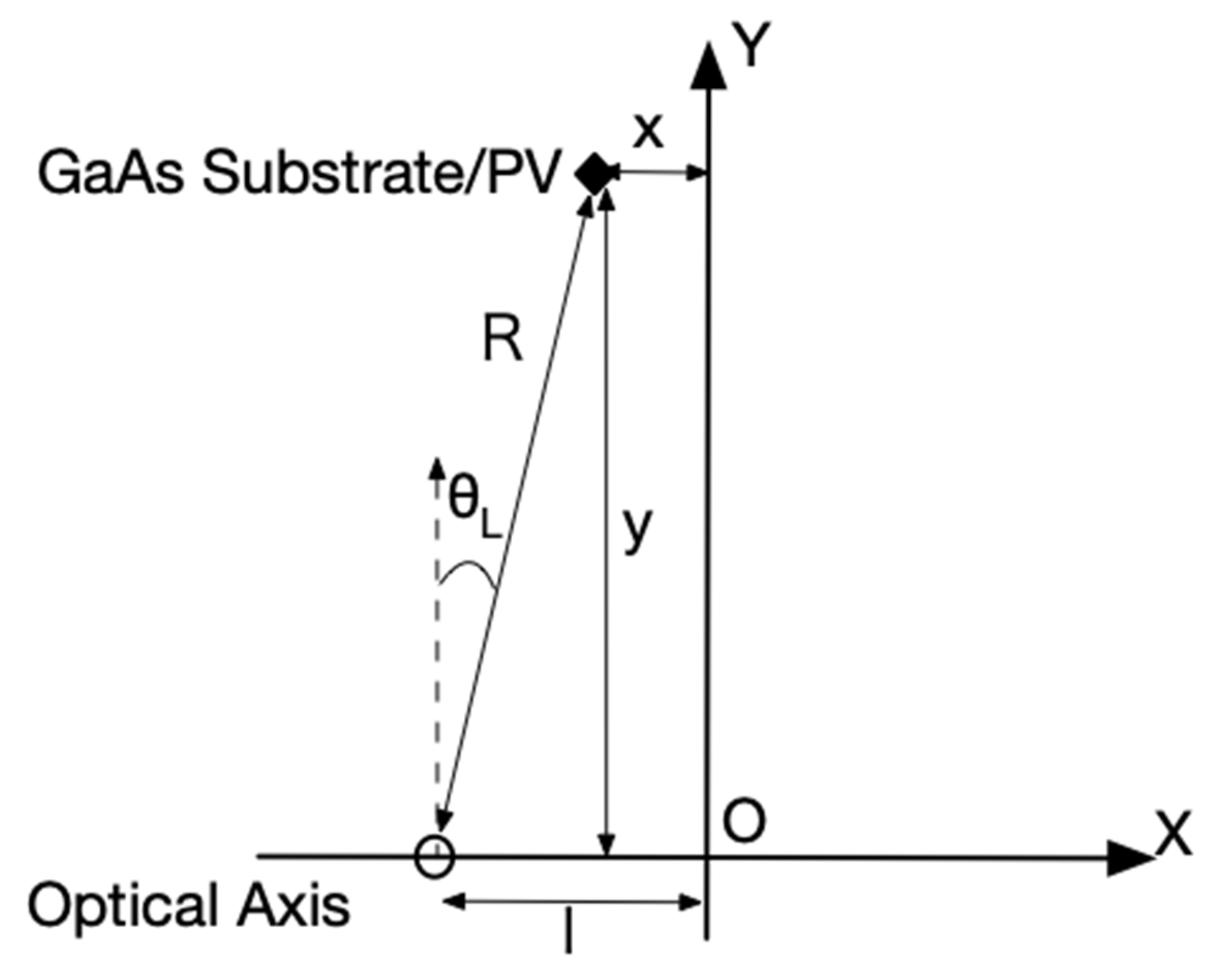
Appendix A.3. Positioning Formula without Stereo Imagery

Let R be the range from the image sensor to the target, and consider the configuration in Figure A3.
Figure A3. Configuration of positioning (mono-axis).
Photonics 10 01111 g0a3
(x, y) is obtained from the estimation of R.
x = R   s i n θ L l
y = R   c o s θ L
Like Equation (A5), θ L is calculated from pixel coordinates of the target in the pixel coordinate system. Assume that the size of the target D is known, and its apparent pixel size is P x at range R. Then, R is given by
R = D t a n θ   P x

Appendix B. Position and Direction Determination of the GaAs PV (On-Axis and Off-Axis for ϕ = 45 deg, 65 deg, 105 deg, and 125 deg)

Appendix B.1. On-Axis

Figure A4. Estimated position and direction of GaAs PV (On-axis P0). The error bars in (b) are defined by Equation (5). (a) Position. (b) Direction.
Photonics 10 01111 g0a4aPhotonics 10 01111 g0a4b
Figure A5. Estimated position and direction of the GaAs PV (On-axis P1). The error bars in (b) are defined by Equation (5). (a) Position. (b) Direction.
Photonics 10 01111 g0a5

Appendix B.2. Off-Axis

Figure A6. Position and direction determination of the GaAs PV by means of stereo imagery for ϕ   = 45 deg. The error bars in (b) are defined by Equation (5). (a) Position. (b) Direction.
Photonics 10 01111 g0a6aPhotonics 10 01111 g0a6b
Figure A7. Position and direction determination of the GaAs PV by means of stereo imagery for ϕ = 65 deg. The error bars in (b) are defined by Equation (5). (a) Position. (b) Direction.
Photonics 10 01111 g0a7
Figure A8. Position and direction determination of the GaAs PV by stereo imagery for ϕ = 105 deg. The error bars in (b) are defined by Equation (5). (a) Position. (b) Direction.
Photonics 10 01111 g0a8aPhotonics 10 01111 g0a8b
Figure A9. Position and direction determination of the GaAs PV by means of stereo imagery for ϕ = 125 deg. The error bars in (b) are defined by Equation (5). (a) Position. (b) Direction.
Photonics 10 01111 g0a9

Appendix C. Position Determination Based on Range Estimation by the Apparent Size of the Target Combined with Direction Estimation

Appendix C.1. On-Axis

Figure A10. Estimated lattice coordinate of the GaAs PV (On-axis P1). Open markers indicate the true value and solid markers are estimations.
Photonics 10 01111 g0a10
Figure A11. Estimated direction of the GaAs PV (On-axis P0, P1). The error bars are defined by Equation (5). (a) P0; (b) P1.
Photonics 10 01111 g0a11aPhotonics 10 01111 g0a11b

Appendix C.2. Off-Axis

Figure A12. Estimated position of the GaAs PV (Off-axis P0). (a) ϕ = 45 deg; (b) ϕ = 105 deg. Open markers indicate the true value and solid markers are estimations.
Photonics 10 01111 g0a12
Figure A13. Estimated direction of the GaAs PV (Off-axis P0). The error bars are defined by Equation (5). (a) ϕ = 45 deg for Position Sets 1, 2, and 3; (b) ϕ = 65 deg; (c) ϕ = 105 deg; (d) ϕ = 125 deg.
Photonics 10 01111 g0a13aPhotonics 10 01111 g0a13b

Appendix D. Position Determination with External Ranging Information

Figure A14. On-axis positioning with external ranging information. Open markers indicate the true value and solid markers are estimations. (a) P1 for Position Sets 1,2, and 3; (b) P2; (c) P3.
Photonics 10 01111 g0a14
Figure A15. Off-axis positioning with external ranging information. Open markers indicate the true value and solid markers are estimations. (a) ϕ = 45 deg for Position Set 1, 2, and 3; (b) ϕ = 65 deg; (c) ϕ = 125 deg.
Photonics 10 01111 g0a15aPhotonics 10 01111 g0a15b

References

  1. Frolova, E.; Dobroskok, N.; Morozov, A. Critical Review of Wireless Electromagnetic Power Transmission Methods. In Proceedings of the International Scientific and Practical Conference “Young Engineers of the Fuel and Energy Complex: Developing the Energy Agenda of the Future” (EAF 2021), Saint Petersburg, Russia, 10–11 December 2021; Atlantis Press: Dordrecht, The Netherlands, 2022. [Google Scholar] [CrossRef]
  2. PowerLight Technologies. Available online: https://powerlighttech.com/ (accessed on 23 May 2022).
  3. Liu, Q.; Xiong, M.; Liu, M.; Jiang, Q.; Fang, W.; Bai, Y. Charging A Smartphone Over the Air: The Resonant Beam Charging Method. IEEE Internet Things J. 2022, 9, 13876–13885. [Google Scholar] [CrossRef]
  4. The Wireless Power Company. Wi-Charge. Available online: https://www.wi-charge.com (accessed on 9 May 2022).
  5. Wang, J.X.; Zhong, M.; Wu, Z.; Guo, M.; Liang, X.; Qi, B. Ground-based investigation of a directional, flexible, and wireless concentrated solar energy transmission system. Appl. Energy 2022, 322, 119517. [Google Scholar] [CrossRef]
  6. Baraskar, A.; Yoshimura, Y.; Nagasaki, S.; Hanada, T. Space solar power satellite for the Moon and Mars mission. J. Space Saf. Eng. 2022, 9, 96–105. [Google Scholar] [CrossRef]
  7. Lee, N.; Blanchard, J.T.; Kawamura, K.; Weldon, B.; Ying, M.; Young, S.A.; Close, S. Supporting Uranus Exploration with Deployable ChipSat Probes. In Proceedings of the AIAA SCITECH 2022 Forum, San Diego, CA, USA, Virtual, 3–7 January 2022; American Institute of Aeronautics and Astronautics: Reston, VA, USA, 2022. [Google Scholar] [CrossRef]
  8. Landis, G.A. Laser Power Beaming for Lunar Polar Exploration. In Proceedings of the AIAA Propulsion and Energy 2020 Forum, Virtual Event, 24–28 August 2020; American Institute of Aeronautics and Astronautics: Reston, VA, USA, 2020. [Google Scholar] [CrossRef]
  9. Asaba, K.; Miyamoto, T. System Level Requirement Analysis of Beam Alignment and Shaping for Optical Wireless Power Transmission System by Semi–Empirical Simulation. Photonics 2022, 9, 452. [Google Scholar] [CrossRef]
  10. Asaba, K.; Miyamoto, T. Relaxation of Beam Irradiation Accuracy of Cooperative Optical Wireless Power Transmission in Terms of Fly Eye Module with Beam Confinement Mechanism. Photonics 2022, 9, 995. [Google Scholar] [CrossRef]
  11. Differential Absorption Lidar|Elsevier Enhanced Reader. Available online: https://reader.elsevier.com/reader/sd/pii/B9780123822253002048?token=ACBBE2F8761774F5628FC13C0F6B8E339140949E50BF9DE9F5063F95873CC081FB2353E862E10CA4576416252562C600&originRegion=us-east-1&originCreation=20220824035349 (accessed on 24 August 2022).
  12. Dual-Wavelength Measurements Compensate for Optical Interference|7 May 2004. Available online: https://www.biotek.com/resources/technical-notes/dual-wavelength-measurements-compensate-for-optical-interference/ (accessed on 24 August 2022).
  13. Herrlin, K.; Tillman, C.; Grätz, M.; Olsson, C.; Pettersson, H.; Svahn, G.; Wahlström, C.-G.; Svanberg, S. Contrast-enhanced radiography by differential absorption, using a laser-produced x-ray source. Investig. Radiol. 1997, 32, 306–310. [Google Scholar] [CrossRef]
  14. Asaba, K.; Moriyama, K.; Miyamoto, T. Preliminary Characterization of Robust Detection Method of Solar Cell Array for Optical Wireless Power Transmission with Differential Absorption Image Sensing. Photonics 2022, 9, 861. [Google Scholar] [CrossRef]
  15. Asaba, K.; Miyamoto, T. Solar Cell Detection and Position, Attitude Determination by Differential Absorption Imaging in Optical Wireless Power Transmission. Photonics 2023, 10, 553. [Google Scholar] [CrossRef]
  16. Lagendijk, R.; Franich, R.E.; Hendriks, E. Stereoscopic Image Processing. In Video, Speech, and Audio Signal Processing and Associated Standards; In Electrical Engineering Handbook; CRC Press: Oxford, UK, 2009; Volume 20096073, pp. 1–11. [Google Scholar] [CrossRef]
  17. Lu, Y.; Kubik, K. Stereo Image Matching Using Robust Estimation and Image Analysis Techniques for Dem Generation. In Proceedings of the International Archives of Photogrammetry and Remote Sensing. Vol. XXXIII, Part B3, Amsterdam, The Netherlands, 16–22 July 2000; The International Society for Photogrammetry and Remote Sensing: Hannover, Germany, 2000. Available online: https://www.isprs.org/proceedings/XXXIII/congress/part3/ (accessed on 11 September 2023).
  18. IKONOS Stereo Satellite Imagery, Satellite Images|Satellite Imaging Corp. Available online: https://www.satimagingcorp.com/satellite-sensors/ikonos/ikonos-stereo-satellite-images/ (accessed on 15 May 2023).
  19. “OS13CA5111A,” Opto Supply. Available online: https://www.optosupply.com/uppic/20211028118028.pdf (accessed on 29 December 2022).
  20. “OSI5FU511C-40,” Akizuki Denshi. Available online: https://akizukidenshi.com/download/OSI5FU5111C-40.pdf (accessed on 29 December 2022).
  21. “Depth Camera D435,” Intel® RealSenseTM Depth and Tracking Cameras. Available online: https://www.intelrealsense.com/depth-camera-d435/ (accessed on 15 May 2023).
  22. Intel, Intel® RealSenseTM D400 Series Data Sheet. Available online: https://www.intelrealsense.com/wp-content/uploads/2023/07/Intel-RealSense-D400-Series-Datasheet-July-2023.pdf?_ga=2.241913287.432115363.1694669790-809475082.1652760187 (accessed on 24 June 2023).
  23. “Welcome to Python.org,” Python.org. Available online: https://www.python.org/ (accessed on 24 August 2022).
  24. “Intel® RealSenseTM,” Intel® RealSenseTM Depth and Tracking Cameras. Available online: https://www.intelrealsense.com/sdk-2/ (accessed on 24 August 2022).
  25. “Open CV,” OpenCV. Available online: https://opencv.org/ (accessed on 23 August 2022).
  26. Wolfram Mathematica: Modern Technical Computing. Available online: https://www.wolfram.com/mathematica/ (accessed on 15 August 2022).
  27. Home|AXT Inc. Available online: http://www.axt.com/site/index.php?q=node/1 (accessed on 15 May 2023).
  28. 850 nm CWL, 12.5 mm Dia., Hard Coated OD 4.0 10 nm Bandpass Filter. Available online: https://www.edmundoptics.jp/p/850nm-cwl-125mm-dia-hard-coated-od-4-10nm-bandpass-filter/28574/ (accessed on 24 April 2023).
  29. 940 nm CWL, 12.5 mm Dia., Hard Coated OD 4.0 10 nm Bandpass Filter. Available online: https://www.edmundoptics.jp/p/940nm-cwl-125mm-dia-hard-coated-od-4-10nm-bandpass-filter/19778/ (accessed on 24 April 2023).
  30. ATI—Advanced Technology Institute, Inc.—BioInformatics/Mathematical Information Engineering. Available online: http://www.advanced-tech-inst.co.jp/ (accessed on 14 February 2023).
Figure 1. Layout of the experiments on position information.
Photonics 10 01111 g001
Figure 2. Procedure of generating range information from left/right differential images.
Photonics 10 01111 g002
Figure 3. Integrity measure C1.
Photonics 10 01111 g003
Figure 4. Integrity measure of Position Set 1 (GaAs substrate). (a) C1 ( ξ L ξ R ) against exposure time; (b) C2 ( η R η L ) against exposure time.
Photonics 10 01111 g004
Figure 5. Mean positioning error along Position Set 1.
Photonics 10 01111 g005
Figure 6. Estimated position of the GaAs substrate.
Photonics 10 01111 g006
Figure 7. Estimated direction of the GaAs substrate. The error bars are defined by Equation (5).
Photonics 10 01111 g007
Figure 8. Coaxial optics (external view). (a) Front view. (b) Side view.
Photonics 10 01111 g008
Figure 9. Internal configuration of the coaxial optics. (a) Left-side view. (b) Bottom view.
Photonics 10 01111 g009
Figure 10. Integrity measure of Position Sets 1, 2, and 3 (GaAs substrate). (a) C1; (b) C2.
Photonics 10 01111 g010
Figure 11. Estimated position of the GaAs substrate. (a) Position Set 1; (b) Position Set 2; (c) Position Set 3.
Photonics 10 01111 g011
Figure 12. Estimated direction of the GaAs substrate. The error bars are defined by Equation (5). (a) Position Set 1; (b) Position Set 2; (c) Position Set 3.
Photonics 10 01111 g012
Figure 13. Position estimation error of the fixed target at (0,27) (stereo imagery, with coaxial optics).
Photonics 10 01111 g013
Figure 14. Angular characteristics of center coordinates and area size determination in the pixel coordinates of the image sensor for the GaAs substrate and PV. (a) GaAs substrate; (b) GaAs PV.
Photonics 10 01111 g014
Figure 15. Position estimation error of the fixed target at (0,27) (stereo imagery, without coaxial optics). The received power in this figure is greater than Figure 13 about 8-fold. (a) Exposure Time: 50,000 μ s , 100,000 μ s , 200,000 μ s ; (b) Exposure Time: 2500 μ s , 5000 μ s , 10,000 μ s .
Photonics 10 01111 g015
Figure 16. On-axis configuration and off-axis configuration. (a) On-axis. (b) Off-axis.
Photonics 10 01111 g016
Figure 17. Estimated position and direction of the GaAs PV (on-axis P0 and P1). The error bars in (b) and (d) are defined by Equation (5). (a) Position (P0). (b) Direction (P0). (c) Position (P1). (d) Direction (P1).
Photonics 10 01111 g017
Figure 18. Estimated position and direction of the GaAs PV (off-axis P0 ϕ = 65, 125 deg). The error bars in (b) and (d) are defined by Equation (5). (a) Position (65 deg). (b) Direction (65 deg). (c) Position (125 deg). (d) Direction (125 deg).
Photonics 10 01111 g018
Figure 19. Estimated position of the GaAs substrate ( ϕ   = 110 deg).
Photonics 10 01111 g019
Figure 20. Estimated direction of the GaAs substrate ( ϕ   = 110 deg). The error bars are defined by Equation (5). (a) Position Set 1; (b) Position Set 2; (c) Position Set 3.
Photonics 10 01111 g020
Figure 21. Position estimation error of the fixed target at (0,27) (apparent target size, with coaxial optics).
Photonics 10 01111 g021
Figure 22. Position estimation error of the fixed target at (0,27) (apparent target size, without coaxial optics). The received power in this figure is greater than Figure 21 about 8-fold. (a) Exposure time = 25,000 µ s , 50,000 µ s , 100,000 µ s , 200,000 µ s . (b) Exposure time = 2500 µ s , 5000 µ s , 10,000 µ s .
Photonics 10 01111 g022
Figure 23. Estimated position of the GaAs PV. (a) On-axis P0. (b) Off-axis ϕ = 65 deg. (c) Off-axis ϕ = 125 deg.
Photonics 10 01111 g023
Figure 24. Excerpts from on-axis and off-axis position and direction estimation with external ranging information. (a) On-axis position. P0. (b) Off-axis position ( ϕ = 105 deg). P0.
Photonics 10 01111 g024
Table 1. Parameters in the experiments.
Transmitter Assembly
   LED power2 mW × 2 for λ = 850 nm and 940 nm
   Beam divergence85 deg (full angle)
   Filter paper transmittance50%/paper(typical)
Target Assembly
   GaAs substrate2-inch diameter
   GaAs PV6 cm × 4 cm
   Distance from the camera assembly660 mm(typical)
   Attitude angle43~123 deg (typical)
Camera Assembly
   CameraD435 × 2
   Exposure time25, 50, 100, 250, 500, 1000, 2500, 5000, 10,000, 25,000, 50,000, 100,000 and 200,000 μ s
   Image size640 × 480 px
Table 2. Transmittance of λ O N pass filter and λ O F F pass filter.
Transmittance   at   λ O N Transmittance   at   λ O F F
λ O N pass filter0.540
λ O F F pass filter00.27
Table 3. Comparison of the off-axis ψ between stereo imagery and apparent size measurement.
ψ R ψ ( R = 27 )
stereo imagery1 to 3 deg0.47 to 1.41
apparent size measurement2 to 5 deg9.94 to 2.35
Disclaimer/Publisher’s Note: The statements, opinions and data contained in all publications are solely those of the individual author(s) and contributor(s) and not of MDPI and/or the editor(s). MDPI and/or the editor(s) disclaim responsibility for any injury to people or property resulting from any ideas, methods, instructions or products referred to in the content.

