Full-Vectorial Light Propagation Simulation of Optimized Beams in Scattering Media

Abstract

Volumetric scattering prevents imaging modalities in biomedical optics from imaging deep inside tissue. The optimization of the incident wavefront has the potential to improve these imaging modalities. To investigate the optimization and light propagation of such beams inside scattering media rigorously, full-vectorial simulations based on solutions of Maxwell’s equations are necessary. In this publication, we present a versatile two-step beam synthesis method to efficiently simulate the scanning and phase optimization of a focused beam inside a static scattering medium. We present four different approaches to the phase optimization of the energy density and the absolute value of the Poynting vector. We find that these quantities have two regions with different, almost exponential decays over depth for a non-optimized beam. Optimization by conjugating the phase of the projected electric field in various directions at the focus shows an improvement below a certain penetration depth. Seeking global solutions to the optimization problems reveals an even better enhancement in the energy density and the absolute value of the Poynting vector in the focus. For Poynting vector optimization, the differences between the presented optimization approaches are more significant than for the energy density. With the presented method, it is possible to efficiently simulate different imaging methods improved by wavefront shaping to investigate their possible penetration depths.

1. Introduction

The scattering of light is one of the greatest obstacles preventing optical imaging modalities from imaging deep inside scattering media such as biological tissue. To reduce the amount of unwanted scattered light in the resulting image, different methods have been developed, such as confocal scanning microscopy and optical coherence tomography. Most of these techniques try to effectively reject the multiply scattered light. Therefore, this has led to the sole use of ballistic light for imaging results in the limitation of the penetration depth due to the Beer–Lambert law. Another way to reduce the scattering of light is optical clearing, which modifies the optical properties of the specimen to an almost homogeneous refractive index distribution [1]. This approach is impractical in many applications. Common approaches, which also use scattered light for imaging in the optical spectrum, such as diffuse tomography [2], have a reduced resolution compared to common microscopy techniques [3].

With the advent of spatial light modulators, the manipulation of the incident light to regain a focus inside or behind a scattering medium became possible [4,5]. Spatial light modulators are high-resolution modulators that use liquid crystal display technology, deformable mirrors, or microelectromechanical systems [6,7,8]. All of these technologies have successfully been applied to correct aberrations or focus behind a scattering medium [9,10,11]. Wavefront shaping methods have since been shown to be able to improve imaging in multiple scattering media with imaging resolutions similar to state-of-the-art microscopy techniques [12]. Frequently used methods to optimize the incident wavefront are via feedback [13], phase conjugation [14], and using the transmission matrix [15,16]. To find the optimal wavefront, one needs access to the electromagnetic field at the point of interest, which is feasible outside the scattering medium but inside the medium requires, for example, a guide star [17]. If the refractive index distribution of a specimen is known, it is theoretically possible to calculate the scattering of the incident light and optimize it via simulation.

To investigate how the electromagnetic field behaves when optimizing the incident wavefront, full-vectorial electromagnetic field simulations are an invaluable tool. Common methods to model light propagation inside diffuse media based on the radiative transfer equation are not applicable in this case because they do not describe interference effects [18]. Therefore, methods to investigate light optimization by manipulating the incident wavefront must describe interference effects. Often, these types of simulations are carried out in a waveguide geometry [19] or in two-dimensional scattering media, where only out-of-plane polarization is considered [20,21]. Other simulation approaches for wavefront shaping scenarios have used approximations of wave propagation, such as the beam propagation method [22,23].

To cover all aspects of the electromagnetic field, such as polarization and phase, full-vectorial electromagnetic field simulations based on Maxwell’s equations are needed, which is a computationally demanding task for a large medium. In this publication, we describe in Section 2 how to efficiently simulate the full-vectorial light propagation of focused beams inside static scattering media by a two-step beam synthesis method. This approach makes it possible to optimize the incident beam to enhance the energy density or the absolute value of the Poynting vector in the focus. Additionally, average values of the mentioned quantities can be obtained with our proposed method. Results for a focused beam scanned into a scattering medium and optimized via phase modulation are presented in Section 3. We conclude this study with Section 4, where we also discuss the main results.

2. Simulation Method

2.1. Two-Step Beam Synthesis Method

We use the Debye–Wolf theory [24,25] for an aplanatic optical system to simulate the scanning and optimization of a monochromatic focused beam inside a scattering static medium. A sketch of the focusing system is depicted in Figure 1. As we are interested in the simulation of a spatial light modulator in the back focal plane of the imaging system, it is convenient to model the incident beams with their angular spectrum representation.

The incident geometrical ray with an electric field ${\mathit{E}}_{\mathrm{inc}}\left(\mathit{s}\right)$ propagating parallel to the optical axis (z-axis) refracts at the Gaussian reference sphere, where $\mathit{s}=(s_x,s_y,s_z)$ denotes the normalized wavevector $\mathit{k}/k$, which is fully characterized by the two coordinates $s_x$ and $s_y$ in k-space. The wavevector is denoted by $\mathit{k}$ and the absolute value of the wavevector by $k=2\pi n_{\mathrm{m}}/\lambda$ with the vacuum wavelength $\lambda$ and the refractive index of the surrounding medium $n_{\mathrm{m}}$. For a monochromatic beam, the third component of the normalized wavevector can be calculated by $s_z={(1-s_x^2-s_y^2)}^{1/2}$. The refracted ray has an electric field ${\mathit{E}}_{\infty }\left(\mathit{s}\right)$, which is the electrical field vector of a plane wave propagating in the direction $\mathit{s}$ to the focus region. To obtain the electric field distribution $\mathit{E}\left(\mathit{r}\right)$ in the focal region, we must integrate over the whole numerical aperture, each point in k-space. This results in the representation of the focusing field with the so-called Debye–Wolf integral [24]

$$\mathit{E}\left(\mathit{r}\right)=-\frac{\mathrm{i}kf}{2\pi }{\int \int }_{s_x^2+s_y^2\le 1}{\mathit{E}}_{\infty }\left(\mathit{s}\right)exp\left(\mathrm{i}k\mathit{s}·\mathit{r}\right)\frac{1}{s_z}\mathrm{d}{s}_x\mathrm{d}{s}_y,$$

(1)

where $\mathit{r}$ denotes the position vector and f is the focal length of the imaging system. To obtain ${\mathit{E}}_{\infty }\left(\mathit{s}\right)$ from ${\mathit{E}}_{\mathrm{inc}}\left(\mathit{s}\right)$, we follow the approach presented in [26]. The incident electric field for a specific ray is decomposed into a component that is perpendicular to the meridional plane ${\mathit{E}}_{\mathrm{inc}}\left(\mathit{s}\right)·{\mathit{n}}_{\varphi }$ and a component that is parallel to the meridional plane ${\mathit{E}}_{\mathrm{inc}}\left(\mathit{s}\right)·{\mathit{n}}_{\rho }$.

The unit vector ${\mathit{n}}_{\varphi }=(-\sin \varphi ,\cos \varphi ,0)$ is perpendicular to the meridional plane and  ${\mathit{n}}_{\mathit{\rho }}=(\cos \varphi ,\sin \varphi ,0)$, the corresponding parallel unit vector. The angle $\varphi$ describes the rotation of the meridional plane around the z-axis. The electric field components are also perpendicular to the propagation direction that is parallel to the optical axis. After the geometrical ray is refracted from the Gaussian reference sphere, the propagation direction changes to $\mathit{s}$. The perpendicular part of the electric field vector remains the same after the Gaussian reference sphere but the parallel part has to change as the electric field has to be perpendicular to $\mathit{s}$. Therefore, the electric field vector for a plane wave in the angular spectrum representation can be calculated by [26]

$${\mathit{E}}_{\infty }\left(\mathit{s}\right)=\sqrt{s_z}\left[\left[{\mathit{E}}_{\mathrm{inc}}\left(\mathit{s}\right)·{\mathit{n}}_{\varphi }\right]{\mathit{n}}_{\varphi }+\left[{\mathit{E}}_{\mathrm{inc}}\left(\mathit{s}\right)·{\mathit{n}}_{\rho }\right]{\mathit{n}}_{\theta }\right].$$

(2)

The unit vector ${\mathit{n}}_{\mathit{\theta }}=(\cos \theta \cos \varphi ,\cos \theta \sin \varphi ,-\sin \theta )$ is perpendicular to the propagation direction $\mathit{s}$ and the factor $\sqrt{s_z}$ is due to energy conservation. The angle $\theta$ describes the angle between the refracted ray direction $\mathit{s}$ and the z-axis, as shown in Figure 1. We further assume that the aplanatic optical system has a polarization-independent transmission of unity. Therefore, we can write the electric field distribution at the focus with Equation (1) in terms of the angular spectrum of the incident field generated by a fully illuminated aperture as

$$\begin{array}{cc}\hfill \mathit{E}\left(\mathit{r}\right)={\int \int }_{s_x^2+s_y^2\le 1}& \left[\left[{\mathit{E}}_{\mathrm{inc}}\left(\mathit{s}\right)·{\mathit{n}}_{\varphi }\right]{\mathit{n}}_{\varphi }+\left[{\mathit{E}}_{\mathrm{inc}}\left(\mathit{s}\right)·{\mathit{n}}_{\rho }\right]{\mathit{n}}_{\theta }\right]\hfill \\ \hfill & exp\left(\mathrm{i}k\mathit{s}·\mathit{r}\right)\frac{1}{\sqrt{s_z}}\mathrm{d}{s}_x\mathrm{d}{s}_y,\hfill \end{array}$$

(3)

where we omit the constant factors outside the integral.

For a given incident field distribution in k-space, Equation (3) can be calculated numerically to obtain the field distribution around the focus in free space. The incident field to the focus region can be used as the input for a numerical Maxwell’s equations solver, such as the FDTD method [27], to calculate the scattering of a beam incident on a turbid medium. Scanning the incident beam to many positions relative to the scattering medium is computationally expensive as Maxwell’s equations have to be solved for each position. In this study, we use a two-step beam synthesis method, which we already have applied for beam propagation in two-dimensional scattering media [21]. We first discretize the double integral in Equation (3) with a sum over equidistant points in k-space

$$\begin{array}{cc}\hfill \mathit{E}\left(\mathit{r}\right)\approx \sum _{\mathrm{i}}\sum _{\mathrm{j}}& \left[\left[{\mathit{E}}_{\mathrm{inc},\mathrm{i},\mathrm{j}}·{\mathit{n}}_{\varphi }\right]{\mathit{n}}_{\varphi }+\left[{\mathit{E}}_{\mathrm{inc},\mathrm{i},\mathrm{j}}·{\mathit{n}}_{\rho }\right]{\mathit{n}}_{\theta }\right]\hfill \\ \hfill & exp\left(\mathrm{i}k{\mathit{s}}_{\mathrm{i},\mathrm{j}}·\mathit{r}\right)\frac{1}{\sqrt{s_{z,\mathrm{i},\mathrm{j}}}}\mathsf{\Delta }{s}_x\mathsf{\Delta }{s}_y,\hfill \end{array}$$

(4)

where $\mathsf{\Delta }{s}_x$ and $\mathsf{\Delta }{s}_y$ denote the spacing between the equidistant points in k-space. Each term in the sum corresponds to a plane wave propagating in the direction ${\mathit{s}}_{\mathrm{i},\mathrm{j}}$ to the focus region with a polarization vector calculated by Equation (2). For a given scattering medium, Maxwell’s equations are solved for each plane wave with ${\mathit{s}}_{\mathrm{i},\mathrm{j}}$, which results in a set of N near-field solutions. In this publication, we are interested in monochromatic beams that are scattered by a dielectric medium. Therefore, we solve Maxwell’s equations on a grid with a modified Born series approach similar to the one described in [28]. Because we only examine phase modulation in this study, we restrict ourselves to incident fields with the polarization ${\mathit{E}}_{\mathrm{inc}}=(E_0,0,0)$ and constant amplitude $E_0$ in the back focal plane. The calculation of the set of N near fields is the most time-consuming part, where the bottleneck is a single plane wave simulation. Discretization of the double integral in Equation (3) leads to the repetition of the fields in the x- and y-planes. To avoid aliasing, we have to consider the Whittaker–Shannon sampling theorem [29]. Therefore, the spacing between neighboring k-vectors has to be

$$\mathsf{\Delta }{s}_i\le \frac{2\pi }{L_{i}k},i\in \{x,y\},$$

(5)

where $L_i$ is the lateral height and width of the simulation region.

In the second step of the two-step beam synthesis method, all N near fields are added according to the angular spectrum in k-space to numerically approximate the integral in Equation (3). Thus, the plane wave part in Equation (4) is replaced by the field distribution over the simulation grid ${\mathit{E}}_{\mathrm{i},\mathrm{j}}\left(\mathit{r}\right)$ to obtain the scattered electric field distribution inside the medium

$$\mathit{E}\left(\mathit{r}\right)\approx \sum _{\mathrm{i}}\sum _{\mathrm{j}}{\mathit{E}}_{\mathrm{i},\mathrm{j}}\left(\mathit{r}\right)\frac{1}{\sqrt{s_{z,\mathrm{i},\mathrm{j}}}}\mathsf{\Delta }{s}_x\mathsf{\Delta }{s}_y.$$

(6)

The summation is also done for the magnetic field distribution and results in the corresponding total magnetic field $\mathit{H}\left(\mathit{r}\right)$ due to the linearity of Maxwell’s equations. The magnetic field has to be computed in order to calculate the energy density distribution $w\left(\mathit{r}\right)$ and the complex Poynting vector $\mathit{S}\left(\mathit{r}\right)$ inside the medium.

Scanning the incident beam by $\mathsf{\Delta }\mathit{r}$ only requires a phase shift for each plane wave in the angular spectrum of $exp\left(-\mathrm{i}k\mathit{s}·\mathsf{\Delta }\mathit{r}\right)$. Therefore, the term $exp\left(-\mathrm{i}k{\mathit{s}}_{\mathit{i},\mathit{j}}·\mathsf{\Delta }\mathit{r}\right)$ needs to be added in Equation (6) under the double sum. In addition, the angular spectrum can also be altered to optimize the focused incident beam to increase the energy density or the Poynting vector at a specific position. In this publication, we consider only phase modulation in the angular spectrum, although polarization and amplitude modulation are also possible with this method. For each optimization channel, a phase factor of $exp(-\mathrm{i}{\varphi }_{opti,i,k})$ can be applied to spatially modulate the phase of the incident beam in the back focal plane. There are different ways to optimize a certain observable, such as the energy density or the Poynting vector, with the knowledge of the electromagnetic field distribution from the plane wave set but, in general, this is a global optimization problem.

2.2. Phase Optimization Techniques

The optimization of the incident electromagnetic field to obtain, for example, a focus inside a scattering medium requires either a feedback signal [13] or information about the electromagnetic field [30] at the region of interest. The total number of optimization channels $N_{\mathrm{ch}}$ is usually given by the experiment setup. Often, a spatial light modulator is used, where each pixel or a group of pixels equals one optimization channel. In a full-vectorial light simulation, it is possible to access the electromagnetic field anywhere in the simulation region. Therefore, the information for optimization is easily accessible. In general, the incident light can be optimized for any objective function. Here, we focus on the energy density $w\left(\mathit{r}\right)$ and the absolute value of the Poynting vector $|\Re (\mathit{S}\left(\mathit{r}\right)\left)\right|$. $\Re \left(\right)$ denotes the real part. The energy density is calculated as $w\left(\mathit{r}\right)=\frac{1}{4}(ϵ\left(\mathit{r}\right)\mathit{E}\left(\mathit{r}\right)·{\mathit{E}}^{*}\left(\mathit{r}\right)+{\mu }_0\mathit{H}\left(\mathit{r}\right)·{\mathit{H}}^{*}\left(\mathit{r}\right))$ and the complex Poynting vector as $\mathit{S}\left(\mathit{r}\right)=\frac{1}{2}\mathit{E}\left(\mathit{r}\right)\times {\mathit{H}}^{*}\left(\mathit{r}\right)$. Each channel has an electromagnetic field denoted by ${\tilde{\mathit{E}}}_n\left(\mathit{r}\right)$, ${\tilde{\mathit{H}}}_n\left(\mathit{r}\right)$, which can be calculated by summing up the electromagnetic fields ${\mathit{E}}_{\mathrm{i},\mathrm{j}}\left(\mathit{r}\right)$ and ${\mathit{H}}_{\mathrm{i},\mathrm{j}}\left(\mathit{r}\right)$ over the corresponding region of the n-th channel in k-space.

One of the most common attempts to optimize the energy density or intensity of the electromagnetic field inside or behind a scattering medium is to use phase conjugation. This technique results in the maximum constructive interference of the electric fields, but only if light can be modeled as a scalar or all incident channels have the same polarization state in the focus position. For phase conjugation, looking only at the x component of the electric field ${\tilde{E}}_{n,\mathrm{x}}\left({\mathit{r}}_{\mathrm{foc}}\right)$ at the optimization position ${\mathit{r}}_{\mathrm{foc}}$, we apply a phase change of $exp(-\mathrm{i}arg\left\{{\tilde{E}}_{n,\mathrm{x}}\left({\mathit{r}}_{\mathrm{foc}}\right)\right\})$ to each channel. This phase shift is also applied to the magnetic fields. The energy density and the Poynting vector are then calculated with these fields and are further denoted by “x-pc”.

Scattering randomizes the phase and polarization state of light for each channel. Thus, it can be expected that phase conjugation with respect to a random direction ${\mathit{n}}_{\mathrm{rand}}$ inside strongly scattering media can also enhance the energy density or absolute value of the Poynting vector. Phase conjugation along a random direction is obtained by projecting the electric field at ${\mathit{r}}_{\mathrm{foc}}$ of each optimization channel along ${\mathit{n}}_{\mathrm{rand}}$ and applying this phase shift of $exp\left(-\mathrm{i}arg\left\{{\tilde{\mathit{E}}}_{\mathrm{n}}\left({\mathit{r}}_{\mathrm{foc}}\right)·{\mathit{n}}_{\mathrm{rand}}\right\}\right)$ to the electromagnetic field of each channel. We further denote the optimized quantities obtained by this method as “n-rand-pc”.

It is known that the electric field vector can only oscillate in a plane [31], even inside a strongly scattering medium. Therefore, the optimized electric field vector oscillates also in a plane. One option to optimize the incident field is to find the best direction ${\mathit{n}}_{\mathrm{opti}}(\varphi ,\theta )=\left(\cos \varphi \sin \theta ,\sin \varphi \sin \theta ,\cos \theta \right)$ in which to project the electric fields of each channel to find the optimal phase shift. To find the optimal direction, we must solve the following optimization problem for the energy density $w_{\mathrm{foc}}={〈w〉}_t\left({\mathit{r}}_{\mathrm{foc}}\right)$ at the focus ${\mathit{r}}_{\mathrm{foc}}$

$$\begin{array}{cccc}\hfill & \underset{\varphi ,\theta }{\mathrm{maximize}}\hfill & \hfill & {\left|\sum _{n=1}^{N_{\mathrm{ch}}}{\tilde{\mathit{E}}}_n\left({\mathit{r}}_{\mathrm{foc}}\right)e^{-\mathrm{i}arg\left\{{\mathit{n}}_{\mathrm{opti}}(\varphi ,\theta )·{\tilde{\mathit{E}}}_n\left({\mathit{r}}_{\mathrm{foc}}\right)\right\}}\right|}^2+{\left|\sum _{n=1}^{N_{\mathrm{ch}}}{\tilde{\mathit{H}}}_n\left({\mathit{r}}_{\mathrm{foc}}\right)e^{-\mathrm{i}arg\left\{{\mathit{n}}_{\mathrm{opti}}(\varphi ,\theta )·{\tilde{\mathit{E}}}_n\left({\mathit{r}}_{\mathrm{foc}}\right)\right\}}\right|}^2\hfill \\ \hfill & \mathrm{subject}\mathrm{to}\hfill & \hfill & 0<\varphi \le 2\pi ,\hfill \\ \hfill & \hfill & & 0<\theta \le \pi .\hfill \end{array}$$

(7)

Here, it should be noted that we are using the electric field to project along the optimal direction ${\mathit{n}}_{\mathrm{opti}}$ to find the optimal angles for $\varphi$ and $\theta$. This could also be done with the magnetic field. In the same way, we can write the optimization problem for the average value of the Poynting vector $\Re \left(\mathit{S}\left({\mathit{r}}_{\mathrm{foc}}\right)\right)$ as

$$\begin{array}{cccc}\hfill & \underset{\varphi ,\theta }{\mathrm{maximize}}\hfill & \hfill & \Re \left[\left(\sum _{n=1}^{N_{\mathrm{ch}}}{\tilde{\mathit{E}}}_n\left({\mathit{r}}_{\mathrm{foc}}\right)e^{-\mathrm{i}arg\left\{{\mathit{n}}_{\mathrm{opti}}(\varphi ,\theta )·{\tilde{\mathit{E}}}_n\left({\mathit{r}}_{\mathrm{foc}}\right)\right\}}\right)\times \left(\sum _{n=1}^{N_{\mathrm{ch}}}{\tilde{\mathit{H}}}_n^{*}\left({\mathit{r}}_{\mathrm{foc}}\right)e^{\mathrm{i}arg\left\{{\mathit{n}}_{\mathrm{opti}}(\varphi ,\theta )·{\tilde{\mathit{E}}}_n\left({\mathit{r}}_{\mathrm{foc}}\right)\right\}}\right)\right]\hfill \\ \hfill & \mathrm{subject}\mathrm{to}\hfill & \hfill & 0<\varphi \le 2\pi ,\hfill \\ \hfill & \hfill & & 0<\theta \le \pi .\hfill \end{array}$$

(8)

Solving Equations (7) and (8) involves only the variables $\varphi$ and $\theta$. We further denote this optimization scheme as “n-opti”.

The maximal number of variables that can be optimized is the number of channels $N_{\mathrm{ch}}$ if each channel can be phase modulated. Therefore, the optimization problem for the energy density in the focus point can be written as

$$\begin{array}{cccc}\hfill & \underset{\varphi ,\theta }{\mathrm{maximize}}\hfill & \hfill & {\left|\sum _{n=1}^{N_{\mathrm{ch}}}{\tilde{\mathit{E}}}_n\left({\mathit{r}}_{\mathrm{foc}}\right)e^{-\mathrm{i}\mathsf{\Delta }{\varphi }_n}\right|}^2+{\left|\sum _{n=1}^{N_{\mathrm{ch}}}{\tilde{\mathit{H}}}_n\left({\mathit{r}}_{\mathrm{foc}}\right)e^{-\mathrm{i}\mathsf{\Delta }{\varphi }_n}\right|}^2\hfill \\ \hfill & \mathrm{subject}\mathrm{to}\hfill & \hfill & 0<\mathsf{\Delta }{\varphi }_n\le 2\pi ,n=1,2,3...N_{\mathrm{ch}}.\hfill \end{array}$$

(9)

Furthermore, the optimization problem for the average value of the Poynting vector in the focus position is

$$\begin{array}{cccc}\hfill & \underset{\varphi ,\theta }{\mathrm{maximize}}\hfill & \hfill & \left[\left(\sum _{n=1}^{N_{\mathrm{ch}}}{\tilde{\mathit{E}}}_n\left({\mathit{r}}_{\mathrm{foc}}\right)e^{-\mathrm{i}\mathsf{\Delta }{\varphi }_n}\right)\times \left(\sum _{n=1}^{N_{\mathrm{ch}}}{\tilde{\mathit{H}}}_n^{*}\left({\mathit{r}}_{\mathrm{foc}}\right)e^{\mathrm{i}\mathsf{\Delta }{\varphi }_n}\right)\right]\hfill \\ \hfill & \mathrm{subject}\mathrm{to}\hfill & \hfill & 0<\mathsf{\Delta }{\varphi }_i\le 2\pi ,n=1,2,3...N_{\mathrm{ch}}.\hfill \end{array}$$

(10)

In further sections, we denote quantities optimized with all the possible $N_{\mathrm{ch}}$ channels as “g-opti”. To find optimal solutions for Equations (7)–(10), we use the Julia packages Optim.jl [32] and Blackboxoptim.jl [33].

2.3. Scattering Medium and System Specifications

In Figure 2, the turbid medium that is used in this study is shown. The scattering medium is built up by cubic scatterers randomly positioned in a host medium with refractive index $n_{\mathrm{m}}=1$. We choose to use cubic scatterers with the same orientation because it is easy to randomly position them without overlapping with a large concentration. Each cubic scatterer has a side length of $0.7\lambda$ and a real refractive index of 1.5. Hence, the medium is non-absorbing. The scatterers are randomly distributed inside a rectangular volume with side lengths $L_x=41.7\lambda$, $L_y=41.7\lambda$, and $L_z=20\lambda$. The volume fraction occupied inside the rectangular volume is $f_{\mathrm{V}}=0.3$. The concentration and refractive index of the scatterers were determined by test simulations in such a way that the medium scatters relatively strongly. This medium is similar, for example, to a thin powder layer of silica particles of similar size and concentration. The refractive index distribution of the randomly positioned cubic scatterer was transferred into a simulation grid that had a resolution of $\lambda /6$.

To quantify the scattering mean free path ℓ of the turbid medium, we performed a simulation, where a plane wave was scattered by the turbid medium. The propagation of the plane wave was in the z-direction and we applied periodic boundary conditions in the x- and y-direction to avoid artifacts from the finite size of the medium. Furthermore, the polarization of the incident plane wave was in the x-direction. The coherent intensity, which is often defined as ${〈E_x〉}_{x,y}^2\left(z\right)$, can be used as an estimator for ℓ [35]. The averaging of $E_x\left(\mathit{r}\right)$ was performed over the x- and y-direction of the simulation volume. The normalized coherent intensity ${〈E_x〉}_{x,y}^2\left(z\right)/{〈E_0〉}^2$ is shown in Figure 2b, where ${〈E_0〉}^2$ is the absolute square of the amplitude of the incident plane wave. A different approach to obtaining an estimate of ℓ is to mimic a collimated transmission experiment by performing the plane wave simulation, as described before, for different widths $L_z$ of the medium. Calculating the two-dimensional Fourier transform of $E_x$ at a transverse plane behind the medium gives the far field. The normalized intensity from the collimated transmission simulations is shown with orange markers in Figure 2b. Both approaches give similar estimates of the coherent (unscattered) intensity. A fit of an exponential function gives a scattering mean free path of $\ell =1.05\lambda$. The scattering mean free path is often estimated with the scattering efficiency of a single scatterer and the concentration of the scatterers [36]. If we assume a medium with the spherical scatterers but the same volume as a single scatterer, as in this study, we find that this approach would give an estimation of $\ell =0.62\lambda$, which is a ≈$40$ relative difference from the numerical approaches. A concentration of $f_{\mathrm{V}}=0.1$ would give a relative difference of ≈$4.6$ between the different approaches. It is known that this linear dependency between the inverse of the scattering mean free path and scatterer concentration is only valid for small concentrations. Therefore, we used the decay of the coherent intensity and the collimated transmission simulations to estimate the scattering mean free path.

The simulated incident focused beam is defined by the imaging system described in the previous section. In this study, we choose a numerical aperture of $\mathrm{NA}=0.45$, which results in a maximum angle of ${\theta }_{\max }=26.74{}^{°}$ relative to the optical axis for the allowed k-vectors. The numerical aperture limits the area in k-space as depicted in Figure 1. In order to use the two-step beam synthesis method, we have to simulate each k-vector in a separate simulation; therefore, we have to sample the aperture. We choose an equidistant spacing of $\mathsf{\Delta }{s}_x=\mathsf{\Delta }{s}_y=0.025$ according to Equation (5) to avoid artifacts coming from the repetition of the incident beams in the lateral direction. The sampling of the aperture in normalized k-space is shown in Figure 3.

In total, we simulated $N=1009$ plane waves for the uniform illumination of the back focal plane and polarization of ${\mathit{E}}_{\mathrm{inc}}=(E_0,0,0)$.

3. Results

The described vectorial two-step beam synthesis method is capable of simulating the scanning and optimization of arbitrary electromagnetic beams inside turbid media. In this section, we present results obtained with this simulation approach to scan inside a scattering medium and visualize the energy density distribution and the absolute value of the Poynting vector. Afterward, we investigate the impact of phase optimization for different numbers of optimization channels for these quantities.

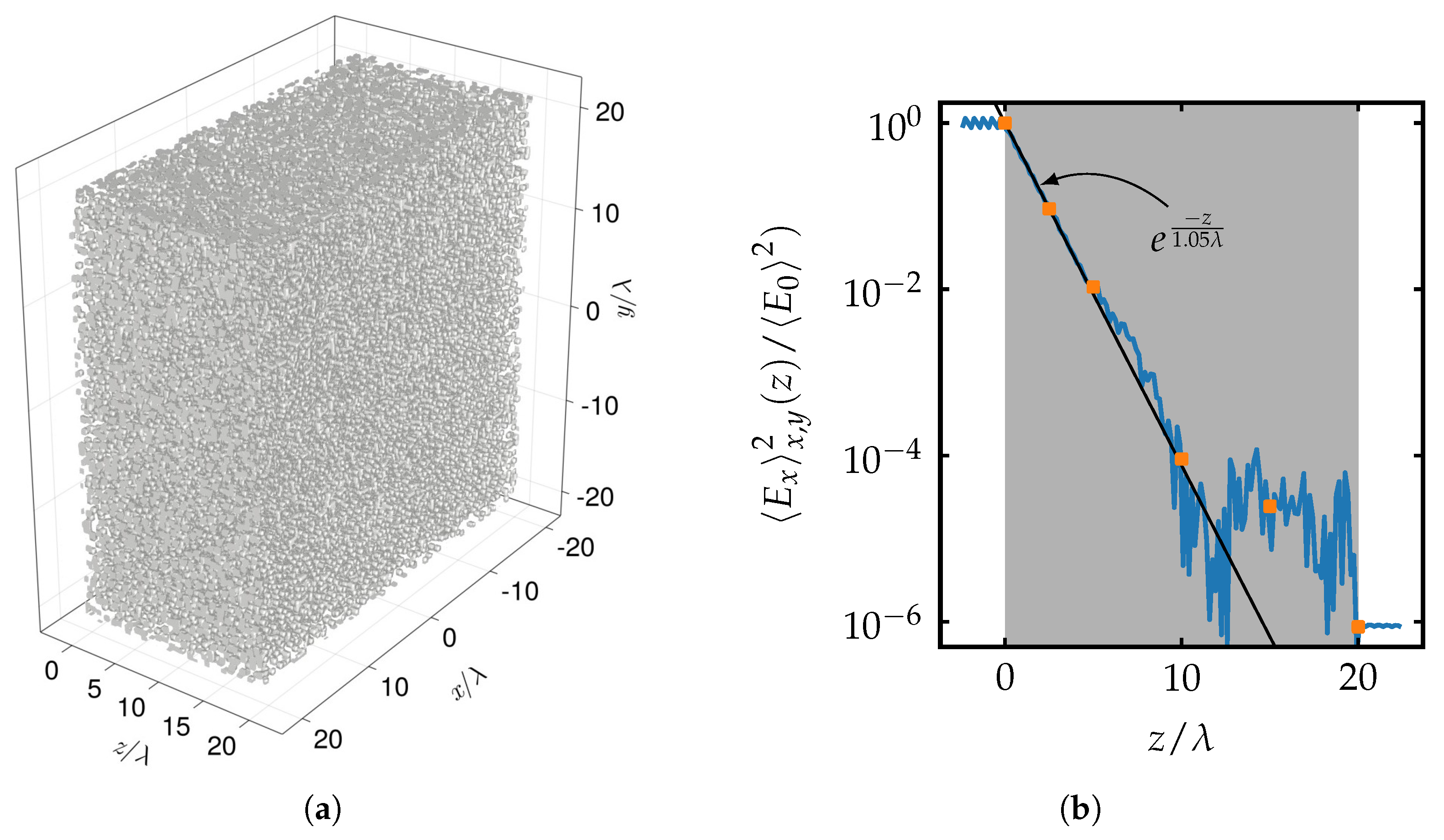
3.1. Scattering of a Focused Beam by the Turbid Medium

Scanning a focused beam into a scattering medium results in the redistribution of the incident light. If the scattering mean free path ℓ is much smaller than the scanning depth, the focus completely deteriorates, which makes the focused beam unusable for imaging modalities such as confocal microscopy. To illustrate the scattering of a focused beam inside a highly scattering slab, we scanned the focus to a depth of $z=15\lambda$ inside the scattering medium. The normalized energy density distribution of the beam in vacuum $w\left(\mathit{r}\right)/w_0$ is shown in Figure 4a. A clear focus at the position ${\mathit{r}}_{\mathrm{foc}}=(0,0,15\lambda )$ with $w\left(\mathit{r}\right)/w_0=1$ can be seen. $w_0$ denotes the energy density at the focus position in vacuum. The full width at half maximum of the focus in vacuum is ≈$8.5\lambda$ in the axial direction and ≈$1.1\lambda$ in the lateral direction. Scanning the focused beam to the same position in the presence of the scattering medium results in the energy density distribution shown in Figure 4b. The effect of scattering reduces the energy density inside the medium because a lower amount of light enters the scattering medium and also the energy is distributed over a larger volume. The maximum normalized energy density inside the scattering medium is $0.35$ and its location is about a distance of $\lambda$ from the entrance surface. At the original focus, the energy density drops by around two orders of magnitude to $w\left({\mathit{r}}_{\mathrm{foc}}\right)/w_0=0.003$.

In the same way, the Poynting vector can be investigated. In Figure 5a, the absolute value of the Poynting vector is shown, which is normalized by the peak value in vacuum at the focus position further denoted by $\left|\Re \left({\mathit{S}}_0\right)\right|$. The largest value can be found in the focus as expected. The full width at half maximum of the focus for $\left|\Re \left({\mathit{S}}_{\mathrm{foc}}\left(\mathit{r}\right)\right)\right|/\left|\Re \left({\mathit{S}}_0\right)\right|$ is ≈$8.5\lambda$ in the axial direction and ≈$1.1\lambda$ in the lateral direction. These are the same values as for the focus size of the energy density. Introducing the scattering medium leads to the redirection of the flow of light, as can be seen in Figure 5b. Furthermore, a reduction in the intensity of the Poynting vector is additionally caused by the backscattered light, which leads to a counterpropagating flow of light, reducing the overall Poynting vector.

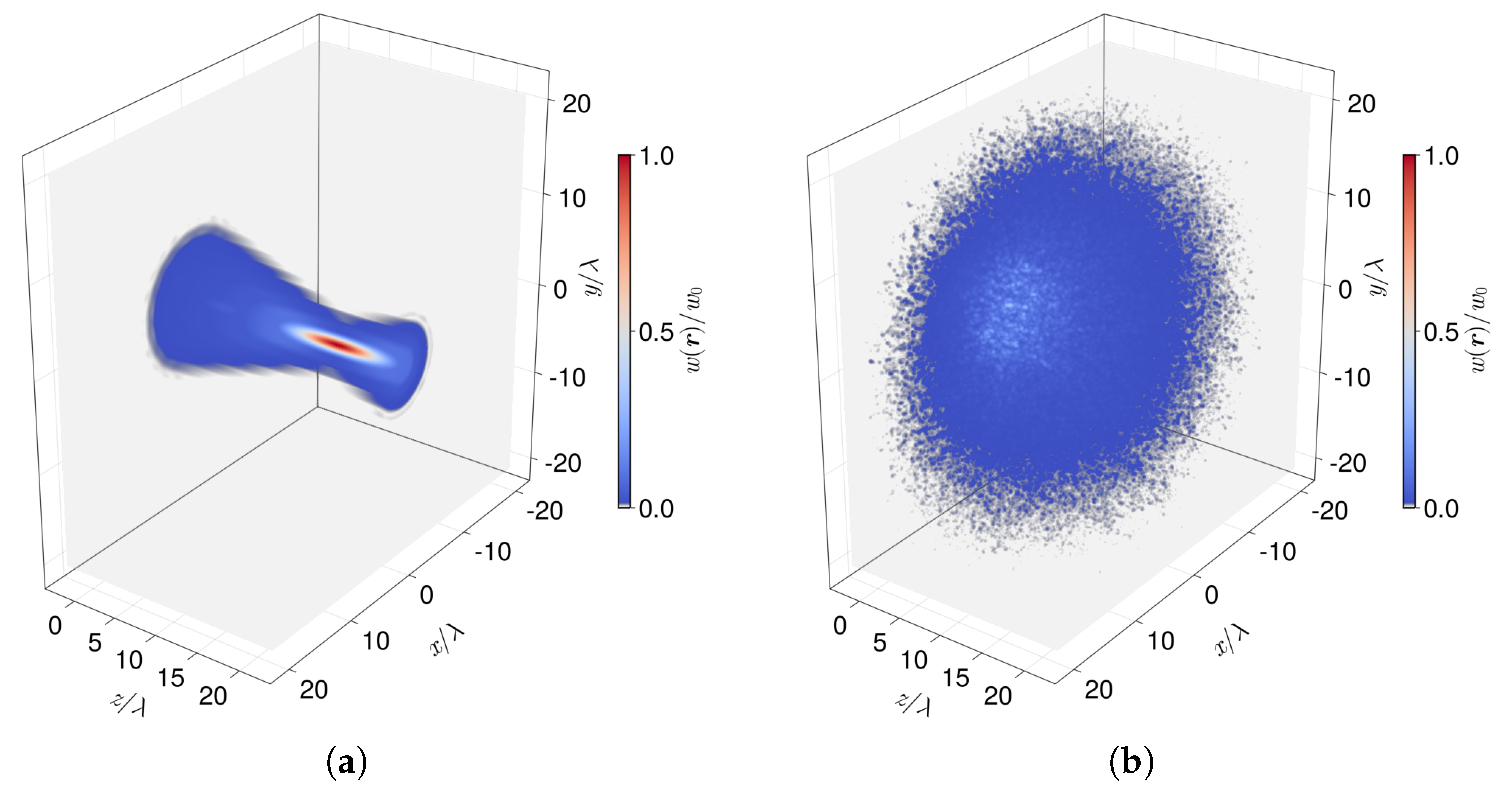
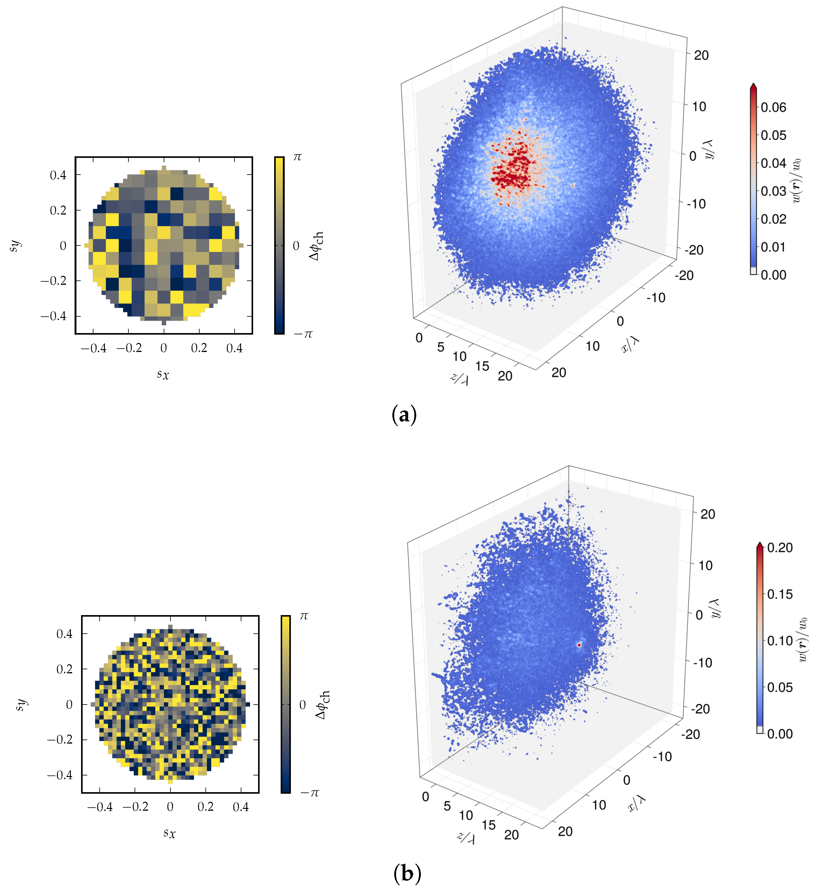
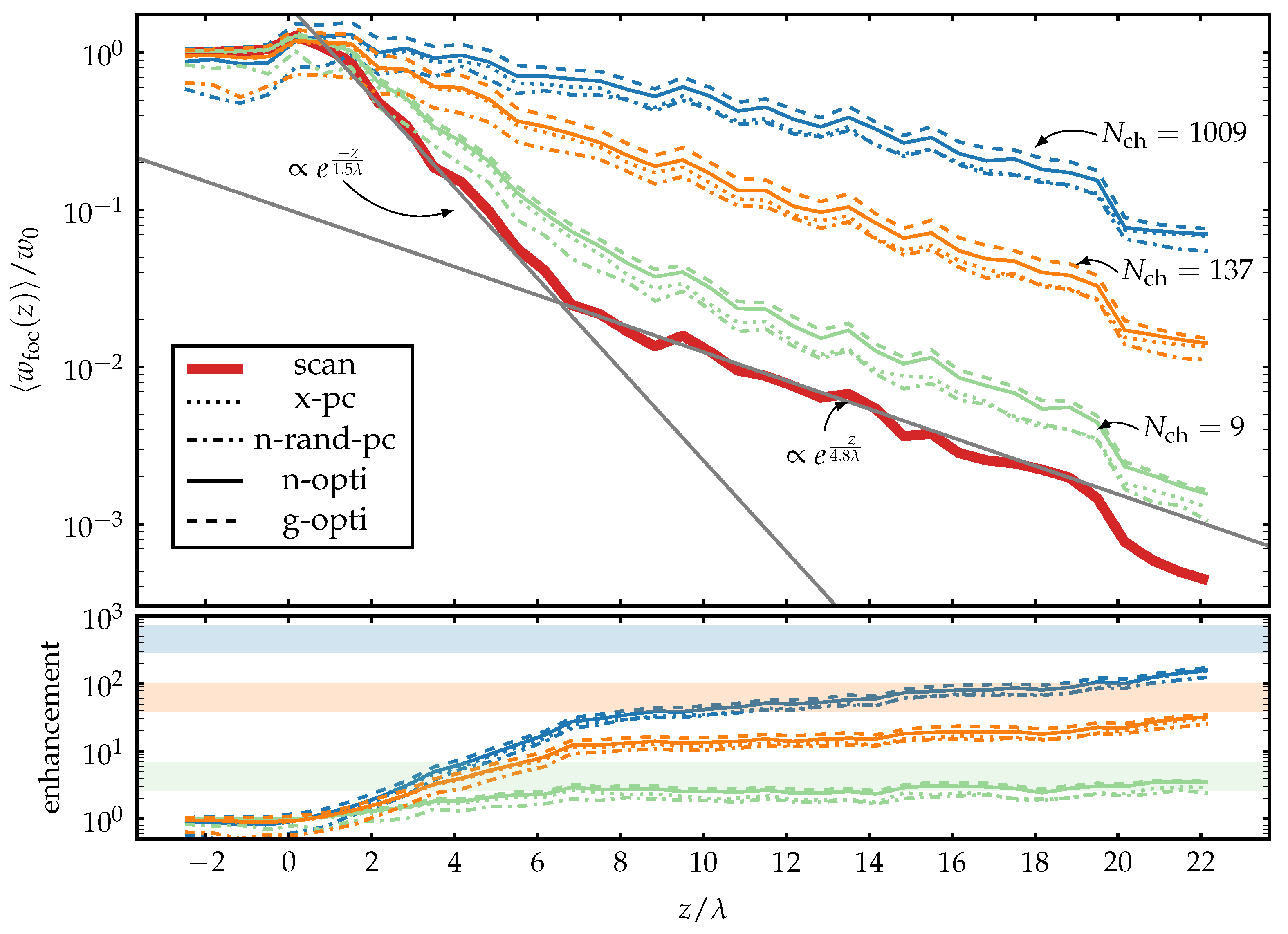
3.2. Phase Optimization to Enhance the Focus Energy Density

By scanning a focused beam into a scattering medium, the focus inevitably deteriorates, as shown in the previous Section 3.1. Phase optimization can lead to an increase in the energy density at the desired focus location.

In Figure 6, two simulations of phase-optimized beams are shown. The non-optimized focused light beams were first scanned to a depth of $z=15\lambda$ and afterward optimized with $N_{\mathrm{ch}}=137$ (Figure 6a) and $N_{\mathrm{ch}}=1009$ (Figure 6b) equally sized channels. Equally sized channels refer to the channels with the largest rectangular area in k-space that is modulated. There are additional channels with smaller areas at the edge of the circular region in k-space that are modulated, but we do not count them here as full optimization channels. For these examples, an optimal solution according to Equation (9) was sought. The phase distributions applied in k-space are shown in the left plots and the resulting energy density distribution of the optimized incident beams are shown in the right plots.

After phase optimization with $N_{\mathrm{ch}}=137$, a distinct speckle-sized focus is regained at $z=15\lambda$. It can also be noticed that in the volume close to the incident surface, the energy density has a larger value as in the desired focus. Optimization with $N_{\mathrm{ch}}=1009$ results also in a speckle-sized focus but with a greater value of the energy density in the focus than in any other region of the scattering medium. The reason for this is that as the number of channels increases, the electromagnetic fields constructively interfere only in the focus, and, in other regions, the field results in a random interference pattern. The axial and lateral full width at half maximum of the focus is ≈$0.6\lambda$ for $N_{\mathrm{ch}}=137$ and $N_{\mathrm{ch}}=1009$.

To obtain the quantitative behavior of the energy density in the focus, we scanned the non-optimized and optimized beams into the medium to obtain the energy density in the focus over depth. Different optimization schemes and different numbers of optimization channels were used to obtain an enhancement in the energy density in the focus. Here, we define the enhancement as the quotient of the optimized and the non-optimized quantity. The non-optimized quantity is denoted by “scan”. In Figure 7 (top), the averaged energy density $〈w_{\mathrm{foc}}\left(z\right)〉$ over depth normalized by the energy density in the focus in vacuum $w_0$ for non-optimized (“scan”) and optimized (“x-pc”, “n-rand-pc”, “n-opti”, and “g-opti”) beams is shown. The results from the optimized beams are shown with different line styles and the colors denote the different numbers of optimization channels. The averaging was performed over 49 lateral positions between the area of $-6\lambda$ and $6\lambda$ in the x and y-direction, where each lateral position was separated by at least a distance of $2\lambda$. By using only a small limited lateral area, we aimed to avoid boundary effects due to the finite size of the medium. The enhancement over depth is shown in Figure 7 (bottom). The shaded areas show the expected enhancement, where the maximum value for a specific $N_{\mathrm{ch}}$ is obtained by the scalar theory [4] from the formula $\eta \left(N_{\mathrm{ch}}\right)=\pi /4(N_{\mathrm{ch}}-1)+1$. The minimum value is obtained by $\eta \left(N_{\mathrm{ch}}\right)/3$. This can be justified by the consideration that the polarization of a general electromagnetic field has three spatial degrees of freedom and these orthogonal polarization states cannot interfere.

For the scanned non-optimized beam, the normalized energy density in the focus first increases for shallow depths up to a distance $2\lambda$ inside the medium. This can be explained by the backscattered light from larger depths enhancing the focus energy density on average. For depths $z>2\lambda$, $〈w_{\mathrm{foc}}\left(z\right)〉/w_0$ decreases exponentially with a factor ≈$1/1.5\lambda$, which is lower than predicted by the Beer–Lambert law. This deviation can be explained due to the presence of scattered light in the focus. The behavior of the energy density changes for depths larger than $10\lambda$ to an exponential decay with ≈$1/4.8\lambda$. This phenomenon is also present in two-dimensional, strongly scattering media [21]. Behind the medium, $〈w_{\mathrm{foc}}\left(z\right)〉/w_0$ drops abruptly due to the absence of backscattered light from larger depths.

In Figure 7 (top), we see that applying the conjugate phase of the electric field of each channel at the focus in the x-direction (“x-pc”) or a random direction (“n-rand-pc”) leads to no enhancement or even a decrease in the energy density in the focus for depths up to $2\lambda$. As the electric field of the incident beam is predominantly polarized in the x-direction, conjugating the phase in this direction leads to almost no enhancement before the scattering medium and at shallow depths because all the electromagnetic fields of the channels are already in phase at the focus. For larger depths, modulating the incident beam with the two different phase conjugation approaches leads also to a significant enhancement. The results of the approaches “n-opti” and “g-opti”, which utilize global optimization algorithms to find an optimal solution of the phase patterns, show similar behavior before the scattering medium and at shallow depths with a small or no enhancement compared to the non-optimized beam. For larger depths, the enhancement is always greater for these types of optimization approaches. Furthermore, optimization according to the “g-opti” approach gives always a greater energy density in the focus than “n-opti”, but one has to keep in mind that “g-opti” uses $N_{\mathrm{ch}}$ variables in the optimization problems, whereas “n-opti” only uses two. The enhancement with all optimization approaches shows a steep increase until a depth of $z=8\lambda$. This effect can be explained by the fact that the focused incident beam is itself optimized for a vacuum and deteriorates when scanned into the scattering medium. After a depth of $z>8\lambda$, the focus is practically lost, and therefore the enhancements for different numbers of incident channels stagnate or have a decreased slope. For the energy density enhancement, only the results for $N_{\mathrm{ch}}=9$ reach the theoretically expected enhancement between $\eta \left(9\right)/3=2.4$ and $\eta \left(9\right)=7.3$. For more optimization channels, the different electromagnetic fields might not be completely randomized for the scanned non-optimized beam and the consulted scalar theory might not be fully applicable to vectorial light propagation.

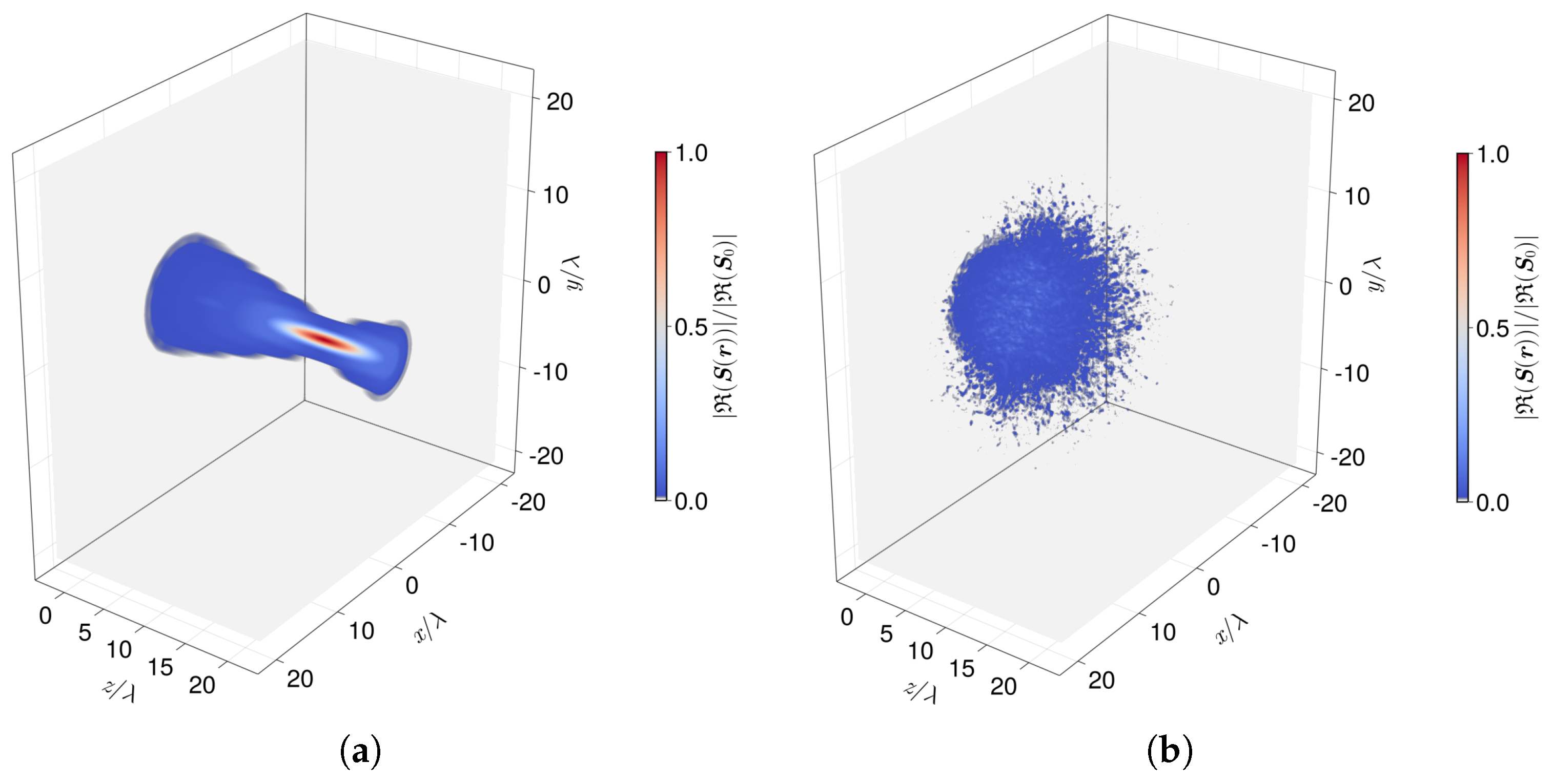
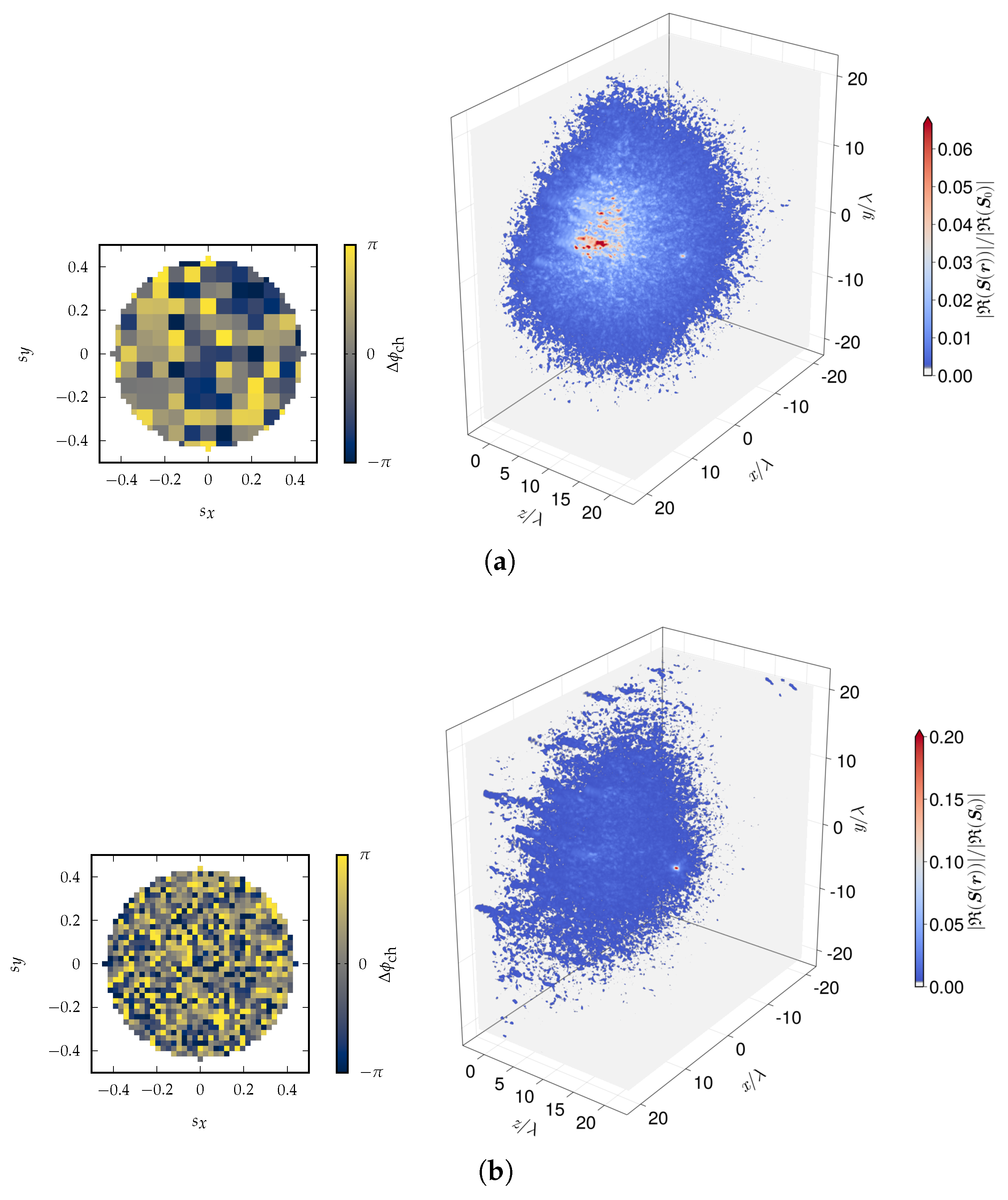
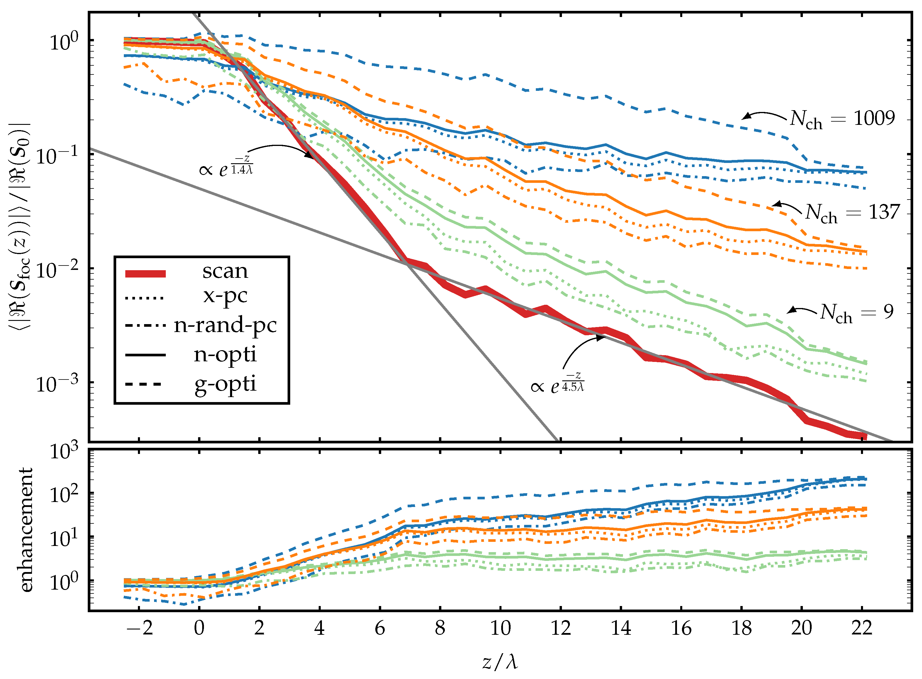
3.3. Phase Optimization to Enhance the Absolute Value of the Focus Poynting Vector

In addition, it is often of interest to investigate the flow of light described by the Poynting vector and how it can be increased by the phase modulation of the incident beam. As seen in Figure 5, a scattering medium reduces the absolute value of the Poynting vector in the focus compared to the value in vacuum ${\mathit{S}}_0$. Phase optimization according to Equation (10) enhances the absolute value of the Poynting vector at the desired focus. This can be seen for a scanning position at $z=15\lambda$ in Figure 8 for two different numbers of optimization channels. We find that in the case of $N_{\mathrm{ch}}=137$, a distinct focus is regained at the desired focus position, although $\left|\Re \left(\mathit{S}\left({\mathit{r}}_{\mathrm{foc}}\right)\right)\right|/\left|\Re \left({\mathit{S}}_0)\right)\right|$ can have greater values in the scattering medium at shallow depths. For $N_{\mathrm{ch}}=1009$, the maximum absolute value of the Poynting vector is in the desired focus and also larger as for the simulation with $N_{\mathrm{ch}}=137$. In both cases, the full width at half maximum in the lateral direction is ≈$0.7\lambda$ and in the axial direction ≈$0.3\lambda$.

Examining the average absolute value of the Poynting vector for a non-optimized beam over the scanning depth shows a decrease with penetration depth, as can be seen in Figure 9. Averaging was performed in the same way as for the energy density. Furthermore, the absolute value of the Poynting vector does not show an increase in value at shallow depths compared to the energy density in the previous section. This can be explained by the counter-propagating waves from the scattering medium, which lead to a resulting average decrease in the Poynting vector. We also find two regions within the medium with different exponential decays, at first with an exponential of ≈$1/1.4\lambda$ until $z=8\lambda$ and with ≈$1/4.5\lambda$ until the end of the medium. Both exponential behaviors have a slightly lower decay rate compared to the Beer–Lambert law.

Phase optimization to enhance the absolute value of the Poynting vector has been done for three different numbers of optimization channels $N_{\mathrm{ch}}\in \left\{9,137,1009\right\}$. The four different optimization approaches described in Section 2.2 were used for optimization. The results are shown in Figure 9 in different colors and line styles. For scanning positions in front of the medium, all optimization techniques besides “g-opti” deteriorate the focus compared to the non-optimized beam and result in a lower value of $〈\left|\Re \left({\mathit{S}}_{\mathrm{foc}}\left(z\right)\right)\right|〉/\left|\Re \left({\mathit{S}}_0\right)\right|$. For a scanning depth greater than $4\lambda$, all optimization techniques lead to an increase in the absolute value of the Poynting vector in the focus. At scanning positions inside the medium, we find that the differences between the global optimization technique “g-opti” and the other approaches increase with an increase in the number of optimization channels. Behind the medium, the “n-opti” and “g-opti” approaches lead to similar values of the average absolute value of the Poynting vector in the focus. The enhancement with the different techniques increases with the scanning depth for all approaches and is shown in Figure 9 in the bottom plot.

4. Discussion and Conclusions

In this study, we extended the two-step beam synthesis approach already used to investigate light propagation and optimization in two-dimensional media [21,37] to be able to model full-vectorial light propagation and optimization in three dimensions. The presented method is split into two main steps. First, a set of plane wave near-field solutions for a static medium is obtained by numerically solving Maxwell’s equations, where the incident polarization and the propagation direction of the plane waves are determined through the Debye–Wolf theory. In the second step, the near fields of arbitrary incident beams scattered by the medium can be computed by adding the plane wave near-field solutions according to the angular spectrum of the incident beam. The separation of the calculation of the plane wave solutions and the synthesis of a complex beam makes it possible to reuse the plane wave solutions. Thus, with this method, the scattering of different incident beams can be efficiently calculated for the static medium under consideration. This includes scanning and optimizing the incident beam. Common methods would have to perform the complete numerical calculation again for each change in the incident beam.

We used this approach to simulate the scanning and phase optimization of a focused beam with a numerical aperture of $\mathrm{NA}=0.45$ inside a strongly scattering medium with a scattering mean free path of $\ell =1.05\lambda$ and thickness $20\lambda$. We examined the energy density and absolute value of the Poynting vector at the intended focus position over depth ranging from $-2.5\lambda$ to $22\lambda$, where $0\lambda$ was the location of the front surface of the scattering medium. The optimization of the incident beam was investigated for a different number of optimization channels $N_{\mathrm{ch}}\in \left\{9,137,1009\right\}$ and different optimization schemes. To find an optimal phase pattern to regain a focus, we used the knowledge of the electromagnetic field at the intended focus position. The energy density and the absolute value of the Poynting vector in the focus showed two regions over depth, with first a steep and afterward a flatter, exponential-like decay. This can also be found in two-dimensional scattering media [21] but is not present in thin media or scattering media with a larger ℓ. For example, the absence of the two regions can be found in simulations for a scattering medium with $\ell =1.95\lambda$ (not presented in this publication) and two-dimensional media [38]. Phase optimization by modulating the phase in k-space and applying the conjugate phase of the electric field in x or a random direction in the focus for each optimization channel can lead to a significant enhancement inside the scattering medium. An increased enhancement can be obtained by seeking a solution to the optimization problem to find the best direction in which to project the electric field to obtain the phase for phase conjugation. This requires two optimization variables. The best performance was always achieved when a solution for the “g-opti” was sought, but with the drawback that the $N_{\mathrm{ch}}$ variables have to be optimized for the given objective function. An additional drawback of the presented simulation approach is that one near-field simulation takes around 30 min, and, for a larger volume and a larger numerical aperture, the number of required near-field solutions increases drastically. However, with increasing computing power and a larger number of parallel simulations, this approach can be accelerated.

The versatility of the presented method makes it possible to model arbitrary vectorial light beams. Possible applications of the approach are the investigation of different electromagnetic quantities inside turbid media, as shown in this study for the energy density and the Poynting vector. This can be of importance to quantify the performance of imaging modalities. Another possible use case is the calculation of optimal phase patterns computationally for real turbid media with a measured refractive index distribution to improve imaging modalities [23]. For large turbid media, the numerical solutions of Maxwell’s equations are often too time-consuming to obtain. Therefore, it is also possible to use our proposed method but with plane wave solutions obtained with approximations such as the beam propagation method.

References

1. Zhu, D.; Larin, K.V.; Luo, Q.; Tuchin, V.V. Recent progress in tissue optical clearing. Laser Photonics Rev. 2013, 7, 732–757. [Google Scholar] [CrossRef]
2. Durduran, T.; Choe, R.; Baker, W.B.; Yodh, A.G. Diffuse optics for tissue monitoring and tomography. Rep. Prog. Phys. 2010, 73, 076701. [Google Scholar] [CrossRef] [PubMed]
3. Gigan, S. Optical microscopy aims deep. Nat. Photonics 2017, 11, 14–16. [Google Scholar] [CrossRef]
4. Vellekoop, I.M.; Mosk, A. Focusing coherent light through opaque strongly scattering media. Opt. Lett. 2007, 32, 2309–2311. [Google Scholar] [CrossRef] [PubMed]
5. Mosk, A.P.; Lagendijk, A.; Lerosey, G.; Fink, M. Controlling waves in space and time for imaging and focusing in complex media. Nat. Photonics 2012, 6, 283–292. [Google Scholar] [CrossRef]
6. Maurer, C.; Jesacher, A.; Bernet, S.; Ritsch-Marte, M. What spatial light modulators can do for optical microscopy. Laser Photonics Rev. 2011, 5, 81–101. [Google Scholar] [CrossRef]
7. Bifano, T. MEMS deformable mirrors. Nat. Photonics 2011, 5, 21–23. [Google Scholar] [CrossRef]
8. Ren, Y.X.; Lu, R.D.; Gong, L. Tailoring light with a digital micromirror device. Ann. Der Phys. 2015, 527, 447–470. [Google Scholar] [CrossRef]
9. Kubby, J.; Gigan, S.; Cui, M. Wavefront Shaping for Biomedical Imaging; Cambridge University Press: Cambridge, UK, 2019. [Google Scholar]
10. Galaktionov, I.; Nikitin, A.; Samarkin, V.; Sheldakova, J.; Kudryashov, A.V. Laser beam focusing through the scattering medium-low order aberration correction approach. In Proceedings of the Unconventional and Indirect Imaging, Image Reconstruction, and Wavefront Sensing 2018, San Diego, CA, USA, 22–23 August 2018; Volume 10772, pp. 259–272. [Google Scholar]
11. Paudel, H.P.; Stockbridge, C.; Mertz, J.; Bifano, T. Focusing polychromatic light through scattering media. In Mems Adaptive Optics VII; SPIE: Bellingham, WA, USA, 2013; Volume 8617, pp. 82–88. [Google Scholar]
12. Gigan, S.; Katz, O.; De Aguiar, H.B.; Andresen, E.R.; Aubry, A.; Bertolotti, J.; Bossy, E.; Bouchet, D.; Brake, J.; Brasselet, S.; et al. Roadmap on wavefront shaping and deep imaging in complex media. J. Phys. Photonics 2022, 4, 042501. [Google Scholar] [CrossRef]
13. Vellekoop, I.M. Feedback-based wavefront shaping. Opt. Express 2015, 23, 12189–12206. [Google Scholar] [CrossRef]
14. Yaqoob, Z.; Psaltis, D.; Feld, M.S.; Yang, C. Optical phase conjugation for turbidity suppression in biological samples. Nat. Photonics 2008, 2, 110–115. [Google Scholar] [CrossRef]
15. Yoon, J.; Lee, K.; Park, J.; Park, Y. Measuring optical transmission matrices by wavefront shaping. Opt. Express 2015, 23, 10158–10167. [Google Scholar] [CrossRef] [PubMed]
16. Popoff, S.; Lerosey, G.; Fink, M.; Boccara, A.C.; Gigan, S. Image transmission through an opaque material. Nat. Commun. 2010, 1, 81. [Google Scholar] [CrossRef] [PubMed]
17. Horstmeyer, R.; Ruan, H.; Yang, C. Guidestar-assisted wavefront-shaping methods for focusing light into biological tissue. Nat. Photonics 2015, 9, 563–571. [Google Scholar] [CrossRef] [PubMed]
18. Martelli, F.; Tiziano, B.; Del Bianco, S.; André, L.; Alwin, K. Light Propagation Through Biological Tissue and Other Diffusive Media: Theory, Solutions, and Validations; SPIE: Bellingham, WA, USA, 2022. [Google Scholar]
19. Bender, N.; Yamilov, A.; Goetschy, A.; Yılmaz, H.; Hsu, C.W.; Cao, H. Depth-targeted energy delivery deep inside scattering media. Nat. Phys. 2022, 18, 309–315. [Google Scholar] [CrossRef]
20. Tseng, S.H.; Yang, C. 2-D PSTD Simulation of optical phase conjugation for turbidity suppression. Opt. Express 2007, 15, 16005–16016. [Google Scholar] [CrossRef] [PubMed]
21. Ott, F.; Fritzsche, N.; Kienle, A. Numerical simulation of phase-optimized light beams in two-dimensional scattering media. JOSA A 2022, 39, 2410–2421. [Google Scholar] [CrossRef] [PubMed]
22. Yang, J.; Li, J.; He, S.; Wang, L.V. Angular-spectrum modeling of focusing light inside scattering media by optical phase conjugation. Optica 2019, 6, 250–256. [Google Scholar] [CrossRef]
23. Thendiyammal, A.; Osnabrugge, G.; Knop, T.; Vellekoop, I.M. Model-based wavefront shaping microscopy. Opt. Lett. 2020, 45, 5101–5104. [Google Scholar] [CrossRef]
24. Wolf, E. Electromagnetic diffraction in optical systems-I. An integral representation of the image field. Proc. R. Soc. Lond. Ser. A Math. Phys. Sci. 1959, 253, 349–357. [Google Scholar]
25. Richards, B.; Wolf, E. Electromagnetic diffraction in optical systems, II. Structure of the image field in an aplanatic system. Proc. R. Soc. Lond. Ser. A Math. Phys. Sci. 1959, 253, 358–379. [Google Scholar]
26. Novotny, L.; Hecht, B. Principles of Nano-Optics; Cambridge University Press: Cambridge, UK, 2012. [Google Scholar]
27. Çapoğlu, İ.R.; Taflove, A.; Backman, V. Computation of tightly-focused laser beams in the FDTD method. Opt. Express 2013, 21, 87–101. [Google Scholar] [CrossRef] [PubMed]
28. Krüger, B.; Brenner, T.; Kienle, A. Solution of the inhomogeneous Maxwell’s equations using a Born series. Opt. Express 2017, 25, 25165–25182. [Google Scholar] [CrossRef] [PubMed]
29. Goodman, J.W. Introduction to Fourier Optics; Roberts and Company Publishers: Englewood, CO, USA, 2005. [Google Scholar]
30. Popoff, S.M.; Lerosey, G.; Carminati, R.; Fink, M.; Boccara, A.C.; Gigan, S. Measuring the transmission matrix in optics: An approach to the study and control of light propagation in disordered media. Phys. Rev. Lett. 2010, 104, 100601. [Google Scholar] [CrossRef] [PubMed]
31. Born, M.; Wolf, E. Principles of Optics: Electromagnetic Theory of Propagation, Interference and Diffraction of Light; Elsevier: Amsterdam, The Netherlands, 2013. [Google Scholar]
32. Mogensen, P.K.; Riseth, A.N. Optim: A mathematical optimization package for Julia. J. Open Source Softw. 2018, 3, 615. [Google Scholar] [CrossRef]
33. BlackBoxOptim.jl. Available online: https://web.archive.org/web/20230326084433/https://github.com/robertfeldt/BlackBoxOptim.jl (accessed on 29 May 2023).
34. Danisch, S.; Krumbiegel, J. Makie.jl: Flexible high-performance data visualization for Julia. J. Open Source Softw. 2021, 6, 3349. [Google Scholar] [CrossRef]
35. Ishimaru, A. Wave Propagation and Scattering in Random Media; Academic Press: New York, NY, USA, 1978; Volume 2. [Google Scholar]
36. Bohren, C.F.; Huffman, D.R. Absorption and Scattering of Light by Small Particles; John Wiley & Sons: Hoboken, NJ, USA, 2008. [Google Scholar]
37. Elmaklizi, A.; Schäfer, J.; Kienle, A. Simulating the scanning of a focused beam through scattering media using a numerical solution of Maxwell’s equations. J. Biomed. Opt. 2014, 19, 071404. [Google Scholar]
38. Elmaklizi, A.; Reitzle, D.; Brandes, A.; Kienle, A. Penetration depth of focused beams in highly scattering media investigated with a numerical solution of Maxwell’s equations in two dimensions. J. Biomed. Opt. 2015, 20, 065007. [Google Scholar] [CrossRef]
Figure 1. Illustration of the focusing system with the optical axis along the z direction. The incident light is characterized in k-space by the normalized coordinates  s x  and  s y  with its angular spectrum  E inc ( s ) . The in- and out-of-plane polarizations of  E inc ( s )  with respect to the meridional plane (plane rotated by  ϕ  around the optical axis) can be calculated with the normal vectors  n ϕ  and  n ρ . The aplanatic lens refracts the incident light at the Gaussian reference sphere. The resulting electric field vector  E ( s )  for the plane wave propagating in direction  s  is calculated with the normal vectors  n ϕ  and  n θ . The refracted light then propagates with angle  θ  relative to the optical axis to the focus region.
Photonics 10 01068 g001
Figure 2. (a) Scattering medium composed of cubic scatterers (this plot and all subsequent three-dimensional plots were produced with Makie [34]) with  f V = 0.3  and normalized dimensions  L x = 41.7 λ L y = 41.7 λ , and  L z = 20 λ . The x-, y-, and z-axis are normalized by the wavelength  λ . (b) Determination of by the decay of the coherent intensity (blue line) and collimated transmission simulations (orange markers). The black line shows the obtained exponential law with  = 1.05 λ  and the gray shaded area shows the region of the medium.
Photonics 10 01068 g002
Figure 3. Equidistant distribution of the 1009 sampling points over the numerical aperture with NA = 0.45 (gray region).
Photonics 10 01068 g003
Figure 4. Energy density distribution of a beam focused at  z = 15 λ . Panel (a) shows  w ( r ) / w 0  of the focused beam in vacuum and panel (b) when the scattering medium is present. The color for energy density values  < 0.01  is made transparent for better visibility.
Photonics 10 01068 g004
Figure 5. The absolute value of the Poynting vector of a beam focused at  z = 15 λ . Panel (a) shows  ( S foc ( r ) ) / ( S 0 )  of the focused beam in vacuum and panel (b) when the scattering medium is present. For values  < 0.01 , the color is transparent for better visibility.
Photonics 10 01068 g005
Figure 6. Energy density distribution of phase-optimized beams at  z = 15 λ . Panel (a) shows the optimized phase pattern depicted in the left plot for 137 optimization channels and the resulting normalized energy density distribution  w ( r ) / w 0  after applying the optimized phase pattern. Panel (b) shows the optimized phase pattern depicted in the left plot for 1009 optimization channels and  w ( r ) / w 0  after applying the optimized phase pattern in the right plot. Values of  w ( r ) / w 0 < 0.003  (a) and < 0.008  (b) are transparent for better visibility.
Photonics 10 01068 g006
Figure 7. (Top): Average focus energy density for the non-optimized beam scanned over depth z and phase-optimized beams obtained for different optimization methods (line style) and with different numbers of optimization channels (colors). The gray lines depict exponential decays. (Bottom): Enhancement between the scanned and phase-optimized average energy density in the focus over depth. The shaded areas show the interval between the expected enhancement from the scalar theory and one third of it.
Photonics 10 01068 g007
Figure 8. Distribution of the absolute values of the Poynting vector of phase-optimized beams at  z = 15 λ . Panel (a) shows the optimized phase pattern depicted in the left plot for 137 optimization channels and the resulting  S ( r foc ) / S 0 )  after applying the optimized phase pattern. Panel (b) shows the optimized phase pattern depicted in the left plot for 1009 optimization channels and the resulting  S ( r foc ) / S 0 )  after applying the optimized phase pattern. The applied phase shifts are shown in the inset. Values of the normalized absolute value of the Poynting vector <0.002 (a) and < 0.004  (b) are transparent for better visibility.
Photonics 10 01068 g008
Figure 9. Top plot: Average absolute value of the Poynting vector in the focus for the non-optimized beam scanned over depth z and phase-optimized beams obtained for different optimization methods (linestyle) and with different numbers of optimization channels (colors). The gray lines depict exponential decays. Bottom plot: Enhancement between the scanned and phase-optimized average absolute value of the Poynting vector in the focus over depth.
Photonics 10 01068 g009
Disclaimer/Publisher’s Note: The statements, opinions and data contained in all publications are solely those of the individual author(s) and contributor(s) and not of MDPI and/or the editor(s). MDPI and/or the editor(s) disclaim responsibility for any injury to people or property resulting from any ideas, methods, instructions or products referred to in the content.