Polarimetric Images of Biological Tissues Based on the Arrow Decomposition of Mueller Matrices

Abstract

Polarimetric techniques are widely used in a vast number of applications such as remote sensing, material characterization, astronomy and biological tissue inspection. In this last scenario, different polarimetric observables have proved their potential for enhancing imaging visualization. In this work we use a set of polarimetric observables derived from the arrow decomposition of the Mueller matrix for the first time: enpolarizing, retarding and depolarizing descriptors. In particular, the mean intensity coefficient and the three indices of polarimetric purity, the absolute values and Poincaré orientations of diattenuation, polarizance, entrance retardance and exit retardance vectors are considered. Results show images with enhanced visualization or even revealing invisible structures when compared to standard intensity images. In particular, thanks to these metrics, we improve the visualization of the necrotic areas of a Vitis rupestris leaf. In the case of animal samples, boundaries between different fascicles inside a tendon of an ex vivo chicken sample are revealed, as is the directionality of fiber tracts of the subcortical white matter in an ex vivo cow brain. The experimental results show the potential for biophotonics imaging and how polarimetric techniques could be useful for biomedical and botanical applications.

1. Introduction

Mueller polarimetry constitutes a powerful tool to generate images of a material sample based on the spatial variation of polarization descriptors derived from the corresponding point-to-point Mueller matrices (M). Even though the sixteen elements of a given Mueller matrix can be used to build their respective images, each of those elements are related in an intricate manner to the polarimetric properties of the sample at the particular point under consideration. Consequently, the identification of appropriate sets of physical parameters representing, in a separate manner, the fundamental (phenomenological) polarimetric properties of the sample at each point, appears a key aspect to optimize the contrast in imaging polarimetry, while the said properties can be monitored and represented.

From this point of view, in the specialized literature, there is a wide number of polarimetric observables derived from M that allow a physical interpretation of some characteristics of samples [1,2,3,4,5,6]. In particular, one can mention properties such as [2]:

• diattenuation and polarizance vectors, which can be obtained from the first row and column of M, respectively [7,8];
• depolarization, which can be globally characterized by means of the depolarization index (or degree of polarimetric purity) [7], the polarization entropy [9], the depolarization power [8], the first and second Lorentz depolarization indices [10], the overall purity index [11], etc., while the detailed information on depolarization can be characterized by the indices of polarimetric purity [12,13];
• retardance, whose characterization for general Mueller matrices requires a criterion to define both the entrance and exit retardance vectors.

A number of these observables have also proved their suitability in terms of biological tissue imaging and characterization [14,15,16,17,18,19]. This is because most biological samples show spatially heterogeneous polarimetric responses depending on the particular tissues they are composed of. In this sense, some works provide the relation of some physiological characteristics of tissues to polarimetric signals. For instance, Danijela et al., in the work [20], relate the anisotropy in collagen fibers by connecting them to birefringent values, to different cancer stages in tumors of epithelial origin.

Additionally, in references [21,22], the anisotropy levels and the orientation disorder are directly related to heart pathologies such as infarction. Therefore, in these cases, both the birefringent and depolarizing properties can help to differentiate between these different (healthy and pathological) kinds of tissue.

Moreover, structures such as collagen, with a high presence in animal tissue, and cellulose, present in vegetal tissue, are highly birefringent structures [23,24,25]. Depolarizing responses are also related to multiple scattering due to the high presence of scattering centers in tissues [26,27]. Dichroism carries information about the absorption of light in tissue structures depending on the polarization of light. In the case of plant samples, this helps in the detection of the organization and concentration of chloroplasts and related organelles in plant species [28]. In [29], the authors provide a list of animal and human samples where different tissue regions and pathologies were inspected by means of imaging polarimetry.

As a consequence of the above, in the last few years, the use of polarimetric imaging has been broadly used in the field of biomedicine [14,30,31,32,33,34,35,36,37,38,39,40] and plant studies [41,42,43,44,45,46], for instance, to study heart capillary structures in myocardium tissue [14,36], the visualization of brain fiber tracks [47,48], the presence of raphides in plants [42], classification of different kinds of tissue [31,36], cancerous tissues inspection in cancerous prostate [30,49], colon [32,33], skin [50], and plant pathologies [15], among others [51,52,53,54,55].

As previously discussed, a particular spatial physiological modification is connected to a specific polarimetric change. Note that if these different responses are produced in different spatial regions of the sample, we will obtain better visualization (enhanced contrast) through polarimetric imaging. In this framework, this work focuses on studying the suitability of a different set of observables, derived from the so-called arrow decomposition of Mueller matrices [56], in biological applications. To this aim, the Mueller matrix of a given sample at a given point is entered into the arrow decomposition, which allows for the decoupling of sixteen meaningful and significant independent polarimetric properties. Note that other well-known serial decompositions of Mueller matrices do not provide such a decoupling; in particular, the Lu–Chipman decomposition [8] contains a depolarizer that also involves both polarizance and retardance [57], while the normal form decomposition contains equivalent diattenuators whose diattenuation and polarizance do not match those of the sample as a whole [58]. Furthermore, the indices of polarimetric purity [12] (describing the depolarizing properties of the material sample) of the depolarizers associated with both indicated approaches are in general different from those of the original Mueller matrix [2].

In this work, the arrow decomposition approach is applied to the obtainment of sets of sixteen images for a series of biological tissue samples (two of animal origin, and one of vegetal origin), leading to improved contrast with respect to other conventional approaches. The results obtained are discussed and analyzed from both a physical and a physiological point of view.

The contents of this communication are organized as follows. Section 2 contains a summary of the concepts and notations that are necessary to formulate and analyze the new polarimetric imaging approach. Section 3 is devoted to describing a set of polarimetric observables derived from the arrow decomposition. Afterwards, in Section 4, materials and methods are provided. In Section 5, we show the polarimetric images of three different biological samples (Vitis rupestris leaf, tendinous tissue from a chicken leg and a coronal section of a cow brain), and they are compared to standard intensity images to highlight the visualization improvement associated with arrow-decomposition-based observables. Finally, Section 6 provides the main conclusions of the work.

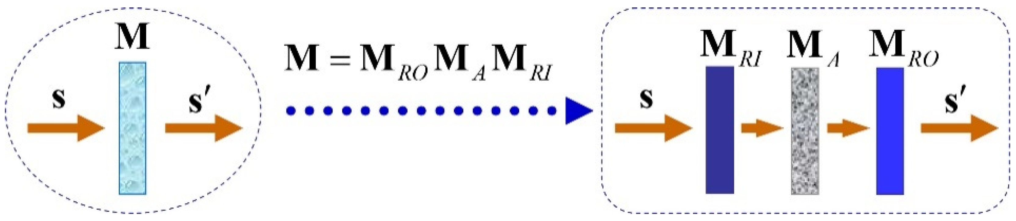
2. Theoretical Background

Linear polarimetric interactions are characterized by means of their corresponding Mueller matrices, which encompass all the measurable information regarding the changes of the Stokes parameters of the polarized light probe for each given interaction condition (angle of incidence and spectral profile of light, angle of observation, spot-size of the sample, measurement time, etc.).

Let us consider the transformation of polarized light by the action of a linear medium (under fixed interaction conditions). It can always be formulated as $s^{\prime }=Ms$ where s and $s^{\prime }$ are the Stokes vectors that represent the states of polarization of the incident and emerging light beams, respectively, while M is the Mueller matrix associated with this kind of interaction and can always be expressed as [8,59,60].

$$\begin{array}{c}M=m_{00}\widehat{M},\hspace{0.17em}\hspace{0.17em}\hspace{0.17em}\hspace{0.17em}\widehat{M}\equiv \left(\begin{array}{cc}1& D^T\\ P& m\end{array}\right),\\ m\equiv \frac{1}{m_{00}}\left(\begin{array}{ccc}{m}_{11}& m_{12}& m_{13}\\ m_{21}& m_{22}& m_{23}\\ m_{31}& m_{32}& m_{33}\end{array}\right),\\ D\equiv \frac{{\left(m_{01},m_{02},m_{03}\right)}^T}{m_{00}},\hspace{0.17em}\hspace{0.17em}P\equiv \frac{{\left(m_{10},m_{20},m_{30}\right)}^T}{m_{00}},\end{array}$$

(1)

where $m_{ij}$ $(i,j=0,1,2,3)$ are the elements of M; the superscript T indicates transpose matrix; $m_{00}$ is the mean intensity coefficient (MIC), i.e., the ratio between the intensity of the emerging light and the intensity of incident unpolarized light; D and P are the diattenuation and polarizance vectors, with absolute values D (diattenuation) and P (polarizance); and m is the normalized 3 × 3 submatrix associated with M.

Leaving aside systems exhibiting magneto-optic effects, given a Mueller matrix M, the Mueller matrix that represents the same linear interaction as M, but with the incident and emergent directions of the propagation of the electromagnetic wave interchanged, is given by [2,61,62]

$$M^r=\mathrm{diag}\left(1,1,-1,1\right)\hspace{0.17em}\hspace{0.17em}{M}^T\hspace{0.17em}\mathrm{diag}\left(1,1,-1,1\right).$$

(2)

Consequently, the diattenuation (polarizance) of $M^r$ coincides with the polarizance (diattenuation) of M, showing that D and P share a common essential nature related to the ability of the medium to enpolarize (increase the degree of polarization) unpolarized light incoming in either forward or reverse directions [2]. Since magneto-optic effects only affect the sign of certain elements of M, this does not affect D, P and other quantities considered below (when applied to the reverse Mueller matrix), which are defined from the square averages of some Mueller matrix elements.

Since $0\le D\le 1$ and $0\le P\le 1$, vectors D and P can be represented in the Poincaré sphere; in fact, they are closely linked to the Stokes vectors $M\hspace{0.17em}{\widehat{s}}_u$ and $M^T\hspace{0.17em}{\widehat{s}}_u$, ${\widehat{s}}_u={(1,0,0,0)}^T$, representing input unpolarized light and parameterized as follows:

$$\begin{array}{l}D=\frac{1}{m_{00}}\left(\begin{array}{c}{m}_{01}\\ m_{02}\\ m_{03}\end{array}\right)\equiv D\left(\begin{array}{c}\cos 2{\phi }_D\hspace{0.17em}\hspace{0.17em}\cos 2{\chi }_D\\ \sin 2{\phi }_D\hspace{0.17em}\hspace{0.17em}\cos 2{\chi }_D\\ \sin 2{\chi }_D\end{array}\right),\hspace{0.17em}\hspace{0.17em}\hspace{0.17em}\hspace{0.17em}\hspace{0.17em}\left[0\le {\phi }_D<\pi ,\hspace{0.17em}\hspace{0.17em}-\pi /4\le {\chi }_D\le \pi /4\right]\\ P=\frac{1}{m_{00}}\left(\begin{array}{c}{m}_{10}\\ m_{20}\\ m_{30}\end{array}\right)\equiv P\left(\begin{array}{c}\cos 2{\phi }_P\hspace{0.17em}\hspace{0.17em}\cos 2{\chi }_P\\ \sin 2{\phi }_P\hspace{0.17em}\hspace{0.17em}\cos 2{\chi }_P\\ \sin 2{\chi }_P\end{array}\right),\hspace{0.17em}\hspace{0.17em}\hspace{0.17em}\hspace{0.17em}\hspace{0.17em}\left[0\le {\phi }_P<\pi ,\hspace{0.17em}\hspace{0.17em}-\pi /4\le {\chi }_P\le \pi /4\right]\end{array}$$

(3)

Regarding the ability of M to preserve the degree of polarization (DOP) of totally polarized incident light, a proper measure is given by the degree of polarimetric purity of M (also called depolarization index) [7], $P_{\Delta }$, which can be expressed as

$$P_{\Delta }=\sqrt{\frac{D^2+P^2+3P_S^2}{3}},$$

(4)

where $P_S$ is the polarimetric dimension index (also called the degree of spherical purity), defined as [2,63]

$$P_S\equiv \frac{{\Vert m\Vert }_2}{\sqrt{3}}\hspace{0.17em}\hspace{0.17em}\hspace{0.17em}\hspace{0.17em}\hspace{0.17em}\hspace{0.17em}\hspace{0.17em}\left[{\Vert m\Vert }_2\equiv \frac{1}{m_{00}}\sqrt{\hspace{0.17em}{\displaystyle \sum _{k,l=1}^3{m}_{kl}^2}}\right],$$

(5)

with ${\Vert m\Vert }_2$ being the Frobenius norm of m.

While the set D, P and $P_S$ of components of purity (hereafter CP) contain complete information on the qualitative sources of polarimetric purity (see Equation (4)), the quantitative information of the structure of polarimetric randomness is provided by the set of indices of polarimetric purity (IPP) [12], defined as

$$\begin{array}{c}{P}_1\equiv {\widehat{\lambda }}_0-{\widehat{\lambda }}_1,\hspace{0.17em}\hspace{0.17em}\hspace{0.17em}\hspace{0.17em}{P}_2\equiv {\widehat{\lambda }}_0+{\widehat{\lambda }}_1-2{\widehat{\lambda }}_2,\hspace{0.17em}\hspace{0.17em}\hspace{0.17em}\hspace{0.17em}\hspace{0.17em}\hspace{0.17em}\hspace{0.17em}\hspace{0.17em}{P}_3\equiv {\widehat{\lambda }}_0+{\widehat{\lambda }}_1+{\widehat{\lambda }}_2-3{\widehat{\lambda }}_3,\\ \left[{\widehat{\lambda }}_0\ge {\widehat{\lambda }}_1\ge {\widehat{\lambda }}_2\ge {\widehat{\lambda }}_3,\hspace{0.17em}\hspace{0.17em}\hspace{0.17em}\hspace{0.17em}{\widehat{\lambda }}_0+{\widehat{\lambda }}_1+{\widehat{\lambda }}_2+{\widehat{\lambda }}_3=1\right],\end{array}$$

(6)

where ${\widehat{\lambda }}_i$ $(i=0,1,2,3)$ are the trace-normalized eigenvalues (in decreasing order) of the coherency matrix C associated with M. The values of the IPP satisfy the nested inequalities $0\le P_1\le P_2\le P_3\le 1$ and the following weighted square average of them equals the degree of polarimetric purity [12]:

$$P_{\Delta }=\frac{1}{3}\sqrt{6P_1^2+2P_2^2+P_3^2}$$

(7)

Equations (4) and (7) show the single connection between the CP and the IPP via $P_{\Delta }$. Parameters $m_{00}$, D, P, $P_S$, $P_1$, $P_2$, $P_3$ and $P_{\Delta }$ take their achievable values in the interval [0, 1]. A detailed description of the properties and relations among these parameters can be found in [2]. In particular, it is remarkable that all of them are invariant under dual retarder transformations [64], that is to say, transformations of the form $M_{R2}M{M}_{R1}$, with $M_{R1}$ and $M_{R2}$ being Mueller matrices of the respective retarders, which have the generic form [2]

$$M_R\equiv \left(\begin{array}{cc}1& 0^{\mathrm{T}}\\ 0& m_R\end{array}\right),\hspace{0.17em}\hspace{0.17em}\hspace{0.17em}\hspace{0.17em}\hspace{0.17em}\hspace{0.17em}\hspace{0.17em}\left[m_R=m_R^{\mathrm{T}},\hspace{0.17em}\hspace{0.17em}\hspace{0.17em}\det m_R=+1\right]$$

(8)

and can be parameterized in terms of the azimuth ${\phi }_R$ and the ellipticity ${\chi }_R$ of the fast eigenstate, together with the retardance $\Delta$ of the retarder. Thus, $M_R$ is fully determined by its associated Poincaré retardance vector, defined as [2]

$$\left(M_R\ne M_R^{\mathrm{T}}\right)\hspace{0.17em}\hspace{0.17em}\hspace{0.17em}\hspace{0.17em}\hspace{0.17em}\hspace{0.17em}\hspace{0.17em}\overline{R}=\frac{\Delta }{2\pi \sin \Delta }\left(\begin{array}{c}{m}_{R23}-m_{R32}\\ m_{R31}-m_{R13}\\ m_{R12}-m_{R21}\end{array}\right)\equiv R\left(\begin{array}{c}\cos 2{\phi }_R\hspace{0.17em}\hspace{0.17em}\cos 2{\chi }_R\\ \sin 2{\phi }_R\hspace{0.17em}\hspace{0.17em}\cos 2{\chi }_R\\ \sin 2{\chi }_R\end{array}\right)\hspace{0.17em}\hspace{0.17em}\hspace{0.17em}\hspace{0.17em}\hspace{0.17em}\hspace{0.17em}\hspace{0.17em}\hspace{0.17em}\hspace{0.17em}\left[\begin{array}{c}0<{\Delta }_R<\pi ,\hspace{0.17em}\hspace{0.17em}0<R\le 1\\ 0\le {\phi }_R<\pi \\ -\pi /4\le {\chi }_R\le \pi /4\end{array}\right].$$

(9)

Hereafter, we will use the following generic parameterization of a Stokes vector X (akin to that used for the diattenuation, polarizance, Poincaré entrance retardance and Poincaré exit retardance vectors):

$$X\equiv \left(\begin{array}{c}{x}_1\\ x_2\\ x_3\end{array}\right)\equiv X\left(\begin{array}{c}\cos 2{\phi }_X\hspace{0.17em}\hspace{0.17em}\cos 2{\chi }_X\\ \sin 2{\phi }_X\hspace{0.17em}\hspace{0.17em}\cos 2{\chi }_X\\ \sin 2{\chi }_X\end{array}\right),\hspace{0.17em}\hspace{0.17em}\hspace{0.17em}\hspace{0.17em}\hspace{0.17em}\left[0\le {\phi }_X<\pi ,\hspace{0.17em}\hspace{0.17em}-\pi /4\le {\chi }_X\le \pi /4\right].$$

(10)

From the previous equation, the absolute value and angular parameters (Poincaré azimuth and ellipticity) can be calculated using

$$\begin{array}{l}X=\sqrt{x_1^2+x_2^2+x_3^2},\\ {\phi }_X=\frac{1}{2}\arctan \frac{x_2}{x_1},\hspace{0.17em}\hspace{0.17em}\hspace{0.17em}\hspace{0.17em}\mathrm{sgn}{\phi }_X=\mathrm{sgn}{x}_2,\\ {\chi }_X=\frac{1}{2}\arcsin x_3,\hspace{0.17em}\hspace{0.17em}\hspace{0.17em}\hspace{0.17em}\mathrm{sgn}{\chi }_X=\mathrm{sgn}{x}_3.\end{array}$$

(11)

3. Arrow-Form-Inspired Parameterization of the Information Contained in a Mueller Matrix

Let us consider the following modified singular value decomposition of the 3 × 3 submatrix m of M [56]

$$m=m_{RO}\hspace{0.17em}{m}_A\hspace{0.17em}{m}_{RI}\hspace{0.17em}\hspace{0.17em}\hspace{0.17em}\hspace{0.17em}\hspace{0.17em}\hspace{0.17em}\hspace{0.17em}\hspace{0.17em}\hspace{0.17em}\hspace{0.17em}\hspace{0.17em}\hspace{0.17em}\hspace{0.17em}\hspace{0.17em}\left[\begin{array}{c}{m}_{Ri}^{-1}=m_{Ri}^T\hspace{0.17em}\hspace{0.17em}\hspace{0.17em}\hspace{0.17em}\hspace{0.17em}\hspace{0.17em}\det m_{Ri}=+1\hspace{0.17em}\hspace{0.17em}\hspace{0.17em}\hspace{0.17em}\hspace{0.17em}\hspace{0.17em}\hspace{0.17em}\left(i=I,O\right)\\ m_A\equiv \mathrm{diag}\left(a_1,a_2,\epsilon \hspace{0.17em}{a}_3\right)\hspace{0.17em}\hspace{0.17em}\hspace{0.17em}\hspace{0.17em}\hspace{0.17em}\hspace{0.17em}\hspace{0.17em}\epsilon \equiv \det m/\left|\det m\right|\end{array}\right]$$

(12)

where the nonnegative parameters $(a_1,a_2,a_3)$ are the singular values of m, so that the following orthogonal Mueller matrices (representing respective retarders) can be defined as

$$M_{Ri}=\left(\begin{array}{cc}1& 0^T\\ 0& m_{Ri}\end{array}\right)\hspace{0.17em}\hspace{0.17em}\hspace{0.17em}\hspace{0.17em}\hspace{0.17em}\left(i=I,O\right)$$

(13)

The arrow form $M_A(M)$ associated with a given M is then defined as

$$\begin{array}{c}{M}_A\left(M\right)\equiv M_{RO}^{T}M\hspace{0.17em}{M}_{RI}^T=m_{00}\left(\begin{array}{cc}1& D_A^T\\ P_A& m_A\end{array}\right)\\ \left[\begin{array}{c}{m}_A\equiv m_{RO}^{T}m\hspace{0.17em}{m}_{RI}^T=\mathrm{diag}\left(a_1,a_2,\epsilon \hspace{0.17em}{a}_3\right)\\ a_1\ge a_2\ge a_3\ge 0\hspace{0.17em}\hspace{0.17em}\hspace{0.17em}\hspace{0.17em}\hspace{0.17em}\hspace{0.17em}\hspace{0.17em}\hspace{0.17em}\epsilon \equiv \det m/\left|\det m\right|\\ D_A=m_{RI}D\hspace{0.17em}\hspace{0.17em}\hspace{0.17em}\hspace{0.17em}\hspace{0.17em}\hspace{0.17em}\hspace{0.17em}\hspace{0.17em}{P}_A=m_{RO}^{T}P\end{array}\right]\end{array}$$

(14)

and the corresponding arrow decomposition of M is [56] (see Figure 1)

$$M=M_{RO}\hspace{0.17em}{M}_A{M}_{RI}$$

(15)

Note that, to avoid ambiguity in the definition of $M_A(M)$, the retarders $M_{RI}$ and $M_{RO}$ have been chosen so as to satisfy $a_1\ge a_2\ge a_3$ (with, $1\ge a_1\ge a_2\ge a_3\ge 0$) with $\mathrm{sgn}\epsilon a_3=\mathrm{sgn}\det m$ ($\mathrm{sgn}x$ standing for the sign of x), thus ensuring that $\det M_{RI}=\det M_{RO}=+1$, as required for $M_{RI}$ and $M_{RO}$ to represent Mueller matrices of retarders.

The diattenuation and polarizance vectors of M are recovered from those of $M_A$ through the respective rotations in the Poincaré sphere representation $D=\hspace{0.17em}{m}_{RI}^T{D}_A$ and $P=mRO{P}_A$ (thus preserving the respective absolute values $\left|D_A\right|=\hspace{0.17em}\left|D\right|=D$, $\left|P_A\right|=\hspace{0.17em}\left|P\right|=P$), which are directly determined from the entrance and exit retarders $M_{RI}$ and $M_{RO}$ of M.

The arrow decomposition of M shows that M can be interpreted through the serial combination of the entrance retarder $M_{RI}$ of M, the arrow form $M_A$ of M and the exit retarder $M_{RO}$ of M. Consequently, the physical information held by M can be parameterized through the following set of sixteen independent parameters [64,65]:

• the three parameters $({\phi }_I,{\chi }_I,R_I)$ determining the entrance retarder;
• the three parameters $({\phi }_O,{\chi }_O,R_O)$ determining the exit retarder;
• the MIC $m_{00}$ of M (which coincides with that of $M_A$);
• the three parameters $({\phi }_D,{\chi }_D,D)$ determining the diattenuation vector D of M, or, alternatively, the three parameters $({\phi }_{DA},{\chi }_{DA},D)$ determining the diattenuation vector $D_A=\hspace{0.17em}{m}_{RI}D$ of $M_A$;
• the three parameters $({\phi }_P,{\chi }_P,P)$ determining the polarizance vector P of M, or, alternatively, the three parameters $({\phi }_{PA},{\chi }_{PA},P)$ determining the polarizance vector $P_A=\hspace{0.17em}{m}_{RO}^{T}D$ of $M_A$;
• the three indices of polarimetric purity $P_1,P_2,P_3$ of M (which coincide with those of $M_A$).

It should be noted that, due to the simple links between the diattenuation vectors D and $D_A$ and between the polarizance vectors P and $P_A$, and since the polarimetric images generated from their respective parameters only depend on their variations, for imaging purposes the use of D (P) is entirely equivalent to that of $D_A$ $\left(P_A\right)$.

Therefore, the Mueller polarimetry described in further sections and applied to a set of biological tissues, leads to sixteen images (in general independent) for each sample, one for each of the sixteen parameters described above.

4. Materials and Methods

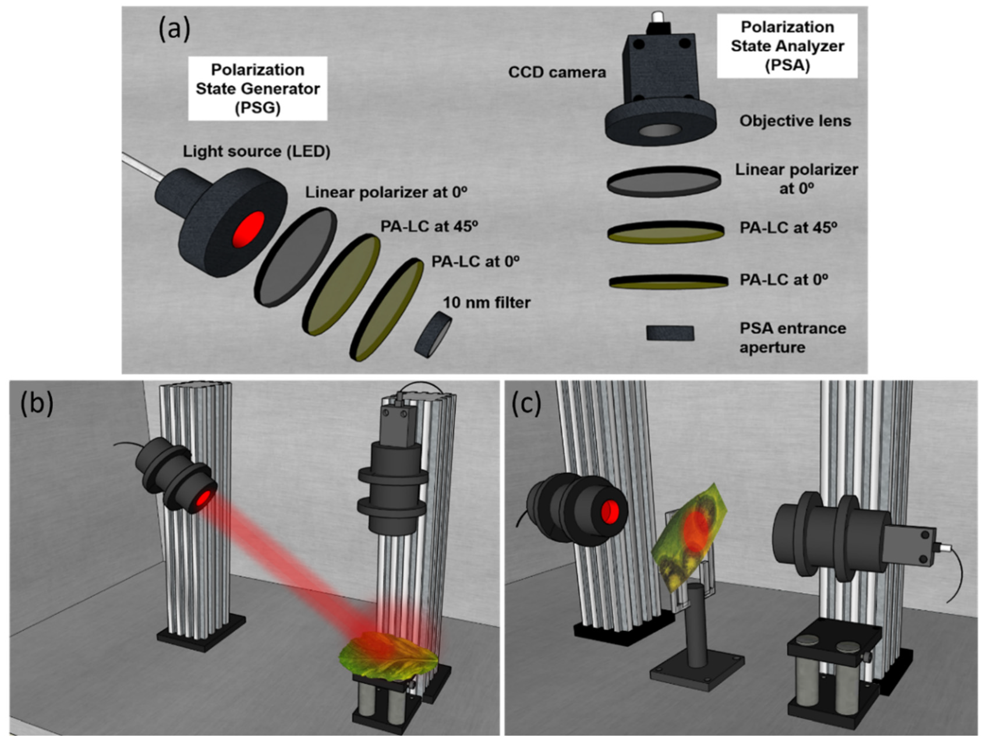
4.1. Experimental Setup Description: Complete Image Mueller Matrix Polarimeter

In this section, we describe the experimental setup used to obtain the experimental Mueller matrix images of the biological samples inspected in this work.

The polarimeter employed to obtain the experimental M of the analyzed samples is a complete imaging Mueller polarimeter. The polarimeter comprises two main parts: the Polarization State Generator (PSG) and the Polarization State Analyzer (PSA). The PSG and the PSA are composed of the respective series of optical elements (see Figure 2a) and devices, which allow to generate and analyze, respectively, any state of fully polarized light. In the case of the PSG, for being able to generate any state of polarization, it is comprised by a linear polarizer oriented at 0° with respect to the laboratory vertical and two Parallel Aligned Liquid Crystals (PA-LC) retarders oriented at 45° and 0° respectively. The PSA is comprised of the same optical elements as the PSG but located in inverse order (Figure 2a). To obtain the Mueller matrix images of the samples, a CCD camera is placed after the PSA to capture the intensity of the sample correspondent to each pixel. In addition, the PSG is illuminated with a light source which can work at different wavelengths in the visible spectrum (625 nm, 530 nm and 470 nm) allowing us to inspect different characteristics of samples. In particular, larger wavelengths polarimetrically interact with deeper tissues and shorter wavelengths mostly interacts with superficial tissues [66,67]. To reduce the spectrum of the different wavelengths of the LED source and to prevent artificial depolarization originated by the PA-LC’s performance dependence on said parameter, 10 nm filters for blue and green illumination are used. Note that, for an accurate experimental determination of the Mueller matrix of the samples, it is important to control external light sources, so that the only light source interacting with the sample is that present in the PSG. For this reason, experimental measurements of the Mueller matrix have been conducted in dark conditions in the laboratory.

The PSG and the PSA systems are set into two mobile arms, where their respective angles can be adjusted to achieve different measuring configurations, as defined by an angular-based variable Polarimeter. This capability allows us to measure samples at two measuring configurations: transmission and reflection.

To measure samples in the reflection configuration (see Figure 2b), the PSG is located at 34° with respect to the laboratory vertical and the PSA is at 0° with respect to the laboratory vertical, thus avoiding ballistic reflection (scattered light is measured). If the samples are thin enough, they are also measured in the transmission configuration (see Figure 2c), where the two arms (PSG and PSA) are located in the laboratory horizontal, one facing the other. This is the case for vegetal samples such as, for example, leaves. In turn, in the case of animal samples, due to the sample thickness and characteristics, we only use the above-mentioned reflection configuration. Last but not least, we want to note that we use the polarimeter in optimized conditions in order to minimize the noise amplification from intensity measures to the final experimental M. This has been done in terms of condition numbers and equally weighted variance metrics, by using the six based polarizing basis described in [68]. In this sense, the polarimeter provides an accuracy of 2% in the measurements [69].

In this section, we also provide the detailed characteristics of the employed setup. The illumination is provided by a Thorlabs LED source (LED4D211, operated by DC4104 drivers distributed by Thorlabs) complemented with 10 nm dielectric bandwidth filters FB530-10 and FB470-10 for green and blue wavelengths, respectively, from Thorlabs. The linear polarizers are a Glam-Thompson prism-based CASIX and a dichroic sheet polarizer from Meadowlark Optics in the case of the PSG and the PSA, respectively. The four PA-LC retarders are Variable Retarders with Temperature Control (LVR-200-400-700-1LTSC distributed by Meadowlark Optics). Finally, imaging is performed by means of a 35 mm focal length Edmund Optics TECHSPEC^® high resolution objective followed by an Allied Vision Manta G-504B CCD camera, with 5 Megapixel GigE Vision and Sony ICX655 CCD sensor, 2452(H) × 2056(V) resolution, and cell size of 3.45 µm × 3.45 µm, so that a spatial resolution of 22 µm is achieved.

4.2. Sample Description and Preparation

In this subsection, we provide the physiological description of the animal and vegetal samples inspected in this work as well as the preparation procedure for the measures. The different structural components of tissue are directly related to their polarimetric response. Therefore, different structures can generate different values in the polarimetric observables. For instance, birefringent properties leading to retardance in biological samples can be produced by the organization of some fibers such as collagen and elastin [24]. To allow us to interpret the results when inspecting the polarimetric observables of the different samples, here we provide a brief physiological analysis of the different animal and plant structures inspected.

The plant sample is a pathological grapevine (Vitis rupestris Scheele) leaf. It was obtained from a collaboration with the Botanical Institute of Barcelona and the Institute of Agrifood Research and Technology. The leaf sample showed symptoms of black rot disease. Black rot of grapes is caused by the Ascomycete Guignardia bidwellii (Ellis) Viala and Ravaz (Botryosphaeriales). Guignardia bidwellii is a hemibiotrophic endoparasite that affects all growing green vine parts [70]; i.e., mainly occurring on leaves and additionally including leaf petioles, flowers and bunch peduncles and pedicels, shoots and tendrils [71]. On shoots, petioles, and pedicels, spots appear as small, darkened depressions. Lesions appear one or two weeks after infection on the infected plant part. The spots are roughly round or slightly segmented, some millimeters in size, initially brown-reddish and darkening with age.

During the biotrophic stage of G. bidwellii, soon after infection, hyphae grow mainly between the leaf cuticle and the walls of the palisade parenchyma. They form a dense, two-dimensional mycelium with no visible disease symptoms occurring during this latent incubation period, which may extend to up to 12 days [72,73]. When a later transition to necrotrophic stage occurs, mycelium of G. bidwellii expands and colonizes all leaf tissues (including epidermis, mesophyll and vascular bundles), thus leading to an overall necrosis of the infected plant part. Leaf samples used in this study were all showing necrotic lesions corresponding to the necrotrophic stage, and latent lesions (i.e., the biotrophic stage) were neither observed nor analyzed.

Production of secondary metabolites including guignardic acid, phenguignardic acid, alaguignardic acid, (6S,9R)-vomifoliol, several guignardianones (A–F), and several guignarenones (A–D) have been reported to date to be produced by different Guignardia species, which have been potentially demonstrated to show phytotoxic effects on plant cells [71]. Specifically, only (6S,9R)-vomifoliol and guignarenones (A–D) are known to be produced by G. bidwellii [74]. However, their phytotoxic action is disputed and their role in the development of grapevine black rot has not yet been confirmed [71].

The animal samples correspond to an ex vivo chicken tendon and a biopsy from an ex vivo cow brain. They were obtained from a local slaughterhouse and no laboratory animals were used for the experiments; previous treatment and commercial use of the animal tissue were in accordance with Spanish legislation. The samples were stored at −16 °C after the acquisition and until the measurements.

Tendons are composed of parallel fascicles of collagen following the same directionality as the corresponding muscle. Both tendinous and its surrounding tissue (fascia and areolar fatty tissue corresponding to paratenon) are of mesodermal origin, while the tendon is composed of densely packed directional bundles of type I collagen. This organization creates a striated structure.

The brain sample corresponds to a coronal section taken in the crossroad between the posterior parietal lobe and the occipital lobe of a cow, approximately 2 cm from the rostral to the occipital pole. This section is composed of cortical grey matter (GM), which is a layered cell-rich structure, and subcortical white matter (WM), which is sparsely cellular and composed of bundles of nerve fibers that connect the cortex with other cortical areas or with subcortical structures (at this level, mainly thalamus).

As previously stated, the plant sample was measured in the transmission configuration whereas for the animal samples, the reflection configuration was employed. All the samples were measured at the three available wavelengths in the polarimeter. For simplicity, here we only present the results providing the best structure visualization of the polarimetric observables (corresponding to 470 nm).

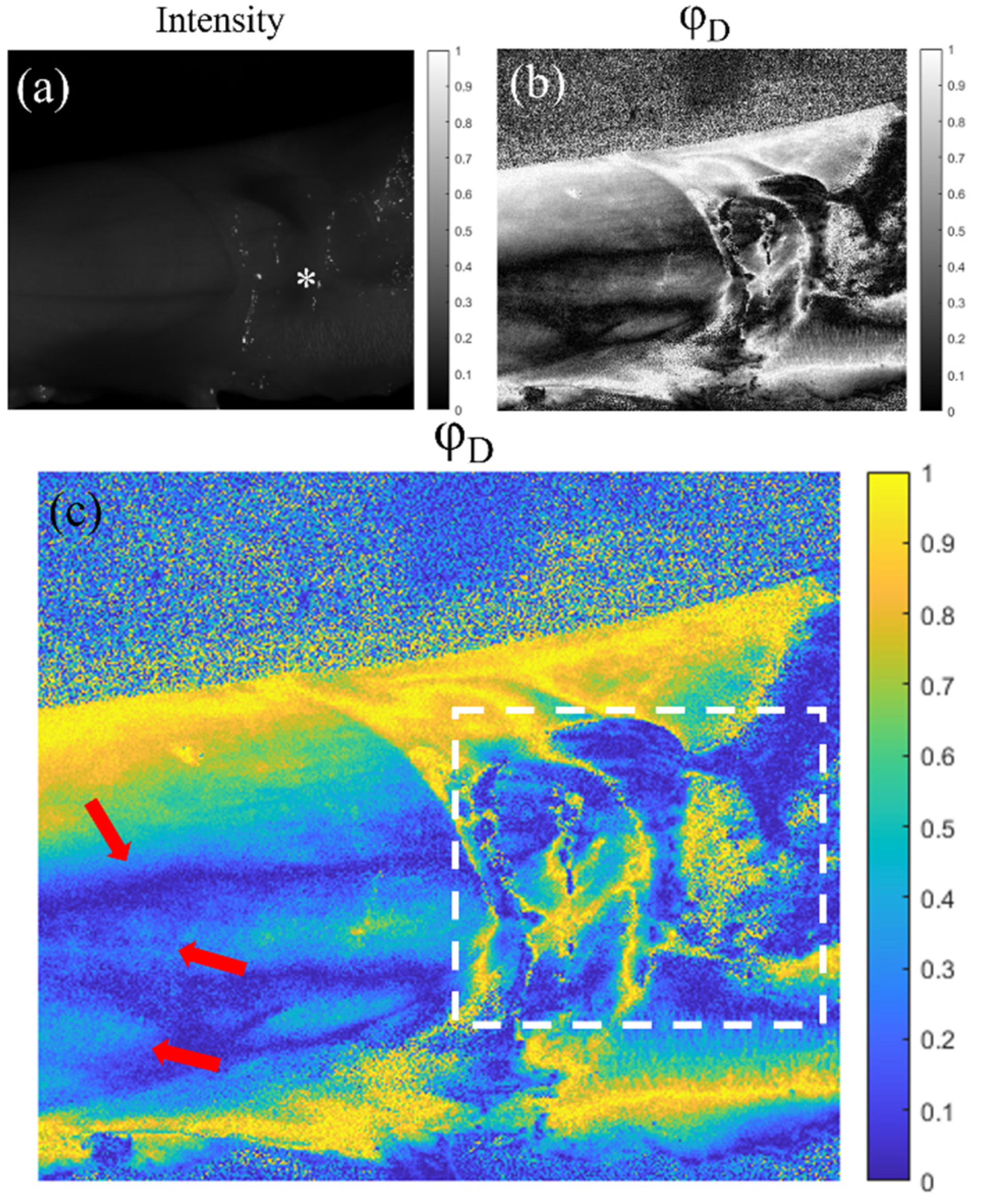
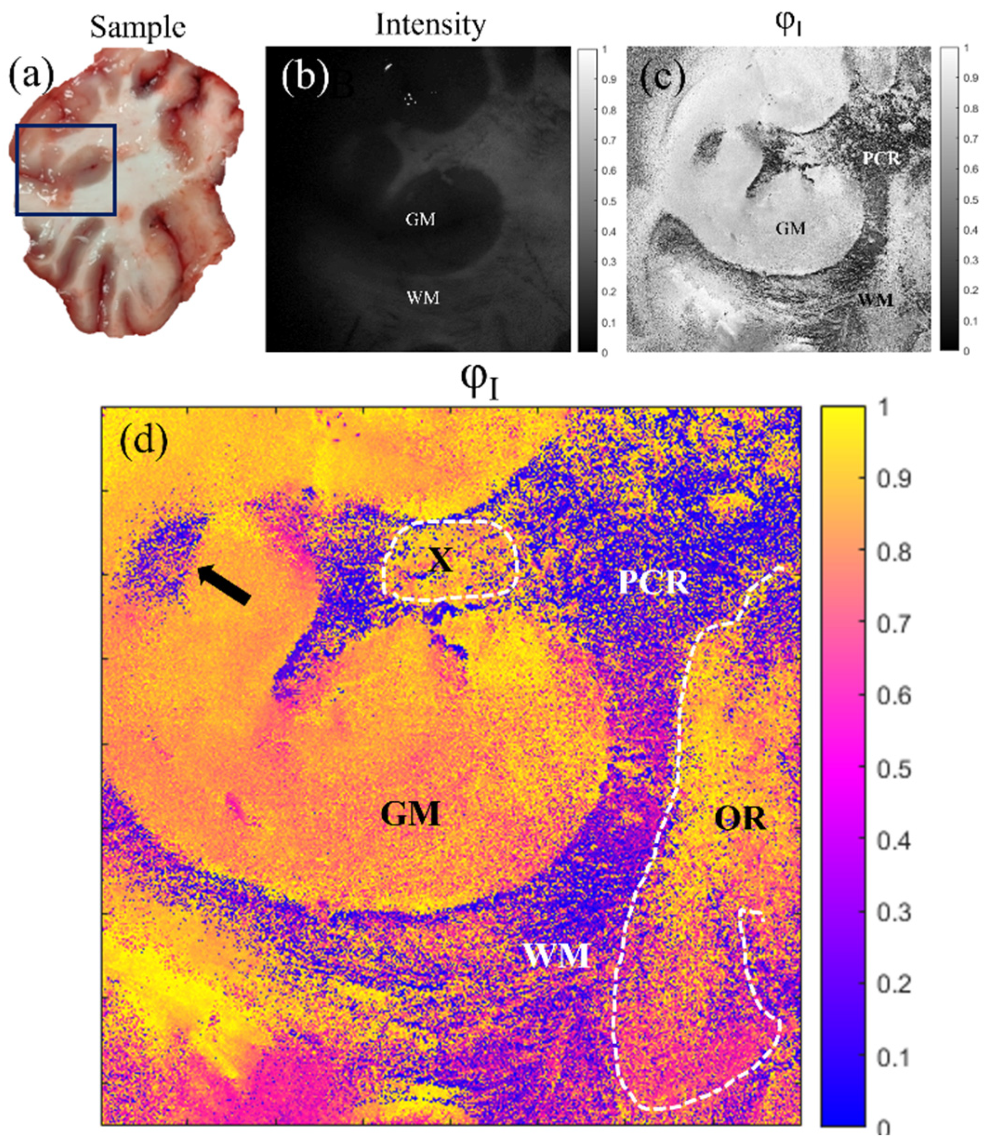
5. Application of the Mueller Matrix Parameterization to Polarimetric Imaging of Biological Tissues

In this section, we show the comparison between the standard intensity images of the studied samples (grapevine, tendon and brain; see Section 4) and some of the selected polarimetric observables’ images (R_I, ${\phi }_D$ and ${\phi }_I$; see Section 3). To highlight the potential of this set of observables calculated for each one of the studied samples, we provide the best observables-based images results in terms of tissue visualization in this section. Note that common biological samples present different polarimetric features and specific observables will focus on a particular characteristic inspecting such features. This limits the situation of retrieving all possible biological structures at the same time with a single polarimetric channel and, thus, multiple observables should be considered for a complete analysis of the sample under inspection. In turn, the sixteen arrow-decomposition-derived observables discussed in this work present a set of metrics studying the main polarimetric characteristics of samples (retardance, diattenuation and depolarization). In the following examples, from all calculated metrics (see Section 2), we choose to present the channels providing the best visualization of particular biological structures of interest.

On the one hand, in Figure 3, we show the results for the grapevine sample. In particular, we compare the intensity image (Figure 3a) of the plant sample and the polarimetric image correspondent to the entrance retardance parameter (R_I) (Figure 3b,c). We clearly observe the visualization enhancement between different structures of the plant associated with the polarimetric channel R_I when comparing Figure 3a,b. To benefit from the visual improvement related to colormaps, an image based on the entrance retardance parameter (R_I) is represented in Figure 3c in a different colormap than the grayscale in Figure 3b. For the following discussion, we will compare images (a) and (c).

In Figure 3c, we see how some structures almost invisible to the standard intensity image (Figure 3a) are clearly observable. For instance, in Figure 3c, we observe how different structures present in the leaf have different polarimetric responses—in this case in the entrance retardance value, which is translated in a different value of R_I. For instance, the pathological areas of the plant (see yellow arrows) present different retardance values than the rest of the healthy leaf lamina. That is, the structural changes produced in these necrotic areas of the leaf (see description in Section 4) produce a very different entrance retardance, R_I, behavior which allows us to have a great contrast between the not infected part of the plant and the necrotic stage of the pathology. Moreover, we also can differentiate the vascular structure of the plant, especially the highlighted primary veins (see yellow dashed rectangles). Note how the stated visualization improvement can be of interest for characterization as well as the pathological analysis of plants.

On the other hand, in Figure 4 and Figure 5, we show the results for the two studied animal samples. In the same way as with the plant sample, the polarimetric-observables-based images (both in grayscale and optimized colormap) are compared with the intensity image as a reference for each case.

In Figure 4, we see the images correspondent to the tendon sample. Figure 4a shows the standard intensity image of a tendon which is partially enveloped by fascia and areolar fatty tissue (indicated by the symbol * in the figure). In the polarimetric image (Figure 4c), which in these cases corresponds with the azimuth of the diattenuation (${\phi }_D$) observable, we are able to see structures almost not visible in the intensity channel (Figure 4a). In Figure 4b,c, we can appreciate a larger contrast between the fascia covering the right part of the tendon, where the different folds composing this structure have different azimuth values (see white rectangle in Figure 4). Moreover, the polarimetric channel ${\phi }_D$ also reveals a structure in the left part of the samples. These structures (see red arrows), hidden in the intensity image, are the boundaries between different fascicles inside the same tendon.

In this example, we show how the features of the directionality of fibers of a similar nature (collagen and elastic) may be useful to distinguish tissues with roughly similar compositions (tendon vs. peritenon; tendon strongly directional vs. peritenon looser and non-directional) but different organizations that are not readily identifiable at plain view. Although the direct application of that is not near in the future, it might be useful in the analysis of musculoskeletal diseases that imply long-term changes in motor strategies and, therefore, in the balance of mechanical forces that determine the organization of collagen-rich tissues [75,76].

Finally, in Figure 5, we provide the results for a coronal section of a cow brain (see a photograph of the sample in Figure 5a). Once again, the comparison is set between the standard intensity image (Figure 5b) and the best results for polarimetric images (azimuth of the entrance retarder, ${\phi }_I$; Figure 5c,d). In this vein, in Figure 5a,b, we can see two different structures in the brain: gray matter (GM) and white matter (WM); which present different compositions and functions in the brain. However, in the polarimetric images (Figure 5c,d), we are able to distinguish information about the sample structure which is not visible in the intensity channel. Firstly, the boundaries of the WM and the GM are better observed in the ${\phi }_I$ image, where we can see a region of WM (see black arrow in Figure 5d) clearly contrasted (note that this WM region is not distinguished in the intensity image and can be misclassified as GM). Importantly, other interesting structures are revealed in the ${\phi }_I$ image. In particular, in Figure 5d we can identify fiber tracts of the subcortical WM classified according to their directionality. This allows tracing the borders between the longitudinal (at this level) parietal radiations of the corona radiata (PCR in the figure), optical radiations (transversal, OR in the figure; framed with white dashed lines in the right of the figure) and specific fascicles probably corresponding to the dorsal visual processing pathway (for example, X in the figure; framed with white dashed lines).

Note that WM is composed of bundles of nerve fibers whose directionality is not identifiable macroscopically or with routine histochemistry, while specific techniques are time consuming or not easily reproducible. However, as we are sensible to different directionalities of the fibers composing the WM through the entrance retarder azimuth, ${\phi }_I$, this channel leads to the high contrast of these structures. Therefore, with this channel, we are capable of detecting information about the directionality of the fibers by means of macroscopic and nondestructive measures of the sample.

Brain connectivity and its functional expression is probably the present frontier of applied neuroscience, as there is no gold-standard technique for pathway mapping apart from peri-mortem tract-tracing injections that are not ethically suitable for the study of human connectivity [77]. Histology or ultrastructure-based methods can distinguish fiber orientation but are not useful for tracing long range tracts, which are only revealed by specific techniques of microdissection [78] where resolution in smaller areas is lost. In vivo diffusion magnetic resonance tractography is a widely used method that, however, lacks (by design) histological counterchecks and is unable to resolve crossing tracts, as well as providing amputated images in areas such as the corticospinal tract where terminations are unambiguous (see Ref. [77] for a review on the matter). There are two methodological studies that provide acceptable anatomical resolution after the ex vivo analysis of the directionality of white matter tracts in large specimens: optical coherence tomography [79] and Mueller matrix polarimetry [80]. Both studies demonstrate the ability to classify large tracts that are known to have different orientations (internal capsule, cerebral peduncles, fimbria, medial lemniscus, optic tract, see also Ref. [81]) and to resolve the limits between gray and white matter. Our approach is similar to that described by Felger et al. in Ref. [81] but shows a better resolution of tracts within the white matter.

6. Conclusions

In this work, we analyzed the suitability of a particular set of polarimetric observables in the framework of biological imaging, which are derived from the arrow decomposition of a Mueller matrix of a given sample: (1) the mean intensity coefficient ($m_{00}$) of $M_A$ of the measured Mueller matrix; (2) six angles (azimuth, ellipticity and retardance) determining the entrance and exit retarders $({\phi }_I,{\chi }_I,R_I,{\phi }_O,{\chi }_O,R_O)$, respectively; (3) three parameters (azimuth, ellipticity and diattenuation) determining the diattenuation vector $({\phi }_D,{\chi }_D,D)$; (4) three parameters (azimuth, ellipticity and polarizance) determining the polarizance vector $({\phi }_P,{\chi }_P,P)$; and (5) the three indices of polarimetric purity $(P_1,P_2,P_3)$. These conform to a polarimetric space of sixteen polarimetric properties which are reviewed in Section 2.

These sixteen metrics have been applied to test the suitability for the visualization enhancement of biological tissues. To experimentally determine such properties, we have measured the experimental Mueller matrix of the samples, thanks to a complete imaging polarimeter. In particular, the samples under study have been: (1) a vegetal sample, i.e., Vitis rupestris leaf; (2) an animal ex vivo sample, i.e., a chicken tendon; and (3) an animal ex vivo sample, i.e., a cow brain. The description of the samples as well as of the image polarimeter is provided in Section 3.

In Section 4, we have proved the potential of the methods by analyzing the experimental results for the above stated samples. In the case of the Vitis rupestris leaf, the entrance retardance parameter $(R_I)$ leads to the best visualization results, allowing for a clear visualization of the necrotic areas of the leaf. For the case of tendinous tissue, the best visualization is provided by the azimuth of the diattenuation $({\phi }_D)$, revealing the dichroic nature of the tissue and allowing for detecting the boundaries between different fascicles inside the same tendon. Finally, for the coronal section of the brain, the azimuth of the entrance retardance $({\phi }_I)$ was selected, with this channel revealing fiber tracts of the subcortical white matter classified according to their directionality.

The improved results in terms of structure visualization pave the way for new applications in the fields of biomedical and botanical areas. We think they offer new possibilities for the early detection of some pathologies or for fundamental physiological studies. Importantly, we want to highlight that with this technique we are able to clearly observe some structures, as is the case for different bundles within the subcortical white matter of the brain, which are difficult to describe both in vivo and postmortem and require time-consuming and not easily reproducible methods, such as microinjections or specific, highly destructive techniques for dissection. Importantly, the methods provided are non-invasive and could be applied in real time applications, being in numerous cases less expensive than other existing alternatives. Last but not least, these polarimetric methods can be combined with other well-known optical techniques [82,83,84] to help the early detection of pathologies. In this sense, structures showing retardance features seem to be ideal to be analyzed through the arrow metrics, as can be the case of tissues consisting of collagen (muscle, tendon, myotendinous junction, skin, brain and associated pathologies).

To summarize, we have demonstrated the excellent potential of these metrics to not only enhance the contrast between different relevant structures in biological samples (both of animal and vegetal origin) but also to show structures that are hidden by using basic imaging systems. These are very promising results in biological applications such as plant pathology detection or animal tissue recognition. Nevertheless, further research would be required to compare the utility of such metrics with other well-known polarimetric observables in order to find the best suited polarimetric observables in terms of sample visualization (including human studies), but further studies point out in the direction that suitability will strongly depend on specific samples.

References

1. Goldstein, D.H. Polarized Light, Revised and Expanded; CRC Press: Boca Raton, FL, USA, 2003; ISBN 9780203911587. [Google Scholar]
2. Gil, J.J.; Ossikovski, R. Polarized Light and the Mueller Matrix Approach; CRC Press: New York, NY, USA, 2022; ISBN 9780367815578. [Google Scholar]
3. Chipman, R.A. Polarimetry. In Handbook of Optics II; McGraw-Hill: New York, NY, USA, 1995; Chapter 22. [Google Scholar]
4. Sheppard, C.J.R.; Bendandi, A.; Le Gratiet, A.; Diaspro, A. Eigenvectors of Polarization Coherency Matrices. J. Opt. Soc. Am. A 2020, 37, 1143. [Google Scholar] [CrossRef] [PubMed]
5. Ignatenko, D.N.; Shkirin, A.V.; Lobachevsky, Y.P.; Gudkov, S.V. Applications of Mueller Matrix Polarimetry to Biological and Agricultural Diagnostics: A Review. Appl. Sci. 2022, 12, 5258. [Google Scholar] [CrossRef]
6. Li, J.; Liao, R.; Guan, C.; Wang, H.; Zhuo, Z.; Zeng, Y.; Ma, H. Particulate Mueller Matrix Polarimetry. Opt. Laser. Technol. 2023, 158, 108780. [Google Scholar] [CrossRef]
7. Gil, J.J.; Bernabeu, E. Depolarization and Polarization Indices of an Optical System. Opt. Acta Int. J. Opt. 1986, 33, 185–189. [Google Scholar] [CrossRef]
8. Lu, S.-Y.; Chipman, R.A. Interpretation of Mueller Matrices Based on Polar Decomposition. J. Opt. Soc. Am. A 1996, 13, 1106. [Google Scholar] [CrossRef]
9. Cloude, S. Group Theory and Polarisation Algebra. Optik 1986, 75, 26–36. [Google Scholar]
10. Ossikovski, R. Alternative Depolarization Criteria for Mueller Matrices. J. Opt. Soc. Am. A 2010, 27, 808. [Google Scholar] [CrossRef]
11. Tariq, A.; Li, P.; Chen, D.; Lv, D.; Ma, H. Physically Realizable Space for the Purity-Depolarization Plane for Polarized Light Scattering Media. Phys. Rev. Lett. 2017, 119, 033202. [Google Scholar] [CrossRef]
12. San José, I.; Gil, J.J. Invariant Indices of Polarimetric Purity: Generalized Indices of Purity for n × n Covariance Matrices. Opt. Commun. 2011, 284, 38–47. [Google Scholar] [CrossRef] [Green Version]
13. Ossikovski, R.; Vizet, J. Eigenvalue-Based Depolarization Metric Spaces for Mueller Matrices. J. Opt. Soc. Am. A 2019, 36, 1173. [Google Scholar] [CrossRef]
14. Van Eeckhout, A.; Lizana, A.; Garcia-Caurel, E.; Gil, J.J.; Sansa, A.; Rodríguez, C.; Estévez, I.; González, E.; Escalera, J.C.; Moreno, I.; et al. Polarimetric Imaging of Biological Tissues Based on the Indices of Polarimetric Purity. J. Biophotonics 2018, 11, e201700189. [Google Scholar] [CrossRef] [PubMed]
15. Rodríguez, C.; Garcia-Caurel, E.; Garnatje, T.; Serra i Ribas, M.; Luque, J.; Campos, J.; Lizana, A. Polarimetric Observables for the Enhanced Visualization of Plant Diseases. Sci. Rep. 2022, 12, 14743. [Google Scholar] [CrossRef] [PubMed]
16. Khan, S.; Qadir, M.; Khalid, A.; Ashraf, S.; Ahmad, I. Characterization of Cervical Tissue Using Mueller Matrix Polarimetry. Lasers Med. Sci. 2023, 38, 46. [Google Scholar] [CrossRef] [PubMed]
17. Ahmad, I.; Gribble, A.; Ikram, M.; Pop, M.; Vitkin, A. Polarimetric Assessment of Healthy and Radiofrequency Ablated Porcine Myocardial Tissue. J. Biophotonics 2016, 9, 750–759. [Google Scholar] [CrossRef]
18. Canabal-Carbia, M.; Rodriguez, C.; Estévez, I.; Van Eeckout, A.; González-Arnay, E.; García-Caurel, E.; Garnatje, T.; Lizana, A.; Campos, J. Enhancing Biological Tissue Structures Visualization through Polarimetric Parameters. In Proceedings of the SPIE 1238205, San Francisco, CA, USA, 28 January–2 February 2023; p. 16. [Google Scholar] [CrossRef]
19. Borovkova, M.; Trifonyuk, L.; Ushenko, V.; Dubolazov, O.; Vanchulyak, O.; Bodnar, G.; Ushenko, Y.; Olar, O.; Ushenko, O.; Sakhnovskiy, M.; et al. Mueller-Matrix-Based Polarization Imaging and Quantitative Assessment of Optically Anisotropic Polycrystalline Networks. PLoS ONE 2019, 14, e0214494. [Google Scholar] [CrossRef] [Green Version]
20. Clark, A.G.; Vignjevic, D.M. Modes of Cancer Cell Invasion and the Role of the Microenvironment. Curr. Opin. Cell Biol. 2015, 36, 13–22. [Google Scholar] [CrossRef] [Green Version]
21. Wood, M.F.G.; Ghosh, N.; Wallenburg, M.A.; Li, S.-H.; Weisel, R.D.; Wilson, B.C.; Li, R.-K.; Vitkin, I.A. Polarization Birefringence Measurements for Characterizing the Myocardium, Including Healthy, Infarcted, and Stem-Cell-Regenerated Tissues. J. Biomed. Opt. 2010, 15, 047009. [Google Scholar] [CrossRef] [Green Version]
22. Hogan, B.T.; Ushenko, V.A.; Syvokorovskaya, A.-V.; Dubolazov, A.V.; Vanchulyak, O.Y.; Ushenko, A.G.; Ushenko, Y.A.; Gorsky, M.P.; Tomka, Y.; Kuznetsov, S.L.; et al. 3D Mueller Matrix Reconstruction of the Optical Anisotropy Parameters of Myocardial Histopathology Tissue Samples. Front. Phys. 2021, 9, 737866. [Google Scholar] [CrossRef]
23. Palevitz, B.A.; Hepler, P.K. Cellulose Microfibril Orientation and Cell Shaping in Developing Guard Cells of Allium: The Role of Microtubules and Ion Accumulation. Planta 1976, 132, 71–93. [Google Scholar] [CrossRef]
24. Wang, L.V.; Coté, G.L.; Jacques, S.L. Special Section Guest Editorial. J. Biomed. Opt. 2002, 7, 278. [Google Scholar] [CrossRef] [Green Version]
25. Peyvasteh, M.; Dubolazov, A.; Popowv, A.; Ushenko, A.; Ushenko, Y.; Meglinski, I. Two-point Stokes vector diagnostic approach for characterization of optically anisotropic biological tissues. J. Phys. D Appl. Phys. 2020, 53, 395401. [Google Scholar] [CrossRef]
26. Ghosh, N.; Vitkin, I.A. Tissue Polarimetry: Concepts, Challenges, Applications, and Outlook. J. Biomed. Opt. 2011, 16, 110801. [Google Scholar] [CrossRef] [PubMed] [Green Version]
27. Borovkova, M.; Peyvasteh, M.; Dubolazov, O.; Ushenko, Y.; Ushenko, V.; Bykov, A.; Deby, S.; Rehbinder, J.; Novikova, T.; Meglinski, I. Complementary Analysis of Mueller-Matrix Images of Optically Anisotropic Highly Scattering Biological Tissues. J. Eur. Opt. Soc.-Rapid Publ. 2018, 14, 20. [Google Scholar] [CrossRef]
28. Shtein, I.; Shelef, Y.; Marom, Z.; Zelinger, E.; Schwartz, A.; Popper, Z.A.; Bar-On, B.; Harpaz-Saad, S. Stomatal Cell Wall Composition: Distinctive Structural Patterns Associated with Different Phylogenetic Groups. Ann. Bot. 2017, 119, 1021–1033. [Google Scholar] [CrossRef] [PubMed] [Green Version]
29. Ali, Z.; Mahmood, T.; Shahzad, A.; Iqbal, M.; Ahmad, I. Assessment of Tissue Pathology Using Optical Polarimetry. Lasers Med. Sci. 2022, 37, 1907–1919. [Google Scholar] [CrossRef] [PubMed]
30. Badieyan, S.; Ameri, A.; Razzaghi, M.R.; Rafii-Tabar, H.; Sasanpour, P. Mueller Matrix Imaging of Prostate Bulk Tissues; Polarization Parameters as a Discriminating Benchmark. Photodiagnosis Photodyn. Ther. 2019, 26, 90–96. [Google Scholar] [CrossRef] [PubMed]
31. Van Eeckhout, A.; Garcia-Caurel, E.; Ossikovski, R.; Lizana, A.; Rodríguez, C.; González-Arnay, E.; Campos, J. Depolarization Metric Spaces for Biological Tissues Classification. J. Biophotonics 2020, 13, e202000083. [Google Scholar] [CrossRef]
32. Ivanov, D.; Dremin, V.; Borisova, E.; Bykov, A.; Novikova, T.; Meglinski, I.; Ossikovski, R. Polarization and Depolarization Metrics as Optical Markers in Support to Histopathology of Ex Vivo Colon Tissue. Biomed. Opt. Express 2021, 12, 4560. [Google Scholar] [CrossRef]
33. Pierangelo, A.; Benali, A.; Antonelli, M.-R.; Novikova, T.; Validire, P.; Gayet, B.; De Martino, A. Ex-Vivo Characterization of Human Colon Cancer by Mueller Polarimetric Imaging. Opt. Express 2011, 19, 1582. [Google Scholar] [CrossRef]
34. Rodríguez, C.; Van Eeckhout, A.; Ferrer, L.; Garcia-Caurel, E.; González-Arnay, E.; Campos, J.; Lizana, A. Polarimetric Data-Based Model for Tissue Recognition. Biomed. Opt. Express 2021, 12, 4852. [Google Scholar] [CrossRef]
35. Wan, J.; Dong, Y.; Xue, J.-H.; Lin, L.; Du, S.; Dong, J.; Yao, Y.; Li, C.; Ma, H. Polarization-Based Probabilistic Discriminative Model for Quantitative Characterization of Cancer Cells. Biomed. Opt. Express 2022, 13, 3339. [Google Scholar] [CrossRef] [PubMed]
36. Canabal-Carbia, M.; Van Eeckhout, A.; Rodríguez, C.; González-Arnay, E.; Estévez, I.; Gil, J.J.; García-Caurel, E.; Ossikovski, R.; Campos, J.; Lizana, A. Depolarizing Metrics in the Biomedical Field: Vision Enhancement and Classification of Biological Tissues. J. Innov. Opt. Health Sci. 2023, 2330004, 1–17. [Google Scholar] [CrossRef]
37. Chue-Sang, J.; Holness, N. Use of Mueller Matrix Colposcopy in the Characterization of Cervical Collagen Anisotropy. J. Biomed. Opt. 2018, 23, 1. [Google Scholar] [CrossRef] [PubMed] [Green Version]
38. Sprenger, J.; Murray, C.; Lad, J.; Jones, B.; Thomas, G.; Nofech-Mozes, S.; Khorasani, M.; Vitkin, A. Toward a Quantitative Method for Estimating Tumour-Stroma Ratio in Breast Cancer Using Polarized Light Microscopy. Biomed. Opt. Express 2021, 12, 3241. [Google Scholar] [CrossRef]
39. Ramella-Roman, J.C.; Saytashev, I.; Piccini, M. A Review of Polarization-Based Imaging Technologies for Clinical and Preclinical Applications. J. Opt. 2020, 22, 123001. [Google Scholar] [CrossRef]
40. Trifonyuk, L.; Sdobnov, A.; Baranowski, W.; Ushenko, V.; Olar, O.; Dubolazov, A.; Pidkamin, L.; Sidor, M.; Vanchuliak, O.; Motrich, A.; et al. Differential Mueller Matrix Imaging of Partially Depolarizing Optically Anisotropic Biological Tissues. Lasers Med. Sci. 2020, 35, 877–891. [Google Scholar] [CrossRef] [Green Version]
41. Van Eeckhout, A.; Garcia-Caurel, E.; Garnatje, T.; Escalera, J.C.; Durfort, M.; Vidal, J.; Gil, J.J.; Campos, J.; Lizana, A. Polarimetric Imaging Microscopy for Advanced Inspection of Vegetal Tissues. Sci. Rep. 2021, 11, 3913. [Google Scholar] [CrossRef]
42. Van Eeckhout, A.; Garcia-Caurel, E.; Garnatje, T.; Durfort, M.; Escalera, J.C.; Vidal, J.; Gil, J.J.; Campos, J.; Lizana, A. Depolarizing Metrics for Plant Samples Imaging. PLoS ONE 2019, 14, e0213909. [Google Scholar] [CrossRef] [Green Version]
43. Savenkov, S.N.; Muttiah, R.S.; Oberemok, E.A.; Priezzhev, A.V.; Kolomiets, I.S.; Klimov, A.S. Measurement and Interpretation of Mueller Matrices of Barley Leaves. Quantum Elec. 2020, 50, 55–60. [Google Scholar] [CrossRef]
44. Al Bugami, B.; Su, Y.; Rodríguez, C.; Lizana, A.; Campos, J.; Durfort, M.; Ossikovski, R.; Garcia-Caurel, E. Characterization of Vine, Vitis Vinifera, Leaves by Mueller Polarimetric Microscopy. Thin Solid Films 2023, 764, 139594. [Google Scholar] [CrossRef]
45. Rodríguez, C.; Van Eeckhout, A.; Garcia-Caurel, E.; Lizana, A.; Campos, J. Automatic Pseudo-Coloring Approaches to Improve Visual Perception and Contrast in Polarimetric Images of Biological Tissues. Sci. Rep. 2022, 12, 18479. [Google Scholar] [CrossRef] [PubMed]
46. Patty, C.H.L.; Luo, D.A.; Snik, F.; Ariese, F.; Buma, W.J.; ten Kate, I.L.; van Spanning, R.J.M.; Sparks, W.B.; Germer, T.A.; Garab, G.; et al. Imaging Linear and Circular Polarization Features in Leaves with Complete Mueller Matrix Polarimetry. Biochim. Biophys. Acta (BBA) Gen. Subj. 2018, 1862, 1350–1363. [Google Scholar] [CrossRef] [PubMed]
47. Rodríguez-Núñez, O.; Schucht, P.; Hewer, E.; Novikova, T.; Pierangelo, A. Polarimetric Visualization of Healthy Brain Fiber Tracts under Adverse Conditions: Ex Vivo Studies. Biomed. Opt. Express 2021, 12, 6674. [Google Scholar] [CrossRef] [PubMed]
48. Schucht, P.; Lee, H.R.; Mezouar, H.M.; Hewer, E.; Raabe, A.; Murek, M.; Zubak, I.; Goldberg, J.; Kovari, E.; Pierangelo, A.; et al. Visualization of White Matter Fiber Tracts of Brain Tissue Sections With Wide-Field Imaging Mueller Polarimetry. IEEE Trans. Med. Imaging 2020, 39, 4376–4382. [Google Scholar] [CrossRef]
49. Ushenko, V.A.; Hogan, B.T.; Dubolazov, A.; Piavchenko, G.; Kuznetsov, S.L.; Ushenko, A.G.; Ushenko, Y.O.; Gorsky, M.; Bykov, A.; Meglinski, I. 3D Mueller Matrix Mapping of Layered Distributions of Depolarisation Degree for Analysis of Prostate Adenoma and Carcinoma Diffuse Tissues. Sci. Rep. 2021, 11, 5162. [Google Scholar] [CrossRef]
50. Ahmad, I.; Khaliq, A.; Iqbal, M.; Khan, S. Mueller Matrix Polarimetry for Characterization of Skin Tissue Samples: A Review. Photodiagnosis Photodyn. Ther. 2020, 30, 101708. [Google Scholar] [CrossRef]
51. Du, E.; He, H.; Zeng, N.; Sun, M.; Guo, Y.; Wu, J.; Liu, S.; Ma, H. Mueller Matrix Polarimetry for Differentiating Characteristic Features of Cancerous Tissues. J. Biomed. Opt. 2014, 19, 076013. [Google Scholar] [CrossRef]
52. Kupinski, M.; Boffety, M.; Goudail, F.; Ossikovski, R.; Pierangelo, A.; Rehbinder, J.; Vizet, J.; Novikova, T. Polarimetric Measurement Utility for Pre-Cancer Detection from Uterine Cervix Specimens. Biomed. Opt. Express 2018, 9, 5691. [Google Scholar] [CrossRef]
53. Van Eeckhout, A.; González, E.; Escalera, J.C.; Moreno, I.; Campos, J.; Zhang, H.; Ossikovski, R.; Lizana, A.; Garcia-Caurel, E.; Gil, J.J.; et al. Indices of Polarimetric Purity to Enhance the Image Quality in Biophotonics Applications. In Proceedings of the SPIE 10685, Strasbourg, France, 22–26 April 2018; p. 9. [Google Scholar] [CrossRef]
54. Ushenko, V.; Sdobnov, A.; Syvokorovskaya, A.; Dubolazov, A.; Vanchulyak, O.; Ushenko, A.; Ushenko, Y.; Gorsky, M.; Sidor, M.; Bykov, A.; et al. 3D Mueller-Matrix Diffusive Tomography of Polycrystalline Blood Films for Cancer Diagnosis. Photonics 2018, 5, 54. [Google Scholar] [CrossRef] [Green Version]
55. Ushenko, V.A.; Hogan, B.T.; Dubolazov, A.; Grechina, A.V.; Boronikhina, T.V.; Gorsky, M.; Ushenko, A.G.; Ushenko, Y.O.; Bykov, A.; Meglinski, I. Embossed Topographic Depolarisation Maps of Biological Tissues with Different Morphological Structures. Sci. Rep. 2021, 11, 3871. [Google Scholar] [CrossRef]
56. Gil, J.J. Transmittance Constraints in Serial Decompositions of Depolarizing Mueller Matrices: The Arrow Form of a Mueller Matrix. J. Opt. Soc. Am. A 2013, 30, 701–707. [Google Scholar] [CrossRef]
57. Gil, J.J.; San José, I. Reduced Form of a Mueller Matrix. J. Mod. Opt. 2016, 63, 1579–1583. [Google Scholar] [CrossRef] [Green Version]
58. Ossikovski, R. Analysis of Depolarizing Mueller Matrices through a Symmetric Decomposition. J. Opt. Soc. Am. A 2009, 26, 1109. [Google Scholar] [CrossRef] [PubMed]
59. Xing, Z.-F. On the Deterministic and Non-Deterministic Mueller Matrix. J. Mod. Opt. 1992, 39, 461–484. [Google Scholar] [CrossRef]
60. Robson, B.A. The Theory of Polarization Phenomena; Clarendon Press: Oxford, UK, 1975. [Google Scholar]
61. Sekera, Z. Scattering Matrices and Reciprocity Relationships for Various Representations of the State of Polarization. J. Opt. Soc. Am. 1966, 56, 1732. [Google Scholar] [CrossRef]
62. Schönhofer, A.; Kuball, H.-G. Symmetry Properties of the Mueller Matrix. Chem. Phys. 1987, 115, 159–167. [Google Scholar] [CrossRef]
63. Gil, J.J. Components of Purity of a Mueller Matrix. J. Opt. Soc. Am. A 2011, 28, 1578. [Google Scholar] [CrossRef]
64. Gil, J.J. Invariant Quantities of a Mueller Matrix under Rotation and Retarder Transformations. J. Opt. Soc. Am. A 2016, 33, 52–58. [Google Scholar] [CrossRef] [Green Version]
65. Gil, J.J. Physical Quantities Involved in a Mueller Matrix. In Proceedings of the SPIE 9853, Baltimore Chenault, MD, USA, 17–21 April 2016; p. 985302. [Google Scholar] [CrossRef]
66. Jacquemoud, S.; Ustin, S. Leaf Optical Properties; Cambridge University Press: Cambridge, UK, 2019; ISBN 9781108686457. [Google Scholar]
67. Mustafa, F.H.; Jaafar, M.S. Comparison of Wavelength-Dependent Penetration Depths of Lasers in Different Types of Skin in Photodynamic Therapy. Indian J. Phys. 2013, 87, 203–209. [Google Scholar] [CrossRef]
68. Peinado, A.; Lizana, A.; Vidal, J.; Iemmi, C.; Campos, J. Optimization and Performance Criteria of a Stokes Polarimeter Based on Two Variable Retarders. Opt. Express 2010, 18, 9815. [Google Scholar] [CrossRef]
69. Peinado, A. Analysis, Optimization and Implementation of a Variable Retardance Based Polarimeter; Universitat Autònoma de Barcelona: Barcelona, Spain, 2014. [Google Scholar]
70. De Silva, N.; Lumyong, S.; Hyde, K.D.; Bulgakov, T.; Philips, A.J.L.; Yan, J. Mycosphere Essays 9: Defining Biotrophs and Hemibiotrophs. Mycosphere 2016, 7, 545–559. [Google Scholar] [CrossRef]
71. Szabó, M.; Csikász-Krizsics, A.; Dula, T.; Farkas, E.; Roznik, D.; Kozma, P.; Deák, T. Black Rot of Grapes (Guignardia bidwellii)—A Comprehensive Overview. Horticulturae 2023, 9, 130. [Google Scholar] [CrossRef]
72. Ullrich, C.I.; Kleespies, R.G.; Enders, M.; Koch, E. Biology of the Black Rot Pathogen, Guignardia bidwellii, Its Development in Susceptible Leaves of Grapevine Vitis Vinifera. J. Kulturflanzen 2009, 61, 82–90. [Google Scholar]
73. Kuo, K.; Hoch, H.C. The Parasitic Relationship between Phyllosticta Ampelicidaand Vitis Vinifera. Mycologia 1996, 88, 626–634. [Google Scholar] [CrossRef]
74. Sommart, U.; Rukachaisirikul, V.; Trisuwan, K.; Tadpetch, K.; Phongpaichit, S.; Preedanon, S.; Sakayaroj, J. Tricycloalternarene Derivatives from the Endophytic Fungus Guignardia Bidwellii PSU-G11. Phytochem. Lett. 2012, 5, 139–143. [Google Scholar] [CrossRef]
75. Rosin, N.L.; Agabalyan, N.; Olsen, K.; Martufi, G.; Gabriel, V.; Biernaskie, J.; Di Martino, E.S. Collagen Structural Alterations Contribute to Stiffening of Tissue after Split-Thickness Skin Grafting. Wound Repair Regen. 2016, 24, 263–274. [Google Scholar] [CrossRef]
76. Chen, P.; Wang, A.; Haynes, W.; Landao-Bassonga, E.; Lee, C.; Ruan, R.; Breidahl, W.; Shiroud Heidari, B.; Mitchell, C.A.; Zheng, M. A Bio-Inductive Collagen Scaffold That Supports Human Primary Tendon-Derived Cell Growth for Rotator Cuff Repair. J. Orthop. Transl. 2021, 31, 91–101. [Google Scholar] [CrossRef]
77. Charvet, C.J. Mapping Human Brain Pathways: Challenges and Opportunities in the Integration of Scales. Brain Behav. Evol. [CrossRef]
78. Agrawal, A.; Kapfhammer, J.P.; Kress, A.; Wichers, H.; Deep, A.; Feindel, W.; Sonntag, V.K.H.; Spetzler, R.F.; Preul, M.C. Josef Klingler’s Models of White Matter Tracts: Influences on Neuroanatomy, Neurosurgery, and Neuroimaging. Neurosurgery 2011, 69, 238–254. [Google Scholar] [CrossRef]
79. Wang, H.; Black, A.J.; Zhu, J.; Stigen, T.W.; Al-Qaisi, M.K.; Netoff, T.I.; Abosch, A.; Akkin, T. Reconstructing Micrometer-Scale Fiber Pathways in the Brain: Multi-Contrast Optical Coherence Tomography Based Tractography. Neuroimage 2011, 58, 984–992. [Google Scholar] [CrossRef] [Green Version]
80. Felger, L.; Rodríguez-Núñez, O.; Gros, R.; Maragkou, T.; McKinley, R.; Moriconi, S.; Murek, M.; Zubak, I.; Novikova, T.; Pierangelo, A.; et al. Robustness of the Wide-Field Imaging Mueller Polarimetry for Brain Tissue Differentiation and White Matter Fiber Tract Identification in a Surgery-like Environment: An Ex Vivo Study. Biomed. Opt. Express 2023, 14, 2400. [Google Scholar] [CrossRef]
81. Mandonnet, E.; Sarubbo, S.; Petit, L. The Nomenclature of Human White Matter Association Pathways: Proposal for a Systematic Taxonomic Anatomical Classification. Front. Neuroanat. 2018, 12, 94. [Google Scholar] [CrossRef] [PubMed] [Green Version]
82. Helmchen, F.; Denk, W. Deep Tissue Two-Photon Microscopy. Nat. Methods 2005, 2, 932–940. [Google Scholar] [CrossRef] [PubMed]
83. Arano-Martinez, J.A.; Martínez-González, C.L.; Salazar, M.I.; Torres-Torres, C. A Framework for Biosensors Assisted by Multiphoton Effects and Machine Learning. Biosensors 2022, 12, 710. [Google Scholar] [CrossRef] [PubMed]
84. Raja, H.; Akram, M.U.; Hassan, T.; Ramzan, A.; Aziz, A.; Raja, H. Glaucoma Detection Using Optical Coherence Tomography Images: A Systematic Review of Clinical and Automated Studies. IETE J. Res. 2022, 1–21. [Google Scholar] [CrossRef]
Figure 1. Arrow decomposition of a Mueller matrix. For any incident polarization state, with Stokes vector S, the effect of any given Mueller matrix M is equivalent to that of a serial combination of an entrance retarder  M R I , the arrow form  M A  associated with M and an exit retarder  M R O .
Photonics 10 00669 g001
Figure 2. Three-dimensional representation of (a) the PSG and PSA optical components; the complete image Mueller polarimeter configurations used in this work; (b) reflection configuration; and (c) transmission configuration. Image reproduced from Ref. [15].
Photonics 10 00669 g002
Figure 3. Images of the pathological grapevine sample for the 470 nm illumination wavelength. (a) Intensity image; (b,c) images of the RI polarimetric channel with different colormaps (indicated on the right of the image). The yellow arrows indicate the necrotic lesions of the leaf and, the yellow dashed rectangles indicate some of the primary veins in the leaf.
Photonics 10 00669 g003
Figure 4. Images of the tendon sample for the 470 nm illumination wavelength. (a) Intensity image, (b,c) azimuth of the diattenuation,  φ D , images with different colormaps (indicated on the right of each image). The tendon is partially (*) enveloped by fascia and areolar fatty tissue corresponding to paratenon. Red arrows in (c) indicate boundaries between different fascicles inside the same tendon.
Photonics 10 00669 g004
Figure 5. Images of a coronal section of a cow brain sample for the 470 nm illumination wavelength. The sample corresponds to a section taken in the crossroad between the posterior parietal and occipital lobes with cortical grey matter (GM) and subcortical white matter (WM) fibers correspondent to different types of radiation; parietal radiations of the corona radiata (PCR) and optical radiations (OR). (a) Macroscopic plain view of the full cut of the sample, (b) intensity image, (c,d) entrance retarder azimuth images,  φ I , with different colormaps (indicated on the right of each image).
Photonics 10 00669 g005
Disclaimer/Publisher’s Note: The statements, opinions and data contained in all publications are solely those of the individual author(s) and contributor(s) and not of MDPI and/or the editor(s). MDPI and/or the editor(s) disclaim responsibility for any injury to people or property resulting from any ideas, methods, instructions or products referred to in the content.