Abstract
This work presents a methodology that relies on the application of the radial basis functions network (RBF)-based feedback control algorithms to a pharmaceutical crystallization process. Within the scope of the model-based evaluation of the proposed strategy, firstly strategies for the data treatment, data structure and the training methods reflecting the possible scenarios in the industry (Moving Window, Growing Window and Golden Batch strategies) were introduced. This was followed by the incorporation of such RBF strategies within a soft sensor application and a nonlinear predictive data-driven control application. The performance of the RBF control strategies was tested for the undisturbed cases as well as in the presence of disturbances in the process. The promising results from both RBF soft sensor control and the RBF predictive control demonstrated great potential of these techniques for the control of the crystallization process. In particular, both Moving Window and Golden Batch strategies performed the best results for an RBF soft sensor, and the Growing Window outperformed the remaining methodologies for predictive control.
1. Introduction
The introduction of more advanced control methodologies within the pharmaceutical industry was caused by two reasons, which in turn were mostly consequences of the U.S. Food and Drug Administration (FDA) guidelines [1,2]. Firstly, the demand for enhanced sustainable and more reliable processes created the opportunity to implement more advanced control techniques that could deal with the newly accepted process constraints and multi-objective criteria. Secondly, the implementation of process analytical tools (PAT) allowed for pharmaceutical processes to acquire online data that could provide a real-time understanding of the process operations [3,4]. In addition, control has become a central part of every crystallization process that has two or more polymorphs involved, due to incidents caused by the lack of design knowledge or control expertise within said polymorphic metastable zone (namely the cases of the active pharmaceutical ingredients (APIs): Thalidomide [5,6] and Ritonavir [7]).
Regarding crystallization processes, there are two main approaches to control implementation: model-free control and model-based control. The model-free control can be defined as the traditional proportional-integral (PI) controller that operates through a feedback loop, following a predefined profile of setpoints for batch crystallization processes. An example is the implementation of the direct nucleation control (DNC) [8] strategy, where real-time measurements, for example using a focused beam reflectance measurement (FBRM) sensor, are being collected and the total number of particles (in terms of total chord counts) is controlled (through solvent addition or manipulation of the cooling rate). Yang et al. [9] recently applied the same DNC methodology to a one-stage and a two-stage mixed-suspension, mixed-product-removal (MSMPR) crystallizer, with measurement data being provided through the implementation of the FBRM technique. In addition to achieving the desired chord length distribution (CLD), it was showed that the combination of the DNC methodology with an MSMPR crystallizer could reduce the start-up time operation, while effectively being able to suppress any given disturbance.
The model-based approach involves the application of crystallization process models and optimization algorithms to achieve tight quality control. Mesbah et al. [10] developed a model-based methodology to control the growth rate below a specified constrained value. The controlled variable was then correlated with measured crystal size distribution (CSD) using an extended Luenberger-type observer. With the designed control system, the yield and product quality were improved. Using a phase diagram, solute concentration can also be calculated, assisted by an analytical CSD estimator [11], or by using the concentration control strategy in a hierarchical structure [12]. Trifkovic et al. [13] proposed a new way to directly calculate the nucleation and growth rates from the moments of the particle population density obtained by FBRM. Assembling the mass and energy balances, and the population balance equation (PBE), the optimal anti-solvent flow rate was achieved using both a single and a multi-objective optimization algorithm.
Due to the fact that crystallization processes are difficult to model, hybrid approaches have been also used by some authors. Suárez et al. [14] applied a data-driven predictive control model methodology for the fed-batch control of sugar crystallization. A neural network (NN) hidden layer was used as the input-output model approach, with the inputs being the current supersaturation, pressure, temperature, flow rate and the stirrer power. A model predictive control (MPC) was applied to the optimization of the online model generation, with the target of optimizing the final CSD. Suárez et al. [14] showed that by dividing the process into 4 checkpoints where the target CSD has to satisfy the desired CSD, the final target CSD could be achieved with process uncertainty and disturbances. Moreover, an a priori model was required, and no initial data were demanded for the case scenario. More recently, Daosud et al. [15] applied an inverse NN with the Levenberg–Marquardt training data approach and tan-sigmoidal hidden layers to the crystallization of citric acid. Two hidden layers were used, performing a total of 4 layers of NN. The final results show an improved performance of the inverse NN against a traditional feedback PI controller.
In the early stages of a new API process design, often historic data and process understanding can be not sufficiently advanced, leading to trial and error experiments in order to scope quickly solutions/procedures for API isolation (crystallization and chromatography) under a strict time window (due to market pressure). However, due to the early stages of the new process, uncertainty within the product attributes prior to the current process point is to be expected, and disturbances cannot be disregarded. Data-driven approaches have shown to provide effective results for cases in which process data can be provided (online or offline), and the system is recognized to be too difficult to model/understand or/and the data sets for inputs and outputs are too large to handle, from a modeling perspective [16,17].
Radial basis functions (RBF) neural networks were firstly introduced in 1988 by Broomhead et al. [18], and have been adopted in different scenarios for simplifying complex models [19], soft sensor modeling [20] and nonlinear control strategies [21,22]. The embodiment of this multilayer network that correlates input and output data (measurements and/or historic data) through a set of hidden nodes (containing different possible sets of transfer functions) can aid to describe the dynamics of the crystallization process. Through the possible measured data of the crystallization, using the appropriated PAT tools and sensors, this otherwise difficult to control process can become stabilized, even if under unmeasured disturbances. The experimental validation of the RBF-based data-driven control was demonstrated in our previous work [23]. Therefore, as a companion study, we present here the theoretical analysis of this control strategy. Accordingly, this study presents the methodology developed to enable the application of the RBF control strategies for pharmaceutical crystallization processes using simulations with a crystallization model. The paper is organized as follows: Firstly, in Section 2 the data treatment and structure are introduced, followed by the data training methods, which mimic the available possibilities within the industry. Section 3 shows the application of such RBF strategies to both a soft sensor application and for a nonlinear predictive data-driven control on radial basis functions. Afterwards, the obtained results and case studies will be presented, as well as the comparison between the applied strategies. Finally, the conclusions of the results will be presented in Section 4.
2. Materials and Methods
2.1. Crystallization Modeling
The PBE for the batch crystallization using the method of classes is based on the work of Costa et al. [24] and Puel et al. [25], which relies on the assumption that the number of particles of a certain size is constant within its domain (class). For the current work, the PBE was solved using solver ode15s by MATLAB® (The MathWorks®, Natick, MA, USA).
The generic equation for the 2-dimensional PBE can be expressed as:
where is the crystal size distribution at time t at the characteristic size (length) and (width), and represent the crystal growth rate for the respective characteristics size, c is the solute concentration in the medium and T is the temperature of the crystallizer. The Birth and Death terms (B, D) of the PBE are then divided between the particle phenomena aggregation and breakage (, , , ). The birth of new particles due to nucleation () can further be divided between primary and secondary nucleation ( and , respectively). More details on the method of classes discretization for the solution of the two-dimensional PBE can be found in the Supplementary Material.
The mass balance depends on the final shape of the crystal, as demonstrated by Equation (4):
where is the crystal density, is the mass of solvent and is the crystal volume. For rod-shaped crystals, the crystal volume can be obtained through Equation (5), which combined with Equation (4) results in the final mass balance equation for rod crystals, Equation (6).
For the cooling process, the modeling of a cooling jacket is included, with water being used as the coolant fluid. The overall energy balance for the system is then expressed by Equations (7) and (8).
where and are the densities of the slurry and water, respectively, is the slurry heat capacity, is the crystallization enthalpy, is the total volume of cooling water, is the water specific capacity, is the inflow of cooling water, , is the inlet cooling water initial temperature, is the current cooling water temperature and U and A represent the cooling jacket heat transfer coefficient and the cooling jacket area, respectively.
As a case study, the cooling crystallization of ibuprofen from ethanol solvent was studied. For the implementation of solubility curves, supersaturation profile, secondary nucleation threshold, growth kinetics and dissolution kinetics, data and models from the literature were adapted to the ibuprofen cooling crystallization, as specified by Equations (9) to (14). Growth in the width (y) characteristic dimension was assumed to be 10 times slower than the reported value for the length (x) characteristic dimension, and the dissolution kinetic was assumed to be times larger than the growth dynamics and was assumed not to be influenced by the water concentration in the system. Dissolution only occurs if the ibuprofen concentration was below the saturation threshold.
where is the crystal growth kinetic adapted from Rashid et al. [26], is the relative supersaturation of ibuprofen; is the saturation concentration of ibuprofen in ethanol adapted from Rashid et al. [27], is the birth rate of the ibuprofen in the solution adapted from Rashid et al. [28], is the water mass fraction within the system and t represents the time of the process.
The cooling crystallization was operated for a total of 5 h. The crystallizer volume was 60 L, the initial temperature was set to be 32 C and the final temperature was of 12 C. The cooling gradient was composed of two phases: one linear phase lasting the first 30 operating minutes (from 32 to 28 C), and an exponential decrease, with a magnitude of 1.5. The 30 min time point was referred as . The initial concentration of ibuprofen was 1.54 kg/kg. Then, 2.52 kg of ibuprofen crystal seed was added at the beginning of the operation in order to achieve the desired seed mass of 50 g/kg.
2.2. Radial Basis Functions Network
The RBF model assembly applied through this work follows the work presented by Jin et al. [29]. For a training data set of dimension n × m, the output value for the constructed RBF model is expressed according to (16).
where is a biased term incorporated as either a constant value of a polynomial model, P is the number of basis functions (nodes) in the hidden layer, w represent the weights coefficients of the model nodes () and is the selected basis function for the Euclidean norm [30] of the distance to the nodes . In the case of a crystallization process, corresponds to the distance of the sample data from a central point with x being input data such as temperature. Equations (17) to (21) show the respective equations for the Biharmonic (BH), Multiquadratic (MQ), Inverse Multiquadratic (IMQ), Thin Plate Spline (TPS) and Gaussian (G) transfer functions, where the Euclidian norm is represented as :
where stands for the shape parameter, and different authors applied different approaches for its value, such as 1 [31] or 1/n [32] with n being the size of the training data. For the Gaussian transfer function (Equation (21)), is the function radius, or also denominated as the smoothing parameter.
In order to obtain the weights, regularization theory [33] was applied in the form of a smoothing factor to the minimization of the sum-squared error function () between the RBF approximations, and the real responses, (e.g., mean crystal size) and expressed as:
where M is the size of the training set and represents a weight penalty term, or regularization parameters [34], to be defined by the user. Given an appropriate choice for the regularization parameters, the solution to the weights is [35]:
with I being the N × N identity matrix with N being the size of training samples, and is the N × P matrix of the chosen transfer function. For cases when P < N, Equation (23) is extended to the approximate regularized solution, where the centers are not necessarily on the training data [36]. For this case, the weights are obtained as:
with H representing for the sake of clarity, and representing the symmetric PxP matrix of the H elements.
2.3. Desired Trajectory, RBF Structure and Data Treatment
The aim of this study was to achieve a mean crystal size that is defined as a target product quality attribute under a number of disturbances (process and parametric). The mean crystal size was calculated based on the length characteristic size as in Equation (25) and obtained using the virtual crystallization process represented by the crystallization model developed under the process conditions presented in the previous section was assumed to be the target product quality attribute.
where and are the initial and final characteristic sizes of discretized crystal size domain, respectively. is the crystal count in the corresponding class of the crystal size domain.
Figure 1 shows the desired target mean size profile, tracked from the crystal characteristic size (length). The critical quality attribute was set to be the final mean size of 240 m.
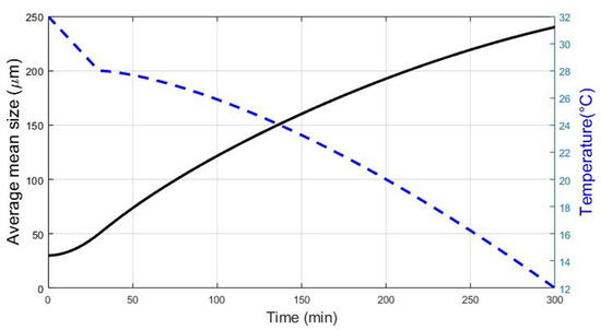
Figure 1.
Desired mean size profile (black) and corresponding temperature profile (blue, dashed).
In order to further apply and study the different RBF control approaches, the crystallization model needs to be evaluated relative to the degree of accuracy from the possible inputs to the RBF model with the outputs of the same RBF/crystallization model. This was conducted by taking a subset of data (training data) from the simulated case and comparing/analyzing with the predictions from the RBF model. The training data size was then increased and the process was repeated until the training data was the same (identical) as the validation data.
For analysis of the RBF performance, the coefficient of determination (), mean squared error (MSE) and the general cross validation () [29,37] statistics were used (Equations (26) and (27)).
where is the number of RBF nodes, and is a penalization factor. The has been adopted from the work of Friedman et al., 1991 [37], and it assumes the value of 3 for the RBF validation. These evaluations are performed for a series of different transfer functions, which are described previously in Section 2.2, using the toolbox developed by Jêkabsons [38].
For training data, the desired output was the mean crystal size through the characteristic length dimension. This variable was considered valid as it can be measured online through different sensors and measurement techniques such as the FBRM technique and Particle View Microscopy (PVM). As for the input data to train the RBF model, temperature and current simulation time were set as the main information. Both input data can be easily tracked and measured online. The concentration of the dissolved API could be a plausible choice as well, as its measurement and online values could be deducted from a series of methods, namely the application of Ultraviolet–Visible (UV/Vis) spectroscopy or Attenuated Total Reflectance Fourier Transform Infrared (ATR-FTIR) spectroscopy. While certainly the presented methodology can work with many diverse inputs, in this work we focused on simple measurements typically available in industrial pharmaceutical manufacturing (which are typically low). Moreover, solute concentration within the medium is directly correlated to the system temperature and crystal seed/crystals present. The implication of this correlation resulting from only one driving force for the crystal growth (supersaturation) would imply an increased risk of both unfeasible RBF models of even the need to increase the depth of the hidden layers. That approach is out of the scope of this work. The data input for the RBF networks assumes then the form of:
with representing the process inputs, and representing the process outputs.
2.4. RBF Strategies for Crystallization Processes
The availability of the process data is of utmost concern for the implementation of the different RBF-based strategies for the control of the crystallization process. Three strategies for the training of the RBF model were proposed, that target the absence of previous data, limitations in the number of possible/feasible readings from the online process and the existence of previous data. They are presented as, respectively, Growing Window methodology, Moving Window methodology and Golden Batch methodology.
2.4.1. Growing Window Methodology
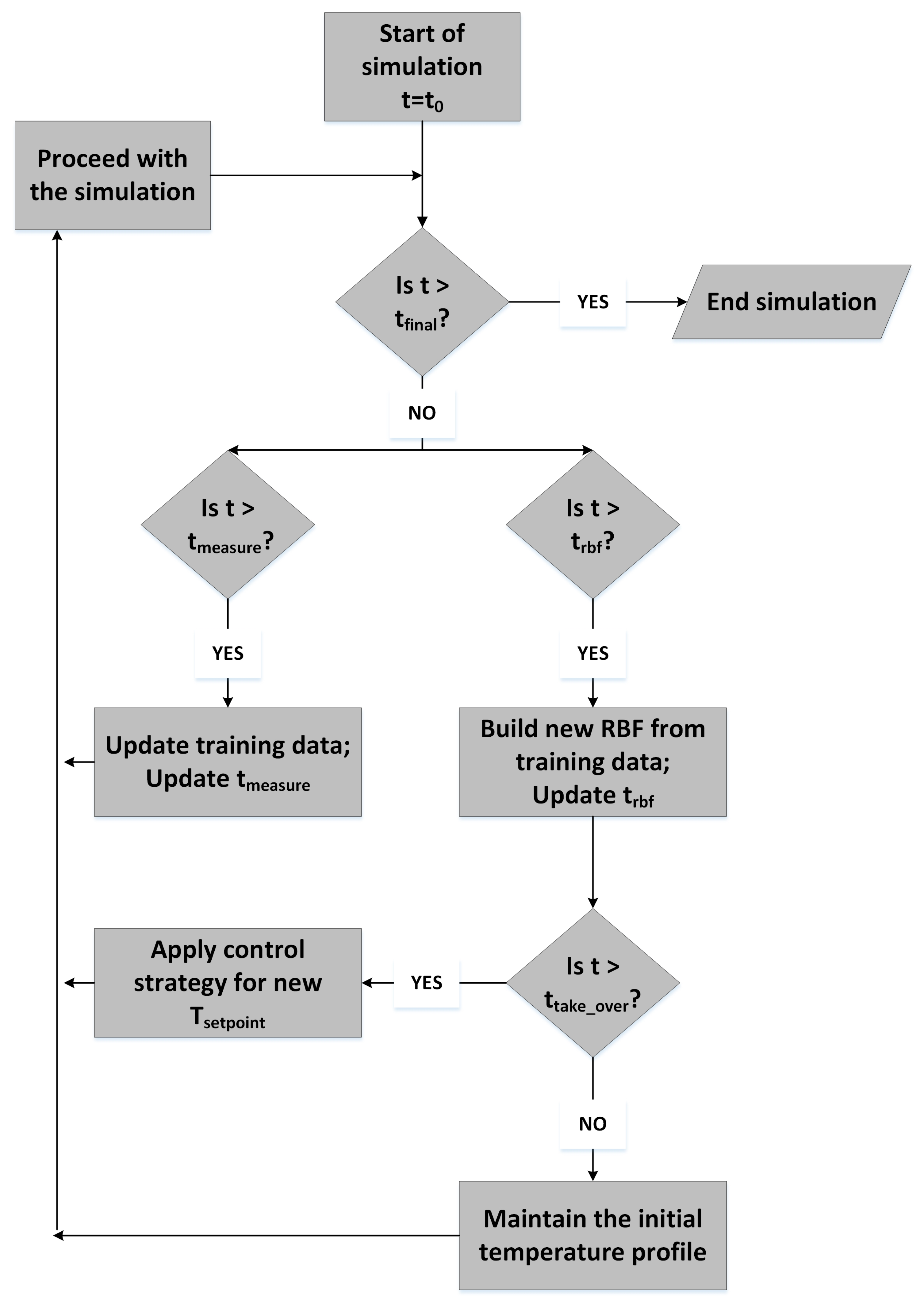
The Growing Window (GW) methodology is proposed for case scenarios where no data are available previous to the experiment or the simulation case. No limitations on the amount of data used for the RBF construction exist, leading to a constant growing of the training set for the system. Four major time points within the simulation/experimental setup require prior understanding, in order to provide accurate results and system behavior from the RBF itself. These key points are:
- Measurement time (): This represents the time of the experiment or simulation in which new data are available for the process variables being measured and/or tracked. For this work, mean crystal size, time and temperature are the measured variables. Depending on each system, different sensors might have different sampling times, which lead to the highest of these measuring times being defined as the highest amongst the measured process variables. Once this value is achieved, the upcoming measurement time is updated to the system, until the experiment/simulation is finished.
- Take over time (): This represents the time at which the RBF control takes over the initial system. Due to the fact that no initial historical data are available, the RBF model has no training data to provide a feasible solution or even a solution at all. Therefore, there is the need to allow the system to initially collect enough data until the RBF is suitable to take over and assume the temperature setpoint control.
- RBF build time (): This represents the time series in which a new RBF model is built from the training data available. The initial value for the coincides with the , and once it is reached, a new value is updated to the system until the experiment/simulation is finished.
- End of experiment (): This represents the end of the experiment/simulation, defining how many RBF implementations have been used and how much data has been collected.
Figure 2 shows the workflow of the Growing Window methodology:

Figure 2.
Workflow used to apply the radial basis functions (RBF) Growing Window methodology to crystallization.
2.4.2. Moving Window Methodology
The Moving Window (MW) methodology is proposed for case scenarios where there are limitations in the amount of data that can be collected or stored online, in contrast with the Growing Window approach. To this end, training data are replaced in a chronological order, where the oldest collected data points are replaced with the most recent ones. The size of the training data is kept constant once the maximum size is achieved. A new key point is introduced to this methodology:
- Maximum data size (): this represents the maximum length of the training data stored for RBF assembly, within a n × m matrix (n representing the different inputs, and m the input observations).
The workflow of the Moving Window methodology is shown in Figure S2 in the Supplementary Material.
2.4.3. Golden Batch Methodology
The Golden Batch methodology is applied in industry [20], where historic data from a successful experiment/operation are available and are used to either take full control of the new batch operation or to guide the process in its early stages of simulation/experimentation. The latter approach one was applied within this work, where the initial set of data (‘golden data’, from the ibuprofen case scenario) is used to assemble the first RBF models. As soon as new measurements are being collected, the initial training data are being replaced, in order to replicate and understand the disturbances and uncertainties of the process when compared with the Golden Batch data. Figure S3 in the Supplementary Material shows the workflow of the Golden Batch methodology.
2.5. RBF Soft Sensor and Predictive Control
Two approaches for the application of the RBF control methods were used: (i) using the RBF as soft sensor to estimate the upcoming/future deviation between the desired mean size (trajectory) and the estimated mean crystal size, and (ii) as a predictive control in order to minimize the deviation between the simulation/experimental results and the desired mean crystal size as a kind of nonlinear model predictive control.
2.5.1. RBF Soft Sensor
The objective of the RBF soft sensor was to monitor the measured RBF input and output state variables from the ibuprofen crystallization process (temperature and mean crystal size). The course of the crystal growth pattern was forecasted by the soft sensor. The soft sensor output was then used to calculate the future deviation from the desired target size () (Equation (29)). This deviation was then applied to a PI controller as an error measurement with the updated time of every three minutes (crystal growth pattern were re-predicted by the soft sensor every three minutes), but applied at the current time (Equation (30)). The PI controller applies then changes to the setpoint of the cooling water. The cooling system was assumed perfect, and therefore the water temperature changes were instantaneous (no system dynamics assumed).
It was assumed that the system had a delay of three minutes, in order to replicate the time required to save, convert and analyze the measurement data in real-time.
2.5.2. RBF Predictive Control
The objective of the RBF predictive control approach was to optimize the cooling water temperature setpoint over a future horizon, in order to minimize the deviation within the same period. The optimization problem was based on the work developed by Seborg et al. 2004 [16], and is described by Equation (31).
where y(k) is the output of the RBF model at time step k, u(k) are the inputs of the RBF model at time step k; and are weighting coefficients for the optimization function, P is the prediction horizon, C stands for the controlled horizon, and are the maximum allowed values for the optimized inputs; is the time step change between measurements, and and stand for the maximum change between optimized future predictions.
For the application of the RBF predictive control, it was assumed that the cooling/heating rate is saturated at the value of 0.5 C per minute, as an a priori knowledge of crystallization processes. This also avoids the spontaneous occurrence of secondary and primary nucleation, while the RBF is being updated with more process data. As the RBF model was predicting the outputs over P periods, the predictions were being extrapolated further away from the confidence range of its training data. Therefore, the controlled horizon was set to 1, in accordance with available literature [16]. The setpoint transition between current and the optimized value was smoothed through the current difference between the real-time temperature in the crystallizer and the predicted setpoint temperature, as shown in Equation (32).
For the optimization problem, the Matlab function fmincon was used to find the optimal answer, with initial guesses for P predicted values being assumed the same as the corresponding temperature at time k,k + 1,…,k + P−1.
2.6. Case Study Application
Both approaches presented in this study were evaluated within Monte Carlo method. For each control application (soft sensor and predictive control), and for each RBF methodology (Growing Window, Moving Window and Golden Batch), one simulation was performed where no disturbances or uncertainty were included: Following this step, one disturbance at a time was applied, with the half of the uncertainty range specified on the main kinetic parameters; and , initial seed mass, water content of ethanol solvent as listed in Table 1:

Table 1.
Disturbances applied in the control applications and their uncertainty range.
For this step, the RBF strategies were also compared with a traditional PI controller regime, where the error was directly fed to a PI (with the same tuning as the RBF PI controller). Lastly, a sampling space of 300 samples magnitude was created within the uncertainty space presented in Table 1, for the same process variables and parameters. The behavior of the controlled applications and open-loop scenarios were analyzed and compared amongst themselves using the integral of the absolute error (IAE) and a weighted IAE () (Equations (33) and (34)) for the single-step disturbances and analyzing the cumulative distribution function for the Monte Carlo simulations.
3. Results
3.1. RBF Validation
The initial available data for the analysis of the RBF networks are composed of a set of 301 points of temperature and mean crystal size values over a period of hours, linearly distributed (once every minute plus the initial conditions of the crystallization). The initial size of the training data corresponds to 51 points (up to 50 min in the crystallization), and every new set of training data has an additional 5 data points. For the 5 different RBF transfer functions applied, the Biharmonic and Multiquadratic functions showed similar results regarding the prediction and data fitting. The same behavior was observed between the Inverse Multiquadratic function and the Gaussian transfer function (corresponding Figure S4 can be found in the Supplementary Material). The Thin Plate Spline transfer function displayed an irregular behavior: despite achieving a higher coefficient of determination first, the irregular sudden decrease of its stabilization indicated that certain sets of data do not provide accurate predictions from the same transfer function nodes for the ibuprofen crystallization. The cross-validation score achieved its peak at around 60% of having the full set of training data, which corresponds to a better MSE score of the Thin Plate Spline transfer function, followed by the Biharmonic and the Multiquadratic function.
For testing the robustness of the different transfer functions architecture, random linear noise was introduced within the training data, for 100 samples with the Latin Hypercube Sampling (LHS) method [39]. The noise addition was limited to maximum change for temperature and maximum deviations of in time measurements.
The Thin Plate Spline transfer function achieved the best answer pattern to the irregular input data, with residuals reaching a maximum of 2.4 m, and an average MSE of 0.489 m. On the other hand, the Inverse Multiquadratic and Gaussian functions presented the worst performance, namely within the first time period of the crystallization. Residuals could achieve deviations of above 40 m, and despite the late tendency to track on pair with the validation data, the average of the MSE was within a magnitude of 79 m. The figure showing the output space for the different RBF transfers functions while seeding noise within its training data, and also the residual/deviation plotting from the target mean size for each respective RBF as well as the scores for highest and average MSE and lowest and average can be found in Figure S5 and Table S1, respectively in the Supplementary Material.
Despite the better overall results from Thin Plate Spline transfer functions, the instability of the scores for high training data values prohibited further usage of this transfer function. With this in mind, the Multiquadratic transfer function was chosen to apply for the control strategies proposed in Section 2.4.
3.2. RBF Soft Sensor Application
The soft sensor approach was applied to three presented methodologies. Initial simulations were presented for open-loop scenarios, where the initial crystallization conditions (, , ) were set to their value specified in Table 1, and the process parameters (, ) were assumed to be their reported literature value. Following the initial simulation, uncertainty was included, disturbing one process parameter/initial condition at a time, with half the value of both the upper bound and lower bound of the confidence interval. The last scenario was performed with Monte Carlo inputs. Assumptions and conditions for the RBF soft sensor application are presented in Table 2.

Table 2.
Assumptions and conditions of the crystallization for the RBF soft sensor and predictive control applications.
3.2.1. Moving Window Soft Sensor Application
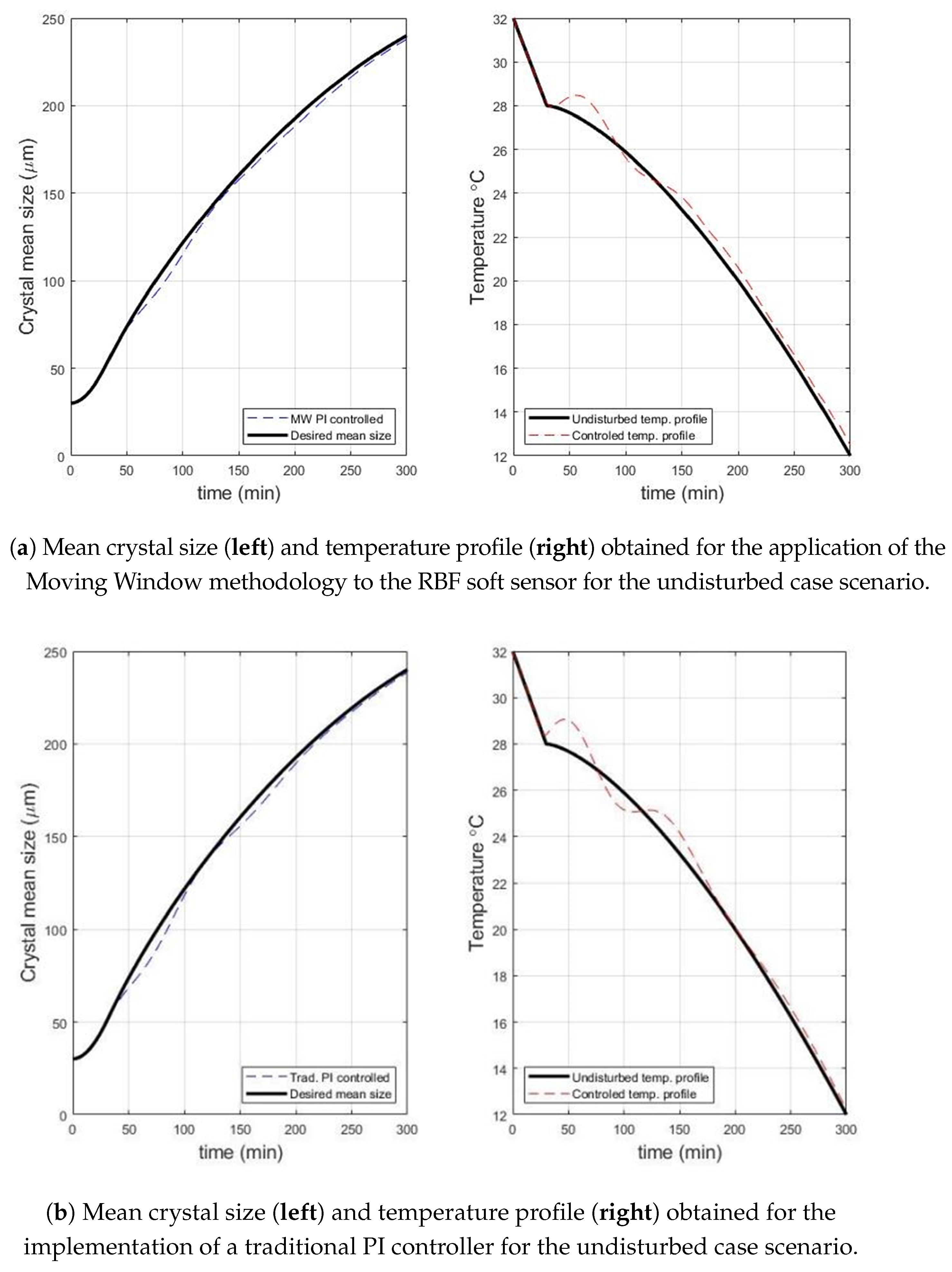
Figure 3a shows the behavior of the RBF soft sensor with the Moving Window methodology, for an undisturbed case scenario. The transition from the initial temperature profile (at 30 min) to the PI profile was accompanied with a small misjudgement of the necessary temperature input for the next 3 min period. This caused the mean crystal size to deviate from its expected course, as seen in Figure 3a, at 60 min. There was therefore a period of increased error, in which the RBF needed to collect data to correct the misstep taken. This was, however, achieved over the course of the whole experiment, and the final deviation from the desired mean size was lower than 2 m.
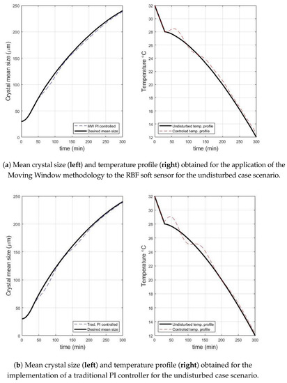
Figure 3.
Comparison of undisturbed and disturbed case scenarios for the application of the Moving Window methodology to the RBF soft sensor and a traditional PI controller.
For the same scenarios with no disturbance applied, Figure 3b shows both the mean size trajectory achieved by the traditional PI controlled scenario, and the respective temperature profile. The PI only started operating at 30 min of simulation time, in order to have a fair comparison with the RBF PI case. Similarly to the RBF PI soft sensor, using the Moving Window methodology, the traditional controller had an early off-set deviation, due to the change in the temperature behavior when compared with the undisturbed temperature profile. This off-set was then corrected through the course of the simulation. The metric evaluation performed for both cases can be found in Table S2 in the Supplementary Material.
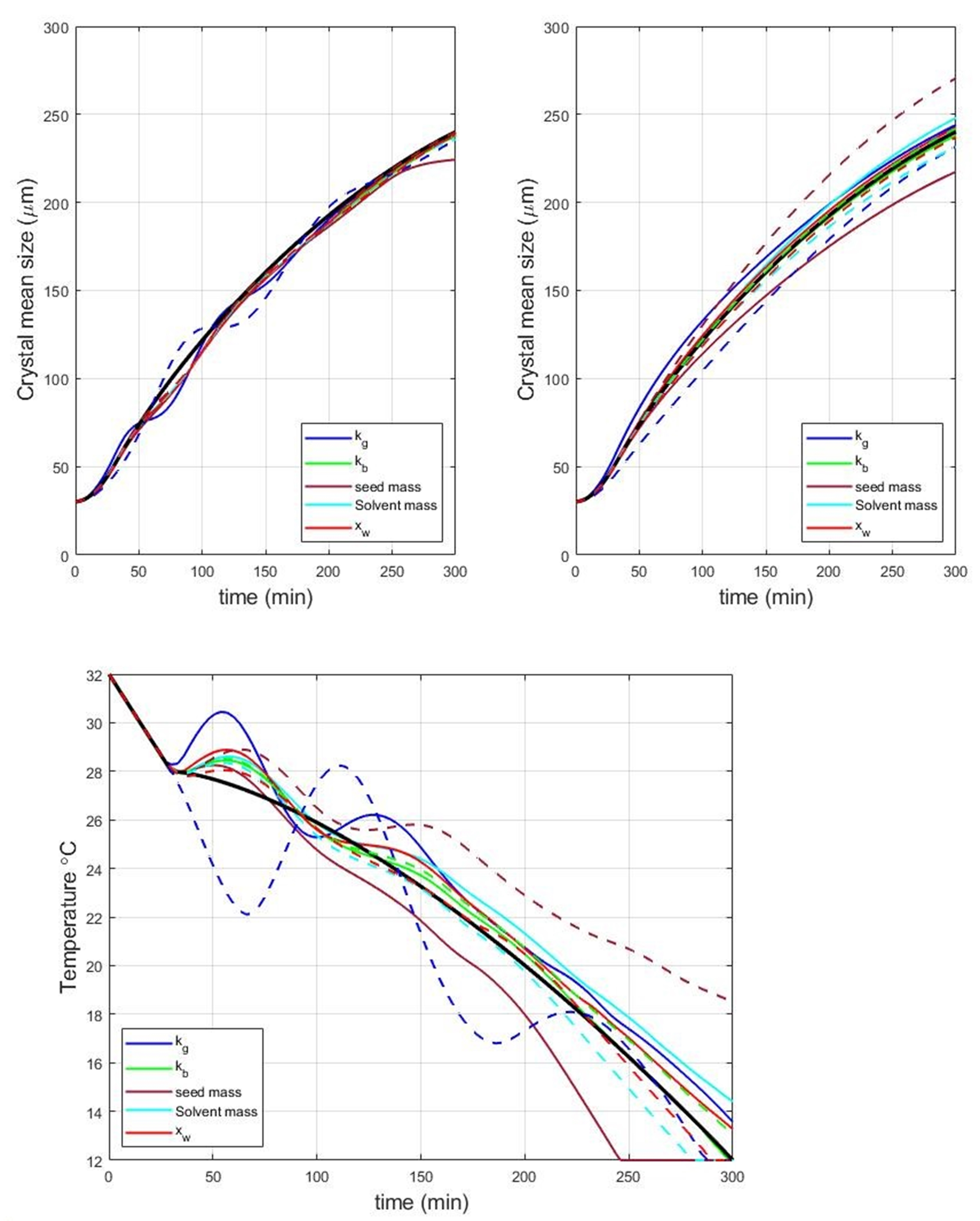
The individual disturbances propagated through the system are shown in Figure 4 (top) for both closed-loop and open-loop scenarios. As demonstrated, the mean crystal size was achieved for the disturbances implemented. The only exception to this performance was for positive disturbances in the initial seed mass (more initial crystal mass present at the beginning of the process). However, as the crystallization process was designed to achieve almost no supersaturation at the end of the experiment, increments in the seed will reduce the overall size of the whole crystal population, as there was not enough dissolved API in the crystallizer to achieve the desired size set for an undisturbed run. This was, therefore, an impossible task to achieve. Nonetheless, as it was observable in Figure 4 (bottom), the PI controller showed that the behavior for this case was correct, as it manipulated the temperature to reduce it as far as possible. It was, however, saturated at 12 C.
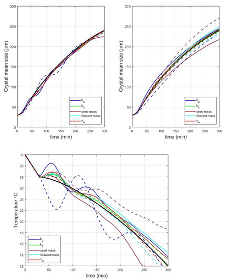
Figure 4.
Controlled mean crystal size (top-left), open-loop mean crystal size (top-right) and controlled temperature profile (middle) in the presence of and obtained for the application of the Moving Window methodology to the RBF soft sensor with single step disturbances (positive disturbance: full line; negative disturbance: dashed line).
As for the behavior shown for negative changes in , the initial offset that the RBF soft sensor received at the time at which it took full control of the system, transformed its answer into a temperature decrease order. This caused the system to overreact and for a brief period of the crystallization (between 100 and 150 min), the mean crystal size was above the desired target. Due to the system dynamics, the temperature rise rate was delayed, as the RBF was renewing its training data. During this period, however, dissolution was occurring, causing the mean crystal size to drop below the desired target. This cycle repeated one more time before stabilization occurs, achieving a mean crystal size that was within the expected margin (235 m final size).
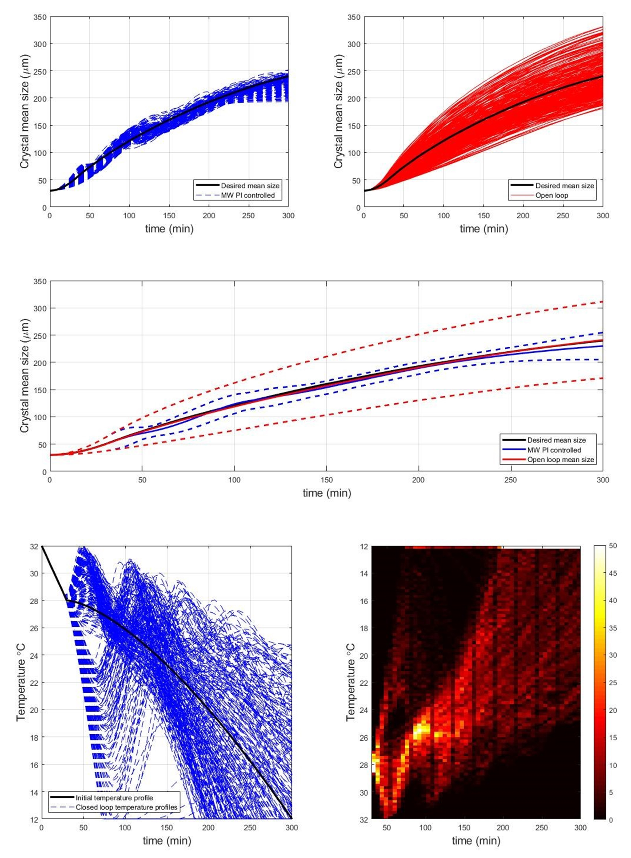
The results from the Monte Carlo simulation, in which case all disturbances were sampled from their uncertainty range and perturbed simultaneously, for the Moving Window PI soft sensor are presented in Figure 5. Both closed-loop and open-loop cases are presented, together with the average and the 95% confidence interval for the obtained results.

Figure 5.
Controlled mean crystal size (upper left corner), open-loop mean crystal size (upper right corner), confidence interval of controlled and open-loop cases (middle) and corresponding controlled temperature profiles (bottom-left) and heat map of the temperature profiles (bottom-right) over the course of the simulations obtained for the application of the Moving Window methodology to the RBF soft sensor with Monte Carlo sampling disturbances (300 Latin Hypercube Sampling (LHS) samples simulated [39]).
The obtained results show that for the majority of the input uncertainty the outcome final mean size was restricted to an interval of 50 m (between 200 m and 250 m), with an average mean particle size of 229 m. Due to the fact that the temperature of the system was being manipulated by the RBF, within certain conditions met and within the imposed uncertainty, two phenomena occurred that can be non-existent to the open-loop cases:
- The sudden drops in temperature (Figure 5) pushed the system to the secondary nucleation regime, creating a surge of new and small crystals that reduced the overall mean particle size. This increment of the number of small crystals also reduced the potential of achieving the target size, as it can be compared to the impact of having increased number of seed crystals in the system (however, this time they appeared during process operation, instead of being present from the beginning);
- Increments in the temperature above the predefined setpoint can create conditions for the system to become undersaturated, reducing the overall mean size. However, small crystals will be dissolved due to dissolution mechanics, and the overall solute concentration increases. Therefore, with fewer particles within the system and more solute, the overall dynamics of the system have changed, and the RBF required more time to adapt, leading to wrong predictions.
3.2.2. Growing Window Soft Sensor Application
Similar to the steps performed previously in the Moving Window methodology, the RBF soft sensor with the Growing Window methodology was firstly studied for an undisturbed case scenario. The figure showing the behavior of the RBF soft sensor with the Growing Window methodology, for the undisturbed case scenario can be found in Figure S6 in the Supplementary Material. The mean size prediction error after the transition period was expected to occur, just as it was reported with the Moving Window soft controller. Both methodologies had the same training data for the undisturbed case. The continuous addition of training data (measurements) without imposing an upper limit did not mislead the Growing Window RBF about learning the system dynamics. The deviation on the final mean size was less than 3 m, showing a slightly bigger offset than the Moving Window methodology.
The individual disturbances propagated through the system are shown in Figure 6a for both Growing Window soft sensor closed-loop and open-loop scenarios. The controlled system behaved similarly to the Moving Window methodology when the latter was analyzed for individual step changes. The main visible difference was within the response for a negative disturbance in the crystal kinetic. The offset from the desired mean size was reduced after 150 min, when compared with the Moving Window methodology. The final deviation from the target mean size is 4 m, (236 m, final size), a one unit improvement compared with the previous methodology. The controlled temperatures profile can be found in Figure S7 in the Supplementary Material.
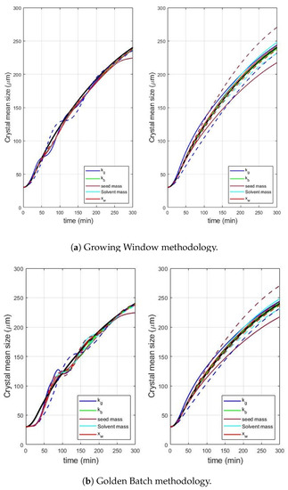
Figure 6.
Controlled mean crystal size (left) and open-loop mean crystal size (right) obtained for the application of the different methodologies to the RBF predictive soft sensor with single step disturbances (positive disturbance: full line; negative disturbance: dashed line).
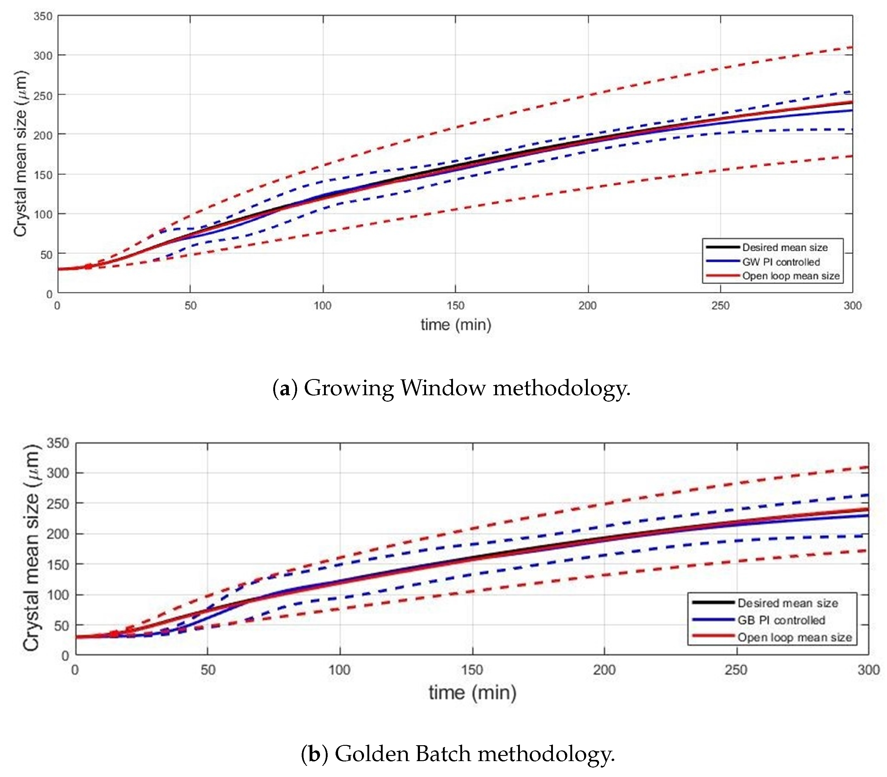
The results from the Monte Carlo simulation for the Growing Window PI soft sensor are presented in Figure 7a, for both closed-loop and open-loop cases, together with the average and the 95% confidence interval for the obtained results.
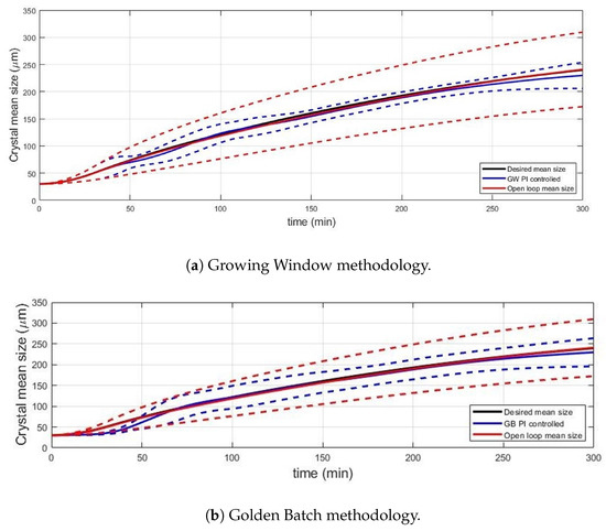
Figure 7.
95% confidence interval of controlled and open-loop cases obtained for the application of the different methodologies to the RBF soft sensor with Monte Carlo sampling disturbances (300 LHS samples simulated).
Similar to the Moving Window soft control, the majority of the results were restricted to an interval of 50 m, with an average mean size of 230 m. The improvement on the mean average is explained by the higher number of available training data for the RBF. If the crystallization achieves the dissolution or secondary nucleation threshold more than once, the RBF is now better adapted to the changes within the system dynamics. However, for a total crystallization time of 5 h, the possibility of occurrence of both these events is minimal, even with temperature changes in the order of 15 C within 30 min (double the amount allowed for the predictive control approach), which can be found in Figure S8 in the Supplementary Material.
3.2.3. Golden Batch Soft Sensor Application
A figure showing the behavior of the RBF soft sensor with the Golden Batch methodology, for an undisturbed case scenario, can be also found in the Supplementary Material (Figure S9). As it is provided with initial data prior to the crystallization process, the Golden Batch RBF PI took control of the system from its starting point. However, the Golden Batch PI soft sensor failed to replicate the temperature trajectory of the main case for the initial time period. The temperature profile did not decrease, and as a consequence, the mean size of the crystal did not evolve. Consequently, the mean crystal size had a negative offset for the first 50 min of the operation. From here, the RBF soft sensor inverted the system behavior, to counter the overcooling that was initially provided to the system. It can be observed that the mean size had a positive off-set between 60 and 100 min of operation. At roughly 135 min of simulation, the RBF PI had an abrupt change of behavior, and instructed the system to start heating instead. Paying close attention to the mean crystal size profile, this time step corresponds to the rate change of the crystal growth pattern (blue dashed line, in Figure S9 in the Supplementary Material).
The traditional PI controller, which was active since the beginning of the simulation (Figure S10 in the Supplementary Material), showed similar behavior to the Golden Batch methodology. The system started with an off-set regarding the mean size, due to the different cooling patterns used for the main case scenario. The mean size trajectory achieved by this controller was similar to the results obtained from the RBF Golden Batch. However, as the Golden batch was predicting into the future step, stability and closer results to the desired mean size were achieved faster with the RBF methodology.
The individual disturbances propagated through the system were shown in Figure 6 for both Golden Batch soft sensor closed-loop and open-loop scenarios. The main difference regarding this methodology compared with the previous cases was that the negative disturbance propagated through the growth kinetic was countered in less time than any of the previous methodologies (Figure S11 in the Supplementary Material). This was due to the fact that the PI was active from the very beginning of the simulation, having more time to actuate on the predicted offset. Additionally, the replacement of the initial training data with online measurements slowly replaced the ill-conditioned data, as it did not represent the current system anymore. However, until it was fully or significantly replaced, the PI could still perform an action based on the initial training data. Despite not being able to truly replicate the system dynamics, the off-set gain caused by such action was still positive, slowly tending towards the desired setpoint. When compared with both Growing and Moving Window, the final deviation from the target mean size is 1.5 m, (238.5 m, final size), the best achievement for one-step changes amongst the PI strategies. The temperature profiles for the individual disturbances can be found in Figure S12 in the Supplementary Material.
The results from the Monte Carlo simulation for the Growing Window PI soft sensor are presented in Figure 7b, for both closed-loop and open-loop cases, together with the average and the 95% confidence interval for the obtained results. The Monte Carlo temperature profiles and temperature heat maps are provided in Figure S13 in the Supplementary Material. For the presented case scenario, the overall crystal final mean size was similar to the results obtained by the previous RBF methodologies. There are, however, high off-sets for the mean crystal size during the simulation, with special emphasis halfway through the crystallization process. At this period of time, half of the initial training data were still in use by the RBF. The two sets of data (initial and process collected) could have different impact in the RBF predictions itself, with said difference being noticed on the behavior of the predicted error. It was at mid simulation time that both sets of data presented a high disparity between the nodes weight attribution leading to huge deviations in the error prediction. Nonetheless, the end crystal size variation was within the order of 50 m, and the average mean size is 230 m.
3.2.4. Control Performance Evaluation for RBF Soft Sensor Methodologies
The integral of the absolute error and the weighted integral of the absolute error for the different PI soft sensor applications are presented in Table 3. The results showed that the RBF soft sensor has better performance in tracking the desired mean size over the course of the simulation. With the exception of negative disturbances in for all the methodologies, the IAE metric was below the result achieved by the traditional PI controller. However, despite the overall deviation being lower, if the final size was considered to be more important than the ongoing mean particle size, the performance of the PI soft sensors was considerably worse (Golden Batch being the exception). In particular, the Growing Window methodology for the PI soft sensor was not able to outrank the traditional PI controller in any of all presented cases, noting that the deviation from the trajectory mean size was considerably higher at later time periods when compared with the traditional PI controller or the Moving Window methodology.

Table 3.
Integral of the absolute error (IAE) and evaluation for the single step disturbances in the different RBF strategies.
As for the Golden Batch application, the availability of the initial training data from the process since the beginning of the operation was able to give the advantage point to the controlled system. Even if the predictions were not correct, the replacement of previously existing data with more recent and accurate data guides the crystallization towards stability and success. The final mean sizes achieved by both strategies are presented in Table S3 in the Supplementary Material. The final mean size, confidence interval and the probability distribution for the Monte Carlo simulations applied to the RBF soft sensor in comparison with open-loop (OP) results, are presented in Table 4.

Table 4.
Final results for the Monte Carlo RBF PI soft sensor and predictive control simulations.
For the Monte Carlo simulations, the majority of the final crystal size values were below the desired target, as can be observed by the average mean size obtained in all the simulations. Nonetheless, the RBF PI soft control was able to achieve the gap interval assumed for this scenario (less than 10 m away from the 240 m target) for more than of the simulations. If this interval was relaxed to a gap of 20 m, more than of the runs reached an acceptable mean size target. Taking the example of the Moving Window methodology, it was possible to observe that the controlled system did not achieve any oversized crystal, that is, with a size bigger than 260 m. Control-wise, this is a positive outcome when compared with the opposite case, where the crystal is mostly oversized. It is easier, from a crystallization perspective, to cool down a bit further the process batch to achieve the desired size, than it is to heat and risk losing part of the smaller population. The cumulative distributions for the Mowing Window, Growing Window and the Golden Batch methodologies are reported in Figures S14–S16, respectively in the Supplementary Material.
3.3. RBF Predictive Control
The predictive control approach was applied to three presented methodologies similar to the soft sensor application. Initial simulations were presented for undisturbed case scenarios, where the initial crystallization conditions (, , ) were set to their specified value in Table 1, and the process parameters (, ) were assumed to be the reported literature values. Following the initial simulation, uncertainty was included, disturbing one process parameter/initial condition at a time, with half the value of both the upper bound and lower bound of the confidence interval reported in Table 1. The last scenario was performed with Monte Carlo inputs, where 300 samples were generated using LHS [39], from their respective input ranges for disturbances and simulation. In this way, disturbances impact on the quality product attribute were evaluated simultaneously and presented a more comprehensible metric evaluation of the candidate control strategies. The same simulation conditions from the soft sensor approach were used for the predictive mode, with one exception:
- In order to provide the RBF with enough significant training data, the predictive control only took control after 1 h. Following the linear decrease of temperature from 32 C to 28 C, there was a linear increase of the temperature from 28 C to 30 C. This provided more training data regarding the effect of heating on the crystallization, and if the correct conditions were met, the RBF could adapt to dissolution occurrences. RBF predictive control using Golden Batch did not follow this pattern and instead took control over the cooling system from the very beginning of the simulation.
The conditions of the RBF predictive control can be found in Table 2.
3.3.1. Moving Window Predictive Control
The figure showing the behavior of the RBF predictive control with the Moving Window methodology for an undisturbed case scenario can be found in Figure S17a in the Supplementary Material. There was a transition from the initial temperature profile (at 30 min) to a 30 min heating period, in order to provide enough training data to the system to understand the dynamics related to the system temperature increase. Once this heating period has finished, the predictive control took 12 min of shifting heating/cooling actions, until an almost linear cooling profile was decided for the rest of the simulation. For three times, the predictive control had to perform a halt on the cooling rate to adjust the mean size profile, but it did achieve the desired target nonetheless. It was worth noting that despite the fact that the system was not disturbed by any of the uncertain parameters, it started with an offset due to the new initial temperature profile. The simulation results of the one process parameter/initial condition disturbance at a time can be found in Figures S18 and S19 in the Supplementary Material).
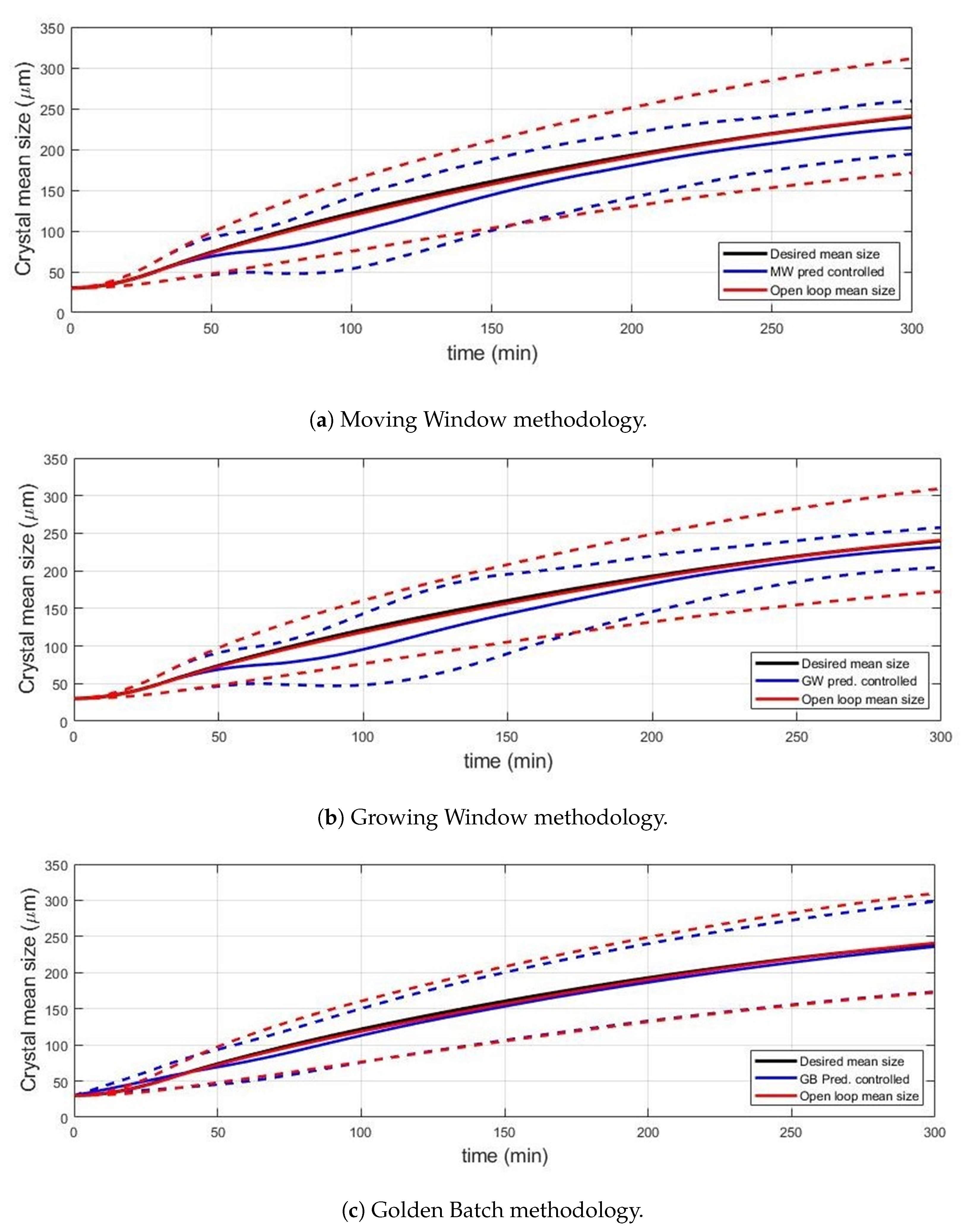
The results from the Monte Carlo simulations for the RBF Moving Window predictive control, together with the average and the 95% confidence interval are presented in Figure 8a. The results showed a tendency to underpredict the upcoming mean crystal size, leading to an average mean size of 226.8 m, roughly 13 units below the desired target. On the other hand, there were relatively few cases of overgrown crystals, indicating that the heating rate dynamics have been well captured by the radial basis functions, as shown in Figure 8a, for the period of 200 to 250 min. During this period, a few overgrown simulations were plummeted with a temperature rise, leading to a smaller end deviation. The temperature profiles and temperature heat map for the Monte Carlo simulation with Moving Window predictive control are presented in Figure S20 in the Supplementary Material.
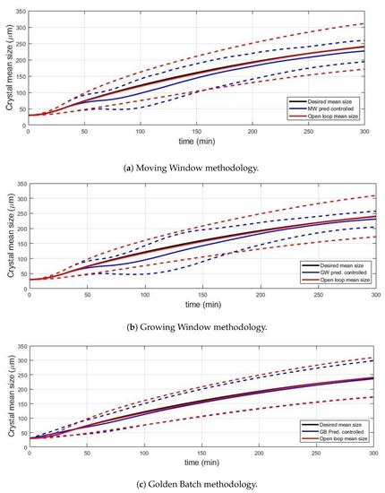
Figure 8.
95% confidence interval of controlled and open-loop cases obtained for the application of the different methodologies to the RBF predictive control with Monte Carlo sampling disturbances (300 LHS samples simulated).
3.3.2. Growing Window Predictive Control
The figure showing the undisturbed case scenario for the RBF Growing Window predictive control is presented in Figure S17b in the Supplementary Material. In contrast with the Moving Window methodology, the Growing window did not lose any of its initial training data. The initial behavior was the same as the Moving Window methodology, due to the fact that both have the same training data. From the 75 min period, the training data for the RBF was in this case different, and due to the influence of the early points of the system (where the growth rate was slower), the control produced an overshoot behavior. This deviation was then corrected over the course of the simulation. This however confirms that the different methodologies have been predicting differently. The simulation results of the one process parameter/initial condition disturbance at a time can be found in Figures S21 and S22 in the Supplementary Material.
The results from the Monte Carlo simulations for the RBF Growing Window predictive control are presented in Figure 8b, for both closed-loop and open-loop cases, together with the average and the 95% confidence interval for the obtained results. As with the Growing Window methodology, the average mean size was below the target objective, achieving however better results than the previous method: an average mean size of 231.1 m, which was still within the acceptable range. The main difference between both methodologies was the acting time for the early off-spec cases (time 130–150 min). Where a set of simulations was overshooting the desired mean size. The Growing Window methodology still kept the first hour of training data, as opposed to the Moving Window, which changed the future temperature output to cool as fast as it was allowed. The same behavior was achieved by the Moving Window, however these deviations only took place in a different period of time. The respective Monte Carlo temperature profiles and heat map are provided in Figure S23 in the Supplementary Material.
3.3.3. Golden Batch Predictive Control
The figure showing the undisturbed case scenario for the RBF Golden Batch predictive control was presented in Figure S17c in the Supplementary Material. Differently from previous methodologies for predictive control, the Golden Batch predictive control did not have an initial change in the temperature profile, starting the simulation at 32 C, and having absolute control of the future temperature setpoints from the start of the operation. There are two main behaviors to be noticed in the results:
- For early process times, the Golden Batch was unstable, not being able to find a smooth pattern to follow. This causes an off-set between the desired and the current mean crystal size.
- Once the unstable period has passed, the future predictions tend towards the initial training data temperature at the respective time. This indicated that the initial set of data (the Golden Batch data) was overruling the weight of the newly incorporated measurements. As there was no disturbance included, the final mean size shows almost no deviation.
The simulation results of the one process parameter/initial condition disturbance at a time can be found in Figures S24 and S25 in the Supplementary Material). These two behaviors were also seen in these disturbed systems. The initial unstable cooling/heating pattern was followed by the overruling of the fresh new data, leading towards the same temperature profile as the initial training set. Moreover, as the new data collected were dependent on the future predictions of the RBF (which lead to the new temperature and mean size measurements), the fresh data could be “poisoned”, leading the system towards an irreversible point where there was not sufficiently rich information regarding the initial system dynamics. This effect is shown through the Monte Carlo simulations for Golden Batch predictive control and their respective temperature profile. This is presented in Figure 8c and in Figure S26 in the Supplementary Material, respectively.
With little exception, the RBF predictive control employing a Golden Batch methodology led the system towards the initial temperature profile. This caused the system to have almost no changes regarding the open-loop scenario, where the initial temperature profile was already employed. The impact of the fresh provided data was overrun by the early data, and by the time it was worth more than half of the total initial data, the system was already in a point of no return, turning most case scenarios into uncontrollable cases.
3.4. Control Performance Evaluation for Predictive RBF Methodologies
The integral of the absolute error and the weighted integral of the absolute error for the predictive control applications are presented in Table 3. The results show that the Moving Window methodology is best suited to deal with uncertainty in parameters/process variables that have a bigger impact in the system such as growth kinetics and seed deviations. For smaller impact disturbances, the Moving Window has a smoother approach, leading to a lower sum of errors in the end, but still achieving a lower score regarding the average mean size at the end of the simulation (Related data can be found in Table S4 in the Supplementary Material). The Golden Batch methodology has the advantage of controlling the system from the very beginning, and being relatively independent from the continuous data that it is provided.
The final mean size, confidence interval and the probability distribution function for the Monte Carlo simulations applied to the RBF soft sensor are presented in Table 4. The figure showing the cumulative distribution function of all three RBF predictive control methodologies can be found in Figures S27–S29 in the Supplementary Material. For the Monte Carlo simulations, like the PI soft sensor methodologies, the final crystal size was below the desired target, as can be observed by the average mean size obtained in all the simulations. The RBF Golden Batch did not provide accurate and reliable control action for huge disturbances, and a thorough analysis of the available training data is recommended for the implementation of such a strategy. Despite that, the performance of the RBF Growing Window methodology outranks the other methods, as it achieved in almost 66% of the simulated cases with an average mean size within the desired gap interval. This outperforms even the PI soft sensor methodology, and even further if considered that the Growing Window RBF predictive control only was active for 4/5 of the process. Improvements to the performance are expected if the Growing Window methodology is applied with extra initial data, in order to control the system from the very beginning.
4. Conclusions
RBF PI soft sensor control and RBF predictive control show promising potential for the control of a crystallization process. In both scenarios, the step changes have been stabilized within the time range of the process, with Moving Window and Golden Batch presenting the best results for an RBF PI soft sensor, and the Growing Window outperforming the remaining methodologies for predictive control. For all cases, the RBF construction was performed under 0.1s for the maximum allowed data (3 data points per minute), and the optimization problem was solved under 10 s. This should, however, be taken into consideration for the increase on the data matrix for larger data quantities, such as second-based measurements in real-time. The time delay for the RBF construction and possible optimization might have to be included for tuning purposes. Despite the better performance of some methodologies over others in the different applications proposed, the choice of which methodology and approach to choose relies mostly on two elements. Data availability and quality and expected deviations from the system:
- The data availability is of utmost importance for the choice of a Golden Batch methodology. Not only the availability of data is required, but the reliability of its annals is demanded. If only a segment of a certain process is used for the initial training data of a Golden Batch RBF is used, the predictions for the non-included process behavior should not be trusted. This was verified for the predictive control using the Golden Batch methodology, where there was not sufficient information to decide on which action to take, even when knowing that there would be a deviation. The reason why the PI soft sensor accomplished good results for the same methodology, is because the controller action was not entitled to the RBF itself, but to the PI controller. Regarding quality, for all the methodologies, the RBF is being trained with the data it is provided with. If accurate data is not given to the model, the learning process is hampered, and the predictions of this referred model cannot be trusted.
- The expected deviations to the system refer to known deviations, expected deviations or lack of knowledge of the system dynamics/behavior. To start with the implementation of a Golden Batch is a risk, if deviations are expected, and if not enough knowledge of the process is held. Depending on the knowledge of the expected/measured disturbances, a smoother RBF can be implemented (Moving Window), or a more effective methodology should be applied if the range and magnitude of such disturbances are unknown. The choice regarding using RBF as a soft sensor or as a predictive model relies mostly on the time required to obtain the measurements.
For most cases, it is concluded that a hybrid approach should be employed. Firstly, use predictive control with Growing Window methodology for the first processes, until a large set of data is collected and a first knowledge of the range of uncertainties/deviations is known. At the same time, Golden Batch should be run with the gathered data, until the predictions of this methodology are in agreement with the Growing Window method. From here, the data set is always updated to the limit specified by its user. This approach is not studied in this work.
Supplementary Materials
The following are available online at https://www.mdpi.com/article/10.3390/pr9040653/s1.
Author Contributions
Conceptualization, F.C.C.M., M.Ö., K.V.G. and G.S.; methodology, F.C.C.M. and M.Ö.; software, F.C.C.M.; investigation, F.C.C.M. and M.Ö.; writing—original draft preparation, F.C.C.M. and M.Ö.; writing—review and editing, M.Ö., K.V.G. and G.S.; visualization, F.C.C.M.; supervision, K.V.G. and G.S.; project administration, G.S.; funding acquisition, G.S. All authors have read and agreed to the published version of the manuscript.
Funding
This research was funded by the European Union’s Horizon 2020 Research and Innovation Program under the Marie Sklodowska-Curie Grant Agreement No. 675251.
Conflicts of Interest
The authors declare no conflict of interest. The funders had no role in the design of the study; in the collection, analyses, or interpretation of data; in the writing of the manuscript, or in the decision to publish the results.
References
- U.S. Food and Drug Administration. PAT—A Framework for Innovative Pharmaceutical Development, Manufacturing, and Quality Assurance; U.S. Food and Drug Administration: Rockville, MD, USA, 2004.
- U.S. Food and Drug Administration. Innovation, Stagnation: Challenges and Opportunity on the Critical Path to New Medical Products; U.S. Food and Drug Administration: Rockville, MD, USA, 2004.
- Wu, H.; Khan, M.R.A.; Hussain, A.S. Process control perspective for process analytical technology: Integration of chemical engineering practice into semiconductor and pharmaceutical industries. Chem. Eng. Commum. 2007, 194, 760–779. [Google Scholar] [CrossRef]
- Simon, L.L.; Pataki, H.; Marosi, G.; Meemken, F.; Hungerbühler, K.; Baiker, A.; Tummala, S.; Glennon, B.; Kuentz, M.; Steele, G.; et al. Assessment of recent process analytical (PAT) trends: A multiauthor review. Oranic Process. Res. Dev. 2015, 19, 3–62. [Google Scholar] [CrossRef]
- D’Amato, R.J.; Loughnan, M.S.; Flynn, E.; Folkman, J. Thalidomide is an inhibitor of angiogenesis. Proc. Natl. Acad. Sci. USA 1994, 91, 4082–4085. [Google Scholar] [CrossRef]
- Wnendt, S.; Finkam, M.; Winter, W.; Ossig, J.; Raabe, G.; Zwingenberger, K. Enantioselective inhibition of TBF-α release by thalidomide and thalidomide-analogues. Chirality 1996, 8, 390–396. [Google Scholar] [CrossRef]
- Bauer, J.; Spanton, S.; Henry, R.; Quick, J.; Dziki, W.; Porter, W.; Morris, J. Rironavir: An extraordinary example of conformational polymorphism. Pharm. Res. 2001, 18, 859–866. [Google Scholar] [CrossRef] [PubMed]
- Bakar, M.R.A.; Nagy, Z.K.; Saleemi, A.N.; Rielly, C.D. The impact of direct nucleation control on crystal size distribution in pharmaceutical crystallization processes. Cryst. Growth Des. 2009, 9, 1378–1384. [Google Scholar] [CrossRef]
- Yang, Y.; Song, L.; Nagy, Z.K. Automated direct nucleation control in continuous mixed suspension mixed product removal cooling crystallization. Cryst. Growth Des. 2015, 15, 5839–5848. [Google Scholar] [CrossRef]
- Mesbah, A.; Landlust, J.; Huesman, A.E.M.; Kramer, H.J.M.; Jansens, P.J.; Van den Hof, P.M.J. A model-based control framework for industrial batch crystallization processes Author links open overlay panel. Chem. Eng. Res. Des. 2010, 88, 1223–1233. [Google Scholar] [CrossRef]
- Aamir, E.; Rielly, C.D.; Nagy, Z.K. Experimental evaluation of the targeted direct design of temperature trajectories for growth-dominated crystallization processes using an analytical crystal size distribution estimator. Ind. Eng. Chem. Res. 2012, 51, 16677–16687. [Google Scholar] [CrossRef]
- Nagy, Z.K. Model based robust control approach for batch crystallization product design. Comput. Chem. Eng. 2009, 33, 1685–1691. [Google Scholar] [CrossRef]
- Trifkovic, M.; Sheikhzadeh, M.; Rohani, S. Kinetics estimation and single and multiobjective optimization of a seeded, anti-solvent, isothermal batch crystallizer. Ind. Eng. Chem. Res. 2008, 47, 1586–1595. [Google Scholar] [CrossRef]
- Suárez, L.A.P.; Georgieva, P.; de Azevedo, S.F. Neural Network Model Predictive Control Applied to a Fed-Batch Sugar Crystallization. In Proceedings of the 8th Portuguese conference on Automatic Control, Vila Real, Portugal, 21–23 July 2008; pp. 142–148. [Google Scholar]
- Daosud, W.; Thampasato, J.; Kittisupakom, P. Neural Network based Modeling and Control for a Batch heating/Cooling Evaporative Crystallization Process. Eng. J. 2016, 21, 127–143. [Google Scholar] [CrossRef]
- Seborg, D.E.; Mellichamp, D.A.; Edgar, T.F.; Doyle, F.J., III. Process Dynamics and Control; John Wiley & Sons. Inc.: Hoboken, NJ, USA, 2004. [Google Scholar]
- Ramchadran, S.; Rhinehart, R.R. Do Neural Networks Offer Something For You. InTech 1995, 42, 59–64. [Google Scholar]
- Broomhead, D.S.; Lowe, D. Multivariate functional interpolation and adaptive networks. Complex Systems 1988, 2, 321–355. [Google Scholar]
- Fang, H.; Horstemeyer, M.F. Global response approximation with radial basis functions. Eng. Optim. 2006, 237, 407–424. [Google Scholar] [CrossRef]
- Gernaey, K.V.; Glassey, J.; Skogestad, S.; Krämer, S.; Weiß, A.; Engell, S.; Pistikopoulos, E.N.; Cameron, D.B. Process Systems Engineering, 5. Process Dynamics, Control, Monitoring and Identification; Wiley-VCH Verlag GmbH: Weinheim, Germany, 2013. [Google Scholar]
- Sanner, R.M.; Slotine, J.E. Gaussian network for adaptive control. IEEE Trans. Neural Netw. 1992, 3, 837–863. [Google Scholar] [CrossRef]
- Pottman, M.; Seborg, D.E. A nonlinear predictive control strategy based on radial basis functions. Comput. Chem. Eng. 1997, 21, 965–980. [Google Scholar] [CrossRef]
- Öner, M.; Montes, F.C.C.; Ståhlberg, T.; Stocks, S.M.; Bajtner, J.E.; Sin, G. Comprehensive evaluation of a data driven control strategy: Experimental application to a pharmaceutical crystallization process. Chem. Eng. Res. Des. 2020, 163, 248–261. [Google Scholar] [CrossRef]
- Costa, C.B.B.; da Costa, A.C.; Filho, R.M. Mathematical modeling and optimal control strategy development for an adipic acid crystallization process. Chem. Eng. Process. 2005, 44, 737–753. [Google Scholar] [CrossRef]
- Puel, F.; Févotte, G.; Klein, J.P. Simulation and analysis of industrial crystallization process through multidimensional population balance equations. Part 1: A resolution algorithm based on the method of classes. Chem. Eng. Sci. 2003, 58, 3715–3727. [Google Scholar] [CrossRef]
- Rashid, A.; White, E.T.; Howes, T.; Litster, J.D.; Marziano, I. Growth rates of ibuprofen crystals grown from ethanol and aqueous ethanol. Chem. Eng. Res. Des. 2012, 90, 158–161. [Google Scholar] [CrossRef]
- Rashid, A.; White, E.T.; Howes, T.; Marziano, I. Effect of solvent composition and temperature on the solubility of ibuprofen in aqueous ethanol. Chem. Eng. Data 2014, 59, 2699–2703. [Google Scholar] [CrossRef]
- Rashid, A.; White, E.T.; Howes, T.; Marziano, I. The Metastability and Nucleation Thresholds of Ibuprofen in Ethanol and Water Mixtures. Int. J. Chem. Eng. 2015, 2015. [Google Scholar] [CrossRef]
- Jin, R.; Chen, W.; Sudjianto, A. On sequential sampling for global metamodeling in engineering design. In Proceedings of the ASME Design Engineering Technical Conferences and Computers and Information in Engineering Conference, ASME, Montreal, QC, Canada, 29 September–2 October 2002; pp. 539–548. [Google Scholar]
- Mulgrew, B. Applying radial basis functions. IEEE Signal Process. Mag. 1996, 13, 50–65. [Google Scholar] [CrossRef]
- Acar, E.; Rais-Rohani, M. Ensemble of metamodels with optimized weight factors. Struct. Multidiscip. Optim. 2009, 37, 279–294. [Google Scholar] [CrossRef]
- Colaço, M.J.; Dulikravich, G.S.; Sahoo, D.A. A Comparison of Two Methods for Fitting High Dimensional Response Surfaces. In Proceedings of the Inverse Problems, Design and Optimization Symposium, Miami, FL, USA, 16–18 April 2007. [Google Scholar]
- Poggio, T.; Girosi, G. Networks for Approximation and Learning. Proc. IEEE 1990, 78, 1481–1497. [Google Scholar] [CrossRef]
- Orr, M.J.L. Introduction to Radial Basis Function Networks; Technical Report; University of Edinburgh: Edinburgh, Scotland, 1996. [Google Scholar]
- Haykin, S. Neural Networks: A Comprehensive Foundation; Prentice Hall: Upper Saddle River, NJ, USA, 1994. [Google Scholar]
- Mann, I.; McLaughlin, S. Dynamical System Modelling using Radial Basis Functions. In Proceedings of the IEEE 2000 Adaptive Systems for Signal Processing, Communications, and Control Symposium (Cat. No.00EX373), Lake Louise, AB, Canada, 1–4 October 2000; pp. 461–465. [Google Scholar]
- Friedman, J.H. Multivariate Adaptive Regression Splines. Annu. Stat. 1991, 19, 1–67. [Google Scholar] [CrossRef]
- Jēkabsons, G. Radial Basis Function Interpolation. 2009. Available online: http://www.cs.rtu.lv/jekabsons/regression.html (accessed on 2 February 2019).
- Helton, J.C.; Davis, F.J. Latin hypercube sampling and the propagation of uncertainty in analyses of complex systems. Reliab. Eng. Syst. Saf. 2003, 81, 23–69. [Google Scholar] [CrossRef]
Publisher’s Note: MDPI stays neutral with regard to jurisdictional claims in published maps and institutional affiliations. |
© 2021 by the authors. Licensee MDPI, Basel, Switzerland. This article is an open access article distributed under the terms and conditions of the Creative Commons Attribution (CC BY) license (https://creativecommons.org/licenses/by/4.0/).


