Modified Harmony Search Algorithm for Resource-Constrained Parallel Machine Scheduling Problem with Release Dates and Sequence-Dependent Setup Times

Abstract

This research focuses on the problem of scheduling a set of jobs on unrelated parallel machines subject to release dates, sequence-dependent setup times, and additional renewable resource constraints. The objective is to minimize the maximum completion time (makespan). To optimize the problem, a modified harmony search (MHS) algorithm was proposed. The parameters of MHS are regulated using full factorial analysis. The MHS algorithm is examined, evaluated, and compared to the best methods known in the literature. Four algorithms were represented from similar works in the literature. A benchmark instance has been established to test the sensitivity and behavior of the problem parameters of the different algorithms. The computational results of the MHS algorithm were compared with those of other metaheuristics. The competitive performance of the developed algorithm is verified, and it was shown to provide a 42% better solution than the others.

1. Introduction

Scheduling is the procedure of arranging, controlling, and optimizing workloads in a production process or manufacturing process. It plays a crucial role in the manufacturing and service industries because it is used to minimize production times and costs while keeping customer due dates a priority, as mentioned by Lui et al. [1]. Used in many different areas, scheduling theory has many techniques and methods. Some of its applications include agriculture, where it can be used in maximizing the amount of agricultural product, or in semiconductor manufacturing, where it can be used in semiconductor plants, as discussed in Afzalirad and Rezaeian’s [2] and Bitar et al.’s [3] studies.

Scheduling situations sometimes become more complicated or has additional constraints, i.e., when two or more processes share resources, job and machine setup times, precedence constraints, and job release dates. There are many common scheduling problems, and these problems may make it challenging to find the best schedule. This paper will focus on scheduling a set of jobs on unrelated parallel machines subject to release dates, sequence-dependent setup times, and additional renewable resource constraints.

Numerous studies have been carried out for scheduling problems with a setup time. Allahverdi et al. [4] performed studies on scheduling problems with setup time and categorized literature by shop environments such as single machines, parallel machines, flow shops, and job shops. The study was later modified by Allahverdi et al. [5] and Allahverdi [6]. In another study by Lin and Ying [7], a hybrid artificial bee colony (HABC) algorithm was presented to solve parallel machine scheduling problems while aiming to minimize the makespan. Then, the performance was compared to those of high-performing metaheuristic algorithms. To solve the same problem, Ezugwu et al. [8] proposed a firefly algorithm (FA) to achieve a near-optimum solution. To minimize the maximum completion time in an unrelated parallel machine scheduling problem, Afzalirad and Rezaeian [9] proposed two metaheuristics with sequence-dependent setup times, release dates, machine eligibility, and precedence constraints. Weng et al. [10] aimed to minimize a weighted mean completion time in the scheduling of a set of independent jobs on unrelated parallel machines by testing seven heuristics.

Similarly, Lin and Hsieh [11] studied scheduling unrelated parallel machines with sequence- and machine-dependent setup times to minimize total weighted tardiness. They used several approaches such as the mixed-integer programming model, heuristic, and iterated hybrid metaheuristic. To maximize profits, Emami et al. [12] proposed to use MILP and Benders decomposition approaches to solve the scheduling problem in nonidentical parallel machines. In addition to proposing MILP and a Tabu search for the same problem, Bektur and Sarac [13] aimed to minimize the total weighted tardiness of a scheduling problem of an unrelated parallel machine. Obeid et al. [14] developed two mixed-integer linear programming models to solve a problem for job families on parallel machines. Zeidi and Hosseini [15] presented a mathematical model to solve the problem of scheduling jobs on unrelated parallel machines with sequence-dependent setup times under due-date constraints. They proposed an algorithm to minimize the total cost of tardiness and earliness. Rabadi et al. [16] investigated the unrelated parallel machine scheduling problem by proposing a metaheuristic for unrelated PMSP with machine-dependent and sequence-dependent setup times to minimize the makespan. To solve the scheduling problem of identical parallel machines with sequence-dependent setup times, Hamzadayi and Yildiz [17] created a genetic algorithm. Then, algorithm results were compared to those of a mixed-integer linear programming model and the results of basic dispatching rules for a small-sized problem.

In previous and existing parallel machine scheduling research, most studies consider machines as the only restricted resource. However, in certain manufacturing environments, some resources are essential for the assigned machine to complete a particular job. Edis et al. [18] categorized resources into three types on the basis of their renewability. The first type is a renewable resource, which is limited and fixed at any time and can be repeatedly used such as industrial robots, machine operators, equipment, or tools. The second is a nonrenewable resource, which is consumed by jobs such as raw material, energy, or money. Finally, the third type is a resource that is both renewable and nonrenewable. In his study, Edis et al. [18] also presented a survey to debate scheduling problems with additional resources on five main categories: machine environment, additional resources, objective functions, complexity results, solution methods, and other important issues.

In the last few years, many studies have focused on scheduling problems with additional resource constraints. Györgyi [19], Györgyi and Kis [20], Györgyi and Kis [21], Hebrard et al. [22], and Kis [23] studied scheduling problems with nonrenewable resources. Zheng and Wang [24] aimed to minimize makespan and total carbon emission (TCE) using one common renewable resource. They presented a modified fruit fly optimization algorithm along with a mixed-integer linear programming model. Likewise, Afzalirad and Shafipour [25] aimed to optimize makespan by suggesting an integer mathematical programming (ILP) model and two genetic algorithms for unrelated parallel machine scheduling problems with renewable resource-constrained and machine eligibility restrictions. Similarly, Vallada et al. [26], using a renewable additional resource, also proposed several heuristics to minimize makespan for unrelated parallel machines. Li et al. [27] studied a uniform scheduling problem with resource-dependent release dates using a variable neighborhood search algorithm and a simulated annealing algorithm. In their study, Abdeljaoued et al. [28] provided two new heuristics to minimize makespan and simulated annealing metaheuristic for the parallel machine scheduling problem with a set of renewable resources. To solve the problem of scheduling operations on parallel machines with their required tools, Özpeynirci et al. [29] proposed two mixed-integer programming approaches and a Tabu search algorithm. Özpeynirci et al. [29] also proposed three constraint programming models to solve the same problem. Furugyan [30] studied multiprocessor scheduling with an additional resource. In the study, interruptions were allowed, and task execution could be switched from one processor to another. Dosa et al. [31] presented approximation algorithms to minimize makespan by studying the parallel machine scheduling with job assignment restrictions and a renewable constrained resource. By addressing the problem of selection of proper cutting conditions for various jobs. Wang et al. [32] presented a two-stage heuristic for constrained parallel machine scheduling. The authors studied the problem under the condition that power consumption never exceeded the electricity load limit. To optimize two identical machine makespan with renewable resources constraints, Labbi et al. [33] provided several heuristic algorithms. Li et al. [34] aimed to optimize makespan in steelmaking scheduling problems with multiple constrained resources. They used a discrete artificial bee colony and other heuristics to solve the mentioned problem. Zammori [35] proposed a harmony search algorithm to solve the single-machine scheduling problem with planned maintenance. The algorithm was adopted and altered to suit the mentioned problem. Thus, Zammori [35] developed MHS, where the main modification was the addition of a new vector in each row of harmony memory dealing with the resource constraint decoding scheme.

This paper’s uniqueness and significance can be described in three major strengths, which can be explained as follows: the use of MHS to solve problems with parallel machine environments; the competitive performance of MHS verified by comparing its performance to several different metaheuristics, showing that it outperformed them by 42%; and the MHS efficiency, which was demonstrated by solving production scheduling problems for a single machine with multiple-objective functions such as in Zammori et al. [35]. Secondly, the unrelated parallel machine’s problem subject to release dates, sequence-dependent setup times, and additional renewable resource constraints is frequently found in many practical situations, such as in the textile and chemical industries, the scheduling of project in transportation construction, etc., which makes the contribution of this paper theoretical and practical that was instigated by the nature of the solved problem. In addition, the parameters in the computational experiments conducted in this paper simulate the different circumstances that might be encountered in several real environments. In other words, this paper deals with larger and empirical sets of data that contain more constraints, which made it more realistic. In this research, the parameters covered a wider base than those in other studies, e.g., the setup time was 1–10 in the study such in Afzalirad and Rezaeian [36] and Qamhan et al. [37], while in this study, the setup time is divided into four categories of 1–9, 1–49, 1–99, and 1–124. Furthermore, the processing time in this study was 1–99 but in other studies was 1–50.

The remaining sections of this paper are organized as follows. In Section 2, a brief problem definition is mentioned. In Section 3, the steps of the proposed modified harmony search (HMS) are described in detail. In Section 4, computational results are discussed. The conclusion is made in Section 5.

2. Problem Formulation

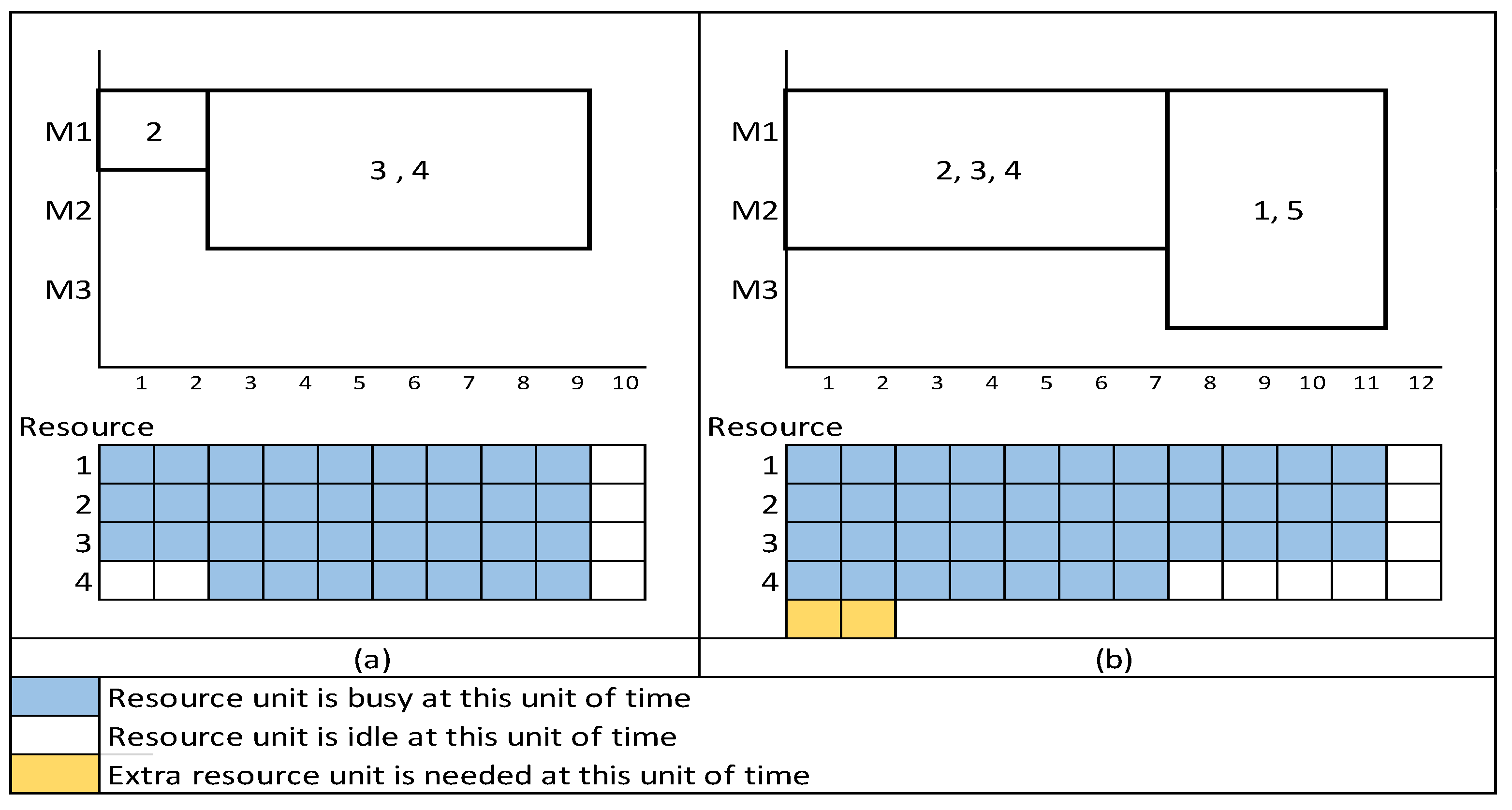
2.1. Problem Definition

This study considers a set of n jobs to be processed on m unrelated machines to minimize the maximum completion time. Each job has a certain processing unit time $p_{ik}$, where i and k are the indices for the job number and machine, respectively. Any machine can only process one job at a time. All jobs are not available at time zero and have their release dates $r_i.$Job preemption is not allowed, and there are no precedence relations among jobs. Every job has a setup time $s_{ijk}$ which depends on both the job sequence and the processing machine, that is, for any feasible schedule, if the job $i$is performed exactly after job $j$ on machine $k$. The amount of setup time will equal to $s_{ijk}$, and any change in job sequence or processing machine would change the setup value. The machines are not the only restricted resource. There are v renewable resources $R=\left\{R_1,R_2,\cdots ,R_v\right\}$. To process a job, a certain unit of resource is required per unit of time$Re{s}_{iv}$. Each resource has a limited capacity at any point in time. A job’s processing procedure cannot be started until both the assigned machine and allocated resources are available.

2.2. Lower Bound

To assess the performance and robustness of the proposed algorithms, one lower bound is developed in this study by using two lower bounds from other studies. First, the problem is simplified to be similar to a machine’s problem by selecting the minimum processing time and setup time for each job as given in Equations (1) and (2), respectively.

$$P_{\mathrm{i}}=\underset{k\in m}{\min }\left(p_{ik}\right),\forall i\in n,$$

(1)

$$S_i=\underset{k\in m}{\min }\left(\underset{j\in \left\{0,n\right\}}{\min }{s}_{jik}\right),\forall i\in n.$$

(2)

In the second equation, there is a zero in the j index to represent the dummy job j₀. This job was used to introduce the setup of the first job in the sequence.

The considered lower bounds are presented as follows:

2.2.1. First Lower Bound (LB1)

This lower bound is presented in the work of Afzalirad and Rezaeian [36]. The property is dependent on the capacity of each resource. The LB₁ is given in Equation (3).

$$L{B}_1={\stackrel{`}{LB}}_1+\lfloor \underset{\mathrm{i}\in \mathrm{n}}{\min }{\mathrm{r}}_{\mathrm{i}}+{\mathrm{S}}_{\mathrm{i}}/\mathrm{m}\rfloor ,$$

(3)

where:

$${\stackrel{`}{LB}}_1=\underset{\mathrm{v}\in \mathrm{R}}{\max }\left({\displaystyle \sum }_{{\mathrm{Res}}_{\mathrm{iv}}>\frac{{\mathrm{AR}}_{\mathrm{v}}}{2}}{\mathrm{P}}_{\mathrm{i}}+\frac{1}{2}{\displaystyle \sum }_{{\mathrm{Res}}_{\mathrm{iv}}=\frac{{\mathrm{AR}}_{\mathrm{v}}}{2}}{\mathrm{P}}_{\mathrm{i}}\right),$$

(4)

The ${\stackrel{`}{LB}}_1$ is obtained by computing the maximum expected time for each type of additional resource by considering only the jobs that occupy half of the resource capacity or more.

2.2.2. Second Lower Bound (LB2)

The second lower bound LB2 is defined by Equation (5), which was developed by the authors in this study. The LB2 was developed based on LB1, in which basic modification was introduced to LB2. As mentioned in LB1, for each type of additional resource, only jobs where the resource occupies half of the resource capacity or more are considered. However, LB2 considers all jobs.

$$L{B}_2={\stackrel{`}{LB}}_2+\lfloor \underset{i\in n}{\min }{r}_i+S_i/m\rfloor ,$$

(5)

where:

$${\stackrel{`}{LB}}_2=\underset{\mathrm{v}\in \mathrm{R}}{\max }\left(\frac{1}{2}{\displaystyle \sum }_{{\mathrm{Res}}_{\mathrm{iv}}\ge \frac{{\mathrm{AR}}_{\mathrm{v}}}{2}}{\mathrm{P}}_{\mathrm{i}}+\frac{1}{\mathrm{m}}{\displaystyle \sum }_{{\mathrm{Res}}_{\mathrm{iv}}<\frac{{\mathrm{AR}}_{\mathrm{v}}}{2}}{\mathrm{P}}_{\mathrm{i}}\right),$$

(6)

Proof. The jobs that occupy half of the resource capacity or more will determine half of the total processing time because these two types of jobs cannot be processed together at any time. Thus, for the jobs that occupy less than half of the resource capacity, the summation is calculated and divided by the number of machines.

2.2.3. Third Lower Bound (LB₃)

This lower bound is presented in the study by Qamhan et al. [37]. The property is dependent on the latest release date and given in Equation (7).

For any feasible schedule s,

$$LB{ }_3=\underset{\mathrm{i}}{\max }({\mathrm{r}}_{\mathrm{i}}+{\mathrm{P}}_{\mathrm{i}}+{\mathrm{S}}_{\mathrm{i}})\le {\mathrm{C}}_{\max },$$

(7)

Note: The lower bound of the problem is estimated by the maximum value among these three properties.

For further clarification, a numerical example is given to explain the lower bound e.g., five jobs (n = 5), three machines (m = 3), and one resource (R = 1), which are part of a scenario example that was implemented to further explain the existing lower bounds.

Table 1. Example input parameters.

Job	1	2	3	4	5
$r_i$	3	15	1	13	3
$p_{i1}$	8	6	5	7	7
$p_{i2}$	5	2	10	7	8
$p_{i3}$	4	4	7	8	7
$Re{s}_{i1}$	1	3	2	2	1	$R_1=4$

and

Table 2. Job/machines dependent setup time matrix.

Setup Times Matrix on Machine 1						Setup Times Matrix on Machine 2						Setup Times Matrix on Machine 3
Job	1	2	3	4	5	Job	1	2	3	4	5	Job	1	2	3	4	5
0	4	3	1	4	5	0	5	1	2	5	2	0	5	3	4	3	4
1	-	1	5	2	3	1	-	5	1	3	5	1	-	2	4	2	4
2	4	-	4	3	3	2	3	-	5	5	2	2	4	-	2	3	3
3	4	5	-	4	2	3	5	3	-	2	4	3	3	1	-	2	2
4	3	3	2	-	3	4	3	1	5	-	3	4	3	3	5	-	3
5	3	4	1	2	-	5	5	2	1	3	-	5	5	3	5	2	-

list the input parameters that are linked to the example.

After applying Equations (1) and (2), Table 1 and Table 2 were relaxed, as shown in

Table 3. The relaxed input parameters.

Job	1	2	3	4	5
$r_i$	3	15	1	13	3
$P_i$	5	2	5	7	7
$S_i$	3	1	1	2	2
$Re{s}_{i1}$	1	3	2	2	1	$R_1=4$

.

The first lower bound categorizes the job set under three subsets. In the first subset, where the number of resources exceeds half of the number of resources available, it can be seen that we have only one job (Job 2) for our example that satisfies this condition. In the second subset, where the number of resources is precisely equal to half of the number of resources available, Jobs 3 and 4 are under this subset. Finally, the rest of the jobs that are not selected from the two subsets will be ignored.

Figure 1a displays a Gantt map of the two subsets. While these two subsets cannot be processed at the same time due to the limitation of the number of resources available, the sum of all the jobs in the first subset will be taken as it is (summation of the first subset = 2). Subsequently, the second subset occupies precisely half the number of resources, so we take the sum of all the jobs in this subset and divide them by two to completely fill this resource (summation of the second subset = 12 divided by 2 equals 6). It is worth noting that if we have more than one resource, these actions will apply to all resources, and so the maximum total of the two subsets will be chosen as shown in Equation (4). From Equation (3), the first lower bound equals $\left(2+6\right)+\lfloor 1+9/2\rfloor =$ 13.

The second lower bound categorizes the set of jobs under two subsets. In the first subset, where the number of resources exceeds or equals half of the number of resources available, Jobs 2–4 are inside the subset. The second subset contains the rest of the jobs, which are 1 and 5. Figure 1b illustrates the Gantt chart of the two subsets. Machine 3 was idle when the first subset was under process because of the limitation of the number of resources. Because the jobs in this subset are equal to or exceed half of the number of resources, it will take half of the summation of the processing time to guarantee that at least this resource is fully occupied (2 + 5 + 7 = 14, then 14/2 = 7). For the second subset, if the limitation of the number of machines available is considered, then the summation of the processing time of this subset will be divided by the total number of machines (5 + 7 = 12, then 12/3 = 4). Similar to the first lower bound, if we have more than one resource, these procedures will be applied for all the resources, choosing the maximum total of two subsets outcome, as it is referred to in Equation (6). From Equation (5), the second lower bound equals $\left(7+4\right)+\lfloor 1+9/2\rfloor =$ 16.

The third lower bound takes the maximum summation of each job. From Equation (7), Job 4 has a maximum value equal to 22 because its release date equals 13, and the minimum processing time of the two machines with 7 units of time and a minimum dependent setup time equals 2.

3. Modified Harmony Search

The harmony search algorithm (HS) was introduced by Geem et al. [38]. HS is considered to be one of the metaheuristic algorithms that fall within population-based evolutions. This algorithm is inspired by the process of producing new musical melodies, which tries to find perfect harmony notes in a musical orchestra where each musician plays a note to identify better harmony. Musical performances are repeated to improvise harmony. The participating musicians act on their instruments to launch tones in their possible margin, thus creating a set of harmony vectors. In addition, in scheduling optimization, iterations continue to improve the solution and are evaluated according to their objective function. In each iteration, the jobs are assigned to the machine in different positions to generate a solution configuration.

Table 4. Comparison between musical and optimization processes.

Musical Process	Optimization Process
Musical harmony	Feasible solution
Musical improvisation	Iteration
Musical instrument	Decision variable
Tone	Value of a decision variable
Quality of harmony	Objective function

shows matching terminology for the processes executed in musical and optimization processes.

The HS algorithm has been successfully applied to several problems, and several extensions of the basic algorithm have been also proposed. In addition, Zammori et al. [35] introduced MHS, which has been successfully applied to manufacturing scheduling problems on single- and multiple-objective functions. In the following subsections, MHS is described in detail.

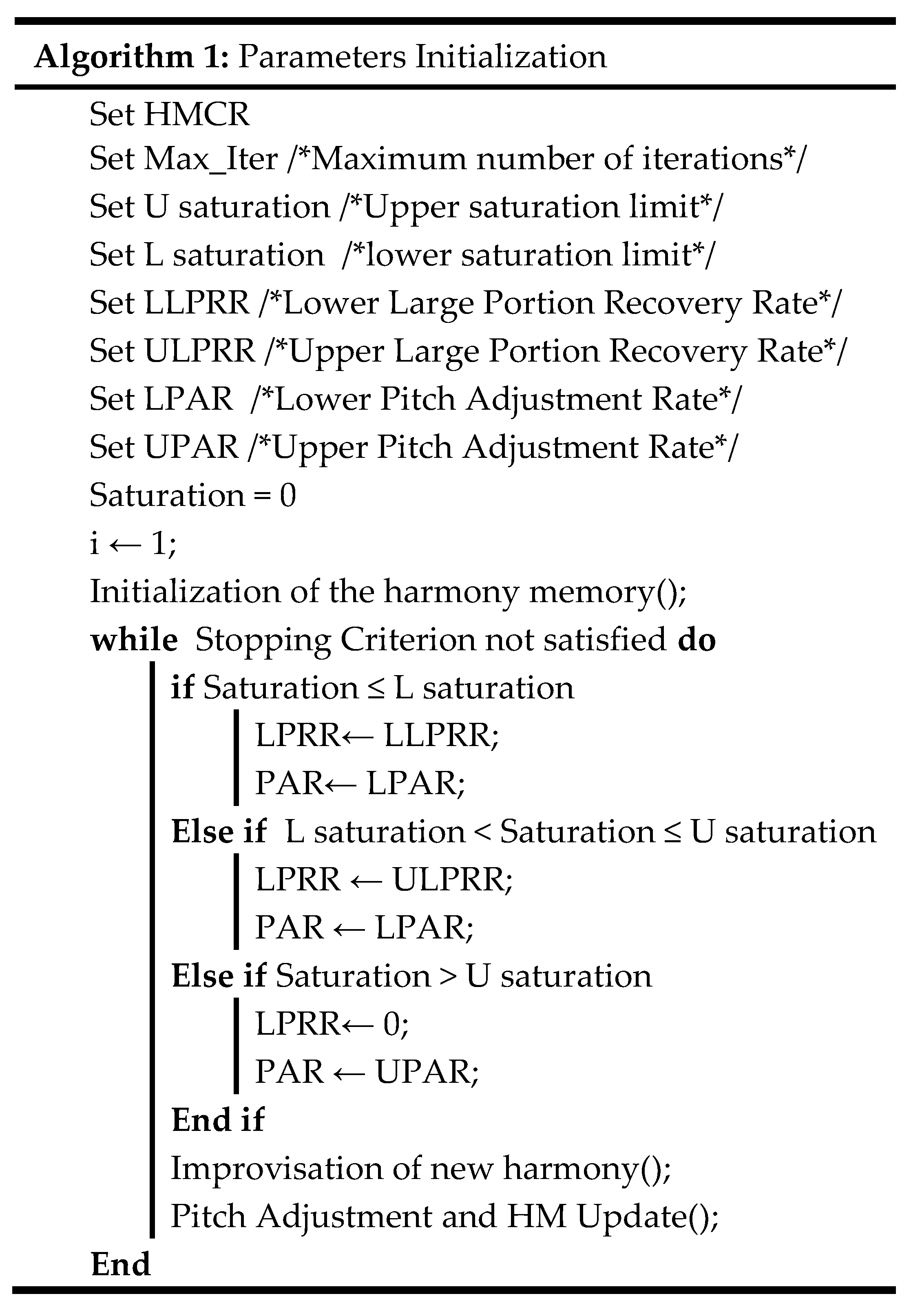
3.1. Initiation of the Parameters

The algorithm parameters are explained as follows:

• The harmony memory size (HMS) represents the number of solutions “rows” in the harmony matrix, which represents the actual repertoire of the musician.
• The harmony memory consideration rate (HMCR) represents the selection rate for the new element from the ith column of the harmony matrix HM by considering the goodness of objective function. This parameter imitates the artist’s behavior, where most of them tend to reuse parts of the past work “repertoire.”
• The purpose of pitch adjustment rate (PAR) is to select a random job and change its positions in its neighborhood. Pitch adjustment mimics the slight modification by the artist of melodies for some notes. PAR is used after a new solution is built and can be applied to each job position of the solution. In this case, the position of each job can be modified with PAR probability.
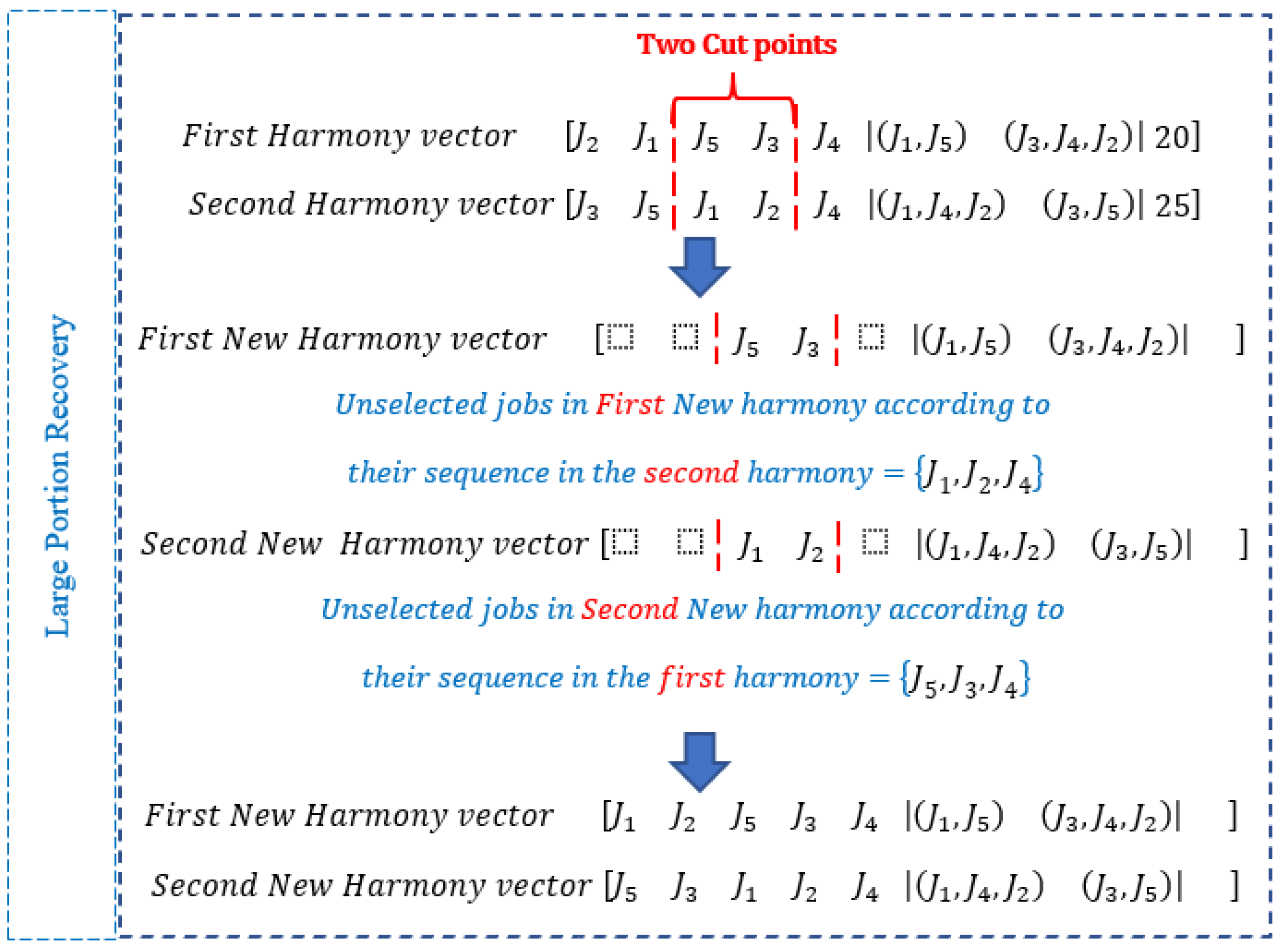
• Large portion recovery (LPR) was introduced by Zammori et al. [35] as a new feature in MHS. This feature tries to mimic the human nature of a musician, who mixes different earlier melodies or reuses their large sequence to create new harmonies.
• Saturation is also a new feature that is presented in MHS by Zammori et al. [35]. The purpose of computing saturation is to help the search process escape being trapped in local optima in which the similarity of HM vectors is tested. When the value of saturation is equal to zero, all the vectors in HM are different. In addition, saturation is computed as follows:

$$Saturation= \frac{Number of vectors with a copy within the HM}{HMS- 1}$$

(8)

• Stopping criterion for the search is when a specific number of iterations is reached without improvement (No_imp).

The steps for the MHS algorithm are described in Figure 2.

We had nine parameters for our algorithm to control its performance. Three parameters were fixed as long as the algorithm is running, which are the HMS, HMCR, and the stopping criteria. For pitch adjustment rate (PAR) and the large portion recovery rate (LPRR) will be redefined in high and low levels. High pitch adjustment (HPAR), low pitch adjustment (LPAR), high large portion recovery (HLPRR), and low large portion recovery (LLPRR) will be picked for each rate according to the saturation percentage for each iteration. As stated earlier, saturation is a relationship based on the number of vectors with a copy within the HM, so we will have two parameters to handle saturation variability: high saturation (HSat), and low saturation (LSat). In any iteration, if the saturation percentage is less than the LSat, then the LPRR is equal to the LLPRR, and the PAR is equal to the LPAR. Otherwise, if the saturation percentage is greater than LSat and smaller than HSat, the LPRR is equivalent to ULPRR, and the PAR is equal to LPAR. Finally, if the saturation percentage is greater than HSat, the LPRR is equal to zero, and the PAR is equal to HPAR. It is noteworthy that the change in saturation is intended to help the search phase escape from being stuck in the local optima in which the similarity of HM vectors is checked.

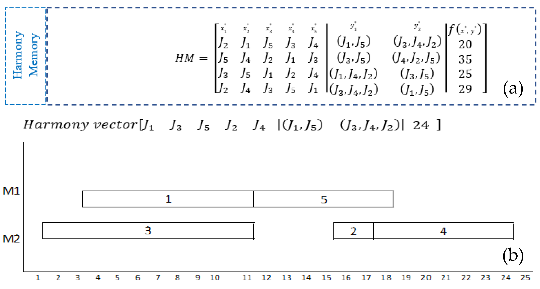
3.2. Initialization of Harmony Memory

In this step, a set of HMS solutions is randomly generated. For each solution, the objective function is calculated. The equation shows the general structure of HM. This memory can be considered a matrix containing a set of harmonies or solutions. During this step, harmony memory is generated. Each job is randomly assigned to the position from its choice list. For each solution, it corresponds to a value of the fitness function as shown in the following equation:

$$HM=\left[\begin{array}{ccccccc}{x}_1^1& & x_2^1& & \cdots & & x_n^1\\ x_1^2& & x_2^2& & \cdots & & x_n^2\\ \cdots & & \cdots & & \cdots & & \cdots \\ \cdots & & \cdots & & \cdots & & \cdots \\ x_1^{\mathit{HMS}}& & x_2^{\mathit{HMS}}& & \cdots & & x_n^{\mathit{HMS}}\end{array}\begin{array}{c}\text{|}\\ \text{|}\\ \text{|}\\ \text{|}\\ \text{|}\end{array}\begin{array}{ccccccc}{y}_1^1& & y_2^1& & \cdots & & y_m^1\\ y_1^2& & y_2^2& & \cdots & & y_m^2\\ \cdots & & \cdots & & \cdots & & \cdots \\ \cdots & & \cdots & & \cdots & & \cdots \\ y_1^{\mathit{HMS}}& & y_2^{\mathit{HMS}}& & \cdots & & y_m^{\mathit{HMS}}\end{array}\begin{array}{c}\text{|}\\ \text{|}\\ \text{|}\\ \text{|}\\ \text{|}\end{array}\begin{array}{c}f(x^1)\\ f(x^2)\\ \text{⋯}\\ \text{⋯}\\ f\left(x^{HMS}\right)\end{array}\right]$$

(9)

where $x_i^h$ is the ith job position in the h row, $y_k^h$ is a vector that represents the jobs that processed on machine k in the h rows, and $f\left(x^h\right)$ represents the objective function of h row.

Figure 3 shows an example of changing harmony search to harmony memory and Gantt chart.

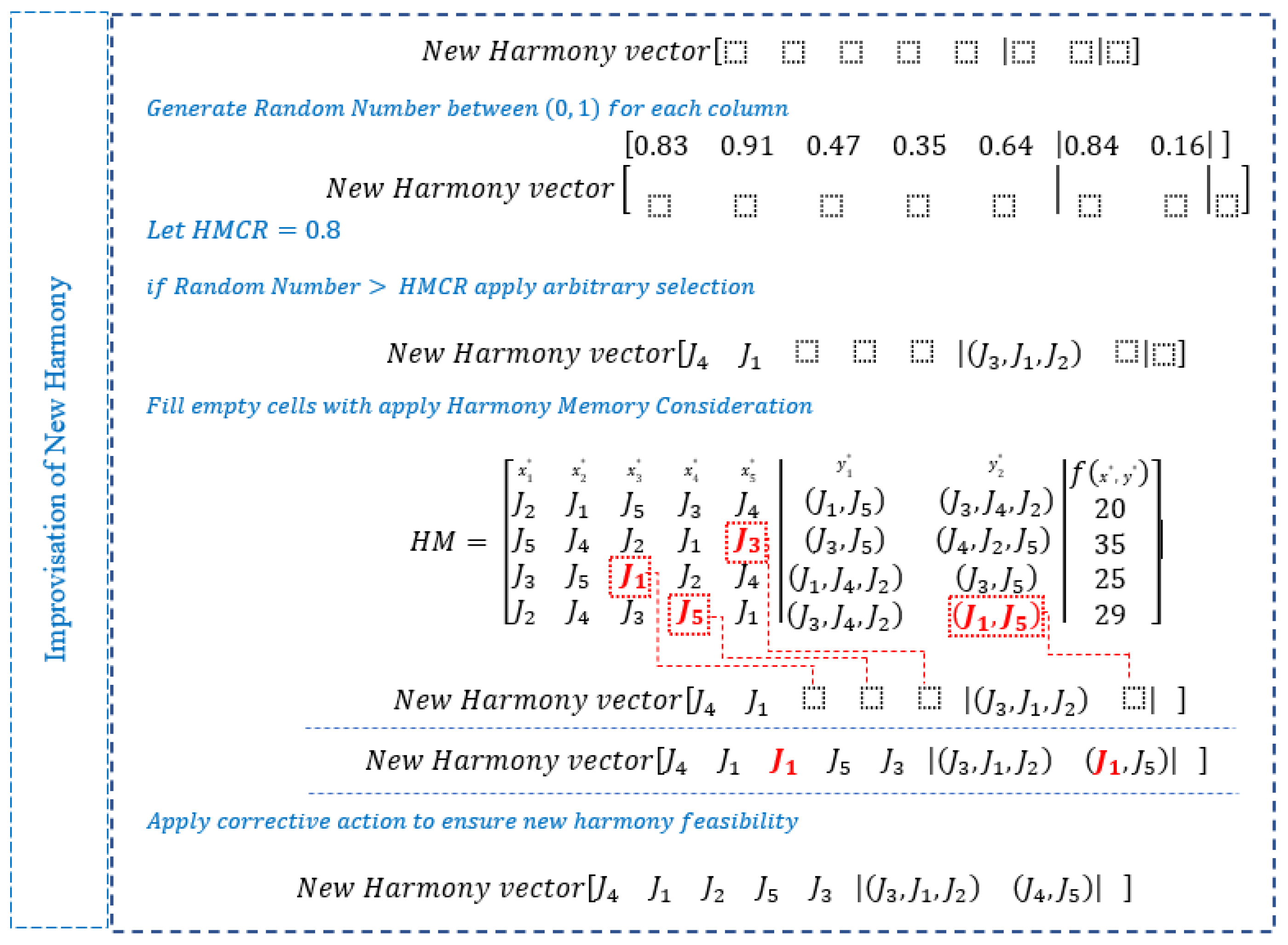
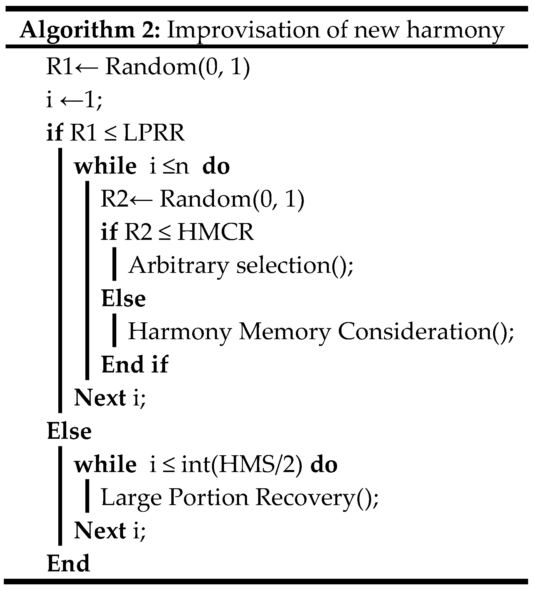
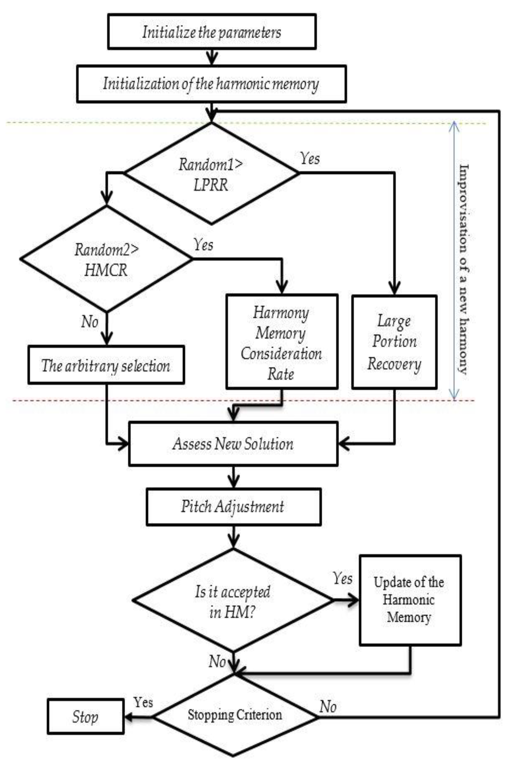
3.3. Improvisation of New Harmony

A new solution is generated by matrix HM using the parameters HMCR, PAR, and LRP that were defined in Section 3.1. These settings will help the algorithm to obtain local or global enhanced solutions. The solution is constructed using the following three rules:

3.3.1. Arbitrary Selection

The arbitrary selection process generates a new harmony vector $x_i^{*}$ and $y_j^{*}$ by selecting them randomly.

3.3.2. Harmony Memory Consideration Rate (HMCR)

The value for HMCR varies between 0 and 1. As mentioned earlier, this imitates the artist’s behavior of tending to reuse parts of the past work “repertoire.” Each component in the new harmony vector $x_i^{*}$ and $y_j^{*}$ is determined from the job and sequence on the machine of ith and jth columns of HM, respectively (with HMCR probability).

The above is illustrated in Figure 4 below:

3.3.3. Large Portion Recovery (LPR)

As mentioned earlier, instead of replicating a single note at a time, LPR was introduced to generate new harmonies by reusing entire subarrays of notes, which means that two-point crossover for the best harmonies available within HM.

The steps for the improvisation of the New Harmony algorithm are given in Figure 5, and Figure 6 is an example of the large portion recovery.

3.4. Pitch Adjustment Rate

The procedure of this method is to select a random job and change its position in its neighborhood. In this case, the position of each job can be modified by PAR probability.

3.5. Update Harmony Memory and Stopping Criterion

The new solution must be checked for the violation of constraints of the problem. The new solution is added to harmony memory if it is better than the worst harmony solution in HM in terms of fitness. Then, the worst solution is removed from HM. If the stopping criterion is reached, then the search will stop, and the algorithm is completed. Figure 7 shows the flowchart for the modified harmony search algorithm.

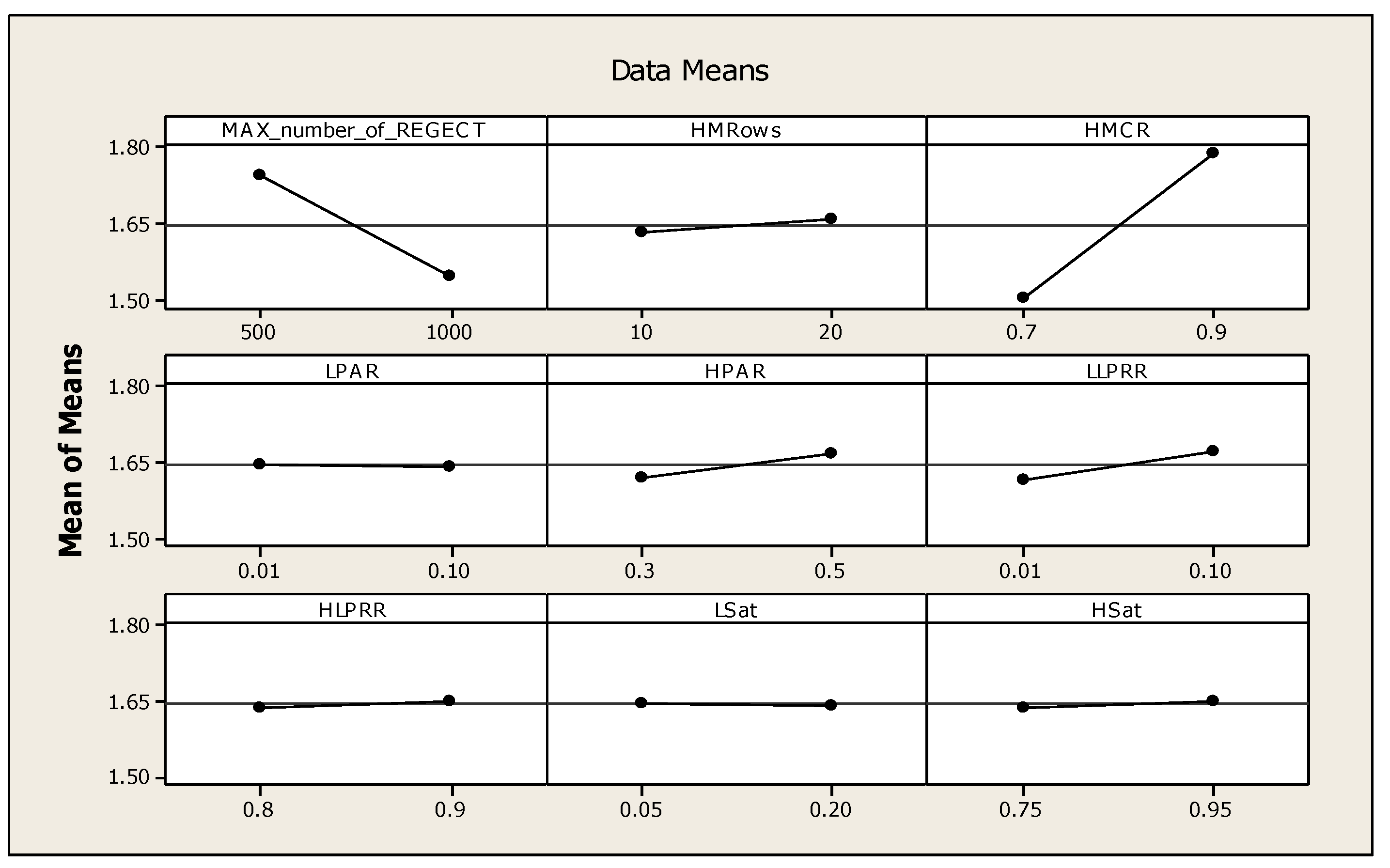
3.6. Tuning of Parameters for MHS

A Taguchi design of L12 analysis is applied to study the effect of MHS parameters. One instance for each combination n*m*R was generated randomly to conduct the best tune of the MHS parameters. It is worth noting that the different levels for the generated data were used in the computational data set generation in the following section. The number of jobs are n = {30, 40, and 50}, the number of machines are m = {4, 6, and 8}, and the number of additional resources are R = {1, 2, and 3}. In addition, the average relative percentage deviation (ARPD) was used as the response variable of factorial analysis. The test parameters used in this experiment are listed in

Table 5. MHS factors and their two levels.

Parameters	Level
	Low	High
MAX_number_of_REGECT	500	1000
HMRows	10	20
HMCR	0.7	0.9
LPAR	0.01	0.1
HPAR	0.3	0.5
LLPRR	0.01	0.1
HLPRR	0.8	0.9
LSat	0.05	0.2
HSat	0.75	0.95

below.

From Figure 8, it is clear that there are two critical factors, which are Max_number_of_REGECT, and HMCR. This means that there is a significant effect of these factors on the MHS performance.

Based on the results in Figure 8, the recommended values of the different parameters will be as follows: Max_number_of_REGECT = 1000, HMCR = 0.7, and HMRows = 10.

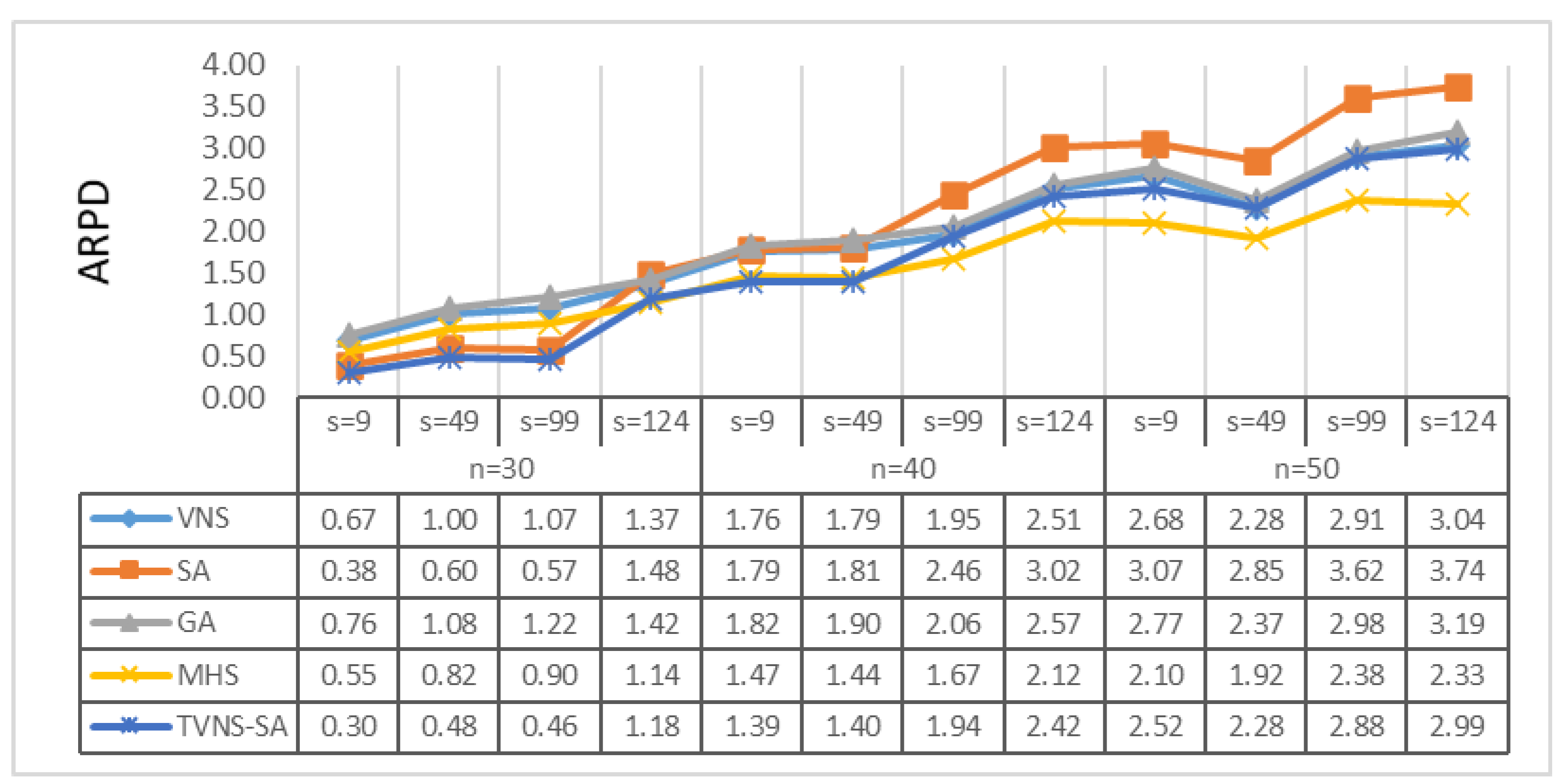
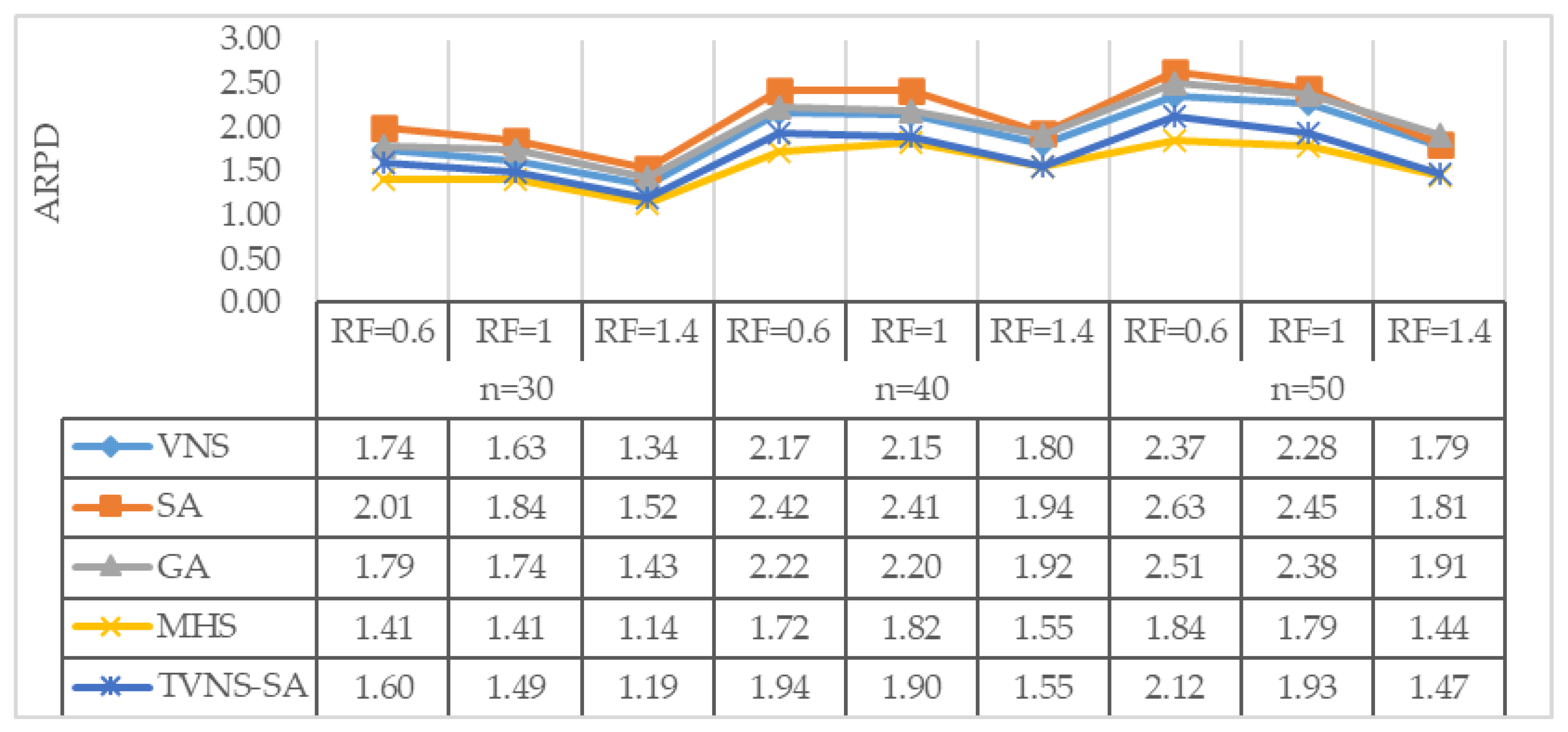
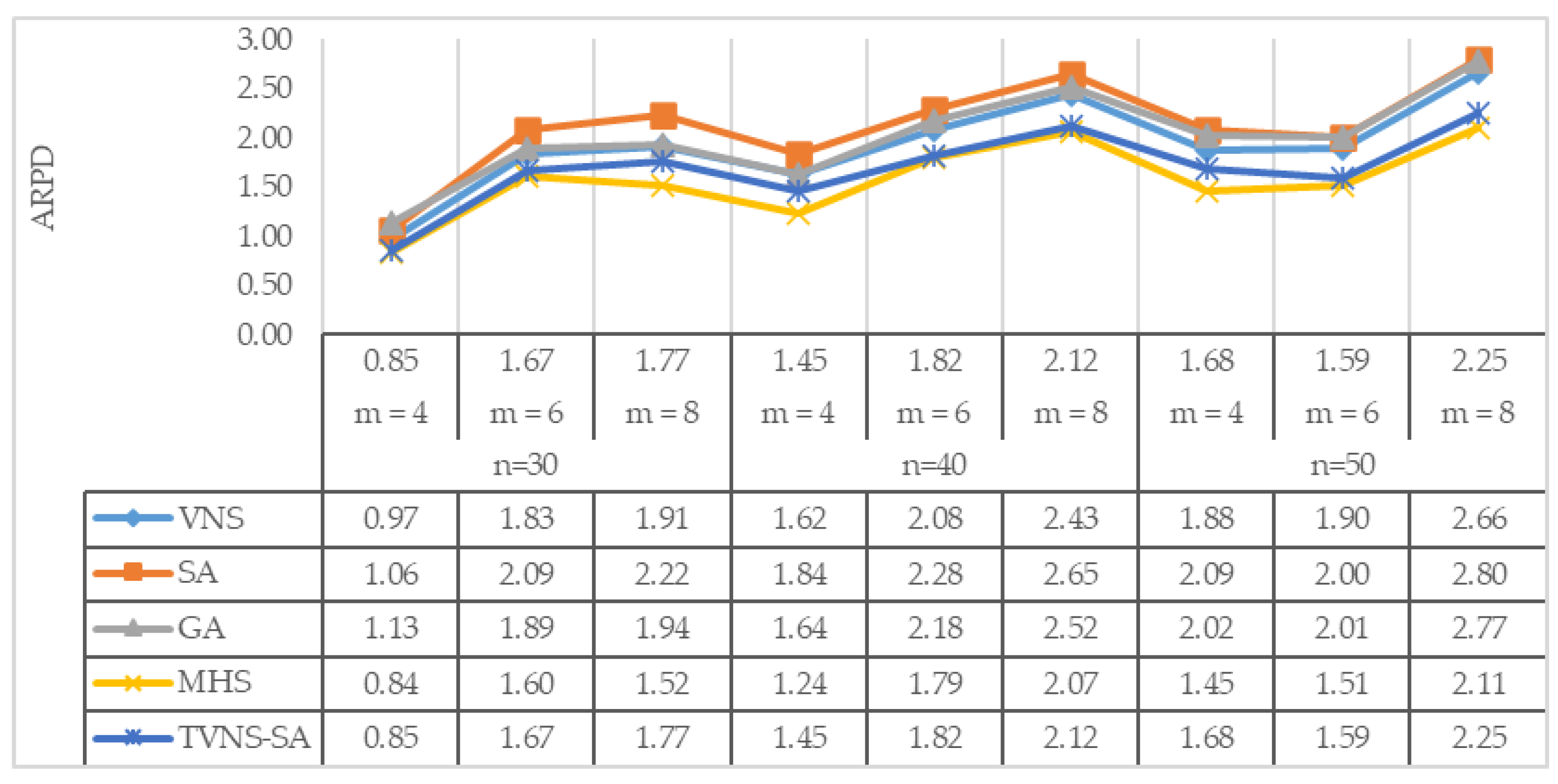
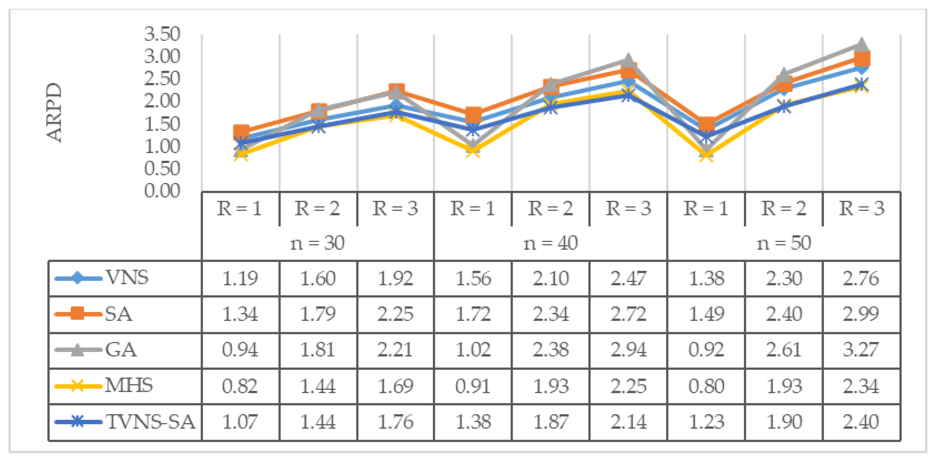
4. Computational Results

In this study, the MHS algorithm was coded in C and ran on a PC with Intel^® Core™ i7-7700HQ CPU @280 GHz and 8 GB of RAM (MSI MS16JD, Taipei, Taiwan).

The performance of MHS was evaluated by conducting extensive experimentations using different problem instances. A total of 324 instances was generated using different levels and conditions for each parameter. For each instance, different levels of number of jobs, number of machines (m), and number of additional resources (R) were generated. The different levels for the number of jobs are n = {30, 40, and 50}. Three different levels for the number of machines, which are m = {4, 6, and 8}. Finally, the different levels for the number of additional resources are R = {1, 2, and 3}.

Table 6. The generating conditions of Second test instances.

Group	Parameter Range	Reference Paper
Processing times	U(1, 99)	Vallada and Ruiz [39]
Setup times	U(1, 9), U(1, 49), U(1, 99), and U(1, 124)
Release dates	U (1, L) Where L is computed as L = n*ρ*Rf/m n = number of jobs and m = number of machines ρ = expected processing time Release range factor (Rf) = { 0.6, 1.0, 1.4}	Velez-Gallego et al. [40]
The available amount of each resource (AR)	U(1, 5)	Afzalirad and Rezaeian [36]
Resource requirements	U(0, AR)

shows the different levels for other parameters for each instance in which these pentameters are as follows: processing times, setup times, release dates, available amount of each resource, and resource requirements. As shown in the last column of Table 6, the ranges for these parameters were adopted from Vallada and Ruiz [39], Vélez-Gallego et al. [40], and Afzalirad and Rezaeian [36].

The main computational result indicators that are taken into consideration are:

• Average relative percentage deviation (ARPD): average gap “RPD” between the obtained result;
• Lower bound for all instances with the same level of generation condition.

$$\mathrm{RPD}=\frac{\left|{\mathrm{Algorithm}}_{\mathrm{sol}}-\mathrm{lower}\mathrm{bound}\right|}{\mathrm{lower}\mathrm{bound}}$$

(10)

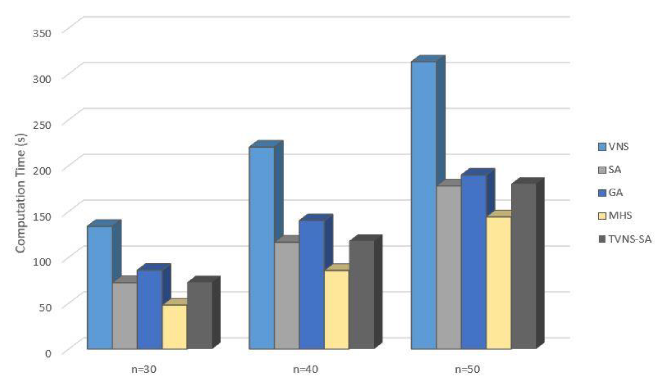
• CPU running time: consumed time for an algorithm to obtain the final result

The performance of MHS was compared with several algorithms, which have been proposed in the literature to solve similar problems to the one investigated in this paper. These algorithms are as follows: the standard simulated annealing (SA), the variable neighborhood search (VNS), the hybrid two-stage variable neighborhood with simulated annealing proposed by Al-harkan and Qamhan [41], and the fourth method is the genetic algorithm (GA) similar to the work of Afzalirad and Rezaeian [36]. Finally, with the help of the MINITAB V16 software (V16, Minitab, United Kingdom), Taguchi analysis is applied to the different algorithms to guarantee that these algorithms are also fine-tuned in their parameters fairly well. A summary of the main parameters and their levels is shown in

Table 7. The main parameters of other different algorithms.

Algorithm	Parameter	Considered Values	Selected Values
SA	Initial temperature	100–1000	100
	Cooling rate	0.009–0.09	0.09
	Stopping condition	Number of nonimprovements (150–300)	300
VNS	Number of neighborhoods	10–20	10
	Number of nonimprovements in the local search	150–300	300
HTVN-SA	Initial temperature	100–1000	100
	Cooling rate	0.009–0.09	0.09
	Number of neighborhoods	10–20	10
	Number of nonimprovements in the local search	150–300	300
GA	Population size	40, 50, 60	50
	Crossover rate (Pc)	0.6, 0.75, 0.9	0.75
	Mutation rate (Pm)	0.05, 0.15, 0.25	0.25
	Stopping condition	Maximum iterations (120, 170, 220)	220

.

The computational results are summarized in Figure 9, Figure 10, Figure 11 and Figure 12, in which the performance of the MHS algorithm was compared with those of the other four metaheuristics. In Figure 9, the comparison was conducted using the different levels of setup times. The results show that ARPD increases with the increase of the setup time and the number of jobs, which indicates that both the setup time and number of jobs are significant parameters. In addition, the deviation among all algorithms in the ARPD increases as long as the setup time and number of jobs increase. Figure 9 also indicates that the two-stage hybrid variable neighborhood search with simulated annealing (TVNS-SA) and SA outperform the MHS regarding ARPD for the instances that have a setup time range between (1 and 9), (1 and 49), or (1 and 99) and the number of jobs equals 30 or 40. However, when the setup time range is bigger than these ranges, the MHS outperforms the TVNS-SA. In Figure 10, the range of release times is used for comparison. The figures show that ARPD decreases with the increase of RF while n was not a significant parameter for the ARPD. The number of machines and the number of resources were used for comparison in Figure 11 and Figure 12. In these two figures, ARPD increases with the increase of m and r. There was also a slight increase in n as well; however, it is not a significant parameter. These figures show that the MHS algorithm outperforms all metaheuristic algorithms with respect to objective function values.

With the help of the MINITAB V16 software (V16, Minitab, United Kingdom), a paired t-test was used to test the difference between the performances of MHS and TVNS-SA due to their close performance, as indicated in Figure 9, Figure 10, Figure 11 and Figure 12. Figure 13 and Figure 14 show that with a 95% confidence interval, the difference between the performances of MHS and TVNS-SA could not be zero. This fact shows that the performances of MHS and TVNS-SA are significantly different.

Figure 15 shows the CPU time required by each algorithm. It is clear that the proposed MHS was able to obtain the exact solutions in reasonable CPU times. In addition, it was able to outperform the other three metaheuristics with respect to CPU time. One of the reasons why is HS used all the vectors in the Harmony Memory in each iteration, while GA used only two parents in each iteration. Due to this, it was shown that the CPU is less. In addition, an HS feature is that it reaches a better solution with a lesser number of functions.

It is worth mentioning that most of the previous studies from the literature used ARPD and CPU time as the only performance indicators, while this study added the overall percentage of different algorithms as a new indicator (Figure 16). There is a difference between ARPD and the overall percentage of different algorithms. ARPD provides the best average percentage deviation from the lower bound, while the overall percentage of different algorithms provides the comparison between the different algorithms concerning its number of instances for which the algorithm gave better solutions than the other divided by the total number of instances. In our study, we have about 324 instances, and according to the ARPD, it can be concluded that the MHS outperforms all the other algorithms (see Figure 9, Figure 10, Figure 11 and Figure 12). However, if we count the number of instances for which the algorithm gave better solutions than the other, the MHS had about 136 instances from 324 (42%), so it is recommended to add an overall percentage of different algorithms as a performance indicator besides ARPD in future studies.

HS has a good exploration of in-depth searching in the local optimal solution and exploitation, which search criteria in a wider range even if it moves from the local optima solution. From the result of the overall percentage of different algorithms, it achieved 42% but at the same time having a small deviation. It is worth noting that MHS gathered both HS and GA in large portion recovery, and this is to ensure the criteria of good exploration and exploitation. In addition, one of the limitations is that as long as the number of jobs and setup time increase, the deviation in the ARPD also increases.

5. Conclusions

In this study, an adopted harmony search approach was developed to minimize the makespan for unrelated parallel machines with multiple renewable resources, sequence-dependent setup times, and release date constraints. The performance of the MHS algorithm was compared with those of several other algorithms such as variable neighborhood search (VNS), two-stage hybrid variable neighborhood search with simulated annealing (TVNS-SA), simulated annealing (SA), and genetic algorithm (GA). The proposed MHS algorithm was able to outperform the other four metaheuristics whether the parameter was significant or not with respect to the average relative percentage deviation (ARPD). It performed best within a large number of jobs, so it is therefore recommended in cases of problems that have a large job number. In addition, MHS outperformed the other four algorithms with respect to CPU time, which is essential and practical in problem solving. Benchmarking data in previous studies were for lower ranges, while in the current study, the benchmarking data were for a much higher range, which closely simulates practical problems. Future work can use the data in the current study to compare with the previous ones. The deviation of the ARPD increased with the increase of the job number and the setup time. This can be one of the potential ideas for future work by the use of an optimization method while adopting some useful algorithms knowledge.

References

1. Liu, P.; Gong, H.; Fan, B.; Rudek, R.; Damodaran, P.; Tang, G. Recent advances in scheduling and its applications. Discret. Dyn. Nat. Soc. 2015, 2015, 1–2. [Google Scholar] [CrossRef]
2. Afzalirad, M.; Rezaeian, J.J.E.O. Design of high-performing hybrid meta-heuristics for unrelated parallel machine scheduling with machine eligibility and precedence constraints. Eng. Optim. 2016, 48, 706–726. [Google Scholar] [CrossRef]
3. Bitar, A.; Dauzère-Pérès, S.; Yugma, C.; Roussel, R.J.J.O.S. A memetic algorithm to solve an unrelated parallel machine scheduling problem with auxiliary resources in semiconductor manufacturing. J. Sched. 2016, 19, 367–376. [Google Scholar] [CrossRef] [Green Version]
4. Allahverdi, A.; Gupta, J.N.D.; Aldowaisan, T. A review of scheduling research involving setup considerations. Omega-Int. J. Manag. S 1999, 27, 219–239. [Google Scholar] [CrossRef]
5. Allahverdi, A.; Ng, C.; Cheng, T.E.; Kovalyov, M.Y. A survey of scheduling problems with setup times or costs. Eur. J. Ope.r Res. 2008, 187, 985–1032. [Google Scholar] [CrossRef] [Green Version]
6. Allahverdi, A. The third comprehensive survey on scheduling problems with setup times/costs. Eur. J. Oper. Res. 2015, 246, 345–378. [Google Scholar] [CrossRef]
7. Lin, S.W.; Ying, K.C. ABC-based manufacturing scheduling for unrelated parallel machines with machine-dependent and job sequence-dependent setup times. Comput. Oper. Res. 2014, 51, 172–181. [Google Scholar] [CrossRef]
8. Ezugwu, A.E.; Akutsah, F. An Improved Firefly Algorithm for the Unrelated Parallel Machines Scheduling Problem with Sequence-Dependent Setup Times. IEEE Access 2018, 6, 54459–54478. [Google Scholar] [CrossRef]
9. Afzalirad, M.; Rezaeian, J. A realistic variant of bi-objective unrelated parallel machine scheduling problem: NSGA-II and MOACO approaches. Appl. Soft Comput. 2017, 50, 109–123. [Google Scholar] [CrossRef]
10. Weng, M.X.; Lu, J.; Ren, H.Y. Unrelated parallel machine scheduling with setup consideration and a total weighted completion time objective. Int. J. Prod. Econ. 2001, 70, 215–226. [Google Scholar] [CrossRef]
11. Lin, Y.K.; Hsieh, F.Y. Unrelated parallel machine scheduling with setup times and ready times. Int. J. Prod. Res. 2014, 52, 1200–1214. [Google Scholar] [CrossRef]
12. Emami, S.; Moslehi, G.; Sabbagh, M. A Benders decomposition approach for order acceptance and scheduling problem: A robust optimization approach. Comput. Appl. Math. 2017, 36, 1471–1515. [Google Scholar] [CrossRef]
13. Bektur, G.; Sarac, T. A mathematical model and heuristic algorithms for an unrelated parallel machine scheduling problem with sequence-dependent setup times, machine eligibility restrictions and a common server. Comput. Oper. Res. 2019, 103, 46–63. [Google Scholar] [CrossRef]
14. Obeid, A.; Dauzere-Peres, S.; Yugma, C. Scheduling job families on non-identical parallel machines with time constraints. Ann. Oper. Res. 2014, 213, 221–234. [Google Scholar] [CrossRef]
15. Zeidi, J.R.; MohammadHosseini, S. Scheduling unrelated parallel machines with sequence-dependent setup times. Int. J. Adv. Manuf. Technol. 2015, 81, 1487–1496. [Google Scholar] [CrossRef]
16. Rabadi, G.; Moraga, R.J.; Al-Salem, A. Heuristics for the unrelated parallel machine scheduling problem with setup times. J. Intell. Manuf. 2006, 17, 85–97. [Google Scholar] [CrossRef]
17. Hamzadayi, A.; Yildiz, G. Modeling and solving static m identical parallel machines scheduling problem with a common server and sequence dependent setup times. Comput. Ind. Eng. 2017, 106, 287–298. [Google Scholar] [CrossRef]
18. Edis, E.B.; Oguz, C.; Ozkarahan, I. Parallel machine scheduling with additional resources: Notation, classification, models and solution methods. Eur. J. Oper. Res. 2013, 230, 449–463. [Google Scholar] [CrossRef]
19. Gyorgyi, P. A PTAS for a resource scheduling problem with arbitrary number of parallel machines. Oper. Res. Lett. 2017, 45, 604–609. [Google Scholar] [CrossRef] [Green Version]
20. Gyorgyi, P.; Kis, T. Approximability of scheduling problems with resource consuming jobs. Ann. Oper. Res. 2015, 235, 319–336. [Google Scholar] [CrossRef] [Green Version]
21. Gyorgyi, P.; Kis, T. Approximation schemes for parallel machine scheduling with non-renewable resources. Eur. J. Oper. Res. 2017, 258, 113–123. [Google Scholar] [CrossRef] [Green Version]
22. Hebrard, E.; Huguet, M.J.; Jozefowiez, N.; Maillard, A.; Pralet, C.; Verfaillie, G. Approximation of the parallel machine scheduling problem with additional unit resources. Discret. Appl. Math 2016, 215, 126–135. [Google Scholar] [CrossRef] [Green Version]
23. Kis, T. Approximability of total weighted completion time with resource consuming jobs. Oper. Res. Lett. 2015, 43, 595–598. [Google Scholar] [CrossRef] [Green Version]
24. Zheng, X.L.; Wang, L. A two-stage adaptive fruit fly optimization algorithm for unrelated parallel machine scheduling problem with additional resource constraints. Expert Syst. Appl. 2016, 65, 28–39. [Google Scholar] [CrossRef]
25. Afzalirad, M.; Shafipour, M. Design of an efficient genetic algorithm for resource-constrained unrelated parallel machine scheduling problem with machine eligibility restrictions. J. Intell. Manuf. 2018, 29, 423–437. [Google Scholar] [CrossRef]
26. Vallada, E.; Villa, F.; Fanjul-Peyro, L. Enriched metaheuristics for the resource constrained unrelated parallel machine scheduling problem. Comput. Oper. Res. 2019, 111, 415–424. [Google Scholar] [CrossRef]
27. Li, K.; Yang, S.L.; Leung, J.Y.T.; Cheng, B.Y. Effective meta-heuristics for scheduling on uniform machines with resource-dependent release dates. Int. J. Prod. Res. 2015, 53, 5857–5872. [Google Scholar] [CrossRef]
28. Abdeljaoued, M.A.; Saadani, N.E.H.; Bahroun, Z. Heuristic and metaheuristic approaches for parallel machine scheduling under resource constraints. Oper. Res. 2018, 20, 1–24. [Google Scholar] [CrossRef]
29. Ozpeynirci, S.; Gokgur, B.; Hnich, B. Parallel machine scheduling with tool loading. Appl. Math. Model. 2016, 40, 5660–5671. [Google Scholar] [CrossRef]
30. Furugyan, M.G. Optimal correction of execution intervals for multiprocessor scheduling with additional resource. J. Comput. Syst. Sci. Int. 2015, 54, 268–277. [Google Scholar] [CrossRef]
31. Dosa, G.; Kellerer, H.; Tuza, Z. Restricted assignment scheduling with resource constraints. Theor. Comput. Sci. 2019, 760, 72–87. [Google Scholar] [CrossRef] [Green Version]
32. Wang, Y.C.; Wang, M.J.; Lin, S.C. Selection of cutting conditions for power constrained parallel machine scheduling. Robot. Comput.-Integr. Manuf. 2017, 43, 105–110. [Google Scholar] [CrossRef]
33. Labbia, W.; Boudhara, M.; Oulamara, A. Scheduling two identical parallel machines with preparation constraints. Int. J. Prod. Res. 2017, 55, 1531–1548. [Google Scholar] [CrossRef]
34. Li, J.Q.; Duan, P.Y.; Sang, H.Y.; Wang, S.; Liu, Z.M.; Duan, P. An Efficient Optimization Algorithm for Resource-Constrained Steelmaking Scheduling Problems. IEEE Access 2018, 6, 33883–33894. [Google Scholar] [CrossRef]
35. Zammori, F.; Braglia, M.; Castellano, D. Harmony search algorithm for single-machine scheduling problem with planned maintenance. Comput. Ind. Eng. 2014, 76, 333–346. [Google Scholar] [CrossRef]
36. Afzalirad, M.; Rezaeian, J. Resource-constrained unrelated parallel machine scheduling problem with sequence dependent setup times, precedence constraints and machine eligibility restrictions. Comput. Ind. Eng. 2016, 98, 40–52. [Google Scholar] [CrossRef]
37. Qamhan, M.A.; Qamhan, A.A.; Al-Harkan, I.M.; Alotaibi, Y.A. Mathematical Modeling and Discrete Firefly Algorithm to Optimize Scheduling Problem with Release Date, Sequence-Dependent Setup Time, and Periodic Maintenance. Math. Probl. Eng. 2019, 2019. [Google Scholar] [CrossRef] [Green Version]
38. Geem, Z.W.; Kim, J.H.; Loganathan, G.V. A new heuristic optimization algorithm: Harmony search. Simulation 2001, 76, 60–68. [Google Scholar] [CrossRef]
39. Vallada, E.; Ruiz, R. A genetic algorithm for the unrelated parallel machine scheduling problem with sequence dependent setup times. Eur. J. Oper. Res. 2011, 211, 612–622. [Google Scholar] [CrossRef] [Green Version]
40. Velez-Gallego, M.C.; Maya, J.; Torres, J.R.M. A beam search heuristic for scheduling a single machine with release dates and sequence dependent setup times to minimize the makespan. Comput. Oper. Res. 2016, 73, 132–140. [Google Scholar] [CrossRef]
41. Al-Harkan, I.M.; Qamhan, A.A. Optimize Unrelated Parallel Machines Scheduling Problems With Multiple Limited Additional Resources, Sequence-Dependent Setup Times and Release Date Constraints. IEEE Access 2019, 7, 171533–171547. [Google Scholar] [CrossRef]
Figure 1. Illustration for the lower bound where M1-M3 are machines: (a) first lower bound; (b) second lower bound.
Processes 09 00654 g001
Figure 2. Parameters initialization algorithm.
Processes 09 00654 g002
Figure 3. Harmony search examples for (a) an example of Harmony Memory; (b) visualized vector in Gantt chart.
Processes 09 00654 g003
Figure 4. Example of improvisation of New Harmony.
Processes 09 00654 g004
Figure 5. Improvisation of the New Harmony algorithm.
Processes 09 00654 g005
Figure 6. Example of large portion recovery procedures.
Processes 09 00654 g006
Figure 7. Modified harmony search (MHS) flowchart.
Processes 09 00654 g007
Figure 8. MHS main effects plot for the different factors.
Processes 09 00654 g008
Figure 9. Computational results with a different range of setup times.
Processes 09 00654 g009
Figure 10. Computational results with a different range of release dates.
Processes 09 00654 g010
Figure 11. Computational results with a different number of resources.
Processes 09 00654 g011
Figure 12. Computational results with a different number of machines.
Processes 09 00654 g012
Figure 13. Paired t-test for the MHS and two-stage hybrid variable neighborhood search with simulated annealing (TVNS-SA) performance differences.
Processes 09 00654 g013
Figure 14. Histogram of differences for MHS and TVNS-SA performance.
Processes 09 00654 g014
Figure 15. Computational CPU running times for algorithms.
Processes 09 00654 g015
Figure 16. Overall percentage of different algorithms.
Processes 09 00654 g016