Article

A Finite Element Simulation of the Active and Passive Controls of the MHD Effect on an Axisymmetric Nanofluid Flow with Thermo-Diffusion over a Radially Stretched Sheet

1
Department of Applied Mathematics, School of Science, Northwestern Polytechnical University, Dongxiang Road, Chang’an District, Xi’an 710129, China
2
School of Automation, Northwestern Polytechnical University, 127 West Youyi Road, Xi’an 710072, China
3
College of Internet of Things Engineering, Hohai University, Changzhou Campus, Changzhou 213022, China
4
School of Energy and Power, Xi’an Jiaotong University, No.28 Xianning West Road, Xi’an 7100049, China
*
Author to whom correspondence should be addressed.
Bagh Ali and Xiaojun Yu are co-first authors.
Processes 2020, 8(2), 207; https://doi.org/10.3390/pr8020207
Submission received: 20 November 2019 / Revised: 14 January 2020 / Accepted: 3 February 2020 / Published: 7 February 2020

Abstract

:
The present study investigated the steady magnetohydrodynamics of the axisymmetric flow of a incompressible, viscous, electricity-conducting nanofluid with convective boundary conditions and thermo-diffusion over a radially stretched surface. The nanoparticles’ volume fraction was passively controlled on the boundary, rather than actively controlled. The governing non-linear partial differential equations were transformed into a system of nonlinear, ordinary differential equations with the aid of similarity transformations which were solved numerically, using the very efficient variational finite element method. The coefficient of skin friction and rate of heat transfer, and an exact solution of fluid flow velocity, were contrasted with the numerical solution gotten by FEM. Excellent agreement between the numerical and exact solutions was observed. The influences of various physical parameters on the velocity, temperature, and solutal and nanoparticle concentration profiles are discussed by the aid of graphs and tables. Additionally, authentication of the convergence of the numerical consequences acquired by the finite element method and the computations was acquired by decreasing the mesh level. This exploration is significant for the higher temperature of nanomaterial privileging technology.

1. Introduction

The exploration of steady nanofluid flow through a stretching surface has been fundamentally prolonged for extensive consideration amid the most recent few years because of numerous applications in the engineering field. It consists of a micro-electro-mechanical structure that is highly developed in nuclear schemes; and glass fiber, fuel cells, and paper fabrication have an imperative part in rudimentary equipment of life. A suspension contains nanoparticles in a base liquid (water, a mixture of the base fluid, kerosene, biofluids, and organic liquids), and has a base fluid viscosity, thermal conductivity, density, and mass diffusivity. The composition of nanoparticles includes metal nitride, metals, oxide ceramics, and carbide ceramics. The investigation of magnetohydrodynamics with transfer flow over a radially stretching surface is significant in many manufacturing processes, such as in specific processes like laser devices, polymer processing technology, and medical treatment. Aziz et al. [1] described that a change in flow geometry, enhancing thermal conditions, using porous medium and boundary conditions, can be improved heat transfer capacity of the fluid. The perceptions of nanofluid first commenced with Choi [2], to illustrate that a base fluid (water, kerosene, biofluids, and ethylene-glycol mixture) could have improved thermal conductivity with the addition of nanoparticles. Ariel [3] has a portrayal of a model of axisymmetric flow caused by a radically stretched sheet and also gauges the consequences by the finite difference method. Omid et al. [4] examined the nanofluid flow and heat transfer using two phase mixture model. Mohamed et al. [5] studied the LBM simulation of free convection in a nanofluid. The impacts of nanoparticles and magnetic fields on the thermal conductivity were considered by Mohammad et al. [6,7]. Arash et al. [8] investigated the carbon nanotubes’ effects on temperature and considered water as a base fluid.
The fluid flow of the boundary layer caused by a stretching surface is a significant form of flow occurring in processes of the engineering and chemical industries. These include the processing of paper and fiberglass. In recent times, Mustafa et al. [9] deliberated that the nanofluids flow through to a radially stretching sheet, and evaluated that both numerically and analytically. Akbari et al. [10] examined the impacts of nanoparticles existing as non-Newtonian nanofluids, and illustrated that thermal conductivity enlarges the cause of enhancement in the nanoparticles. mohyud-Din et al. [11] scrutinized an analogous performance of nanoparticles. Ashraf and coauthors [12] have investigated the micro-polar fluid flow through shrinking sheet also discussed the thermal conductivity impacts.Masoud et al. [13] examined the effects of induced electric field on magneto-natural convection in a vertical cylindrical annulus filled with liquid potassium
Raza [14] analyzed a Casson fluid over a sheet and examined the radiation effects on temperature. Chen [15] inspected the mixed convection fluid flow over a stretching sheet. In speculation about a micro-polar fluid, a momentous contribution was contributed by Sankara et al. [16], who also scrutinized the micro-polar boundary layer fluid’s flow through a stretching surface. The consequences of a magnetic field on the constricting viscous fluid flow along with the parallel plates were conferred and explained the through perturbation method by Hamza [17]. Numerous researchers have been occupied with investigating the mixed convection flow of non-Newtonian fluids [18,19,20,21,22,23,24]. Mostafa et al. [25] investigated the magneto-free convection in square cavities using different walls.
The novelty of this work is to consider that the nanoparticles’ volume fraction is passively controlled on the boundary rather than actively with a convective boundary condition over the radially stretched sheet, given the heat and mass transfer characteristics of the thermo-diffusion and chemical reaction. Another aspect of this work is the numerical solution; the finite element method (FEM) was chosen, which is the most robust method to solve the differential equations. Khan et al. [26] illustrated that the precise solution of steady axi-symmetric flow over a non-linearly stretching sheet exists while the stretching sheet’s velocity is comparative to x 3 . Kumar et al. [27] described that the finite element method is especially utilized in business software akin to MATLAB, ABAQUS, ANSYS, and ADINA.
We were motivated by the above literature, a wide range of applications, and the fact that there was no work considered to investigate the active and passive controls of nanofluid flow with a convective surface boundary condition and thermo-diffusion over a radially stretched sheet to the best of our knowledge. The intention of the presented study was to expand the work of Nayak et al. [28]. After that, the governing non-linear partial differential equations were created in a non-linear system of ODEs by applying suitable similarities. The consequential system of non-linear ODEs has been evaluated numerically with a consummated and legitimated variational finite element method (FEM), and with boundary conditions. The manipulations of assorted parameters on temperature, nanoparticles, and solutal volume fractional functions were studied numerically and graphically. So as to additionally bolster the validity of the present consequences of the finite element method, a comparison of the flow velocity and the skin friction coefficient was made with the exact solution. Further, authentication of the convergence of the numerical results that were acquired by the finite element method and the computations was conferred with reference to different mesh sizes for active and passive controls.

2. Mathematical Formulation

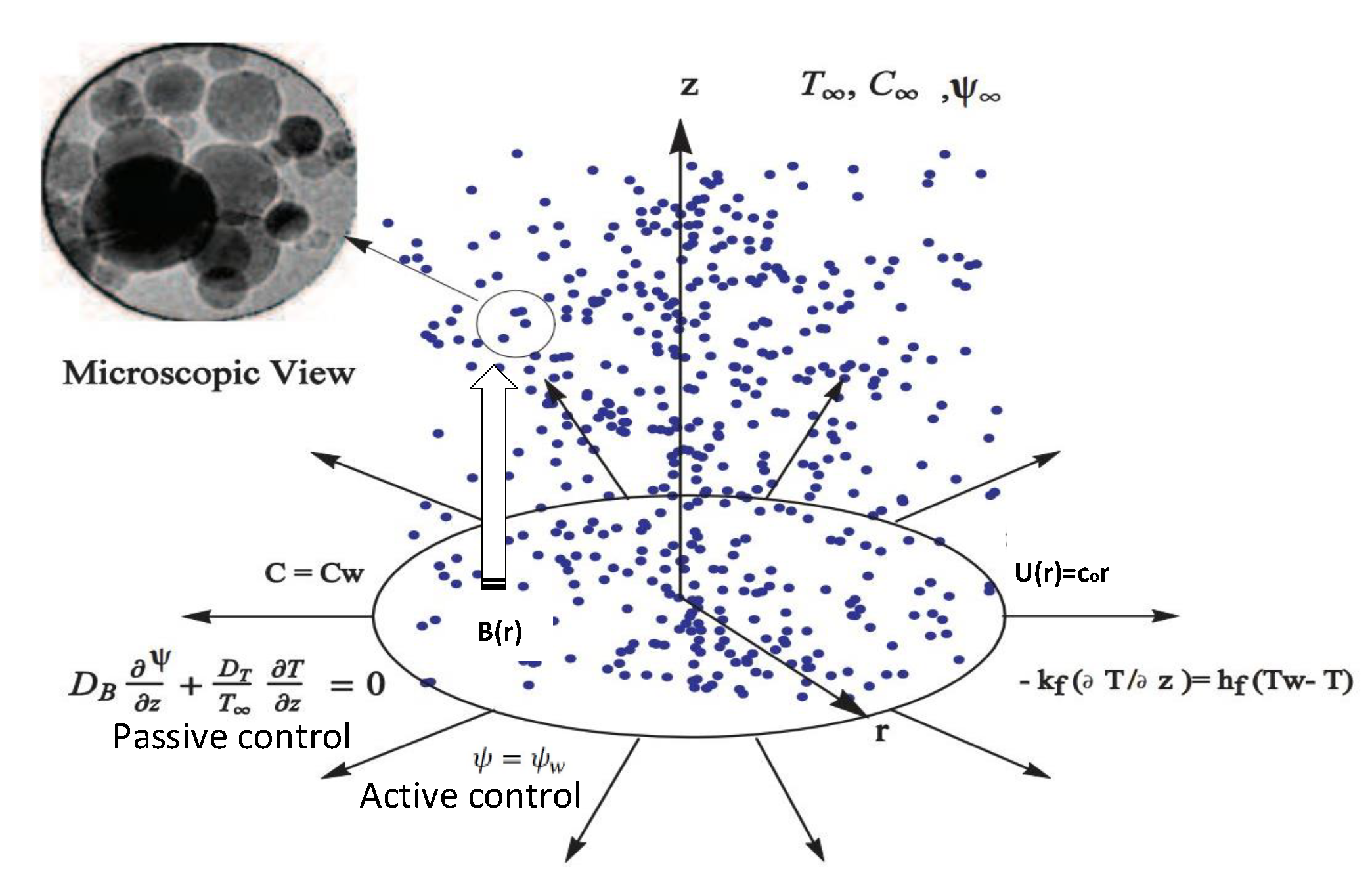
Let us consider a steady magnetohydrodynamic flow of the incompressible viscous flow of a nanofluid over a stretching sheet coinciding with the sheet z = 0 in the presence of a chemical reaction. The flow of the conducting fluid is assumed to be linear along the radial direction U ( r ) = c 0 r , where c 0 is a dimensional constant. The constant temperature, solutal concentration, and nanoparticle concentration are T w , C w , and ψ w respectively. The ambient values of the temperature, solutal concentration, and nanoparticle concentration are denoted by T , C , and ϕ respectively (see Figure 1). It is supposed that the B ( r ) = B o r variable magnetic field intensity acts in z direction, normal to the sheet. Under the above conditions, the governing equations of continuity, momentum conservation, energy conservation, and nanoparticle volume fraction can be expressed as (see [28,29,30]):
u r + u r + w z = 0 ,
u u r + w u z = ν 2 u z 2 σ B 2 ( r ) u ρ
u T r + w T z = α * 2 T z 2 + τ D B ψ z T z + τ D T T ( T z ) 2 + D T C 2 C 2 z
u C r + w C z = D s 2 C z 2 k 1 ( r ) ( C C ) + D C T 2 C 2 z
u ψ r + w ψ z = D B 2 ψ z 2 + D T T 2 T 2 z
The velocity vector of flow is v = v ( u , w ) , where u and w are components of velocity along r and z directions respectively; σ , ν , and ρ are the electrical conductivity, kinetic viscosity, and viscosity of a fluid, respectively; D B and D T , are the Brownian diffusion and thermophoretic diffusion coefficients respectively; D s , D C T , and D T C are the solutal, Soret, and Dufour diffusivities, respectively; and k 1 is the chemical reaction. The corresponding boundary conditions for active control are (see [28,29,31]):
u = U ( r ) + D 1 u z , w = W 0 , κ T z = h f ( T w T ) , C = C w , ψ = ψ w , a t z = 0
u 0 , T , C , ψ , a s z ,
and the corresponding boundary conditions for passive control are (see [11]):
u = U ( r ) + D 1 u z , w = W 0 , κ T z = h f ( T w T ) , C = C w , D B ψ z + D T T T z = 0 , a t z = 0
u 0 , T , C , ψ , a s z ,
where D 1 is the hydrodynamic slip factor and C w is the variable surface concentration.
The following are the similarity transformations to solve the Equations (1)–(5) stated as (see [28,32]):
u = c 0 r f ( ξ ) , ξ = c o ν z , w = c o ν f ( ξ ) , θ ( ξ ) = T T T w T , S ( ξ ) = C C C w C , ϕ ( ξ ) = ψ ψ ψ w ψ
In view of Equation (10), the system of partial differential Equations (2)–(5) transform into the following system of coupled and non-linear ODEs:
d 3 f d ξ 3 + f d 2 f d ξ 2 M d f d ξ d f d ξ 2 = 0 ,
1 P r d 2 θ d ξ 2 d f d ξ θ + f d θ d ξ + T p ( d θ d ξ ) 2 + B m d ϕ d ξ d θ d ξ + D f d 2 S d ξ 2 = 0
1 S c d 2 S d ξ 2 m d f d ξ S + f d S d ξ k c S + S r d 2 θ d ξ 2 = 0
d 2 ϕ d ξ 2 L e d f d ξ ϕ + T p B m d 2 θ d ξ 2 + L e f d ϕ d ξ = 0 ;
the transformed boundary conditions Equations (6) and (7) for active control are:
f ( ξ ) = λ , d f d ξ = 1 + σ f d 2 f d ξ 2 , d θ d ξ = β * [ 1 θ ( ξ ) ] , S ( η ) = 1 , ϕ ( η ) = 1 , a t ξ = 0 ,
d f ( ξ ) d ξ 0 , θ ( ) 0 , S ( ) 0 , ϕ ( ) 0 a t ξ = ;
and the transformed boundary conditions Equations (8) and (9) for passive control are:
f ( ξ ) = λ , d f d ξ = 1 + σ f d 2 f d ξ 2 , d θ d ξ = β * [ 1 θ ( ξ ) ] , S ( η ) = 1 , B m d ϕ d ξ + T p d θ d ξ = 0 , a t ξ = 0 ,
d f ( ξ ) d ξ 0 , θ ( ) 0 , S ( ) 0 , ϕ ( ) 0 a t ξ =
where primes represent differentiation with respect to the variable ξ . The parameters in Equations (11)–(15) are described as:
M = σ B 0 2 ρ c o , P r = κ ρ c p , B m = τ D B ( ψ w ψ ) ν , T p = τ D T ( T w T ) ν T , D f = D T c ( C w C ) ν ( T w T ) , S r = D C T ( T w T ) ν ( C w C ) ,
S c = ν D s , L e = σ D B , β * = ν c 0 c r , k c = k 1 c 0 , λ = W 0 1 c 0 ν
Where M is the magnetic parameter, P r is the Prandtl number, B m is the Brownian motion parameter, T p is the thermophoresis parameter, D f is the Dufour parameter, S r is the Soret parameter, S c is the Schmidt number, L e is the Lewis number, β * is the Biot number, k c is the chemical reaction parameter, σ f is the hydrodynamic slip parameter, and λ represents the mass transfer rate at the surface. λ > 0 is the case for injection and λ < 0 is the case for suction.

3. Finite Element Method (FEM) Solutions

The finite element method was executed on the system of non-linear boundary value problems to acquire the numerical solution that is given in Equations (9)–(12) and was subjected to the boundary conditions of Equations (13) and (14). This method is more adept and reliable than other numerical methods, such as Adomian decomposition method (ADM), homotopy perturbation method (HPM), and finite-difference method (FDM). Additionally, it is very proficient and has been applied to study the miscellaneous problems in fluid mechanics, and in computational fluid dynamics, solid mechanics, mass transfer, heat transfer, and many other fields [33]. Reddy [34] demonstrates an admirable universal feature of the variational finite element method, and confinement in various nonlinear problems, such as simulating the transmission phenomenon of unsteady magnetohydrodynamic [26,35,36] and mixed convection micropolar flow in porous media [37]. In order to apply the finite element method (FEM) to the simultaneous nonlinear differential Equations (9)–(12), and to use the boundary conditions in the Equations (13) and (14), we consider:
d f d ξ = h ,
The set of Equations (9)–(12) thus reduces to
d 2 h d ξ 2 + f d h d ξ M h h 2 = 0 ,
1 P r d 2 θ d ξ 2 h θ + f d θ d ξ + B m d ϕ d ξ d θ d ξ + T p ( d θ d ξ ) 2 + D f d 2 S d ξ 2 = 0 ,
1 S c d 2 S d ξ 2 m h S + f d S d ξ k c S + S r d 2 θ d ξ 2 = 0 ,
d 2 ϕ d ξ 2 L e h ϕ + L e f d ϕ d ξ + T p B m d 2 θ d ξ 2 = 0 ,
The corresponding boundary conditions reduce to following form now for active control:
f ( ξ ) = λ , h ( ξ ) = 1 + σ f d h d ξ , d θ d ξ = β * [ 1 θ ( ξ ) ] , S ( ξ ) = 1 , ϕ ( ξ ) = 1 , a t ξ = 0 ,
h ( ξ ) 0 , θ ( ) 0 , S ( ) 0 , ϕ ( ) 0 a t ξ =
and the corresponding boundary conditions reduce to following form now for passive control:
f ( ξ ) = λ , h ( ξ ) = 1 + σ f d h d ξ , d θ d ξ = β * [ 1 θ ( ξ ) ] , S ( ξ ) = 1 , B m d ϕ d ξ + T p d θ d ξ = 0 , a t ξ = 0 ,
h ( ξ ) 0 , θ ( ) 0 , S ( ) 0 , ϕ ( ) 0 a t ξ =

3.1. Variational Formulations

The weak form connected with Equations (15)–(21) over a linear element Ω a = ( ξ a , ξ a + 1 ) is given by the following.
ξ a ξ a + 1 s 1 { d f d ξ h } d η = 0 ,
ξ a ξ a + 1 s 2 { d 2 h d ξ 2 + f d h d ξ M h h 2 } d ξ = 0 ,
ξ a ξ a + 1 s 3 { 1 P r d 2 θ d ξ 2 h θ + f d θ d ξ + B m d ϕ d ξ d θ d ξ + T p ( d θ d ξ ) 2 + D f d 2 S d ξ 2 } d ξ = 0 ,
ξ a ξ a + 1 s 4 { 1 S c d 2 S d ξ 2 m h S + f d S d ξ k c S + S r d 2 θ d ξ 2 } d ξ = 0 ,
ξ a ξ a + 1 s 5 { d 2 ϕ d ξ 2 L e h ϕ + L e f d ϕ d ξ + T p B m d 2 θ d ξ 2 } d ξ = 0 ,
where s 1 , s 2 , s 3 , s 4 and s 5 are arbitrary test functions.

3.2. Finite Element Formulations

The finite element model may be obtained from Equations (22)–(26) by plugging in the following finite element approximation form.
f ¯ = n = 1 p f ¯ n ψ n , h ¯ = n = 1 p h ¯ n ψ n , d ¯ θ d ξ = n = 1 p d ¯ θ n d ξ ψ n , d ¯ ϕ d ξ = n = 1 p d ¯ ϕ n d ξ ψ n
with s 1 = s 2 = s 3 = s 4 = s 5 = ψ n ( n = 1 , 2 ) , where the test functions ψ n for a typical length element Ω e = ( ξ a , ξ a + 1 ) are given by.
Processes 08 00207 i001
ψ 1 = ξ a + 1 ξ ξ a + 1 ξ a , ψ 2 = ξ ξ a ξ a + 1 ξ a , ξ a ξ ξ a + 1 .
The FE model equations are, therefore, given by.
[ [ A 11 ] [ A 12 ] [ A 13 ] [ A 14 ] [ A 15 ] A 21 ] [ A 22 ] [ A 23 ] [ A 24 ] [ A 25 ] A 31 ] [ A 32 ] [ A 33 ] [ A 34 ] [ A 35 ] A 41 ] [ A 42 ] [ A 43 ] [ A 44 ] [ A 45 ] A 51 ] [ A 52 ] [ A 53 ] [ A 54 ] [ A 55 ] ] [ { f } { h } { θ } { S } { ϕ } ] = [ { b 1 } { b 2 } { b 3 } { b 4 } { b 5 } ]
where [ A m n ] and [ b m ] ( m , n = 1 , 2 , 3 , 4 , 5 ) are the matrices of order 2 × 2 and 2 × 1 , respectively, and all the matrices are given below:
A i j 11 = ξ a ξ a + 1 ψ i d ψ j d ξ d ξ , A i j 12 = ξ a ξ a + 1 ψ i ψ j d ξ , A i j 13 = A i j 14 = 0 , A i j 15 = A i j 21 = 0 ,
A i j 22 = ξ a ξ a + 1 d ψ i d ξ d ψ j d ξ d ξ + ξ a ξ a + 1 f ¯ ψ i d ψ j d ξ d ξ ξ a ξ a + 1 h ¯ ψ i ψ j d ξ M ξ a ξ a + 1 ψ i ψ j d ξ , A i j 23 = 0 , A i j 24 = 0 , A i j 25 = 0 , A i j 31 = 0 , A i j 32 = 0 ,
A i j 33 = 1 P r ξ a ξ a + 1 d ψ i d ξ d ψ j d ξ d ξ ξ a ξ a + 1 h ¯ ψ i ψ j d ξ + ξ a ξ a + 1 f ¯ ψ i d ψ j d ξ d ξ , + B m ξ a ξ a + 1 ϕ ¯ ψ i d ψ j d ξ d ξ + T p ξ a ξ a + 1 θ ¯ ψ i d ψ j d ξ d ξ , A i j 34 = D f ξ a ξ a + 1 d ψ i d ξ d ψ j d ξ d ξ , A i j 35 = 0 , A i j 41 = A i j 42 = 0 , A i j 43 = S r ξ a ξ a + 1 d ψ i d ξ d ψ j d ξ d ξ ,
A i j 44 = 1 S c ξ a ξ a + 1 d ψ i d ξ d ψ j d ξ d ξ + ξ a ξ a + 1 f ¯ ψ i d ψ j d ξ d ξ m ξ a ξ a + 1 h ¯ ψ i ψ j d ξ d ξ k c ξ a ξ a + 1 ψ i ψ j d ξ d ξ , A i j 45 = A i j 51 = A i j 52 = A i j 54 = 0 , A i j 53 = N t N b ξ a ξ a + 1 d ψ i d ξ d ψ j d ξ d ξ
A i j 55 = ξ a ξ a + 1 d ψ i d ξ d ψ j d ξ d ξ + L e ξ a ξ a + 1 f ¯ ψ i d ψ j d ξ d ξ L e ξ a ξ a + 1 h ¯ ψ i ψ j d ξ d ξ ,
and
b i 1 = 0 , b i 2 = ( ψ d h d ξ ) ξ a ξ a + 1 , b i 3 = 1 P r ( ψ d θ d ξ ) ξ a ξ a + 1 d u ( ψ d S d ξ ) ξ a ξ a + 1 , b i 4 = 1 S c ( ψ d S d ξ ) ξ a ξ a + 1 S r ( ψ d θ d ξ ) ξ e ξ e + 1 ,
b i 5 = ( ψ d ϕ d ξ ) ξ a ξ a + 1 T p B m ( ψ d θ d ξ ) ξ e ξ e + 1 ,
where f ¯ = n = 1 2 f ¯ n ψ n , h ¯ = n = 1 2 h ¯ n ψ n , d ¯ θ d ξ = n = 1 2 d ¯ θ n d ξ ψ n and d ¯ ϕ d ξ = n = 1 2 d ¯ ϕ n d ξ ψ n are supposed to be known. The system of equations obtained by Equation (30) is of the order 10 × 10 and the whole flow domain is distributed into 1000 linear elements of the same size. We obtain a matrix after assembly of all element equations. After the assemblage of the system of element equations, an ensuing system of non-linear equations is attained; subsequent to this, it imposes an iterative method to compute it for an effective solution. To compute f ¯ , h ¯ , θ ¯ , and ϕ ¯ , functions are assumed to be known at a lower iteration level to linearize the system. Then, the estimations for the velocity, solutal parameters, nanofluid, temperature, and volume fraction profile are fulfilled for a high level, and continued until the desired accuracy of 0.00005 is not attained. To make sure of the mesh’s independence, the mesh impact ability has been used. There is no considerable disparity in the results observed for ξ > 12 . For that reason, ξ has been fixed at 12. For the corroboration of the convergence of results, we intended for the quantity of elements to enlarge; n = 60 , 100 , 120 , 240 , 260 , 48 , 500 , 700 , 1000 , and 1100. The results are demarcated in Table 1 and Table 2. Additionally, n enhances further than 1000, so no considerable alteration in velocity, temperature, or concentration functions was exposed, so the results of the last outcomes are reported for n = 1000 elements.
As the presented results, an assessment of the fluid velocity has been perceived with the exact solution given by Crane [38] as f ( ξ ) = 1 e x p ( ξ ) with special case ( M = 0 , λ = 0 , σ f = 0 ). The results that have acquired by FEM are a good consensus, which avows the legality of FEM, clearly observed in Table 3. In Table 4, the skin friction coefficient f ( 0 ) obtained by FEM and is also compared with the numerical results of Bagh et al. [39] and exact solution of Mudassar et al. [40], when all other parameters are supposed to be zero. An excellent correlation has been achieved and grid invariance test has been conducted to maintain four decimal point accuracy. In Table 5, the θ ( 0 ) obtained by FEM is also compared with the results of already published articles when remaining parameters are ignored. Our results have decent agreement with the published results that avow the legality of FEM.

4. Results and Discussion

This section was prepared to examine the performance of dimensionless fluid velocity f ( ξ ) , temperature distribution θ ( ξ ) , and concentration profiles ( S ( ξ ) , ϕ ( x i ) ) for active and passive cases, under the effects of various rising entities, such as the magnetic parameter M, Prandtl number P r , Brownian motion B m parameter, thermophoresis parameter T p , Dufour parameter D f , Soret parameter S r , Schmidt number S c , Lewis number L e , Biot number β * , hydrodynamic slip parameter σ f , chemical reaction parameter k c , and suction/injection parameter λ .
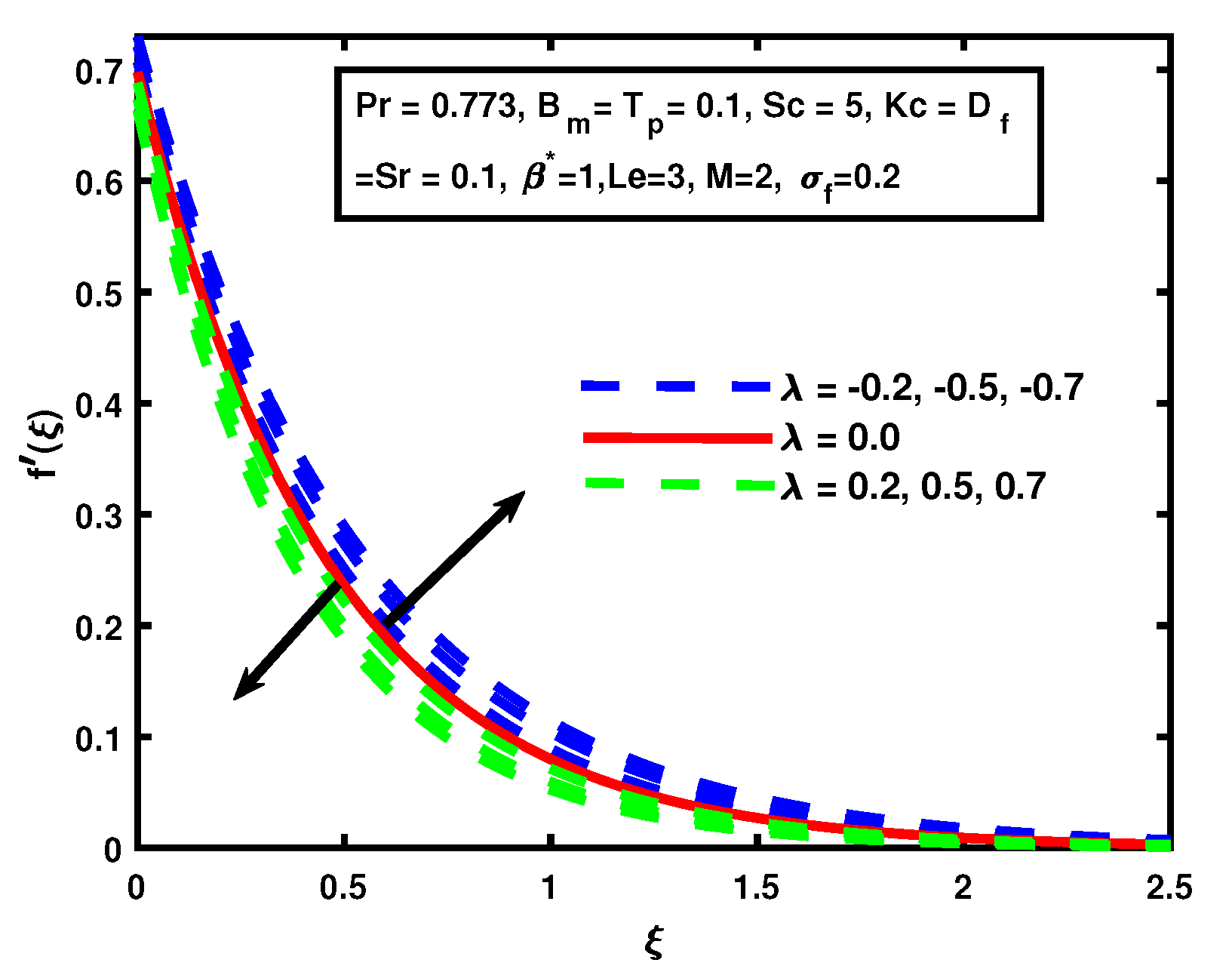
Figure 2 depicts the impact of suction/injection parameter λ . A decline is observed in the velocity function when suction is λ > 0 , and fluid velocity is enhanced for injection λ < 0 . 
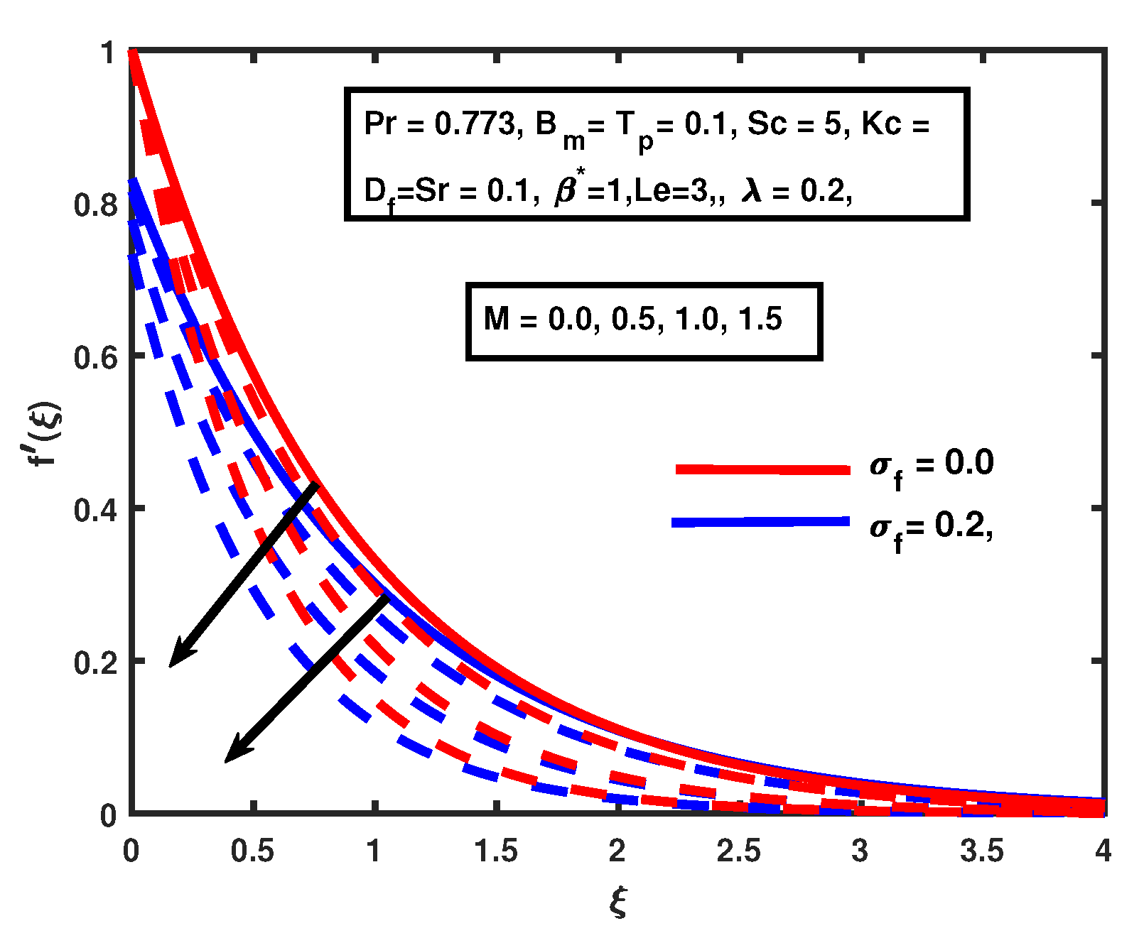
Figure 3 shows the effect of M and hydrodynamic slip σ f on the velocity function. From the consequences, it is discernible that the velocity reduces with the rising values of M. The M-produced Lorentz force slows down the motion of the fluid along the radial direction. The boundary layer thickness can be controlled with the assistance of magnetic M. A similar behavior for velocity has been reported by [28,31]. Additionally, it can be seen in Figure 3 that the velocity of the fluid decreases due to presence of slip.
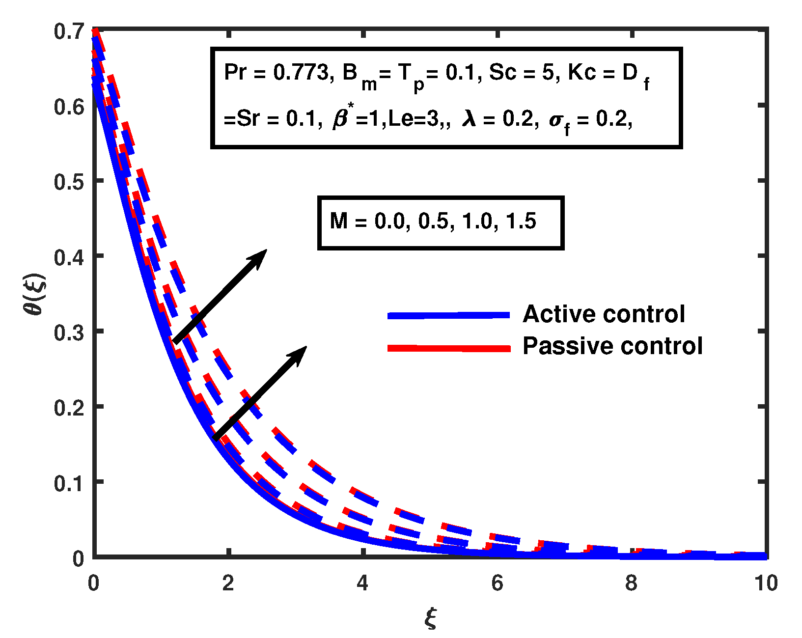
The thickness of the thermal boundary layer increases for different estimations of M. That is clear from Figure 4. The thermal boundary layer;s thickness can also be controlled with the aid of magnetic M. Similar temperature trends have been observed by [31]. The same behavior was observed for both cases: active and passive controls.
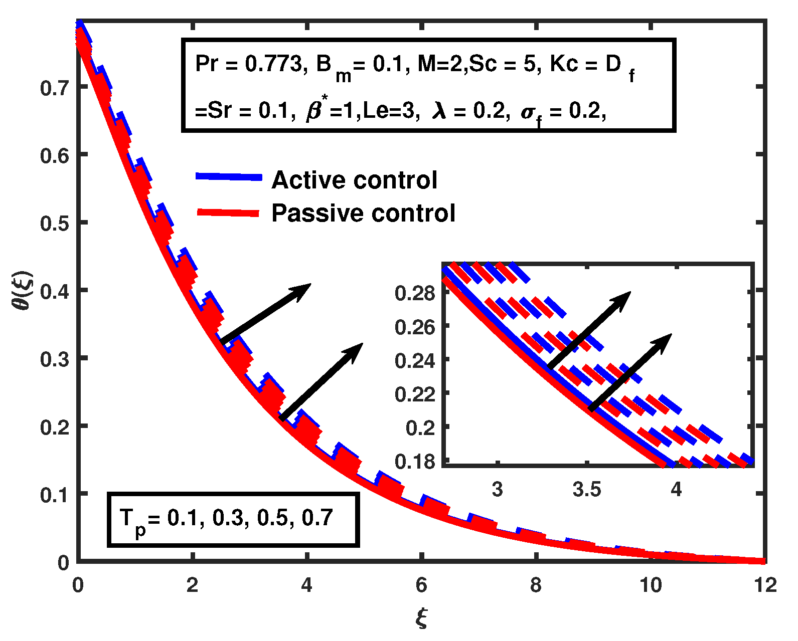
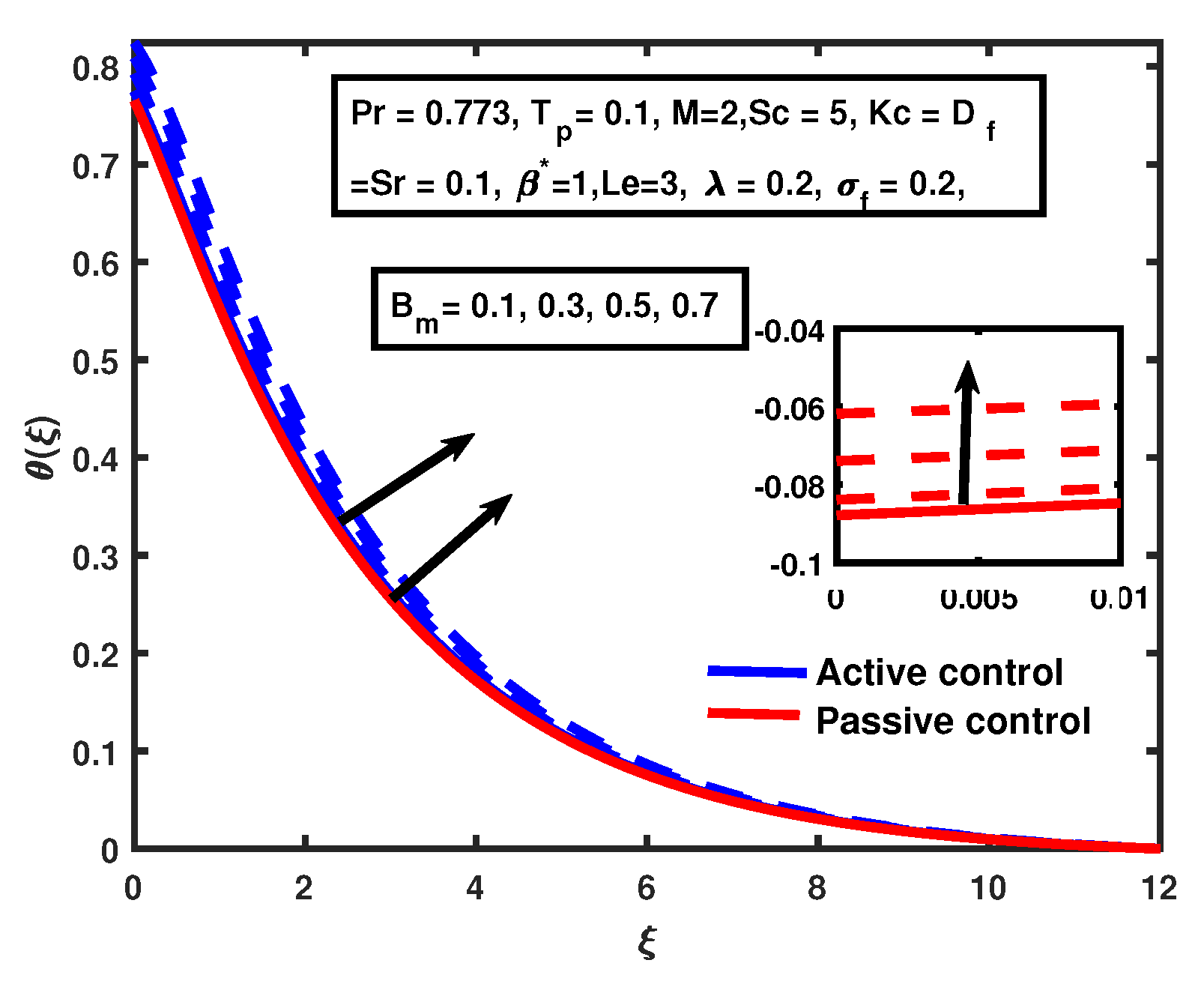
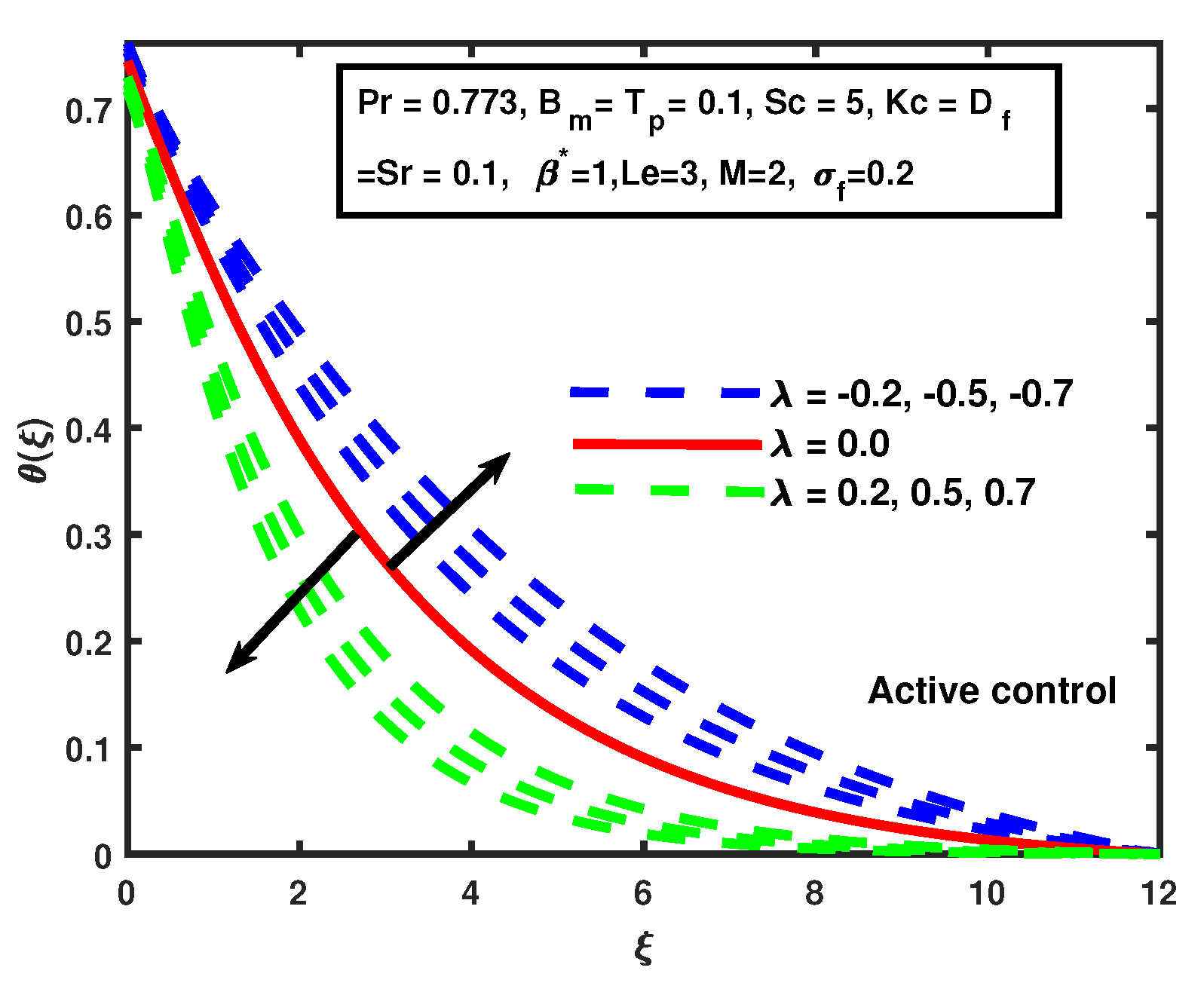
Figure 5 and Figure 6 illustrate that the temperature increases with the enhancement of T p and B m in both cases. A similar trend was reported by [11] for temperature profile. 
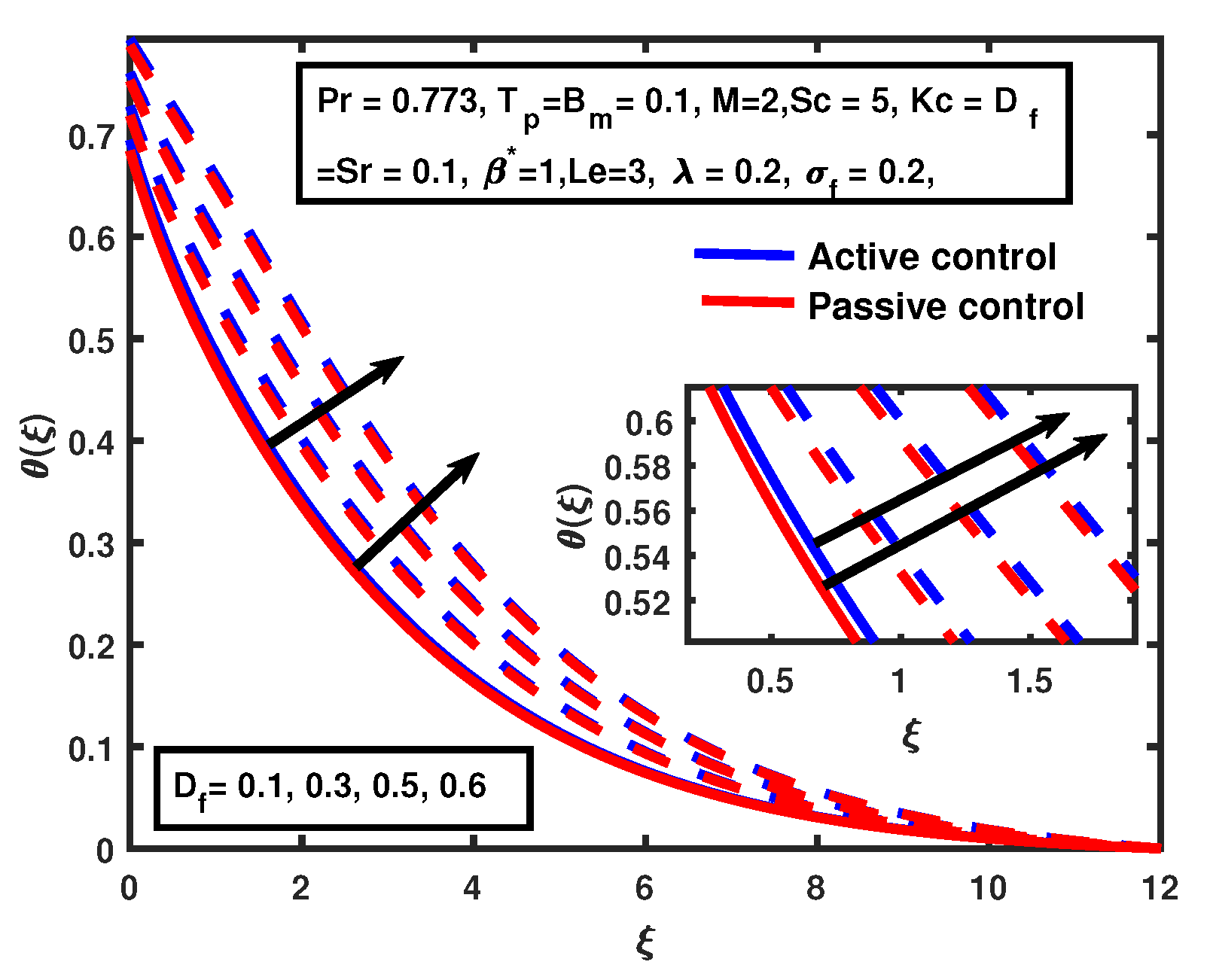
Figure 7 represents the temperature distribution with the variation of the Dufour parameter D f , which shows that the Dufour parameter D f causes an increase in the thickness of the thermal boundary layer. It was also observed that there was no significant variation in active and passive concentration of nanoparticles. 
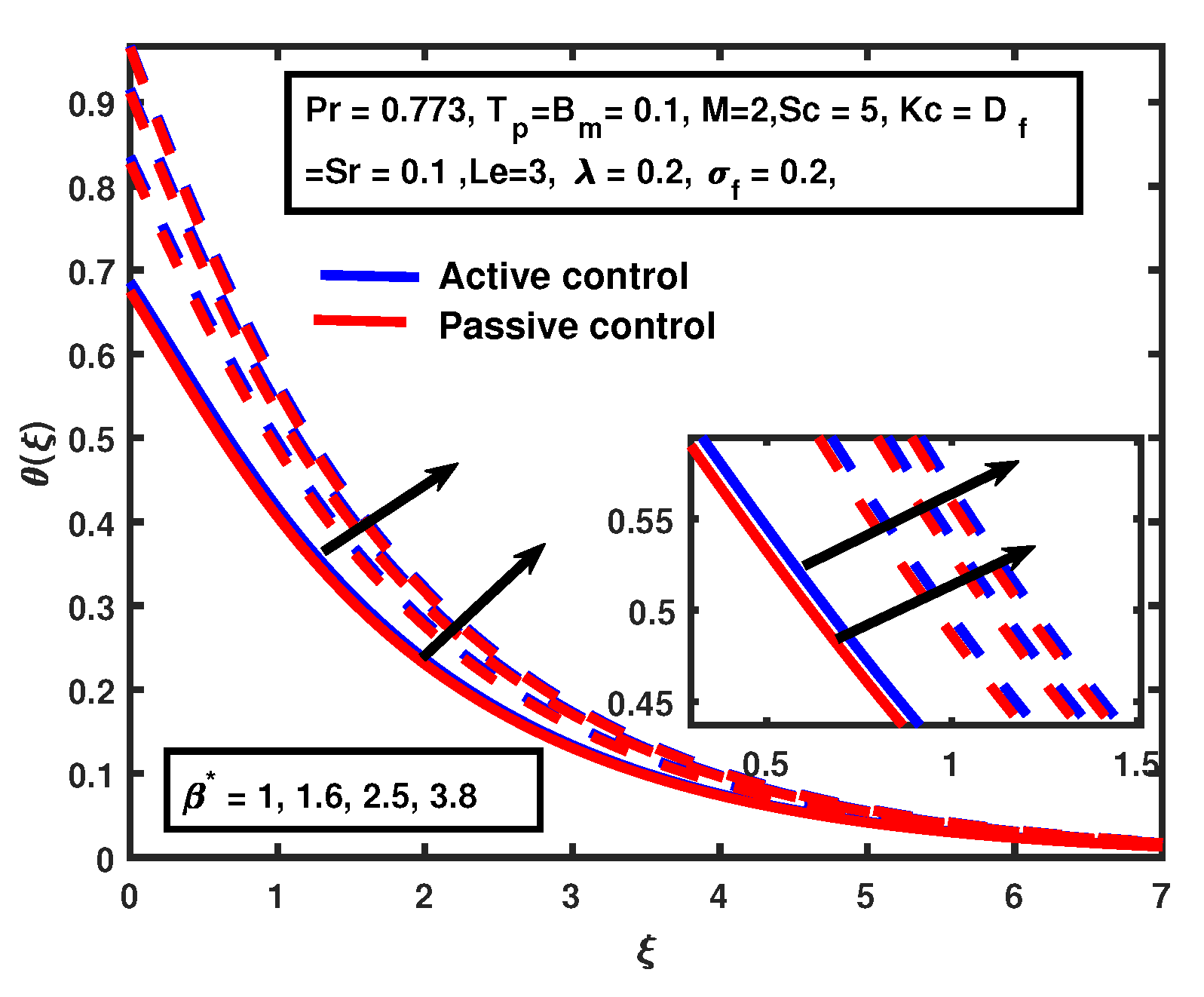
Figure 8 illustrates that the thermal boundary layer thickness increases with the enhancement of β * . The temperature distribution approaches its maximum value at the high value of the Biot number because an increase in β * causes stronger convection. A similar trend for the passive case is noticed.
Figure 9 and Figure 10 depict the establishment of the conversion of the suction/injection parameter λ on the temperature. The injection λ < 0 overshoots the temperature, and opposite behavior of suction λ > 0 is noticed. It is clearly seen in Figure 9 and Figure 10. The similar trend of suction/injection λ for active and passive control cases is seen in Figure 9 and Figure 10. It is also noticed that the impact of λ on the temperature in the active case is greater compared to passive control. The increment in magnetic M causes no significant change in the solutal profile and causes enhancement in the boundary layers of respective solutal profiles for cases of both active and passive control. A similar pattern in the solutal profile has been observed by [28] for the active control case. That is clearly seen in Figure 11.
Figure 12 and Figure 13 demonstrate the impact of suction/injection parameter λ for active and passive control cases. The decline is observed in the solutal function when suction is λ > 0 , and solutal concentration increased for injection λ < 0 . for both cases. The increment in the boundary layer is very fast for the active control case compared to the passive control case when the injection λ < 0 . 
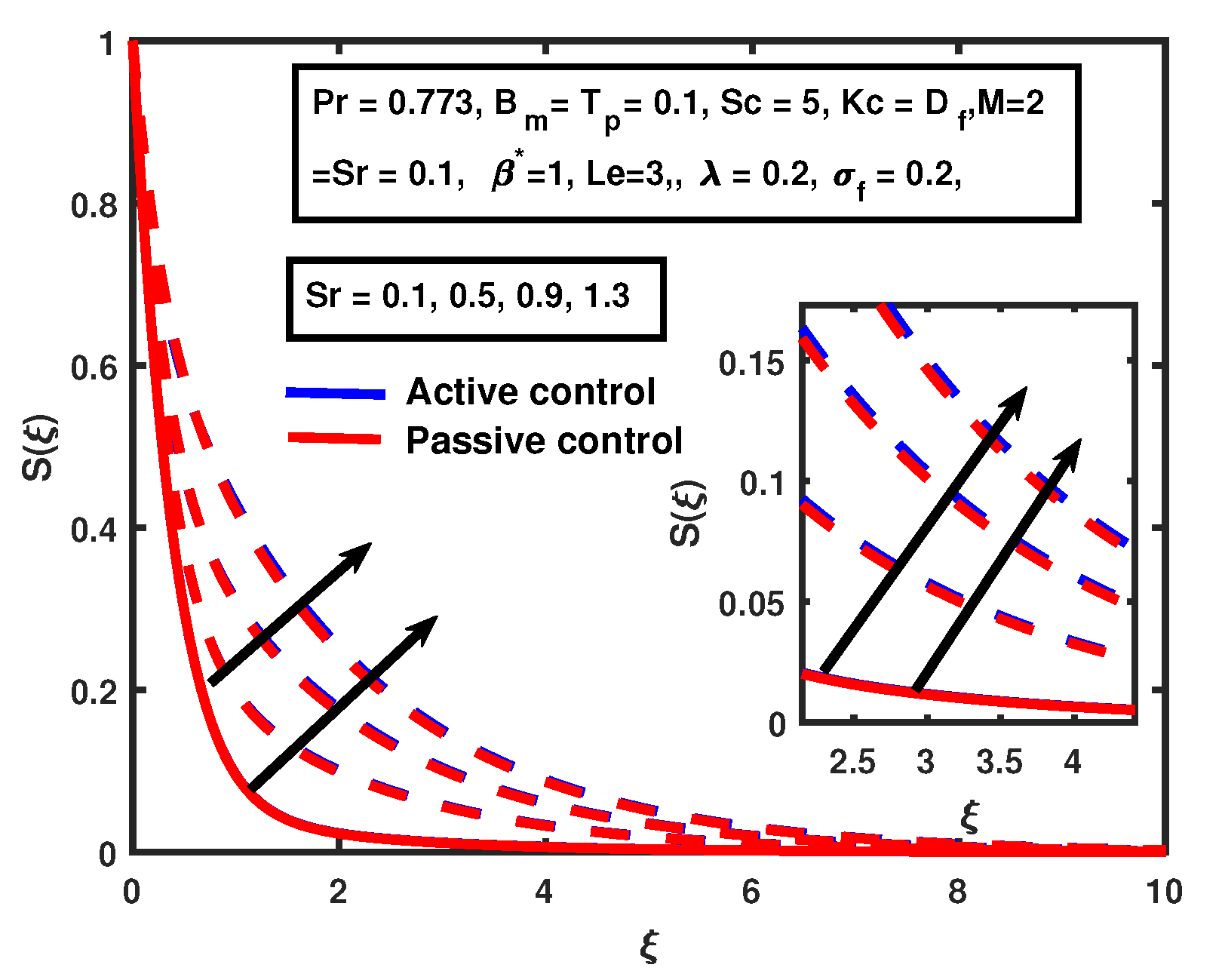
The solutal boundary layer thickness increases as there is an increase of S r for both cases, but there is no significant change between active and passive control. That has been shown in Figure 14.
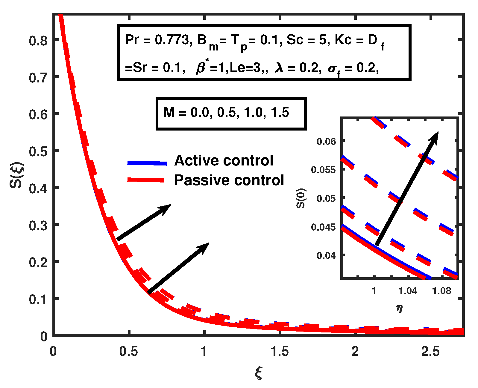
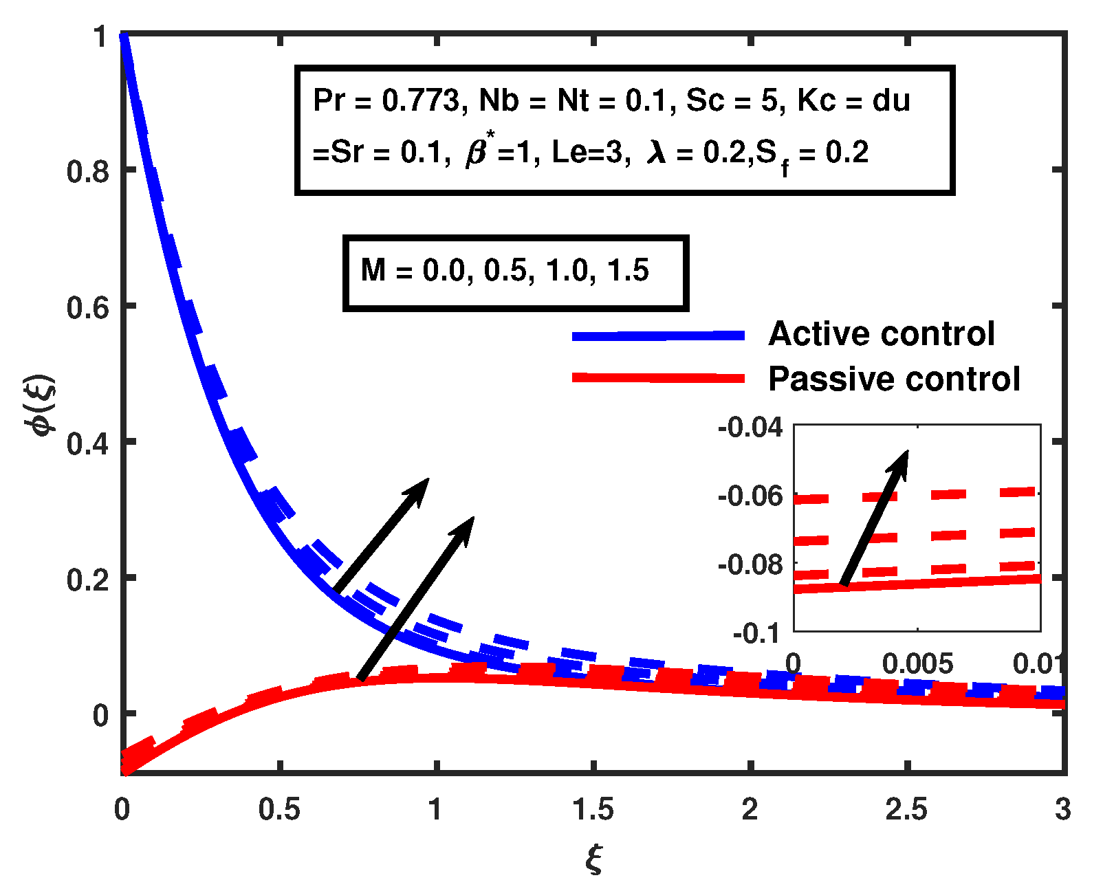
Figure 15 shows the incremental increases in magnetic M caused by increments in the nanoparticle volume fraction profile for cases of both active and passive control. The increment in the boundary layer is very fast for active control case compared to the passive control case when the values of magnetic M are enhanced. Figure 16 and Figure 17 demonstrate the impact of suction/injection parameter λ for active and passive control cases on the nanoparticle volume fraction profile. The decline is observed in the nanoparticle volume fraction profile when suction is λ > 0 , and the nanoparticle volume fraction profile increased for injection λ < 0 . in both cases. Additionally, we observed interesting phenomena for the passive control case: the concentration for ξ 2 . 0 seemed to be increasing when λ > 0 and decreasing for λ < 0 . , and the opposite behavior was noticed for ξ > 2 . 0 . That happens due to zero flux boundary conditions.
The increment in the boundary layer is very fast for the active control case compared to the passive control case when the injection λ < 0 . 
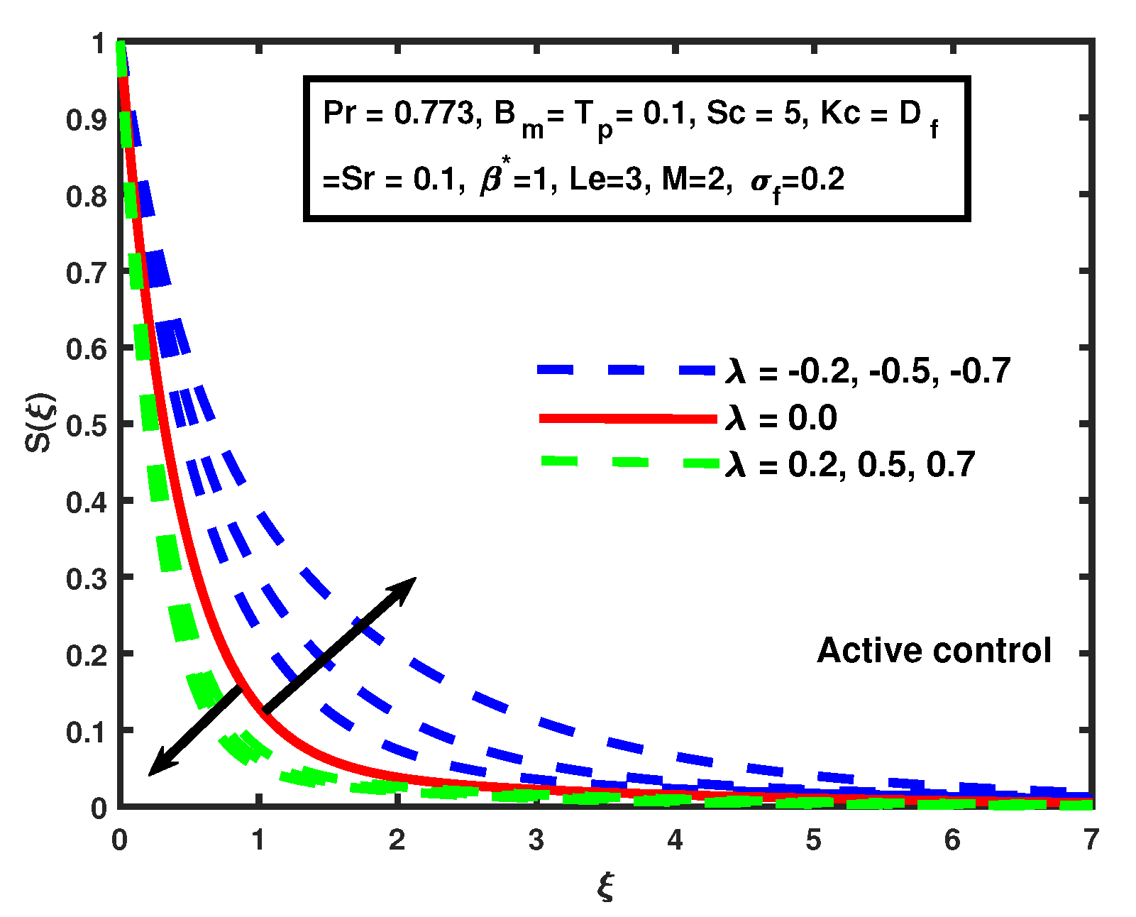
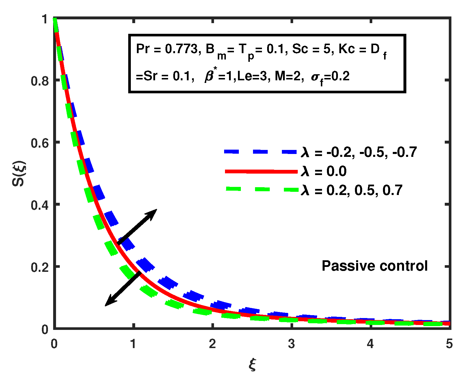
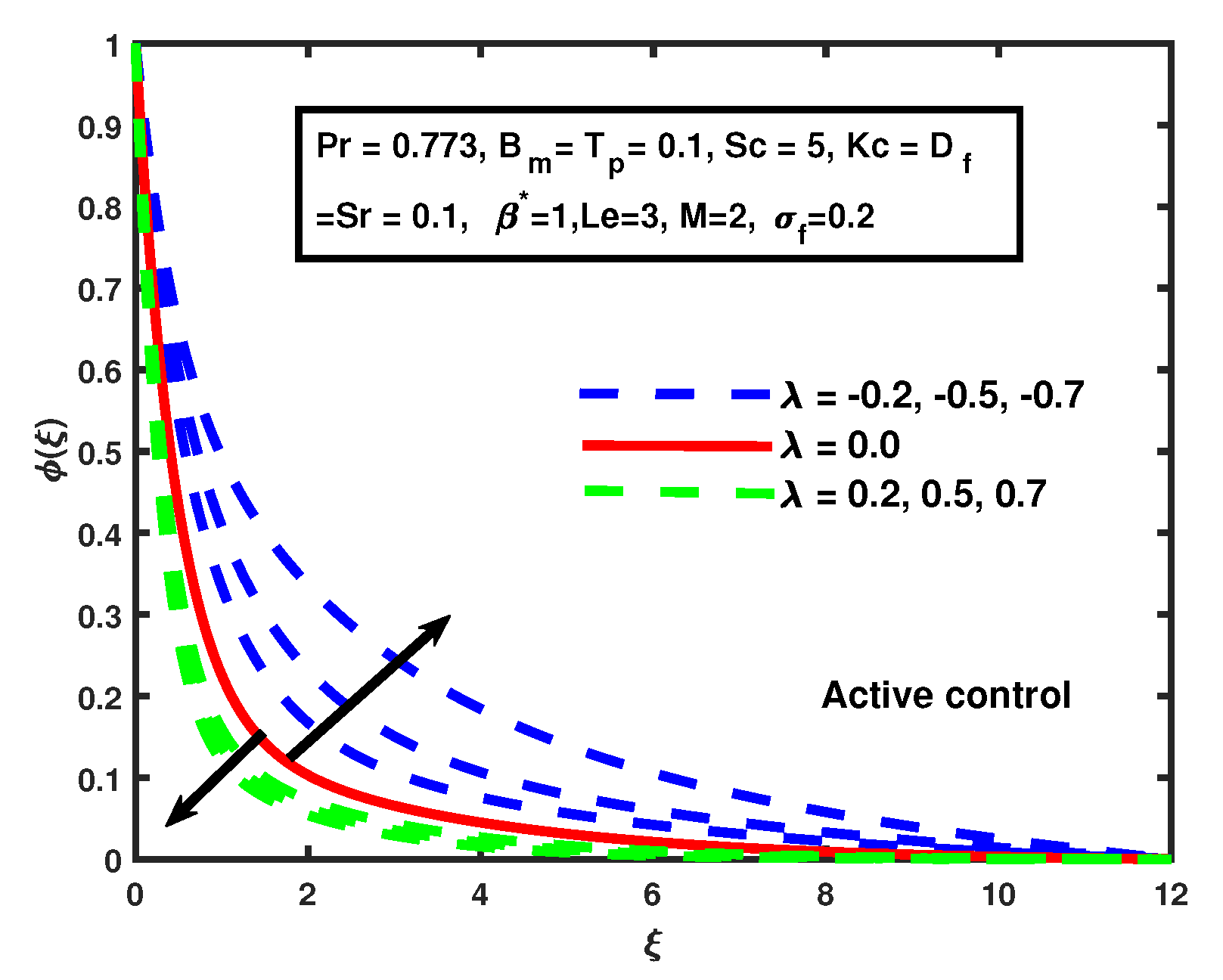
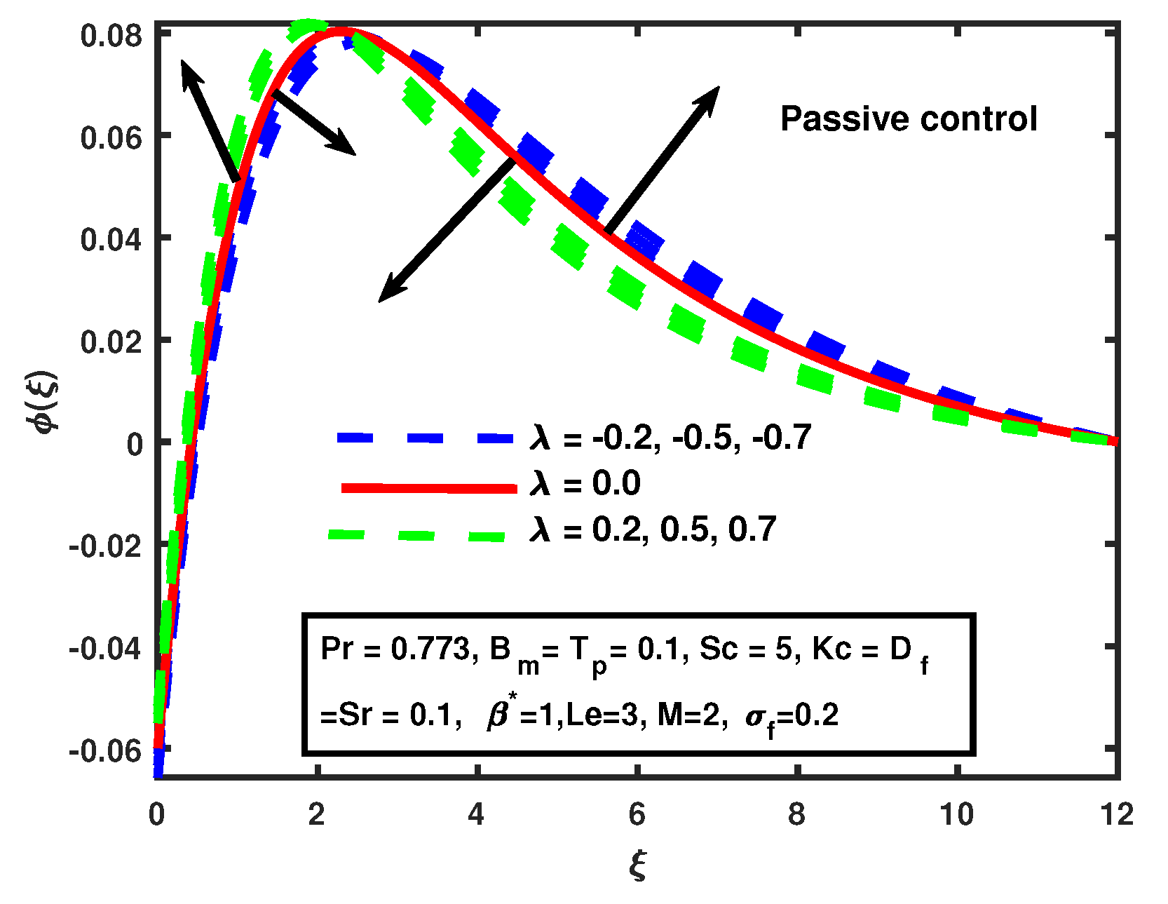
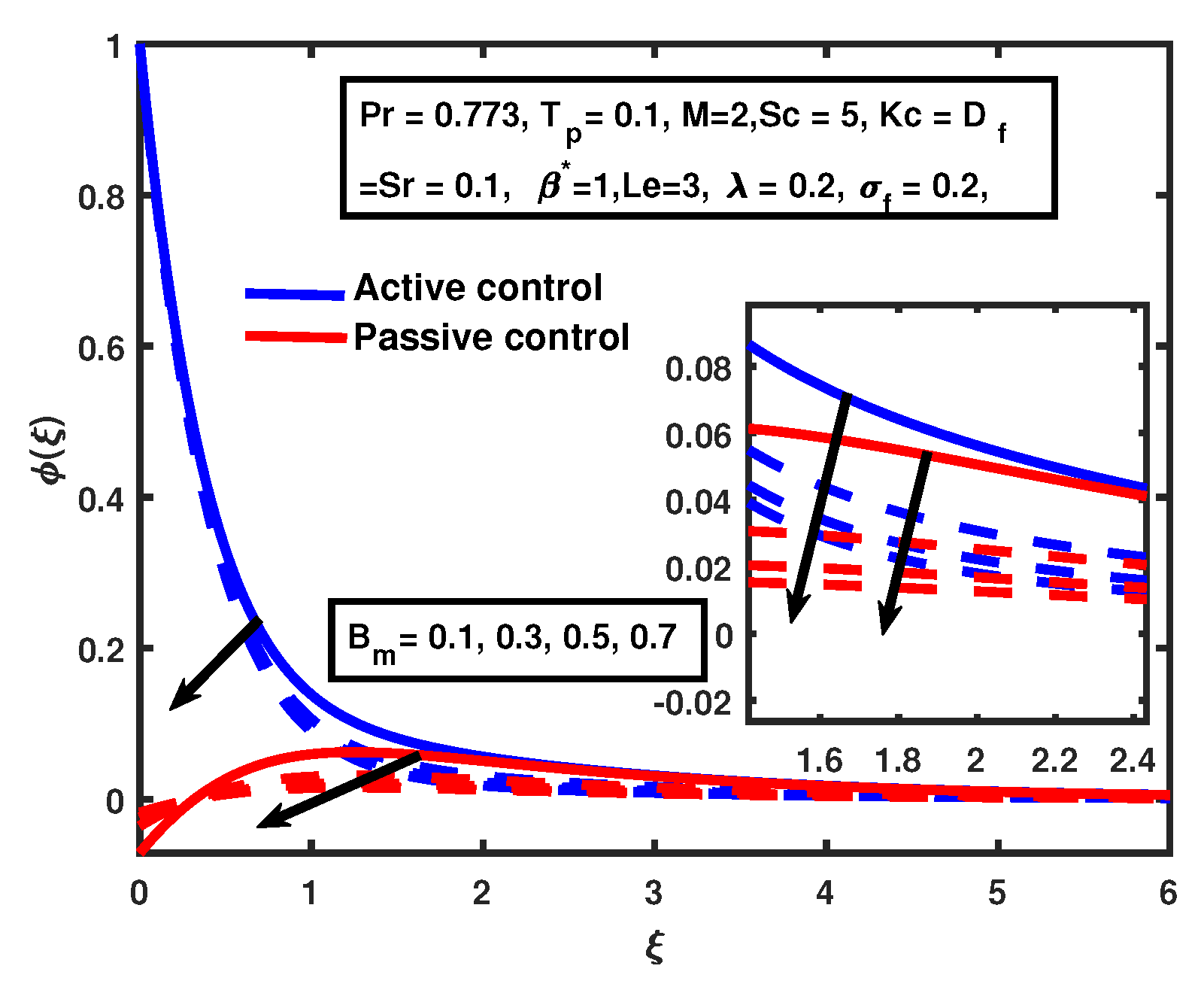
Figure 18 illustrates that the nanoparticle volume fraction profile deceases with the enhancement of B m for both cases, active and passive control, and nanoparticle concentration decreases respectively. A similar trend was reported by [
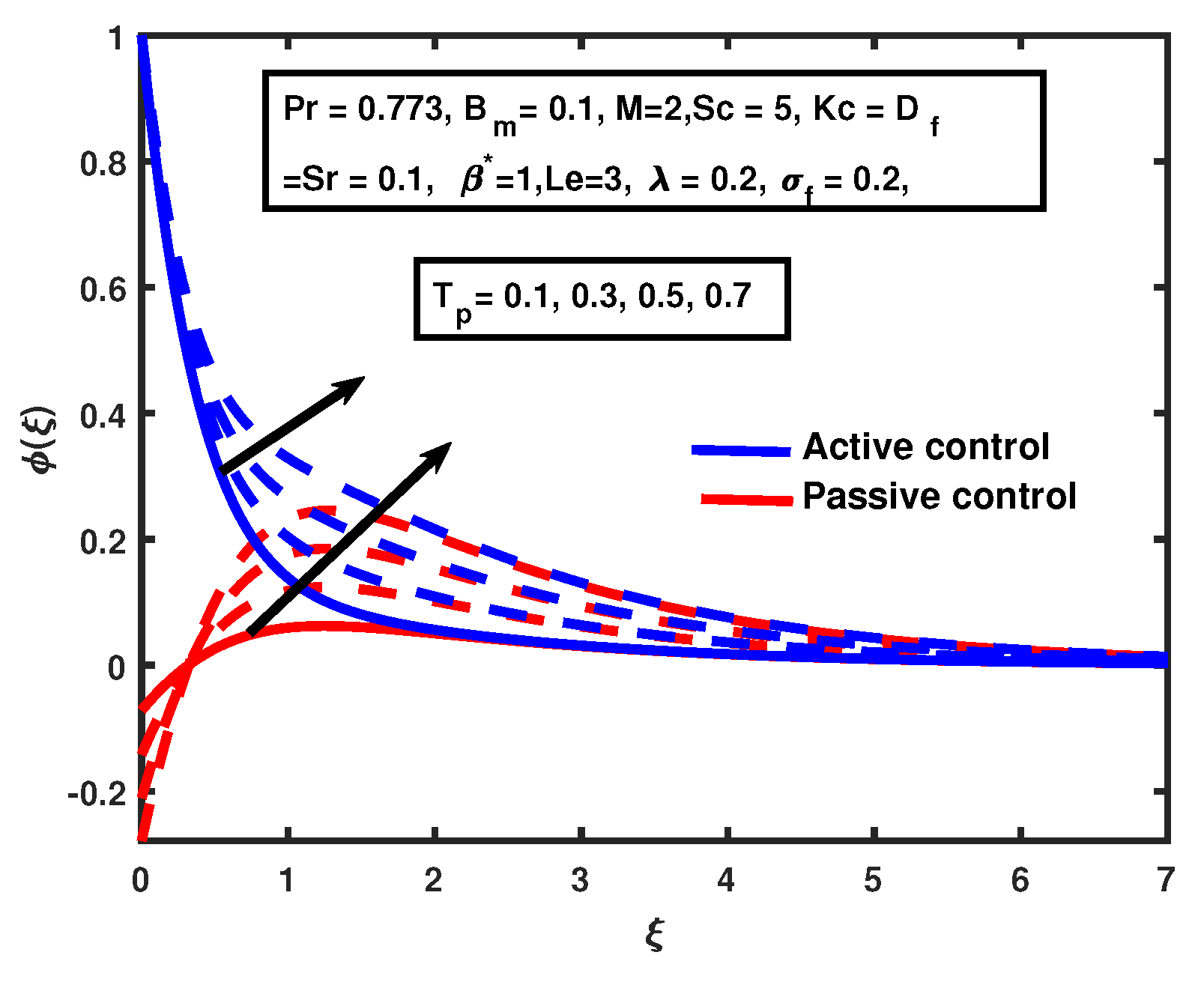
11] for the nanoparticle volume fraction profile for the active control case. An opposite trend was observed with the increment of T p for both cases. Mohyud-Din et al. [11] and Nandy et al. [45] observed a similar trend in the nanoparticle volume fraction profile for the active control case. That is evident from Figure 19.
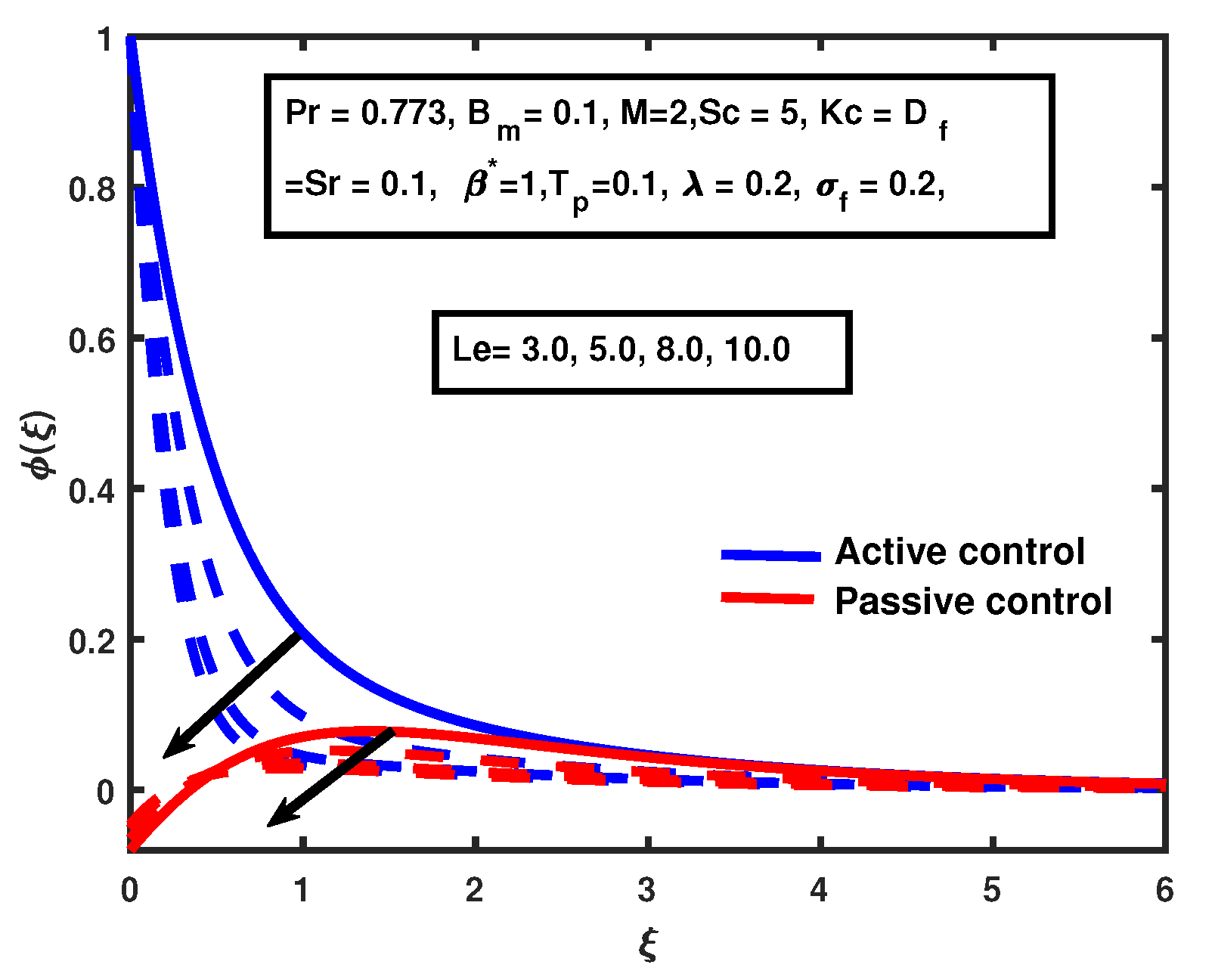
A declining trend has been observed in terms of nanoparticle volume fraction, as it increases L e for both active and passive control cases. That is clear from Figure 20, which shows the decreasing nanofluid volume fraction boundary layer. The passive control gives a more realistic approach to controlling the nanofluid volume fraction boundary layer.
In Table 6 we observe the conversion of physical parameters P r , λ , S c , and β * on the f ( 0 ) , θ ( 0 ) , and ϕ ( 0 ) . The following results are concluded from the Table 6:
(i)
The f ( 0 ) , θ ( 0 ) , and ϕ ( 0 ) increase with a thorough improvement in the increment of λ for both active and passive controls cases.
(ii)
The increment in Prandtl number Pr, causes increasing θ ( 0 ) and ϕ ( 0 ) for both active and passive controls cases.
(iii)
The θ ( 0 ) decreases with the increasing Schmidt number for both cases, and increments in the ϕ ( 0 ) for the active control case, but the opposite trend is observed for the passive control case.
(iv)
The θ ( 0 ) increases with the increment of β * for both cases and declines in ϕ ( 0 ) for the active control case, but the opposite trend is observed for passive control case.

5. Conclusions

Through inspection and discussion, we analyzed the active and passive controls of magnetohydrodynamic an axisymmetric nanofluid flow with a convective boundary condition and thermo-diffusion over a stretched sheet. The considerations for solutal, velocity, temperature, nanoparticle, and volume fraction functions at sundry assessments of physical parameters have been executed. A few stirring expositions from the contemporary work are avowed as:
  • Influence of injection λ < 0 parameter is to proceed with the fluid velocity, fluid temperature, and solutal and nanoparticles concentration functions but opposite behavior is observed for suction λ > 0 for both active and passive controls.
  • Increments in the magnetic field parameter enhance the fluid temperature, and solutal and nanoparticle concentration functions for both active and passive controls, but decline the fluid velocity.
  • The temperature and nanoparticle concentration functions exhibit a similar trend for increasing values of thermophoresis parameter T m in the presence of active and passive controls (both cases). The temperature exhibits similar behavior for greater values of Brownian motion parameter B m , while the opposite trend is observed for nanoparticle concentration functions.
  • The influence of the Dufour parameter and Biot number is to increase the fluid temperature in the presence of active or passive controls.
  • A greater Lewis number ( L e ) suppresses the nanoparticle concentration in the presence of both active and passive controls.
  • The f ( 0 ) parameter exhibits opposite behavior for λ < 0 and λ > 0 . The θ ( 0 ) parameter decreases with increasing Schmidt number for both cases, and increments in ϕ ( 0 ) for the active control case, but the opposite trend is observed for the passive control case.
  • The θ ( 0 ) parameter increases with the increment of β * for both cases, and declines in ϕ ( 0 ) for the active control case, but the opposite trend is observed for the passive control case. The increment in Prandtl number Pr, causes an increase in θ ( 0 ) and ϕ ( 0 ) for both active and passive control cases.
  • The θ ( 0 ) increases with the increment of β * for both cases, and declines in ϕ ( 0 ) for the active control case, but the opposite trend is observed for the passive control case. The increment in Prandtl number Pr causes increasing θ ( 0 ) and ϕ ( 0 ) for both active and passive controls cases.

Author Contributions

B.A. and X.Y. modeled the problem and wrote the manuscript. X.Y. thoroughly checked the mathematical modeling and English. B.A. solved the problem using MATLAB software. Writing—review and editing, M.T.S., L.A., and A.U.R. X.Y. contributed to the results and discussion. All authors finalized the manuscript after its internal evaluation. All authors have read and agreed to the published version of the manuscript.

Funding

This work was supported in part by the Natural Science Basic Research Plan in Shaanxi Province of China (2018JQ6014), the Fundamental Research Funds for the Central Universities (G2018KY0308), the Chinese Postdoctoral Science Foundation (2018M641013) and Postdoctoral Science Foundation of Shaanxi Province (Grant No. 2018BSHYDZZ05).

Conflicts of Interest

The authors declare no conflict of interest.

Nomenclature

MMagnetic parameter
B m Brownian motion parameter
T p Thermo-phoresis parameter
P r Prandtl number
L e Lewis number
D f Dufour parameter
S r Soret parameter
S c Schmidt number
K c Chemical reaction
λ Suction/Injection parameter
σ Electrical conductivity
α * Thermal diffusivity
TTemperature
σ f hydrodynamic slip parameter
β * Biot number
T w Sheet temperature
T Ambient temperature
C w Solutal concentration
C Ambient solutal concentration
U ( x ) Velocity of sheet
ϕ w Nanoparticle volume fraction
D T Thermal diffusivity
D s Molecular diffusivity
D B Brownian diffusivity
D C T Soret diffusivity
D T c Dufour diffusivity
μ Dynamic viscosity
ρ Fluid density
u , v Velocity components
ψ n test functions

References

  1. Aziz, A.; Khan, W.A.; Pop, I. Free convection boundary layer flow past a horizontal flat plate embedded in porous medium filled by nanofluid containing gyrotactic microorganisms. Int. J. Therm. Sci. 2012, 56, 48–57. [Google Scholar] [CrossRef]
  2. Choi, S. Enhancing thermal conductivity of fluids with nanoparticle. In Development and Applications of Non-Newtonian Flow; Argonne National Lab.: DuPage County, IL, USA, 1995; pp. 99–105. [Google Scholar]
  3. Ariel, P.D. Axisymmetric flow of a second grade fluid past a stretching sheet. Int. J. Eng. Sci. 2001, 39, 529–553. [Google Scholar] [CrossRef]
  4. Akbari, O.A.; Safaei, M.R.; Goodarzi, M.; Akbar, N.S.; Zarringhalam, M.; Shabani, G.A.S.; Dahari, M. A modified two-phase mixture model of nanofluid flow and heat transfer in a 3-D curved microtube. Adv. Powder Technol. 2016, 27, 2175–2185. [Google Scholar] [CrossRef]
  5. Abbassi, M.A.; Safaei, M.R.; Djebali, R.; Guedri, K.; Zeghmati, B.; Alrashed, A.A. LBM simulation of free convection in a nanofluid filled incinerator containing a hot block. Int. J. Mech. Sci. 2018, 144, 172–185. [Google Scholar] [CrossRef]
  6. Abdollahzadeh Jamalabadi, M.Y.; Alamian, R.; Yan, W.M.; Li, L.K.; Leveneur, S.; Safdari Shadloo, M. Effects of nanoparticle enhanced lubricant films in thermal design of plain journal bearings at high Reynolds numbers. Symmetry 2019, 11, 1353. [Google Scholar] [CrossRef] [Green Version]
  7. Abdollahzadeh Jamalabadi, M.Y.; Ghasemi, M.; Alamian, R.; Wongwises, S.; Afrand, M.; Shadloo, M.S. Modeling of Subcooled Flow Boiling with Nanoparticles under the Influence of a Magnetic Field. Symmetry 2019, 11, 1275. [Google Scholar] [CrossRef] [Green Version]
  8. Karimipour, A.; Taghipour, A.; Malvandi, A. Developing the laminar MHD forced convection flow of water/FMWNT carbon nanotubes in a microchannel imposed the uniform heat flux. J. Magn. Magn. Mater. 2016, 419, 420–428. [Google Scholar] [CrossRef]
  9. Mustafa, M.; Hayat, T.; Alsaedi, A. Axisymmetric flow of a nanofluid over a radially stretching sheet with convective boundary conditions. Curr. Nanosci. 2012, 8, 328–334. [Google Scholar] [CrossRef]
  10. Akbari, O.A.; Toghraie, D.; Karimipour, A.; Marzban, A.; Ahmadi, G.R. The effect of velocity and dimension of solid nanoparticles on heat transfer in non-Newtonian nanofluid. Phys. E Low-Dimens. Syst. Nanostruct. 2017, 86, 68–75. [Google Scholar] [CrossRef]
  11. Mohyud-Din, S.T.; Khan, U.; Ahmed, N.; Rashidi, M.M. A study of heat and mass transfer on magnetohydrodynamic (MHD) flow of nanoparticles. Propuls. Power Res. 2018, 7, 72–77. [Google Scholar] [CrossRef]
  12. Ashraf, M.; Bashir, S. Numerical simulation of MHD stagnation point flow and heat transfer of a micropolar fluid towards a heated shrinking sheet. Int. J. Numer. Methods Fluids 2012, 69, 384–398. [Google Scholar] [CrossRef]
  13. Afrand, M.; Rostami, S.; Akbari, M.; Wongwises, S.; Esfe, M.H.; Karimipour, A. Effect of induced electric field on magneto-natural convection in a vertical cylindrical annulus filled with liquid potassium. Int. J. Heat Mass Transf. 2015, 90, 418–426. [Google Scholar] [CrossRef]
  14. Raza, J. Thermal radiation and slip effects on magnetohydrodynamic (MHD) stagnation point flow of Casson fluid over a convective stretching sheet. Propuls. Power Res. 2019. [Google Scholar] [CrossRef]
  15. Chen, C.H. Laminar mixed convection adjacent to vertical, continuously stretching sheets. Heat Mass Transf. 1998, 33, 471–476. [Google Scholar] [CrossRef]
  16. Sankara, K.K.; Watson, L.T. Micropolar flow past a stretching sheet. Zeitschrift für Angewandte Mathematik und Physik 1985, 36, 845–853. [Google Scholar] [CrossRef] [Green Version]
  17. Hamza, E. The magnetohydrodynamic squeeze film. J. Tribol. 1988, 110, 375–377. [Google Scholar] [CrossRef]
  18. Rana, P.; Bég, O.A. Mixed convection flow along an inclined permeable plate: Effect of magnetic field, nanolayer conductivity and nanoparticle diameter. Appl. Nanosci. 2015, 5, 569–581. [Google Scholar] [CrossRef] [Green Version]
  19. Thumma, T.; Anwar Bég, O.; Kadir, A. Numerical study of heat source/sink effects on dissipative magnetic nanofluid flow from a non-linear inclined stretching/shrinking sheet. J. Mol. Liq. 2017, 232, 159–173. [Google Scholar] [CrossRef]
  20. Seth, G.S.; Sarkar, S. MHD natural convection heat and mass transfer flow past a time dependent moving vertical plate with ramped temperature in a rotating medium with hall effects, radiation and chemical reaction. J. Mech. 2015, 31, 91–104. [Google Scholar] [CrossRef]
  21. Takhar, H.S.; Agarwal, R.S.; Bhargava, R.; Jain, S. Mixed convection flow of a micropolar fluid over a stretching sheet. Heat Mass Transf. 1998, 34, 213–219. [Google Scholar] [CrossRef]
  22. Khan, S.A.; Nie, Y.; Ali, B. Multiple slip effects on magnetohydrodynamic axisymmetric buoyant nanofluid flow above a stretching sheet with radiation and chemical reaction. Symmetry 2019, 11, 1171. [Google Scholar] [CrossRef] [Green Version]
  23. Faraz, F.; Imran, S.M.; Ali, B.; Haider, S. Thermo-diffusion and multi-slip effect on an axisymmetric Casson flow over a unsteady radially stretching sheet in the presence of chemical reaction. Processes 2019, 7, 851. [Google Scholar] [CrossRef] [Green Version]
  24. Faraz, F.; Haider, S.; Imran, S.M. Study of magneto-hydrodynamics (MHD) impacts on an axisymmetric Casson nanofluid flow and heat transfer over unsteady radially stretching sheet. SN Appl. Sci. 2020, 2, 14. [Google Scholar] [CrossRef] [Green Version]
  25. Mahmoodi, M.; Esfe, M.H.; Akbari, M.; Karimipour, A.; Afrand, M. Magneto-natural convection in square cavities with a source-sink pair on different walls. Int. J. Appl. Electromagn. Mech. 2015, 47, 21–32. [Google Scholar] [CrossRef] [Green Version]
  26. Ali, L.; Liu, X.; Ali, B.; Mujeed, S.; Abdal, S. Finite Element Analysis of Thermo-Diffusion and Multi-Slip Effects on MHD Unsteady Flow of Casson Nano-Fluid over a Shrinking/Stretching Sheet with Radiation and Heat Source. Appl. Sci. 2019, 9, 5217. [Google Scholar] [CrossRef] [Green Version]
  27. Kumar, L. Finite-element analysis of transient heat and mass transfer in microstructural boundary layer flow from a porous stretching sheet. Comput. Therm. Sci. Int. J. 2014. [Google Scholar] [CrossRef]
  28. Nayak, B.; Mishra, S.R.; Krishna, G.G. Chemical reaction effect of an axisymmetric flow over radially stretched sheet. Propuls. Power Res. 2019, 1–6. [Google Scholar] [CrossRef]
  29. Shahzad, A.; Ahmed, J.; Khan, M. On heat transfer analysis of axisymmetric flow of viscous fluid over a nonlinear radially stretching sheet. Alex. Eng. J. 2016, 55, 2423–2429. [Google Scholar] [CrossRef] [Green Version]
  30. Sajid, M.; Hayat, T.; Asghar, S.; Vajravelu, K. Analytic solution for axisymmetric flow over a nonlinearly stretching sheet. Arch. Appl. Mech. 2008, 78, 127–134. [Google Scholar] [CrossRef]
  31. Khan, M.; Malik, R.; Munir, A.; Shahzad, A. MHD flow and heat transfer of Sisko fluid over a radially stretching sheet with convective boundary conditions. J. Braz. Soc. Mech. Sci. Eng. 2016, 38, 1279–1289. [Google Scholar] [CrossRef]
  32. Shahzad, A.; Ali, R.; Hussain, M.; Kamran, M. Unsteady axisymmetric flow and heat transfer over time-dependent radially stretching sheet. Alex. Eng. J. 2017, 56, 35–41. [Google Scholar] [CrossRef] [Green Version]
  33. Singh, B.; Gupta, D.; Kumar, L.; Anwar, O.B. Finite Element Analysis of MHD Flow of Micropolar Fluid over a Shrinking Sheet with a Convective Surface Boundary Condition. J. Eng. Thermophys. 2018, 27, 202–203. [Google Scholar] [CrossRef]
  34. Reddy, J.N. Solutions Manual for an Introduction to the Finite Element Method; McGraw-Hill: New York, NY, USA, 1993; pp. 1–41. [Google Scholar]
  35. Rana, P.; Bhargava, R.; Bég, O.A. Finite element simulation of unsteady magneto-hydrodynamic transport phenomena on a stretching sheet in a rotating nanofluid. Proc. Inst. Mech. Eng. Part N J. Nanoeng. Nanosyst. 2013, 227, 77–99. [Google Scholar] [CrossRef]
  36. Ali, L.; Liu, X.; Ali, B.; Mujeed, S.; Abdal, S. Finite Element Simulation of Multi-Slip Effects on Unsteady MHD Bioconvective Micropolar nanofluid Flow Over a Sheet with Solutal and Thermal Convective Boundary Conditions. Coatings 2019, 9, 842. [Google Scholar] [CrossRef]
  37. Bhargava, R.; Rana, P. Finite element solution to mixed convection in MHD flow of micropolar fluid along a moving vertical cylinder with variable conductivity. Int. J. Appl. Math Mech. 2011, 7, 29–51. [Google Scholar]
  38. Crane, L.J. Flow past a stretching plate. Zeitschrift für Angewandte Mathematik und Physik ZAMP 1970, 21, 645–647. [Google Scholar] [CrossRef]
  39. Ali, B.; Nie, Y.; Khan, S.A.; Sadiq, M.T.; Tariq, M. Finite Element Simulation of Multiple Slip Effects on MHD Unsteady Maxwell Nanofluid Flow over a Permeable Stretching Sheet with Radiation and Thermo-Diffusion in the Presence of Chemical Reaction. Processes 2019, 7, 628. [Google Scholar] [CrossRef] [Green Version]
  40. Jalil, M.; Asghar, S.; Yasmeen, S. An Exact Solution of MHD Boundary Layer Flow of Dusty Fluid over a Stretching Surface. Math. Probl. Eng. 2017, 2017, 1–5. [Google Scholar] [CrossRef] [Green Version]
  41. Ishak, A.; Nazar, R.; Pop, I. Boundary layer flow and heat transfer over an unsteady stretching vertical surface. Meccanica 2009, 44, 369–375. [Google Scholar] [CrossRef]
  42. Mabood, F.; Shateyi, S. Multiple slip effects on MHD unsteady flow heat and mass transfer impinging on permeable stretching sheet with radiation. Model. Simul. Eng. 2019, 2019, 3052790. [Google Scholar] [CrossRef] [Green Version]
  43. Pal, D. Combined effects of non-uniform heat source/sink and thermal radiation on heat transfer over an unsteady stretching permeable surface. Commun. Nonlinear Sci. Numer. Simul. 2011, 16, 1890–1904. [Google Scholar] [CrossRef]
  44. Haile, E.; Shankar, B. Heat and Mass Transfer in the Boundary Layer of Unsteady Viscous Nanofluid along a Vertical Stretching Sheet. J. Comput. Eng. 2014, 2014, 1–17. [Google Scholar] [CrossRef] [Green Version]
  45. Nandy, S.K.; Mahapatra, T.R. Effects of slip and heat generation/absorption on MHD stagnation flow of nanofluid past a stretching/shrinking surface with convective boundary conditions. Int. J. Heat Mass Transf. 2013, 64, 1091–1100. [Google Scholar] [CrossRef]
Figure 1. Physical configuration and coordinate system.
Processes 08 00207 g001
Figure 2. The impact of f ( ξ ) on suction/injection λ .
Processes 08 00207 g002
Figure 3. The impact of f ( ξ ) on magnetic M and hydrodynamic slip σ f .
Processes 08 00207 g003
Figure 4. The impact of θ ( ξ ) on magnetic M.
Processes 08 00207 g004
Figure 5. The impact of θ ( ξ ) on thermophoresis T p .
Processes 08 00207 g005
Figure 6. The impact of θ ( ξ ) on Brownian motion B m .
Processes 08 00207 g006
Figure 7. The impact of θ ( ξ ) on Dufour D f .
Processes 08 00207 g007
Figure 8. The impact of θ ( ξ ) on Biot number β * .
Processes 08 00207 g008
Figure 9. The impact of θ ( ξ ) on suction/injection λ (active control case).
Processes 08 00207 g009
Figure 10. The impact of θ ( ξ ) on suction/injection λ (passive control case).
Processes 08 00207 g010
Figure 11. The impact of S ( ξ ) on magnetic M.
Processes 08 00207 g011
Figure 12. The impact of S ( ξ ) on suction/injection λ (active control case).
Processes 08 00207 g012
Figure 13. The impact of S ( ξ ) on suction/injection λ (passive control case).
Processes 08 00207 g013
Figure 14. The impact of S ( ξ ) on Soret S r .
Processes 08 00207 g014
Figure 15. The impact of ϕ ( ξ ) on magnetic M.
Processes 08 00207 g015
Figure 16. The impact of ϕ ( ξ ) on suction/injection λ (active control case).
Processes 08 00207 g016
Figure 17. The impact of ϕ ( ξ ) on suction/injection λ (passive control case).
Processes 08 00207 g017
Figure 18. The impact of ϕ ( ξ ) on Brownian motion B m .
Processes 08 00207 g018
Figure 19. The impact of ϕ ( ξ ) on thermophoresis T p .
Processes 08 00207 g019
Figure 20. The impact of ϕ ( ξ ) on Lewis number L e .
Processes 08 00207 g020
Table 1. FEM convergence results for active control of nanoparticles when P r = 0.773 ; M = 2 ; B m = T p = 0.1 , S c = 5 , k c = D f = S r = 0.1 ; L e = 4 ; m = β * = 1 , λ = 0.2 , and σ f = 0.2 .
Number of Elements f ( 3.0 ) h ( 3.0 ) θ ( 3.0 ) S ( 3.0 ) ϕ ( 3.0 )
600.499780.000730.021270.263240.06208
1000.501880.000750.021220.262060.06185
2600.502900.000760.021190.261480.06173
5000.503030.000760.021190.261410.06172
7000.503060.000760.021190.261400.06172
10000.503070.000760.021190.261390.06171
11000.503070.000760.021190.261390.06171
Table 2. FEM convergence results for passive control of nanoparticles when P r = 0.773 ; M = 2 ; B m = T p = 0.1 , S c = 5 , k c = D f = S r = 0.1 ; L e = 4 ; m = β * = 1 , λ = 0.2 , and σ f = 0.2 .
Number of Elements f ( 3.0 ) h ( 3.0 ) θ ( 3.0 ) S ( 3.0 ) ϕ ( 3.0 )
600.495750.000660.020950.259850.05915
1200.502250.000750.020790.256270.05824
2400.502870.000760.020780.255920.05815
4800.503030.000760.020770.255840.05813
7000.503060.000760.020770.255820.05812
10000.503070.000760.020770.255810.05812
11000.503070.000760.020770.255810.05812
Table 3. Comparison of the f ( η ) with the published results of Crane [38].
ξ   [38]FEMError in % ξ   [38]FEMError in %
(a) Exact Solution(b) (Our Results) | ( b a a ) | × 100 (a) Exact Solution(b) (Current Results) | ( b a a ) | × 100
0.01.00001.000000.000005.00.00670.006700.00000
1.00.13790.137870.021756.00.00250.002510.40000
2.00.13530.135340.029567.00.00090.000911.11111
3.00.04980.049760.080328.00.00030.000313.33333
4.00.01830.018330.163939.00.00010.0001110.0000
Table 4. The coefficient of skin friction in comparison with different values of magnetic parameter M.
MBagh et al. [39]Mudassar et al. [40]FEM (Our Results)Error in %
Exact Solution (a)(b) | ( b a a ) | × 100
0.01.00001.0000001.00000800.00080
0.21.09541.0954451.09544580.00007
0.51.22471.2247451.22474460.00003
1.01.41421.4142141.41421320.00006
1.21.48321.4832401.48323930.00005
1.51.58111.5811391.58113840.00004
2.01.73211.7320511.73205040.00003
Table 5. Assessment of θ ( 0 ) for numerous values of P r when β * .
PrFazle et al.Dulal Pal.Haile et al.Ishak et al.  [41]FEMError in %
[42][43][44](a) Accurate Solution(b) (Current Results) | ( b a a ) | × 100
0.720.8088--0.80863134980.80863392890.0003
1.001.00001.00001.00041.0000000001.00000802100.0008
3.001.92371.92361.92341.9236825941.92367772230.0003
10.03.72073.72073.72053.7206739013.72066816850.0002
100-12.294012.296212.29408326012.2940516610.0003
Table 6. Assessment of f ( 0 ) , θ ( 0 ) , and ϕ ( 0 ) for numerous values of Pr and Sc ( M = 1 ; N b = 0.1 ; N t = 0.1 ; S c = 4 ; s i g m a = 0.1 ; L e = 4 ; D f = 0.1 ; S r = 0.1 ; N = 1 ; B i = 1 ; S = 0.2 ; S f = 0.2 ; b b = 1 ).
PrSc λ β * Active ControlPassive Control
f ( 0 ) , θ ( 0 ) , ϕ ( 0 ) f ( 0 ) θ ( 0 ) ϕ ( 0 )
0.7734.00.21.01.1160360.3142702.2303581.1160360.325653−0.325653
1.000 1.1160360.3379022.2380651.1160360.353987−0.353987
2.000 1.1160360.3691812.3045431.1160360.406317−0.406317
0.7734.00.21.01.1160360.3142702.2303581.1160360.325653−0.325653
5.0 1.1160360.2969122.2485321.1160360.308299−0.308299
7.0 1.1160360.2641452.2844241.1160360.275669−0.275669
0.7734.00.21.01.1160360.3142702.2303581.1160360.325653−0.325653
0.5 1.2116340.3280793.0473081.2116340.340621−0.340621
0.7 1.2777550.3367873.6513591.2777550.349912−0.349912
0.7734.00.21.01.1160360.3142702.2303581.1160360.325653−0.325653
2.01.1160360.3919652.1901851.1160360.409853−0.409853
3.01.1160360.4270542.1720551.1160360.448419−0.448419

