Abstract
Microalgae can be raw materials for the production of clean energy and have great potential for development. The design of the microalgal photobioreactor (PBR) affects the mixing of the algal suspension and the utilization efficiency of the light energy, thereby affecting the high-efficiency cultivation of the microalgae. In this study, a spiral rib structure was introduced into a tubular microalgal PBR to improve the mixing performance and the light utilization efficiency. The number of spiral ribs, the inclination angle, and the velocity of the algal suspension were optimized for single-sided and double-sided parallel light illuminations with the same total incident light intensity. Next, the optimization results under the two illumination modes were compared. The results showed that the double-sided illumination did not increase the average light/dark (L/D) cycle frequency of the microalgae particles, but it reduced the efficiency of the L/D cycle enhancement. This outcome was analyzed from the point of view of the relative position between the L/D boundary and the vortex in the flow field. Finally, a method to increase the average L/D cycle frequency was proposed and validated. In this method, the relative position between the L/D boundary and the vortex was adjusted so that the L/D boundary passed through the central region of the vortex. This method can also be applied to the design of other types of PBRs to increase the average L/D cycle frequency.
1. Introduction
Energy and environmental issues are a serious concern in the contemporary world. The consumption of conventional fossil fuels has brought not only air pollution, but also an impending energy crisis. Microalgae are coming into view because of their vast potential for substituting for traditional fossil fuels. Many species of algae accumulate carbohydrates during their growth from which ethanol can be produced by the microorganisms’ anaerobic fermentation [1]. Ethanol mixed with gasoline, named biogasoline, is used as an automotive fuel. As oil microorganisms, certain algae have an advantage in their ability for oil production over oil crops such as the coconut and the Jatropha curcas, reaching 700 gallon per hectare while 285 gallon for the coconut and 201 for the Jatropha curcas [2]. Recently, an efficient way to generate methane from whole algae biomass was published with conversion efficiency of 84% [3,4]. In the environmental industry, microalgae can play a vital role; they can absorb carbon dioxide from waste gas as inorganic carbon and inorganic substances from contaminated water as nutrients [5], which would relieve green-house gas emission and water pollution to some degree.
However, the productivity of microalgae is limited under natural conditions and cannot meet the demand for high-efficiency production. Therefore, increasing the productivity of microalgae has become an urgent problem that must be solved. There are two ways to increase the productivity of microalgae. The first is by changing the microalgae itself, such as mutagenesis [6,7,8,9], and screening out high-quality microalgae, and the second is by providing suitable growth conditions for the microalgae, such as designing a suitable photobioreactor (PBR) for microalgae culture. PBRs are available in both enclosed and open configurations. Open PBRs include raceway ponds and circular ponds, where raceway ponds are commonly used open PBRs. The advantage of raceway pond PBRs is that they can culture a large amount of algae at one time and have a simpler structure than other types of reactors. However, the open structure of raceway ponds can lead to contamination of the microalgae by microorganisms in the environment. In addition, the large contact surface between the algal suspension and the air causes significant evaporation of water from the medium and requires regular water replenishment. Enclosed PBRs can generally be divided into column PBRs, flat-plate PBRs, and tubular PBRs [10]. Tubular PBRs have a high specific surface area, the ability to cultivate continuously, flexibility in system control, and high photosynthesis efficiency [11]. Moreover, the photosynthetic efficiency of tubular PBRs fluctuates little during the day compared to that of flat-plate PBRs. Therefore, enclosed tubular PBRs are the most commercially promising type of PBRs other than raceway pond PBRs [11,12]. In a tubular PBR, the microalgae are first pumped from the aeration tank to the tube and receive light in the tube for photosynthesis; then, oxygen generated by photosynthesis is discharged at the aeration tank, and the algal suspension is pumped into the tube for the next cycle.
Light is an important condition for algae growth. Research [13,14] has shown that for photoautotrophic algae cells, the highest productivity cannot be achieved under continuous and strong illumination. In contrast, the light utilization efficiency of algae cells can be enhanced under cyclic light/dark (L/D) conditions [13,14]. In addition, many studies have found that in microalgae cultures, with all other conditions being constant, the concentration of microalgae is positively correlated with the average L/D cycle frequency of the microalgae, which means that the higher the average L/D cycle frequency is, the higher the concentration is [15,16,17,18,19]. Therefore, the average L/D cycle frequency can be used to evaluate the photosynthetic efficiency of microalgae in the reactors. How to increase the average L/D cycle frequency has become the focus of the design of tubular PBRs.
When designing a tubular microalgal PBR, the average L/D cycle frequency of the microalgae can be increased by adding a static mixer or by changing the structure of the tube. Perner-Nochta et al. [20] increased the L/D cycle frequency of microalgae particles by inserting a helical static mixer into a tubular PBR. The results showed that the L/D cycle frequency of the particles obtained in the tube with the helical mixer was 3–25 Hz, which was a significant increase compared to that obtained in a tube without mixers (0.2–3 Hz). Gómez-Pérez et al. [21] simulated the effect of wall turbulence promoters in a tubular PBR and found that the mixing behavior of the PBR was enhanced after the addition of wall turbulence promoters. Qin et al. [22] modified the tube structure and found that the addition of discrete inclined ribs on the tube wall increased the L/D cycle frequency of the algae cells. The highest L/D cycle frequency was obtained when two pairs of ribs with a rib length ratio of 5 were used.
Although the use of a static mixer and the modification of the tube structure can increase the average L/D cycle frequency in a tubular PBR, they also result in an increase in the energy loss along the flow path, thereby increasing the energy consumption of the reactor. Zhang et al. [23] investigated a helical static mixer to improve the mixing performance in a tubular PBR. Numerical simulation results showed that a vortex centered on the tube axis formed, intensifying the L/D cycle of the algae cells. Outdoor cultivation experiments showed that the biomass productivity (Chlorella sp.) in the tubular PBR with the helical static mixer was 37% higher than that in a PBR without the helical static mixer. However, the calculation of the fluid pressure drop showed that the energy consumption of the PBR with the helical mixer was 0.3 J kg−1 m−1, which was 2106% higher than that of a plain PBR (0.0136 J kg−1 m−1). Thus, it is suggested to pay attention to the increase in energy consumption while increasing the average L/D cycle frequency using a built-in static mixer or by modifying the tube structure. To comprehensively consider the effects of mixer addition or the reactor structure on the average L/D cycle frequency and the energy consumption, Qin et al. [22] proposed the concept of the efficiency of the L/D cycle enhancement and used this parameter to evaluate the economic performance of mixers or rib structures in enhancing the L/D cycles [24,25].
A static mixer is an independent structure inserted in a plain PBR. The addition of a static mixer increases the complexity of the overall reactor structure and causes difficulties in reactor cleaning. In addition, the complicated mixer structure greatly increases the friction head loss, which increases energy consumption. Therefore, this study attempted to improve the mixing performance of a tubular PBR by modification of the tube structure. Spiral ribs were added to the tube wall. The effect of the spiral ribs on the photosynthetic efficiency of the microalgae was evaluated using the average L/D cycle frequency. The relative increase between the average L/D cycle frequency and the energy consumption was evaluated based on the efficiency of the L/D cycle enhancement. The effects of various factors on the L/D cycle performance of the microalgae particles in the reactor were studied using the orthogonal method, and the optimal structural parameters and operating parameters were obtained. The optimization effects under single-sided and double-sided light illuminations were compared. The underlying causes affecting the L/D cycle performance and a method to improve the L/D cycle performance were analyzed based on the idea of the synergy between the flow and light fields. This study aims to promote the growth of microalgae by optimizing the structure of a PBR and to provide theoretical guidance for the design and manufacturing of microalgal PBRs.
2. Methodology
2.1. Mathematical Models
To optimize the structural and operating parameters of a tubular PBR, it is necessary to simulate the flow in the tube, which involves simulations of the velocity field, pressure field, and particle trajectories. The related fluid dynamic models include a turbulence model and a particle tracking model. In addition, it is necessary to simulate the light field inside the tube, which involves a light model. The PBR is assumed to operate under stable conditions, the changes in the physical properties of the fluid are neglected, and the flow in the reactor is defined to be incompressible. In the actual production process, the algal suspension is mixed with microbubbles. However, because the bubbles are small, the volume ratio of the bubbles to the algal suspension is small, and thus the influence of the bubbles on the flow of the algal suspension is negligible. Therefore, the flow of the algal suspension can be simplified as a single-phase flow in the simulation.
2.1.1. Turbulence Model
The shear stress transport (SST) k-ω turbulence model is a two-equation model that can fit both low Reynolds number flows and high Reynolds number flows. In this turbulence model, the turbulent shear force caused by the turbulent fluctuation of the fluid near the wall is taken into consideration, describing the properties of the turbulence more accurately [26]. In this study, 0.4, 0.5 and 0.6 m/s are selected as the inlet velocity. The temperature of the algae suspension is set to 25 °C. The density and kinematic viscosity of the algae suspension are similar to those of water [27] and are set to 997.13 kg m−3 and 0.9055 × 10⁻⁶ m2 s−1, respectively. The diameter of the PBR is taken as 50 mm in this work, as shown in Section 2.3.1. Then, the corresponding Reynolds numbers are 22,087, 27,609 and 33,131. The governing equations are as follows:
Continuity equation:
Momentum equation:
Transport equation:
where is the kinetic energy generated by the average flow velocity gradient and is given by ; ; and are the k and ω dissipations, respectively, caused by the turbulent flow; , where F1 is a blending function and is defined by [28]
In Equation (5), is a constituent part of and is expressed by
Other constants for the model are as follows [28]:
, , , , , , , , , , , .
A higher flow rate will subject the algae cells to a greater shear stress. However, if the flow rate is too small, the cells will easily deposit. Research has shown that flow at a speed of approximately 0.5 m s−1 is beneficial to the growth of microalgae and the mixture of the algae suspension [20,29]. Therefore, to meet the requirement of mass transfer and limit the flow shear force, the inlet velocity uin is set as 0.5 m s−1. The results for the inlet velocities of 0.4 m s−1 and 0.6 m s−1 are also obtained to study the effect of the flow rate on the L/D cycle performance of the algae cells. The outlet boundary is a pressure outlet, and the outlet pressure is 1 atm. The convergent reference parameters are k, u, v and w in the flow field. For all parameters, the convergence criteria is set to 1 × 10⁻⁶.
2.1.2. Particle Tracking Model
The trajectory of a discrete phase can be calculated by the Euler-Lagrange method [15,30,31] based on the velocity field and pressure field in the reactor. The force equilibrium equations are
where is the fluid velocity, is the velocity of a tracked particle, μ is the fluid dynamic viscosity, ρ is the fluid density, and ρp is the density of the tracked particles. dp is the particle diameter, and Re is the particle Reynolds number, which is defined as . is the specific drag force on the particles, and represents the gravity acting on unit mass particles. is a combination of additional forces including Saffman’s lift force, the virtual mass force and others. The trajectory of each particle can be obtained by stepwise integrating
over discrete time steps.
Pruvost et al. [30] demonstrated the validity of the Discrete Random Walk (DRW) model as a particle tracking model to simulate algae cells’ trajectories in microalgal PBRs by PIV experiments. When the DRW model is applied to the simulation of the algae trajectory, some assumptions need to be made. In this paper, Chlorella was selected as the research object. Chlorella cells are assumed to be inert spheres with a diameter of 10 microns [32,33], and their density is assumed to be 1050 kg m−3. The gravity is taken into account [34]. The drag force and gravity are much larger than the Saffman’s lift force and virtual mass force [23], so the additional forces (represented by in Equation (7)) can be ignored. Chlorella’s average diameter is smaller than the Kolmogorov scale, so the influence of the algae cells on the flow field is ignored [24]. In addition, the inner wall of the tube is assumed to be a reflective surface.
2.1.3. Light Transfer Model
The Cornet model is used to calculate the light profile in the tubular PBR in this study. This model is proposed on the basis of the Schuster [35] hypothesis, assuming that the light field remains isotropic and that the light scattering and absorption can be calculated separately by the light absorption ratio and scattering ratio. The variation of the illumination intensity along a given direction can be calculated by the formula [36]
where Ea is the absorption coefficient of the microalgae suspension [m2 g−1], Es is the scattering coefficient [m2 g−1], X is the concentration of the microalgae [g L−1], and pd is the light distance [m].
At present, the concentration of microalgae cultured in the photobioreactor is generally 1.1 g L−1~2.68 g L−1 [23,30,37]. In this paper, the concentration is selected as X = 1.3 g L−1 [15]. According to the experiment, Ea = 0.0014 m2 g−1 and Es = 0.9022 m2 g−1 for Chlorella vulgaris [38].
2.2. Evaluation Parameters
2.2.1. The Average L/D Cycle Frequency
The dichotomy method is often used to calculate the L/D cycle frequency. In PBRs, the light intensity decreases with the increase in the light path due to the absorption and scattering of the algae suspension. A light zone is defined as an area where the light intensity is stronger than the critical light intensity, and a dark zone is defined as an area where the light intensity is lower than the critical light intensity [20]. At the location of the separation line of the light and dark zones, the light intensity is equal to the critical light intensity. This line is called the L/D boundary. The critical light intensity here refers to the light saturation point of the microalgae [37,39,40]. According to previous studies, the critical light intensity Ic of Chlorella is 96.84 μmol m−2 s−1 [31,41]. The motions of the microalgae particles between the light and dark zones form L/D cycles. A complete duration of the L/D cycle is [22,23,25]
where tl and td are the durations for which a particle stays in the light and dark zones [s].
The mean duration of the L/D cycle of a single particle is
where n is the number of L/D cycles a single particle has experienced.
It is necessary to calculate a large number of particles and to maintain enough particle tracking time to eliminate the randomness of the results. In this work, 1200 particles are selected and the maximum tracking time is taken as 120 s. The validations are discussed in Appendix A and Appendix B, respectively. The average L/D cycle of the particle group is
where Np is the total number of calculated particles. Then, the average L/D cycle frequency is
2.2.2. The Efficiency of the L/D Cycle Enhancement
Qin et al. [24] introduced the efficiency concept of engineering thermodynamics (i.e., the ratio of a desired output to the required input) into the study of tubular reactors, defined the efficiency of the L/D cycle enhancement, and used it as an economic index to evaluate the enhancement of the L/D cycles and the increase in pumping costs simultaneously caused by a mixer or novel structure. The efficiency of the L/D cycle enhancement is a ratio of the dimensionless increment of the L/D cycle frequency to the dimensionless increment of the pumping cost per unit time, namely,
where and are the L/D cycle frequency and pumping cost per unit time of a PBR without a mixer or novel structure (i.e., smooth PBR), respectively. For the PBRs with spiral ribs in this work, and are the increments of the L/D cycle frequency and the pumping cost per unit time, respectively, of a PBR with spiral ribs relative to those of a smooth PBR. The pumping cost per unit time in the tube, , can be expressed by the total pressure drop [21], namely,
where is the difference between the inlet and outlet pressures of the PBR [Pa], S is the cross-sectional area of the tube [m2], uin is the average inlet velocity [m s−1], and is the volumetric flow rate [m3 s−1].
2.3. Structure and Mesh Generation of PBRs with Spiral Ribs
2.3.1. Structure of PBRs with Spiral Ribs
Figure 1a shows the geometry of a tubular PBR with concave spiral ribs on the wall, where L is the length of the PBR [m], t is the height of the spiral ribs [mm], tu is the top width of the ribs [mm], tb is the bottom width of the ribs [mm], α is the inclined angle of the ribs [°], and D is the diameter of the PBR [mm]. Three PBRs with 1, 2 and 3 ribs and an inclined angle α = 38.15° are shown in Figure 1b, where N is the number of spiral ribs.
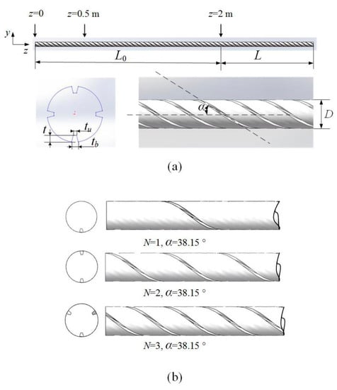
Figure 1.
(a) Geometry of PBRs and spiral ribs; (b) tubular PBRs with 1, 2 and 3 ribs and an inclined angle α = 38.15.
The diameter of tubular PBRs for large-scale outdoor cultivation is generally 50 mm [21,42,43]. Therefore, the diameter of the PBR with spiral ribs is taken as 50 mm in this work. In addition, the cross-sectional shape of the spiral ribs remains unchanged during the following calculation (t = 6 mm, tu = 3 mm, tb = 6 mm).
As shown in Figure 1a, an additional auxiliary entrance segment with spiral ribs, L0, is added to the tube for the full development of the flow and the uniformity of particle tracking (see Appendix C for a detailed discussion of the particle tracking uniformity). The length of L0 is 2 m. If backflow is found at the outlet of the PBR during the simulation, an additional 0.5 m extension section is added (not shown in Figure 1a). This addition means that the total length of the simulated model is 3 m or 3.5 m, although the length of the PBR for evaluating the L/D cycle performance and energy consumption (i.e., the L segment) is 1 m.
2.3.2. Model Meshing
The meshing of a tubular PBR with D = 50 mm, α = 38.15°, and N = 4 is shown in Figure 2. Since particle tracking has a high requirement for wall meshing and the enhanced wall function was used in the numerical calculation, the meshes were locally refined at the wall surface. The height of the first mesh layer was used to verify whether the meshing satisfied the turbulence model calculation requirements. The SST k-ω turbulence model requires the value of y+ to be approximately 1 [44], where y+ is the Reynolds number in a large eddy simulation (LES) using the wall distance y as the length dimension.
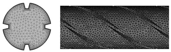
Figure 2.
Meshing of the tubular PBR (D = 50 mm, α = 38.15°, N = 4).
After repeated calculations, it is determined that at 0.5 m s−1, the height of the first layer of the boundary layer is 0.05 mm, and the boundary layer mesh contains 15 layers. The independence of the mesh was verified by examination of the pressure difference between the inlet and outlet. The result of the coarse mesh with 1.63 million cells is 1.42% different from that of the medium mesh with 4.92 million cells, and the result of the medium mesh is 2.68% different from that of fine mesh with 9.18 million cells. Thus, the medium mesh can meet the mesh independence requirements. The change in y+ for the medium mesh was obtained and is shown in Figure 3. The results show that in the vicinity of the model wall surface, the value of y+ is near 1 (the red line in Figure 3 shows y+ = 1) except for the inlet section, indicating that the mesh height of the first layer of the boundary layer is reasonable. The same meshing method was used in the other simulations in this study.
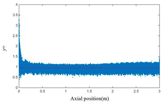
Figure 3.
Wall y+ for the medium mesh.
3. Results and discussion
3.1. Light Field and L/D Boundary
When the single-sided light is incident to the PBR along the +x-axis (Figure 4), the light path , where (x, y) are the coordinates of a point in the tube, and r is the reactor radius (m). It is assumed that the incident light intensity I0 = 800 μmol m−2 s−1 [45]. The light field on the cross section of the reactor can be obtained according to the light model shown in Section 2.3 (Figure 4b). The white line in the figure represents the L/D boundary, which is the position where Ic = 96.84 μmol m−2 s−1.
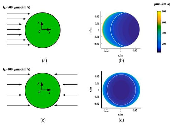
Figure 4.
Schematic diagram of illumination. (a) Single-sided illumination; (b) light field on the PBR cross section under single-sided illumination; (c) double-sided illumination; (d) light field on the PBR cross section under double-sided illumination.
When the double-sided light is incident (Figure 4c), the light intensity at a certain point on the cross section cannot be calculated using the light path of only one side. However, because the light intensity is a scalar, the light intensity at a point equals the algebraic sum of the light intensities at this point when the individual light on each side is incident separately. Since the cross-sectional area of the spiral ribs does not exceed 2.8% of the total cross-sectional area, the influence of the spiral rib interface on the light field can be ignored. The total light intensity of the double-sided illumination is assumed to be the same as that of the single-sided illumination. Hence, the intensity of the incident light on each side is I0 = 400 μmol m−2 s−1. The light field on the cross section of the reactor can be obtained according to the light model presented in Section 2.3 (Figure 4d). The white line represents the L/D boundary. Compared with the L/D boundary under the single-sided illumination conditions (Figure 4b), the L/D boundary under the double-sided illumination conditions moves toward the tube wall, and the curvature of the L/D boundary decreases, but the length of the L/D boundary increases.
3.2. Optimization of a PBR with Spiral Ribs under Single-Sided Illumination
The structural parameters of the spiral ribs and the flow rate of the algal suspension are the main factors affecting the L/D cycle performance of the algae cells. The main structural parameters of the spiral ribs include the number of spiral ribs (N), the inclination angle of the spiral ribs (α (°)), and the pitch of the spiral ribs (P (mm)). However, P and α are not independent of each other because of the linear geometric relationship between them. For example, a reactor with P = 200 mm has a spiral rib inclination angle α = 38.15°; a reactor with α = 60° has a spiral rib pitch P = 90.69 mm. Therefore, in this study, N, α, and uin were selected as influencing factors to obtain the best structural and operating parameters for the optimization of the spiral rib PBR.
The orthogonal design method was adopted to reduce the computational load and save calculation time. The factor-level table is shown in Table 1. In this study, five levels of 1, 2, 3, 4, and 5 are set for N (i.e., factor A), four levels of 15°, 30°, 45°, and 60° are set for α (i.e., factor B), and three levels of 0.4, 0.5, and 0.6 m s−1 are set for uin (i.e., factor C). Compared to the full test, which requires a total of 5 × 4 × 3 = 60 tests, the orthogonal design only requires 25 tests. The combination of factors is shown in Table 2, where the subscript represents the level of factor A, B or C. For instance, A1B4C2 represents that N is in level 1, α is in level 4, and uin is in level 2, i.e., N = 1, α = 60° and uin = 0.5 m s−1. The simulation analysis was carried out on the 25 test groups in Table 2. The average L/D cycle frequency (fav) and the efficiency of the L/D cycle enhancement (η) for each group were obtained. The data were evaluated using data analysis software, and the results are shown in Table 3.

Table 1.
Factor-level table for the orthogonal optimization of the tubular PBR.
Table 2.
Orthogonal table for optimization of the tubular PBR.
Table 3.
Significance tests for the tubular PBR with spiral ribs.
When performing the analysis of variance (ANOVA) on fav and η, the validity of the experimental data was first determined using the significance test. When the significance level is less than 0.05, the difference between the data sets can be considered statistically significant; i.e., the factor has a significant effect on the dependent variable. According to Table 3, the significance levels of N, α, and uin for both performance indicators (fav and η) are all less than 0.05, which indicates that the effects of the three factors on the two performance indicators are significant.
F refers to the F-test, which is the overall significance test. When the significance level is less than 0.05, the influence of the factor on the performance indicator can be directly evaluated by the value of F. The larger F is, the more pronounced the influence is. The F values for fav are shown in Table 3. It is obvious that F(α) >> F(N) ≅ (uin), it means that α has much greater influence on fav compared to N and uin. Similarly, the influences of the three factors on η follow the order F(N) > F(α) > F(uin).
To visualize the relationships between the three factors and the two performance indicators, the average value of fav and η at each test level was calculated and plotted in Figure 5 and Figure 6, respectively.
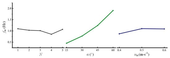
Figure 5.
Relationships between the average L/D cycle frequency and three factors (single-sided illumination).
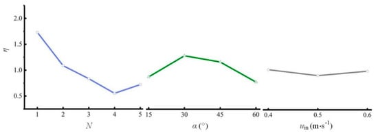
Figure 6.
Relationships between the efficiency of the L/D cycle enhancement and three factors (single-sided illumination).
Figure 5 shows that as N increases, fav first decreases and then increases. The mean of fav is the lowest with 4 spiral ribs. Increasing α can significantly increase fav. In addition, fav reaches its maximum when uin is 0.5 m s−1. The trends of the three plots show that α has the greatest influence on fav, which is consistent with the results determined based on the significance levels and the F values. Among the three plots, the optimal levels of the three factors (i.e., N = 1, α = 60°, and uin = 0.5 m s−1) correspond to the maximum values of fav. The combination of the optimal levels is group 1 in Table 2. With this combination, fav is 2.28 Hz, which is the highest of all 25 tests.
Figure 6 shows the relationships between η and the three factors. When using η as a performance indicator, the optimal N is 1, the optimal α is 30°, and the optimal uin is 0.4 m s−1. An analysis of the trends of the three plots shows that N has the greatest influence on η, while uin has the smallest influence on η. This outcome is consistent with the results determined based on the significance levels and the F values. The optimal combination of parameters corresponds to group 24 in Table 2. With this combination, η is 2.01, which is the highest of all 25 tests.
The concentration of microalgae is directly related to fav. Studies have shown that the higher fav is (below 100 Hz), the better the growth of microalgae is [16]. Of the two optimal combinations shown above, group 1 has fav of 2.28 Hz and η of 1.22, whereas group 24 has fav of 0.75 Hz and η of 2.01. fav of group 1 is much higher than that of group 24. Moreover, η of group 1 is greater than 1, which indicates that the increase in the energy consumption of group 1 is less than the increase in fav. This outcome is desirable from an economic point of view because the benefit obtained is greater than the cost. Therefore, the optimal parameter combination for the spiral rib tubular PBR under single-sided illumination is the combination in group 1, which has the following parameters: N = 1, α = 60°, and uin = 0.5 m s−1.
3.3. Optimization of the PBR with Spiral Ribs under Double-Sided Illumination
The orthogonal experiment was carried out on the tubular PBR under double-sided illumination. The influencing factors and their levels are the same as those used in the single-sided case, and the orthogonal table is the same as Table 2. The test results are shown in Table 4. Based on the significance levels and the F values, all three factors have significant effects on the L/D cycle performance under double-sided illumination. For fav, the influences of the three factors follow the order F(α) >> F(N) ≅ F(uin). For η, the influences of the three factors follows the order F(α) > F(uin) > F(N).
Table 4.
Significance test of the tubular PBR with spiral ribs (double-sided illumination).
The relationships between the three factors and the two performance indicators (fav and η) are shown in Figure 7 and Figure 8, respectively.
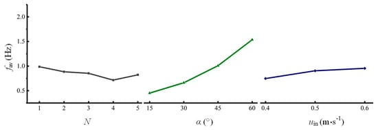
Figure 7.
Relationships between the average L/D cycle frequency and three factors (double-sided illumination).
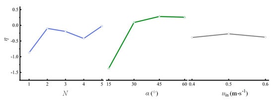
Figure 8.
Relationships between the efficiency of the L/D cycle enhancement and three factors (double-sided illumination).
Figure 7 shows that as N increases, fav first decreases and then increases. The mean of fav is the lowest with 4 spiral ribs. Increasing α can significantly increase fav. In addition, fav reaches the maximum when uin is 0.6 m/s. The trends of the three plots show that compared to N and uin, α has much greater influence on fav. This outcome is consistent with the results determined based on the significance levels and the F values.
Based on the trends of the three plots, the optimal combination of the three factors is N = 1, α = 60°, and uin = 0.6 m s−1. However, this combination is not included in the 25 combinations in Table 2. Therefore, it is necessary to remodel and recalculate the results. fav of this combination is calculated to be 2.36 Hz, which is higher than those of the 25 test groups. η of this combination is 0.60.
The relationships between η and the three factors (Figure 8) show that when η is used as the performance indicator, the optimal N is 5, the optimal α is 45°, and the optimum uin is 0.5 m s−1. This combination is group 21 in Table 2, and the corresponding η is 0.142. However, further verification shows that η of group 21 is not the highest of the 25 test groups. The efficiency of group 11 is the highest (0.53) of all 25 test groups but is still less than that of the combination of N = 1, α = 60°, and uin = 0.6 m s−1 (0.60). This outcome may occur because of the interactions between various factors, indicating that in the case of double-sided illumination, the effects of the three influencing factors are non-independent and need to be more comprehensively understood. This indication should be studied further in the future. In summary, in the case of double-sided illumination, the optimal parameter combination is N = 1, α = 60°, and uin = 0.6 m s−1.
It is worth noting that the efficiencies of the L/D cycle enhancement are negative in all cases except for three rib inclination angles (Figure 8). Based on the formula for η (Equation (17)), there are two possible reasons for these negative values: one is fav < fav,0, and the other is . A comparison of fav between the spiral rib PBRs and the plain PBR shows that the first reason (fav < fav,0) causes the negative efficiency. Under double-sided illumination, fav of the spiral rib PBR is less than that of a plain PBR under the same conditions. This result shows that the higher pumping cost does not lead to an increase in fav. Therefore, the negative efficiency of the L/D cycle enhancement is not desirable for optimizing the L/D cycle performance of the algae.
3.4. Comparison between Single-Sided and Double-Sided Illuminations and Analysis of Causes
The light field (Figure 4) shows that the L/D boundary under single-sided illumination is located only on one side of the flow field (Figure 4b), while the L/D boundary under double-sided illumination is longer and has a circular form (Figure 4d). Intuitively, a long L/D boundary can increase the probability and the number of particles participating in the L/D cycles. As a result, fav of particles under double-sided illumination should be greater than that under single-sided illumination. However, the results of the orthogonal test show that the average L/D cycle frequencies under single-sided illumination with I0 = 800 μmol m−2 s−1 are generally higher than those under double-sided illumination with I0 = 400 μmol m−2 s−1. Therefore, for a tubular PBR with spiral ribs, the use of double-sided illumination does not increase fav. In addition, under double-sided illumination, the efficiencies of the L/D cycle enhancement in the 25 tests are all less than 1 and are sometimes less than 0, which means that the increase in the pumping cost per unit time caused by the spiral ribs is greater than the increase in the L/D cycle frequency caused by the ribs. In other words, a higher pumping cost does not result in an increase in the L/D cycle frequency. The reason why double-sided illumination does not increase fav of microalgae particles can be discussed from the following three perspectives: the number of particles participating in the L/D cycles, the probability distribution of the L/D cycle frequency of the particles, and the relative position between the vortex and the L/D boundary in the reactor.
A comparison of the orthogonal test results under single-sided and double-sided illumination conditions shows that the differences in fav are large in tests 2, 5, 7, 13, 14, and 22. The corresponding average L/D cycle frequencies and the numbers of particles participating in the L/D cycles are shown in Table 5. In these six tests (including single-sided illumination and double-sided illumination), between 60% and 69.5% of the 1200 particles released are involved in the L/D cycles. The other particles do not participate in the L/D cycles; they are either always in the light zone or always in the dark zone but do not cross the L/D boundary during the time they are being tracked. The results show that fav of the particles under double-sided illumination is 15.1–24.0% lower than that under single-sided illumination. The total number of particles participating in the L/D cycles under double-sided illumination is reduced by 15.1–33.2% compared with that under single-sided illumination. Therefore, one of the reasons for the low average L/D cycle frequency under double-sided illumination is that fewer particles participate in the L/D cycle.
Table 5.
Average L/D cycle frequencies and numbers of particles participating in the L/D cycles for typical combinations under different illumination modes.
The probability density is plotted against fav under different illumination conditions for tests 2, 5, 7, 13, 14, and 22 (Figure 9). In each of these tests, the average L/D cycle frequencies of some particles increase significantly under double-sided illumination compared with that under single-sided illumination. For example, in tests 2, 5, 7, 13, and 22, the average L/D cycle frequencies of some particles can reach 6–7 Hz under double-sided illumination. However, such particles only account for a small proportion of the probability density.
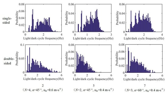
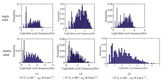
Figure 9.
Probability densities of the L/D cycle frequency for tests 2, 5, 7, 13, 14, and 22.
Taking test 22 as an example, fav of the particles under single-sided illumination ranges from 0 to 4 Hz. The range of the average L/D cycle frequencies is greater under double-sided illumination, which is 0–6.5 Hz. However, the probability density of the frequencies in the range of 4–6.5 Hz is very low. Under single-sided illumination, 47% of the 1200 released particles experience L/D cycles with frequencies of 2–4 Hz. Under double-sided illumination, this percentage is only 25%. This result shows that under double-sided illumination, the percentage of particles participating in high-frequency L/D cycles decreases. This outcome is another reason that fav of the particles under double-sided illumination is generally low.
The discussion presented above shows that fav of the particles is closely related to two factors: the number of particles participating in the L/D cycles and the probability distribution of the L/D cycle frequency of the particles. The relative position between the vortex and the L/D boundary in the reactor is the root cause of these two factors. fav is analyzed in the following section from the perspectives of the flow field and the L/D boundary.
The pressure distributions, streamlines, and L/D boundaries on the cross section in the center of the L segment (i.e., the cross section at z = 2.5 m) under different illumination modes for tests 2, 5, 7, 13, 14, and 22 are shown in Figure 10 and Figure 11. The flow field can be roughly divided into three concentric regions: the inner region (0 < r0 < 0.008 m), the middle region (0.008 < r0 < 0.016 m), and the outer region (0.016 < r0 < 0.025 m). The boundaries between the three regions are shown in red. The white dotted line in Figure 10 is the L/D boundary in the case of single-sided illumination, and the blue dotted line in Figure 11 is the L/D boundary in the case of double-sided illumination. The centers of the large vortices in these six tests are generally located in the inner region. In the case of single-sided illumination, the L/D boundaries pass through both the middle region and the outer region; in the case of double-sided illumination, the L/D boundaries are in the outer region and are annular.
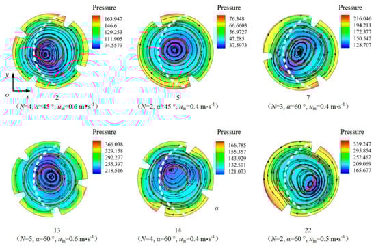
Figure 10.
Pressure distributions and L/D boundaries (single-sided illumination) on the z = 2.5 m cross section of the PBR in tests 2, 5, 7, 13, 14, and 22.
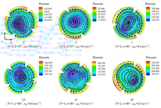
Figure 11.
Pressure distributions and L/D boundaries (double-sided illumination) on the z = 2.5 m cross section of the PBR in tests 2, 5, 7, 13, 14, and 22.
The radial position of the particle affects its L/D cycle performance. The changes in radial position of the particles initially in the inner, middle and outer regions at the inlet section of the L segment (i.e., the cross section at z = 2 m) in the six tests was studied. The results show that the movements of particles initially in the inner region are radially concentrated in the inner and middle regions, the movements of particles initially in the middle region spread across the inner, middle and outer regions, and the movements of particles initially in the outer region are radially concentrated in the outer and middle regions. Figure 12 shows the changes in the radial positions of the particles in test 2 and test 5. The L/D cycle performances of the particles in three different initial regions in the six tests were statistically studied in combination with the L/D boundary. Under single-sided illumination, 11.2–16.3% of the 1200 released particles initially in the inner region participated in the L/D cycles, 28.3–31.1% of the particles initially in the middle region participated in the L/D cycles, and 20.7–28.1% of the particles initially in the outer region participated in the L/D cycles. Similarly, under double-sided illumination, the three percentages are 7.0–10.9%, 18.1–24.6%, and 15.6%–26.5%, respectively. When single-sided illumination is switched to double-sided illumination, the numbers of particles undergoing L/D cycles are all significantly reduced regardless of their initial positions. These results show that splitting single-sided illumination into two illuminations on both sides cannot increase the number of particles undergoing the L/D cycles when using the reactor structure employed in this study.
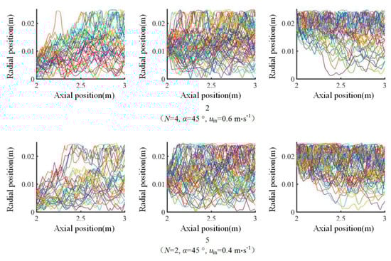
Figure 12.
Changes in the radial positions of particles in the three initial regions in test 2 and test 5.
fav of the particles in the six tests was statistically studied based on the initial positions of the particles. The statistical results are shown in Table 6. Under double-sided illumination, the average L/D cycle frequencies of the particles are all lower regardless of their initial positions. Combined with the influence of the L/D boundary on the number of particles participating in the L/D cycles, the results show that the reason for the decrease in fav is that the change in the position of the L/D boundary not only reduces the number of particles undergoing the L/D cycles but also decreases the L/D cycle frequencies of the particles in the different regions.
Table 6.
Average L/D cycle frequencies of particles in three regions under single-sided and double-sided illuminations for tests 2, 5, 7, 13, 14, and 22 (arrows represent the relative changes in frequency; ↑ is increased, ↓ is decreased).
3.5. Development and Validation of a Method for Increasing the Average L/D Cycle Frequency
The flow field determines the radial position of the particles, and the light field determines the position of the L/D boundary. The phenomenon in which particles participate in the L/D cycles is a result of the synergy between the flow field and the light field. Therefore, two methods could be considered to increase the number of particles participating in the L/D cycles and the percentage of particles participating in the high-frequency L/D cycles, thereby increasing fav of the particles: changing the flow field (the vorticity field) by changing the structure of the reactor so that more particles can pass through the L/D boundary and changing the position of the L/D boundary based on the radial position of the particles in the flow field. The second method is validated below.
It was shown in Section 3.4 that the movements of particles initially in the inner region are radially concentrated in the inner and middle regions, and the movements of particles initially in the outer region are radially concentrated in the middle and outer regions. The L/D boundaries discussed above under different illumination modes do not pass through the inner regions, as shown in Figure 10 and Figure 11. Therefore, it is assumed that the L/D boundary can pass through the three regions simultaneously by adjusting the light intensity and the incident direction, as shown in Figure 13, where the white line is the L/D boundary.
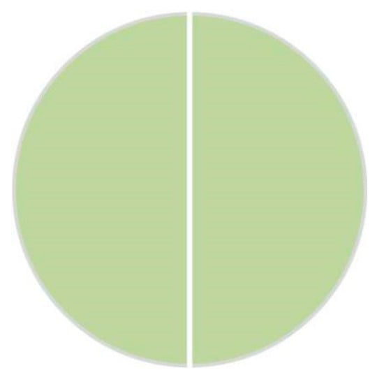
Figure 13.
Schematic diagram of the L/D boundary.
fav under the conditions shown in Figure 13 was calculated for the 25 test groups in the orthogonal test. The result is compared with that obtained under single-sided illumination conditions (Figure 14). Adjusting the position and curvature of the L/D boundary according to the flow field increases fav of the particles. This increase occurs because the change in the L/D boundary increases the number of particles undergoing the L/D cycles, and the change in the L/D boundary can simultaneously increase the percentage of particles involved in the high-frequency L/D cycles. Taking group 6, which has the largest frequency increase, as an example, the number of particles participating in the L/D cycles under the conditions shown in Figure 13 is 59.1% higher than that under the single-sided illumination conditions. The probability density function (Figure 15) shows that the L/D cycle frequencies of most of the particles is near 1 Hz under the conditions shown in Figure 13. The percentage of particles participating in the high-frequency L/D cycles under these conditions is significantly higher than that under single-sided illumination. The increase in fav of the optimal combination under single-sided illumination (group 1 in Table 2) is the smallest (only 26.3%). These results show that in the case of single-sided illumination, the synergy between the flow field and the light field of group 1 is good.
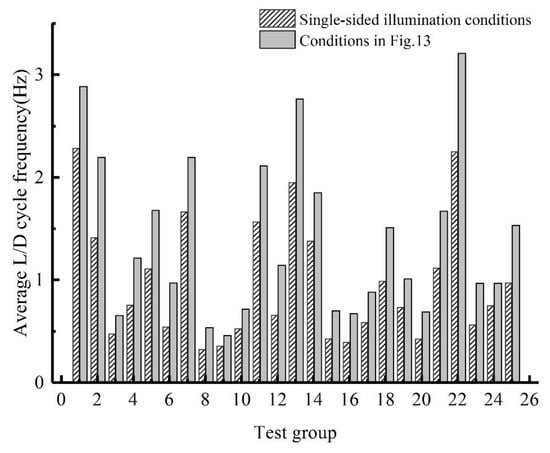
Figure 14.
Average L/D cycle frequency for each orthogonal test group under single-sided illumination conditions and under the conditions shown in Figure 13.
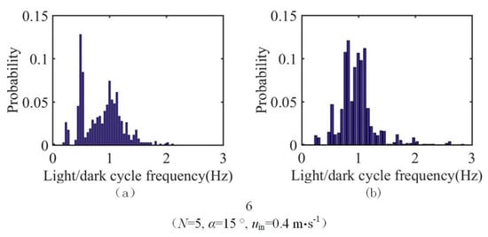
Figure 15.
Probability densities of the L/D cycle frequency for group 6 under (a) single-sided illumination conditions; and (b) conditions shown in Figure 13.
4. Conclusions
In this study, the orthogonal design method was used to optimize the structural and operating parameters of a tubular PBR with spiral ribs. The average L/D cycle frequency (fav) and the efficiency of the L/D cycle enhancement (η) were selected as performance indicators. The results show that switching the single-sided parallel light illumination with a light intensity of I0 = 800 μmol m−2 s−1 to double-sided illumination with half of the light intensity on each side does not increase fav. Double-sided illumination also reduces η, which indicates that a higher energy input does not result in corresponding benefits. The orthogonal test shows that under single-sided illumination, the spiral rib inclination angle (α) has much greater influence on fav compared to the number of spiral ribs (N) and the inlet velocity of the algal suspension (uin). Moreover, N has the greatest influence on η, α has the next greatest influence, and uin has the smallest influence. Under single-sided illumination, the optimal parameter combination is N = 1, α = 60°, and uin = 0.5 m s−1. With this combination, fav of the spiral rib PBR reaches 2.28 Hz, which is 4.3 times higher than that of a plain PBR under the same conditions, and η is 1.22. The synergy between the flow field and the light field affects the number of particles participating in the L/D cycles and the probability density distribution of the L/D cycle frequency of these particles, thereby affecting fav and η. To promote the synergy between the flow field and the light field, we can adjust the relative position between the L/D boundary and the vortex in the flow field by changing the vorticity field or by changing the light field so the L/D boundary passes through the center of the vortex. In this case, fav is remarkably improved compared with the case where the L/D boundary line passes through the edge region of the vortex.
Author Contributions
Y.L., J.W. (Jing Wang), and J.W. (Jing Wu) conceived and structured the study. Y.L., and J.W. (Jing Wang) developed the model and analyzed the results. Y.L. prepared the preliminary manuscript. J.W. (Jing Wu) revised and finalized the manuscript and obtained funding for the project.
Funding
This research was funded by the National Natural Science Foundation of China, grant number 51576075.
Conflicts of Interest
The authors declare no conflict of interest.
Appendix A
If the number of tracked particles is not enough, the final result is significantly affected by randomness and lacks reliability. Therefore, the number of tracked particles needs to be determined.
The number of tracked particles was validated on a reactor with a number of ribs N = 2, 4, 6, and 8 and an inclination angle α = 38.15°. The validation result is shown in Figure A1. When the number of particles is less than 400, the average L/D cycle frequency increases significantly with the number of particles; when the number of particles is greater than 400, the average L/D cycle frequency does not change significantly with the number of particles. In this study, the number of released particles is chosen to be 1200 to eliminate the random effects caused by too few particles on the results.

Figure A1.
Average L/D cycle frequency of particles as a function of the particle number for PBRs with different numbers of ribs.
Appendix B
After the particles are released, it takes a certain amount of time for the particles to completely pass through the entire photobioreactor (PBR). If the particle tracking time is too short, the particles do not complete their movement across the reactor, and the result is unreliable; if the particle tracking time is too long, computing resources are wasted. Therefore, it is necessary to determine the appropriate particle tracking time.
The particle tracking time was validated on a reactor with a number of ribs N = 2, 4, 6, and 8 and an inclination angle α = 38.15°. The validation result is shown in Figure A2. When the tracking time is less than 30 s, the average L/D cycle frequency of the microalgal particles changes significantly with time; when the tracking time is more than 30 s, the average L/D cycle frequency does not change much with time. The particle tracking time is set to 120 s in this study to ensure the complete movement of particles in the tubular PBR.

Figure A2.
Average L/D cycle frequency of particles as a function of particle tracking time for PBRs with different numbers of ribs.
Appendix C
In actual culture under well-mixed conditions, the algal cells are evenly distributed in the liquid medium, and the algal liquid can be considered approximately uniform. In the case of particle tracking, each particle represents a single algal cell. Therefore, the particles should also be approximately evenly distributed in the simulated space under well-mixed conditions. The group release method was adopted in this study to save computing resources. In this method, the particles are simultaneously released from a circular domain on a cross section. When the particle group is released, it is necessary to add an auxiliary segment before the L segment (i.e., to release the particles before the entrance to the L segment). This auxiliary segment ensures that the particles can be approximately evenly distributed on the cross section at the entrance of the L segment. The length that is needed for the auxiliary segment is investigated below.
First, the particles were released on a circular domain of a cross section. Then, the distributions of the particles on different cross sections along the axial direction were observed to determine whether the particles were evenly distributed on the cross section. Figure A3 shows the movement of the particles. Figure A3a shows that after moving 0.5 m, the particles are mainly concentrated in the center of the cross section rather than being evenly distributed over the entire cross section. It was found that after moving 1.5 m, the particles are no longer concentrated in the center of the cross section and can be considered as being approximately evenly distributed (Figure A3b). Figure A3c shows the change in the radial positions of the particles. Based on Figure A3c, a certain movement time and axial distance are required for the particles to be evenly distributed over different radial positions. According to the cross-sectional particle distributions, a movement distance of 1.5 m can ensure that the particles are evenly distributed on each cross section. Therefore, the particles are released at z = 0.5 m, as shown in Figure 1a.

Figure A3.
Schematic diagram of particle movement. (a) Cross-sectional distribution of particles after 0.5 m movement; (b) Cross-sectional distribution of particles after 1.5 m movement; (c) Radial positions of particles along the axial direction.
References
- Huesemann, M.H.; Benemann, J.R. Biofuels from microalgae: Review of products, processes and potential, with special focus on dunaliella sp. In The Alga Dunaliella Biodiversity, Physiology, Genomics and Biotechnology; Ben-Amotz, A., Polle, J.E.W., Subba Rao, D.V., Eds.; CRC Press: Boca Raton, FL, USA, 2009. [Google Scholar]
- Raut, N.; Al-Balushi, T.; Panwar, S.; Vaidya, R.S.; Shinde, G.B. Microalgal biofuel. In Biofuels-Status and Perspective; Biermat, K., Ed.; Intech: Rijeka, Croatia, 2015; Volume 6, pp. 101–140. [Google Scholar]
- Klassen, V.; Blifernez-Klassen, O.; Wobbe, L.; Schlüter, A.; Kruse, O.; Mussgnug, J.H. Efficiency and biotechnological aspects of biogas production from microalgal substrates. J. Biotechnol. 2016, 234, 7–26. [Google Scholar] [CrossRef] [PubMed]
- Klassen, V.; Blifernez-Klassen, O.; Wibberg, D.; Winkler, A.; Kalinowski, J.; Posten, C.; Kruse, O. Highly efficient methane generation from untreated microalgae biomass. Biotechnol. Biofuels 2017, 10, 186. [Google Scholar] [CrossRef] [PubMed]
- Razzak, S.A.; Hossain, M.M.; Lucky, R.A.; Bassi, A.S.; DeLasa, H. Integrated CO2, capture, wastewater treatment and biofuel production by microalgae culturing—A review. Renew. Sust. Energy Rev. 2013, 27, 622–653. [Google Scholar] [CrossRef]
- Grossman, A.R. Chlamydomonas reinhardtii and photosynthesis: Genetics to genomics. Curr. Opin. Plant Biol. 2000, 2, 132–137. [Google Scholar] [CrossRef]
- Qin, S.; Lin, H.; Jiang, P. Advances in genetic engineering of marine algae. Biotechnol. Adv. 2012, 30, 1602–1613. [Google Scholar] [CrossRef] [PubMed]
- Yang, B.; Liu, J.; Liu, B.; Sun, P.; Ma, X.; Jiang, Y.; Wei, D.; Chen, F. Development of a stable genetic system for chlorella vulgaris —a promising green alga for CO2 biomitigation. Algal Res. 2015, 23, 134–141. [Google Scholar] [CrossRef]
- Run, C.; Fang, L.; Fan, C.; Luo, Y.; Hu, Z.; Li, Y. Stable nuclear transformation of the industrial alga chlorella pyrenoidosa. Algal Res. 2016, 17, 196–201. [Google Scholar] [CrossRef]
- Borowitzka, M.A.; Moheimani, N.R. Algae for Biofuels and Energy; Springer: Berlin/Heidelberg, Germany, 2013; pp. 133–152. [Google Scholar]
- Wang, B.; Li, Y.; Wu, N.; Lan, C.Q. CO2 bio-mitigation using microalgae. Appl. Microbiol. Biotechnol. 2008, 79, 707–718. [Google Scholar] [CrossRef] [PubMed]
- Wongluang, P.; Chisti, Y.; Srinophakun, T. Optimal hydrodynamic design of tubular photobioreactors. J. Chem. Technol. Biotechnol. 2013, 88, 7. [Google Scholar] [CrossRef]
- Laws, E.A.; Terry, K.L.; Wickman, J.; Chalup, M.S. A simple algal production system designed to utilize the flashing light effect. Biotechnol. Bioeng. 1983, 25, 2319–2335. [Google Scholar] [CrossRef]
- Vejrazka, C.; Marcel, J. Photosynthetic efficiency and oxygen evolution ofchlamydomonas reinhardtiiunder continuous and flashing light. Appl. Microbiol. Biotechnol. 2013, 97, 1523–1532. [Google Scholar] [CrossRef] [PubMed]
- Huang, J.; Li, Y.; Wan, M.; Yan, Y.; Wang, W. Novel flat-plate photobioreactors for microalgae cultivation with special mixers to promote mixing along the light gradient. Bioresour. Technol. 2014, 159, 8–16. [Google Scholar] [CrossRef] [PubMed]
- Liao, Q.; Li, L.; Chen, R.; Zhu, X. A novel photobioreactor generating the light/dark cycle to improve microalgae cultivation. Bioresour. Technol. 2014, 161, 186–191. [Google Scholar] [CrossRef] [PubMed]
- Zhang, Q.; Xue, S.; Yan, C.; Wu, X.; Wen, S.; Cong, W. Installation of flow deflectors and wing baffles to reduce dead zone and enhance flashing light effect in an open raceway pond. Bioresour. Technol. 2015, 198, 150–156. [Google Scholar] [CrossRef] [PubMed]
- Yoshimoto, N.; Sato, T.; Kondo, Y. Dynamic discrete model of flashing light effect in photosynthesis of microalgae. J. Appl. Phycol. 2005, 17, 207–214. [Google Scholar] [CrossRef]
- Hu, J.Y.; Sato, T. A photobioreactor for microalgae cultivation with internal illumination considering flashing light effect and optimized light-source arrangement. Energy Convers. Manag. 2017, 133, 558–565. [Google Scholar] [CrossRef]
- Perner-Nochta, I.; Posten, C. Simulations of light intensity variation in photobioreactors. J. Biotechnol. 2007, 131, 276–285. [Google Scholar] [CrossRef]
- Gómez-Pérez, C.A.; Espinosa, J.; Ruiz, L.C.M.; van Boxtel, A.J.B. CFD simulation for reduced energy costs in tubular photobioreactors using wall turbulence promoters. Algal Res. 2015, 12, 1–9. [Google Scholar] [CrossRef]
- Qin, C.; Lei, Y.; Wu, J. Light/dark cycle enhancement and energy consumption of tubular microalgal photobioreactors with discrete double inclined ribs. Bioresour. Bioprocess 2018, 5, 28. [Google Scholar] [CrossRef]
- Zhang, Q.; Wu, X.; Xue, S.; Liang, K.; Cong, W. Study of hydrodynamic characteristics in tubular photobioreactors. Bioprocess Biosyst. Eng. 2013, 36, 143–150. [Google Scholar] [CrossRef]
- Qin, C.; Wu, J. Influence of successive and independent arrangement of Kenics mixer units on light/dark cycle and energy consumption in a tubular microalgae photobioreactor. Algal Res. 2019, 37, 17–29. [Google Scholar] [CrossRef]
- Qin, C.; Wu, J.; Wang, J. Synergy between flow and light fields and its applications to the design of mixers in microalgal photobioreactors. Biotechnol. Biofuels 2019, 12, 93. [Google Scholar] [CrossRef] [PubMed]
- Menter, F.R. Two-equation eddy-viscosity turbulence models for engineering applications. AIAA J. 1994, 32, 1598–1605. [Google Scholar] [CrossRef]
- Sato, T.; Usui, S.; Tsuchiya, Y.; Kondo, Y. Invention of outdoor closed type photobioreactor for microalgae. Energy Convers. Manag. 2006, 47, 791–799. [Google Scholar] [CrossRef]
- Fluent, A. Ansys Fluent Theory Guide; ANSYS Incorporated: Canonsburg, PA, USA, 2011; pp. 724–746. [Google Scholar]
- Molina, E.; Fernández, J.; Acién, F.G.; Chisti, Y. Tubular photobioreactor design for algal cultures. J. Biotechnol. 2001, 92, 113–131. [Google Scholar] [CrossRef]
- Pruvost, J.; Legrand, J.; Legentilhomme, P.; Mullerfeuga, A. Lagrangian trajectory model for turbulent swirling flow in an annular cell: Comparison with residence time distribution measurements. Chem. Eng. Sci. 2002, 57, 1205–1215. [Google Scholar] [CrossRef]
- Gómez-Pérez, C.A.; Oviedo, E.J.; Ruiz, M.L.C. Twisted tubular photobioreactor fluid dynamics evaluation for energy consumption minimization. Algal Res. 2017, 27, 65–72. [Google Scholar] [CrossRef]
- Huang, J.; Feng, F.; Wan, M.; Ying, J.; Li, Y.; Qu, X.; Pan, R.; Shen, G.; Li, W. Improving performance of flat-plate photobioreactors by installation of novel internal mixers optimized with computational fluid dynamics. Bioresour. Technol. 2015, 182, 151–159. [Google Scholar] [CrossRef]
- Pruvost, J.; Cornet, J.F.; Legrand, J. Hydrodynamics influence on light conversion in photobioreactors: An energetically consistent analysis. Chem. Eng. Sci. 2008, 63, 3679–3694. [Google Scholar] [CrossRef]
- Moberg, A.K.; Ellem, G.K.; Jameson, G.J.; Herbertson, J.G. Simulated cell trajectories in a stratified gas–liquid flow tubular photobioreactor. J. Appl. Phycol. 2012, 24, 357–363. [Google Scholar] [CrossRef]
- Schuster, A. Radiation through a foggy atmosphere. Astrophys. J. 1903, 26, 379–381. [Google Scholar] [CrossRef]
- Loubière, K.; Olivo, E.; Bougaran, G.; Jérémy, P.; Robert, R.; Legrand, J. A new photobioreactor for continuous microalgal production in hatcheries based on external-loop airlift and swirling flow. Biotechnol. Bioeng. 2009, 102, 132–147. [Google Scholar] [CrossRef] [PubMed]
- Luo, H.P.; Al-Dahhan, M.H. Analyzing and modeling of photobioreactors by combining first principles of physiology and hydrodynamics. Biotechnol. Bioeng. 2004, 85, 382–393. [Google Scholar] [CrossRef] [PubMed]
- Huang, J.; Kang, S.; Wan, M.; Li, Y.; Qu, X.; Feng, F.; Wang, J.; Wang, W.; Shen, G.; Li, W. Numerical and experimental study on the performance of flat-plate photobioreactors with different inner structures for microalgae cultivation. J. Appl. Phycol. 2015, 27, 49–58. [Google Scholar] [CrossRef]
- Acién Fernández, F.G.; Hall, D.O.; Cañizares Guerrero, E.; Krishna, R.K.; Molina, G.E. Outdoor production of phaeodactylum tricornutum biomass in a helical reactor. J. Biotechnol. 2003, 103, 137–152. [Google Scholar] [CrossRef]
- Molina, E.; Fernández, F.G.A.; Camacho, F.G.; Rubio, F.C.; Chisti, Y. Scale-up of tubular photobioreactors. J. Appl. Phycol. 2000, 12, 355–368. [Google Scholar] [CrossRef]
- Sorokin, C.; Krauss, R.W. The effects of light intensity on the growth rates of green algae. Plant Physiol. 1958, 33, 109–113. [Google Scholar] [CrossRef]
- Norsker, N.H.; Barbosa, M.J.; Vermuë, M.H.; Wijffels, R.H. Microalgal production—A close look at the economics. Biotechnol. Adv. 2011, 29, 24–27. [Google Scholar] [CrossRef]
- Slegers, P.M.; van Beveren, P.J.M.; Wijffels, R.H.; van Straten, G.; van Boxtel, A.J.B. Scenario analysis of large scale algae production in tubular photobioreactors. Appl. Energy 2013, 105, 395–406. [Google Scholar] [CrossRef]
- Versteeg, H.K.; Malalasekera, W. Introduction to Computational Fluid Dynamics, 2rd ed.; Prentice Hall: Upper Saddle River, NJ, USA, 2007. [Google Scholar]
- Perner-Nochta, I.; Lucumi, A.; Posten, C. Photoautotrophic cell and tissue culture in a tubular photobioreactor. Eng. Life Sci. 2007, 7, 127–135. [Google Scholar] [CrossRef]
© 2019 by the authors. Licensee MDPI, Basel, Switzerland. This article is an open access article distributed under the terms and conditions of the Creative Commons Attribution (CC BY) license (http://creativecommons.org/licenses/by/4.0/).