Abstract
This study of process heat source change in industrial conditions has been developed to aid engineers and energy managers with working towards sustainable production. It allows for an objective assessment from energetic, environmental, and economic points of view, thereby filling the gap in the systematic approach to this problem. This novel site-wide approach substantially broadens the traditional approach, which is based mostly on “cheaper” and “cleaner” process heat sources’ application and only takes into account local changes, while neglecting the synergic effect on the whole facility’s operations. The mathematical model employed assesses the performance change of all the affected refinery parts. The four proposed aromatic splitting process layouts, serving as a case study, indicate feasible heat and condensate conservation possibilities. Although the estimated investment needed for the most viable layout is over €4.5 million, its implementation could generate benefits of €0.5–1.5 million/year, depending on the fuel and energy prices as well as on the carbon dioxide emissions cost. Its economics is most sensitive to the steam to refinery fuel gas cost ratio, as a 10% change alters the resulting benefit by more than €0.5 million. The pollutant emissions generated in the external power production process contribute significantly to the total emissions balance.
1. Introduction
The oil and petroleum industry is among the most energy-intense industrial sectors. Energy consumption in this sector in 2012 in OECD countries represented more than 7% of the total from industry [1]. The available literature states that a 10–20% energy consumption reduction is feasible in U.S. refineries with economically acceptable parameters [2]; in Russia, the situation is similar [3]. Heat recuperation intensification [4,5], modern electromotor installations [6,7], advanced process control implementation [6,8], improvement of fuel gas management and fuel switching [5,8], and the use of new conversion technologies [8,9] are among the most promising measures to achieve the energy intensity reduction goal. An additional benefit, although less tangible than direct energy cost reduction, is an associated cut in the GHG emissions [9,10] emitted from process heaters. Analogous measures can be applied to combined heat and power plants [11,12,13], which often serve as steam suppliers for industrial facilities. The resulting benefits can be further enhanced if oxy-combustion is applied [14,15,16]. The reduction of fire and explosion risk should also be taken into account as an additional reason for such an investment.
Direct fuel consumption and associated emissions, which contribute a major part of the total energy consumption in a refinery, are attributed to process heaters and steam boilers [17,18]. Heavy fuel oils and refinery fuel gas represented the majority of fuels used in both cases [19,20]. The scheduling of a fuel gas network represents a challenge for a refinery due to both its multiple sources and its variable composition [21,22], as well as its variable production and demand [23,24]. The flexibility to switch between various types of fuel consumed seems to be an attractive economic route to deal with this challenge [25,26]. As discussed below in more detail, this flexibility may include natural gas or hydrogen-rich gases [26,27], and can be exploited on a national or a global level [28]. The associated decrease in emissions [29] and possible change in the refinery electric energy balance if fuel gas is used for cogeneration purposes [30] may represent additional drivers for fuel management improvement. Fuel and flare gas management system improvement has been introduced in various studies; producing reformatted [31,32] or recovered material [33,34] is another viable option for exploiting the material value instead of energetic refinery fuel gas content. Several studies investigated the possibility of replacing refinery fuel gas with hydrogen, thereby increasing the fuel system flexibility and decreasing the GHG emissions [35,36]. These studies show that the fuel consumption by industry may be subject to single- or multipurpose optimization, and that it can decrease its environmental impact and still be economically beneficial.
Weydahl et al. [35] explored the possibility of replacing fuel gas in a process furnace with hydrogen produced by steam methane reforming. Similarly, Lowe et al. [36] investigated the technical details of fuel gas to hydrogen combustion in fired heaters at one of Chevron’s refineries, especially regarding the change in heat flux and the required burner adjustments. They concluded that it is technically feasible, but associated with high investment costs. Higher NOx emissions are to be expected as well, due to a higher flame temperature. Lee et al. [26] proposed and tested natural gas switching to hydrogen-rich tail gas in a fired heater located in a hydrotreater unit, which resulted in flame shortening, a NOx emissions increase, and a slight thermal efficiency decrease. Fonseca et al. [19] proposed changing the fuel in the central CHP unit in a refinery located in Portugal, coupled with gas turbine installation, and claimed to have improved the energy efficiency of the CHP unit and reduced SOx and NOx emissions. Gabr et al. [27] addressed the possibility of pollutant emissions decreasing in a hydrotreater unit by switching from fuel oil to natural gas in the fired heater. This experiment provided heat integration improvement and substantial financial savings, along with emission reduction. Rehfelt et al. [6], in their bottom-up study, presented a systematic approach to suitable fuel selection in fired process heaters, including the technological details of particular processes. Fuel price, carbon dioxide emissions, and technological infrastructure are the key factors influencing the fuel choice. Cogeneration potential has not been studied, however.
The above literature survey indicates that significant attention has been paid either to process furnaces or to CHP units where fuel switching can be performed directly, e.g., fuel oil to natural gas, or fuel gas to hydrogen. Carbon dioxide emission decrease can be seen as the major driving force in fuel switching process studies. Situations where water steam acts as the heat carrier, enabling a simultaneous fuel consumption change in refinery furnaces and CHP units, require a more complex approach, which, as we learned from our literature survey, is missing from the current literature. This approach should include the impact on emissions, possible energy production changes, and the resulting project economics, following multiple optimization criteria.
The goal of our study is a complex assessment of the scope of process heat source switching, comprising all of the abovementioned factors. As documented in the relevant literature, such a broad approach to this problem and the resulting general methodology have not yet been presented.
The novelty of the developed methodology, as presented in this paper and tested via a suitable case study, is its systematic approach to fuel switching assessment. It therefore has the potential to convey relevant findings to both academics and industry. The employed mathematical model includes the material and heat balances of the process itself and its impact on the CHP unit operation, both from a fuel consumption and a cogeneration potential exploitation point of view. Seasonal CHP unit operation modes were taken into account to present an even more realistic assessment. The emissions changes, in refineries as well as outside them, caused by electricity balance changes were also included, following the guidelines set by valid EU legislation.
The aromatics fractionation process was chosen as a suitable case study as it is among the most energy-intensive processes in a conventional refinery [37] due to the close boiling points of the individual fractions and compounds. A conventional aromatics extraction and fractionation process includes fractionation columns that may be reboiled, either by water steam condensers or by furnaces fired by refinery fuel gas or fuel oil. Usually, an industrial CHP unit [38,39] is a marginal source of water steam consuming various types of fuel to produce high-pressure water steam for electricity and heat cogeneration in steam turbines. Introducing water steam as a heat carrier can, among other benefits, help to reduce the fire and explosion risk in the refinery.
In this paper, the problem’s superstructure is defined first, followed by a general mathematical model covering all relevant aspects addressed in the introduction. The selected aromatics plant is then presented in a more detailed manner, including further model equations and assumptions along with the available process data. Because of industrial data confidentiality, the raw data are not provided. Calculation and sensitivity analyses’ results are discussed, and the relevant findings summed up, in the conclusions section.
2. Materials and Methods
2.1. General Problem Superstructure and Assessment
The general refinery structure and material and the energy flows of the analyzed problem are depicted in Figure 1.
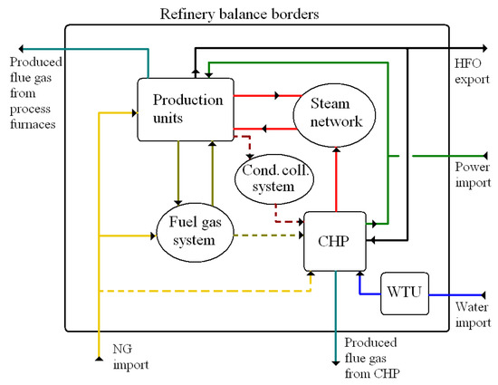
Figure 1.
Schematic depiction of refinery superstructure. CHP = combined heat and power unit; Cond. coll. = steam condensates collection; HFO = heavy fuel oil; NG = natural gas; WTU = water treatment unit.
A complex calculation including all affected systems and streams has to be considered in the case of heat source switching from fuel gas to steam because:
- The fuel gas system balance is maintained by adding natural gas. A temporary fuel gas excess can be solved by its rerouting to the CHP. A change in the fuel gas system balance results either in natural gas import decrease or in rerouting a part of the fuel gas to the CHP. These options lead to different economic and environmental assessment results.
- The CHP unit is likely to be equipped with steam boilers, coupled with backpressure and condensing steam turbines that act as a sufficiently flexible marginal steam source for the refinery. A change in steam consumption on one or several pressure levels leads to a fuel consumption change as well as a change in power production. Both effects have to be incorporated in the process model.
- CHP unit steam boilers are usually equipped with deNOx and deSOx systems. Process furnaces, on the other hand, especially older and smaller ones, likely do not use any of these.
- A condensates collection system may or may not be in operation; the latter condition is more probable in older production units. The operational efficiency affects the CHP unit thermal efficiency.
- A steam network’s operation is affected by changes in steam balance. Cold spots or spots with high steam velocity might appear; the former leads to increased heat loss from steam pipelines and the latter to undesired steam pressure drop. Measures to avoid these situations should be included in the economic assessment.
- A change in the refinery power import results in a change in emissions generation elsewhere. This fact must be incorporated in any complex environmental evaluation.
The mathematical model describing the situation characterized above consists of the following parts:
- Model of analyzed processes;
- Water steam consumption estimation in new column reboilers after process heat source switching;
- Simplified model of CHP unit;
- GHG emissions balance difference before and after process heat source change;
- Economic assessment including total capital costs estimation, economic balance, and payback period calculation.
2.1.1. General Process Model
Figure 2 depicts a general flow diagram of a furnace-fired distillation column—a system frequently employed for the separation of components with higher boiling points.
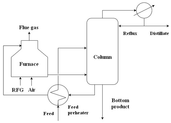
Figure 2.
General flow diagram of a furnace-fired distillation column.
For a system with j material streams and feed consisting of i components split into product streams, the following equations apply: Equation (1) defines the j-th stream density at stream temperature, Tj, Equation (2) its average isobaric heat capacity in the range between the reference temperature, Tref, and steam temperature, Tj, and Equation (3) defines its specific heat of evaporation at the temperature, Tj:
This allows for reboiler heat duty estimation (Equation (4)), provided that the volumetric flows, composition, and temperatures of individual streams are known:
In Equation (4), the meaning of the subscripts is as follows: BP = bottom product, D = distillate, ovhd = overhead vapors, R = reflux, reb = reboiler, ref = reference.
In case a feed preheater is present, the feed temperature, Tfeed, is that of the feed before the preheating. If the heat losses from the column and reboiler can be neglected, Equation (5) defines the equality of reboiler duty, , and process-side furnace duty, :
A single furnace may be used to reboil several columns via the circulating bottom product in a more integrated process layout. The furnace process side duty can then be estimated from Equation (6), where the individual reboiler duties of c columns are estimated using Equations (1) to (4). Alternatively, process heat duties can be estimated from the circulating bottom product heat balance (Equation (7)) if the circulating stream mass flow, , and temperatures at the reboiler inlet, , and outlet, , are known:
The furnace-side furnace duty of the k-th furnace is estimated by Equation (8), assuming that the fuel mass flow and composition are known and sufficient measured process data exist to calculate the mass and heat balance of its combustion. Thereby, the enthalpy flows associated with the combustion inlet air, , and with the released flue gas, , can be calculated. Heat loss from the k-th furnace, , can best be estimated as its design heat loss obtained from furnace documentation.
The lower heating value of the fuel used in the furnaces (refinery fuel gas) can be obtained by Equation (9), assuming known fuel gas composition of i constituents.
Combustion air is frequently preheated with low-pressure steam to save fuel. The associated steam consumption results from the preheating heat balance:
The theoretical oxygen consumption for complete fuel combustion results from general fuel combustion stoichiometry:
This calculation can be verified through the good agreement of the process-side and furnace-side furnace heat duties. If any discrepancies exist between these two, the calculation procedure as well as the process data reliability should be checked.
2.1.2. Steam Consumption in New Column Reboilers and Condensates Management
Let us consider the high-pressure (typically 30 to 40 bar) steam available in a refinery as an alternative process heat source to refinery fuel gas. If it has a sufficiently high condensing temperature to serve as a process heat source instead of the k-th furnace, its consumption in a new column reboiler is calculated by Equation (12):
Summing up the calculated high-pressure steam consumption replacing the process heat from furnaces, the total change in the high-pressure steam consumption in a refinery is obtained via Equation (13):
Steam condensate can be assumed to leave the reboilers as boiling liquid at HPS pressure. Thus, its heat content is still high and its pressure is decreased in a flash vessel, usually to LPS pressure [38,39]. Low-pressure flash steam is thus produced; its mass flow is estimated via Equation (14) and its production decreases LPS import from the CHP unit, which usually serves as a marginal steam source for the refinery on all main steam pressure levels.
The remaining steam condensate is then either pumped back to the CHP unit to be reused for steam production [38,39] or disposed of if the condensates collection system is absent.
2.1.3. Combined Heat and Power Unit (CHP)
An industrial CHP unit consisting of heavy fuel-oil-fired, high-pressure steam boilers, backpressure and extraction-condensing steam turbines, and a boiler feedwater preparation system was considered. Boiler feedwater was prepared from a mixture of collected condensates from the refinery, turbine condensates, and fresh chemically treated water.
A change in steam export, , on the p-th pressure level from a CHP unit resulted in a marginal change in fuel energy consumption, . Total fuel energy consumption change, , can be calculated by Equation (15), taking into account the change in the exported steam mass flow, its specific enthalpy, , the specific enthalpy of imported water, (either the collected condensate from a refinery or cold chemically treated water, depending on the system layout) and the marginal thermal efficiency of the CHP unit, .
A change in fuel energy consumption can be directly converted to a change in its consumption, , by employing its lower heating value:
The marginal thermal efficiency of a CHP unit based on steam boilers and turbines reflects the change in heat and material (steam, water) losses caused by a change in water steam production [40]. Stack losses make a major contribution to these losses; thus, it is mostly the change in boiler thermal efficiency that contributes to the final value. It is known that a large industrial steam boiler’s thermal efficiency is almost constant at a steam production rate above 40% of the nominal one. It can thus be concluded that there is no significant difference between the nominal and marginal boiler thermal efficiency during standard boiler operation. The same goes for the whole CHP unit based on steam boilers and turbines. The nominal CHP unit thermal efficiency can be found in the literature, e.g., [41].
A change in the energy production of a CHP plant, associated with changed steam export , can be expressed by Equation (17), where α represents the portion of electric energy consumed internally (driving CHP unit boiler fans, feedwater pumps etc.) due to steam export change:
The value of 0.05 can be adopted for α without a substantial loss of accuracy for CHP units based on steam boilers and steam turbines [41]; represents the marginal electric energy production change, associated with the steam export change on the p-th pressure level. Its values for individual exported steam pressure levels can be derived from the steam turbine models developed by Mavromatis and Kokossis [42] and Varbanov et al. [43] as the value of specific enthalpy difference between the turbine inlet and the outlet steam at the p-th pressure level during isoentropic (ideal) expansion. The specific enthalpic difference of inlet and outlet steam in a steam turbine can either be calculated using the developed models [44,45] or estimated using the enthalpy–entropy diagram for water steam, as employed by Mrzljak et al. [46].
The CHP unit imports fresh, chemically treated water from the water treatment plant. The water import change, , can be estimated by Equation (18) considering the total steam export change, , the condensates returned to the CHP unit, , and water losses in the CHP unit (water and steam leaks and vents, boiler blowdown), assuming a water excess coefficient of φ = 0.05 [41].
2.1.4. Emissions from Combustion Processes
The issue of industrial emissions control is dealt with by European legislation (Directive 2010/75/EU [47]), which has been followed by national regulations in the member states. In order to correctly compare the emissions from various combustion processes, the legislation (Directive 2010/75/EU, Annex V [47]) defines the reference conditions to which the emissions are related:
- complete fuel combustion;
- dry flue gas;
- normal state conditions (101.3 kPa and 0 °C);
- the oxygen amount in the flue gas is set to a reference value for various fuels.
Large emission producers are obliged to publicly report their emissions released to the atmosphere. Once a characteristic (or average) r-th fuel composition is known, the combustion mass balance, based on Equation (11) and the above conditions, can be found, yielding specific normal dry flue gas volume released per 1 kg (or 1 L or 1 normal cubic meter) of r-th fuel combusted . Multiplying this figure by the reported individual n-th pollutant emission level from the r-th fuel combustion process, , the specific pollutant emissions, , can be obtained:
Specific pollutant emissions from electricity production, [g/MWh], can be estimated in a similar way, once an appropriate energy mix for the electric energy production is selected. Changes in the n-th pollutant production in the refinery and the overall n-th pollutant production can be expressed as follows:
Emission costs are related to pollutant production change and their specific cost, cn. For carbon dioxide, these result from the actual carbon trading market situation. For other pollutants, emission fees are imposed on the producer by legislation. Thus, a change in pollutant production results in emission costs change, , as follows from Equation (22), and has to be incorporated into economic considerations [48].
2.1.5. Economic Assessment
The aim of a basic economic assessment is to estimate the simple payback period of a project and its variability with changes in the key parameters. A frequently used option for estimating the total investment costs (TIC) employs an estimation of the key equipment cost and its multiplication by suitable Lang factors to reflect the on-site conditions [48].
Estimation of annual benefit, , Equation (23), includes [48]:
- Fuel consumption cost change related process heat source switching, ;
- Electric energy consumption cost change related to CHP unit operation change caused by changed steam demand on individual steam pressure levels, ;
- Chemically treated water import cost change, ;
- Emission costs with CO2 and other pollutants emissions change due to process heat source switching.
The terms cr, cel, and cCHTW represent the r-th fuel cost, electric energy cost, and chemically treated water cost, respectively.
2.2. Case Study
The analyzed aromatics splitting process is a part of a production unit in the SLOVNAFT refinery. It employs primary fractionation by extraction, followed by further fractionation of aromatics in rectification columns. Several columns used in the feed pretreatment and in the fractionation itself are reboiled by furnaces fired by refinery fuel gas. Temperatures at the column bottoms allow for switching the heat delivery from fuel gas to condensing high-pressure water steam. Marginal steam source is a CHP unit equipped with heavy fuel oil-fired steam boilers and steam turbines cogenerating electricity and steam.
Reformed gasoline enters the pretreatment unit, where aromatics are concentrated and partly separated from light and heavy hydrocarbons in several rectification columns. Primary gasoline fractionation and fractionation of heavier hydrocarbons proceeds in columns reboiled by fuel gas-fired furnaces; other columns are reboiled by steam reboilers. A part of the feed pretreatment unit is schematically depicted in Figure 3, and the basic parameters of columns reboiled by furnaces are presented in Table 1.
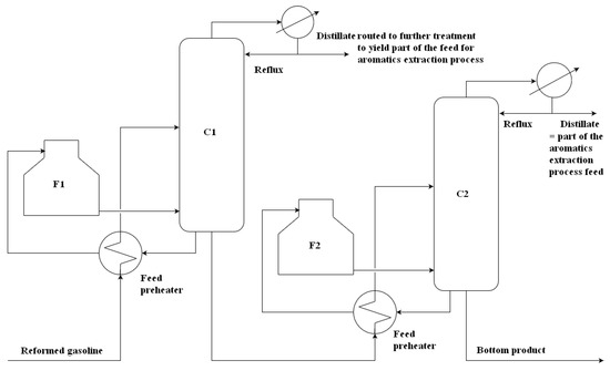
Figure 3.
Part of feed pretreatment in the aromatics fractionation process.

Table 1.
Basic parameters of feed pretreatment columns.
Aromatics-rich feed from the pretreatment unit and other sources pass through an extraction column where the aromatics and nonaromatic hydrocarbons are separated. Solvent regeneration yields an aromatic fraction containing BTX and higher aromatics. Subsequent fractionation in rectification columns yields high-purity benzene and high-purity toluene. Solvent regeneration column and columns providing benzene and toluene are reboiled by steam reboilers. Separation of the remaining xylenes, ethylbenzene, and higher aromatics is performed in further columns reboiled by a fuel gas-fired furnace. A part of the C8+ aromatics splitting process is depicted in Figure 4. Basic information essential for the analyzed process assessment is provided in Table 2.
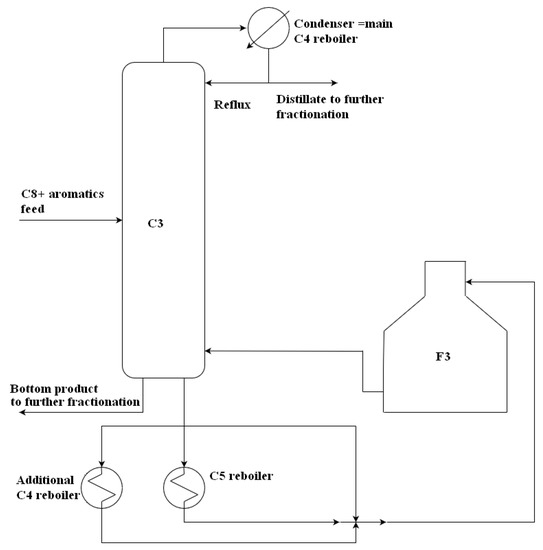
Figure 4.
Part of the C8+ aromatics splitting process.
Table 2.
Basic parameters of C8+ aromatics splitting columns.
Furnaces F1 to F3 are positioned next to each other, using the same combustion air and flue gas system, and are fed by the same fuel gas. Combustion air preheated to above 100 °C is employed as a commonly used measure for decreasing the fuel consumption and increasing the furnace efficiency in the industrial sphere [49]. As seen in Table 1 and Table 2, temperatures in reboilers allow for switching to high pressure (3.5 MPa (abs)) as the process heat source.
High-pressure steam is produced both in the refinery and in the CHP unit, the latter serving as a marginal high-pressure steam source. Apart from the high-pressure steam, the CHP unit produces 1.1 MPa (abs) and 0.5 MPa (abs) steam as well. The electric energy cogenerated in the CHP unit decreases the amount of electric energy that needs to be purchased from the external grid.
2.3. Calculations
2.3.1. Process Model
Available process data in the form of daily averages for a one-year period included:
- RFG composition and its consumption in F1, F2 and F3;
- Mass flow of combustion air delivered to F1, F2 and F3 and its temperature after preheating;
- The oxygen molar fraction in dry flue gas exiting each furnace;
- Volumetric flows of column feeds, distillates, bottom products, and reflux streams, including their temperatures;
- Volumetric flows of hot streams used in C4 and C5 reboilers and their temperature at the reboiler exit.
Additional model input data obtained from the literature included:
- The lower heating value of RFG constituents [50];
- Average specific isobaric heat capacities, specific heats of evaporation, and densities of pure compounds calculated using data from [50];
- Heat losses from the furnace’s surface to the ambient air, which amounted to 2% of the furnace design heat load according to the available documentation.
Model assumptions included:
- Complete fuel combustion in furnaces;
- Constant, representative composition of individual process streams, resulting in constant representative values of their densities, specific isobaric heat capacities, and specific heats of evaporation;
- Combustion air of zero humidity;
- Negligible heat losses from process equipment, excluding the furnaces;
- Negligible contribution of process pumps to the process energy balance.
All these data enabled us to calculate a furnace’s heat duty both from the process and the furnace side, thereby avoiding the possible inaccuracies introduced by the available short-cuts [51].
Representative process streams’ composition and temperature, along with the resulting representative densities and specific heats of evaporation, are provided in Table 3 and Table 4. Process data are covered by a nondisclosure agreement with the refinery and thus cannot be made available to the public.
Table 3.
Representative composition and physical properties approximation for C1,2 process streams. Nonaromatics are represented by n-pentane; C9+ aromatics are represented by propylbenzene.
Table 4.
Representative composition and physical properties approximation for C3 process streams. C9+ aromatics are represented by propylbenzene.
2.3.2. CHP Unit
The simplified CHP unit layout is presented in [52]. The marginal thermal efficiency of the CHP unit was estimated to be 85%, considering stack losses and other heat, water, and steam losses. This is in good agreement with the reference thermal efficiency of 86% (1.16 GJ fuel energy per 1 GJ net heat in steam exported) for a 110 MWe power plant block, as stated in Ibler et al. [41]. The CHP unit has an installed power production capacity of over 100 MWe, justifying this thermal efficiency comparison. The average value of the HFO lower heating value considered is 40.5 MJ/kg. The steam enthalpy of the 3.5 MPa (abs) steam exported from the CHP unit is 3.1 MJ/kg (3.5 MPa (abs), 350 °C), yielding specific HFO consumption of 0.09 tHFO/tsteam, used to convert steam production change to fuel consumption change, as in Equation (27).
A marginal amount of electric energy cogenerated in the CHP unit by steam expansion in steam turbines, sBP, is shown in Table 5 and applied in Equation (28) to calculate the change in the CHP unit backpressure power output as an adiabatic steam expansion enthalpy difference [42,43]; the value obtained agrees well with the CHP unit’s operational experience. The approximation by linear dependence of steam turbine power production on mass flow of expanding steam [41,42,43,44] means that this marginal parameter is constant regardless of the turbine load.
Table 5.
Marginal backpressure electric energy production in the CHP unit, eBPR,p, in kWh per t of expanding steam to p-th pressure level, estimated with the turbine model from [42].
Parameter α in Equation (28) is 0.05; see Equation (17). The CHP unit’s summer operational mode differs somewhat from that during the rest of the year. A decreased low-pressure steam demand in summer leads to lower electric energy production. The lower acceptable power production limit is 35 MW, which ensures that the most critical production units in the refinery remain in operation in case of an external electric grid blackout. If less backpressure electric energy is produced, the condensing turbines have to produce the required amount of electric energy. A change in the backpressure electric energy production thus leads to an opposite change in the condensing power production, yielding zero power production change. Fuel oil consumption is then modified to yield Equation (29):
Parameter 3 MWh/tHFO represents the marginal condensing power production from heavy fuel oil in the CHP unit, as reported by the refinery. Current climatic conditions are shifting toward shorter winters and longer and hotter summers, which will increase the share of “summer” conditions to 40% of the annual CHP unit operating time.
2.3.3. Model Scenarios
Four different scenarios were considered with regard to the actual and envisioned future refinery and CHP unit operation, as well as the possibilities of heat conservation.
Scenario A. Represents the current refinery and CHP unit operation as described above and serves as the base case. Heat in hot steam condensates remains without utilization.
Scenario B. Modification of A. Improved condensates heat recovery is considered via coupled condensates flashing to low-pressure level and cooling to 120 °C. Less HPS and LPS steam has to be produced in the CHP unit, leading to lower HFO consumption as well as reduced backpressure electricity production compared to in A.
Scenario C. Modification of A to reflect possible HPS excess in the future due to envisioned investment projects in the refinery. HPS is throttled down to MPS level. HPS utilization in steam reboilers eliminates the need for steam throttling and increases backpressure power production in the CHP unit compared to A.
Scenario D. Modification of B by considering the hot steam condensates returned to the CHP unit. Further HFO consumption and power production decrease in the CHP unit compared to B are anticipated. CHTW import to the CHP unit decreased.
2.3.4. Environmental Assessment
The Slovakian regulation Nr. 410/2012, Annex 4 [53] defines the following conditions for comparing pollutant emissions from emission sources fired with various fuels:
- dry flue gas, complete combustion, 3 vol % O2 content in dry flue gas both for refinery fuel gas and heavy fuel oil;
- pollutant emissions expressed in mg/mn3.
Material balances of the combustion processes for a representative composition of RFG and HFO yielded the results shown in Table 6. The lower heating value of the RFG, based on its representative composition, is 45.1 MJ/kg.
Table 6.
Results of fuel combustion material balance.
The flue gas produced in the CHP unit boilers passes through a sulfur oxide removal process before being emitted through the stack [54,55]. Flue gas desulphurization efficiency of around 80% is achieved [54]. Other pollutants in the flue gas include nitrogen oxides, NOx, carbon monoxide, CO, and solid particles (particulate matter, PM). Emission protocols provide information about the pollutants content in flue gases from both refinery furnaces and CHP unit boilers [56,57,58]; their relevant values are provided in Table 7. The three-year averages were used in further calculations.
Table 7.
a. Pollutant concentrations in flue gas from refinery furnaces [56,57,58]; *—recalculated to specific emission, sem,RFG, using specific dry flue gas production from RFG combustion listed in Table 6. b. Pollutant concentrations in flue gas from CHP unit boilers [56,57,58]; *—recalculated to specific emission, sem,HFO, using specific dry flue gas production from HFO combustion listed in Table 6.
Specific pollutant emissions from RFG and HFO combustion, sem,RFG, and, sem,HFO, in g/kgfuel (listed in Table 7) were used to calculate the annual emissions balance change of individual pollutants resulting from a change in the process heat source for columns C1 to C5.
Electric energy cogenerated in the CHP unit lowers the amount of electric energy that must be purchased from the external grid and thus decreases the corresponding pollutant emissions from power plants. Slovenské elektrárne, a.s, is the major energy producer in Slovakia. Table 8 presents the specific emissions from electric energy production by Slovenské elektrárne, a.s., calculated from the data in the 2016 and 2017 annual reports [59,60]. Their two-year average is employed in further calculations.
Table 8.
Specific emissions from electric energy production, sem,el, produced by Slovenské elektrárne, a.s. and related to the net electric energy delivery to the grid [59,60].
2.3.5. Economic Assessment
Both steam and RFG cost are expressed in €/GJ. An economic assessment included the impact of their variations on the project payback period. Variations in the range of €4–10/GJ were assumed, with the steam cost ranging from 75% to 100% of that of RFG. Transposition of this interval to HFO and RFG yielded an HFO cost of €162–405/tHFO and an RFG cost of €180–451/tRFG.
The carbon dioxide emissions cost variation interval considered was €10–30/t. For simplicity, the cost of all the other pollutants was set to €66.3/t, which equals that of SO2 emissions set by Slovak legislation [61].
The electric energy cost was assumed to vary between €40 and 100/MWh. The cost of chemically treated water imported by the CHP unit was €0.6/t. In this study, 8000 working hours per year were assumed for the analyzed processes. In total investment cost (TIC) estimation, a procedure from the literature [48] was applied. Key equipment sizing proceeded as follows:
Reboilers: Design heat duty, , was obtained as the calculated maximum process heat duty multiplied by a factor of 1.2 to allow for a possible intensification process in the future. The overall heat transfer coefficient, U = 700 W(m−2.K−1), was used in the heat transfer equation, Equation (28), in which the applied value of U represents the average of higher hydrocarbons’ reboiling by condensing water steam [48]. The logarithmic mean temperature difference, LMTD, was reduced in the case of boiling liquid/condensing steam to a simple temperature difference between these two fluids. The condensing HPS temperature, tcondens,HPS, was estimated at a steam pressure of 3.3 MPa (abs) to include the inevitable steam pressure losses in the system. The hydrocarbon boiling temperature, tboil,HC, used in calculations is the maximum observed hydrocarbon steam temperature at the discharge of individual process furnaces over a period of one year.
The resulting reboiler heat transfer surface, , from Equation (30) was divided in two, assuming that two identical reboilers are to be installed and operated simultaneously to comply with the best practice in the refinery. If exceeds 1000 m2, it can be divided into four identical reboilers. While installing multiple reboilers instead of a large single one is more costly, it allows for their individual cleaning without the need to interrupt the production process.
Condensate cooler: The applied procedure is similar; U = 400 W(m−2·K−1) was assumed in this application.
Pumps: Design steam condensate flow from condensates collection tank results from steam consumption in the reboilers, as shown in Figure 5. Two positions were assumed to allow for uninterrupted process operations during pump breakdown. Steam desuperheating pumps’ sizing was based on the anticipated HPS consumption and a temperature of 350 °C before desuperheating. Slightly superheated steam conditions (saturation temperature +10 °C) were reached. Low-pressure steam condensate from the condensates collection tank was used as the desuperheating agent.
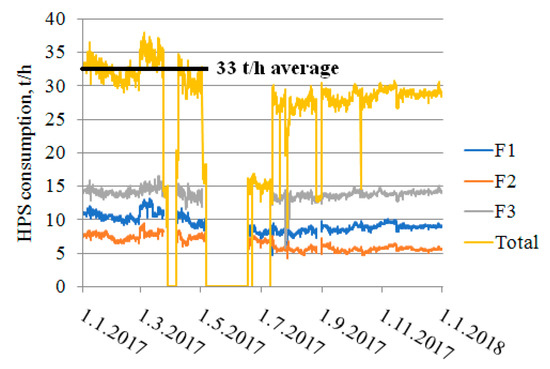
Figure 5.
HPS steam consumption, calculated to cover the process heat duty currently covered by furnaces F1 to F3.
The obtained key equipment cost was then further adjusted by including the equipment pressure factor and recalculated to the 2020 price level from the 2002 base price level used in [48] by the CEPCI index. The resulting equipment cost was then converted to TIC by applying suitable Lang factors [48]. A simple payback period was calculated by dividing the TIC by the annual benefit, obtained from Equation (23).
3. Results and Discussion
3.1. Model Verification
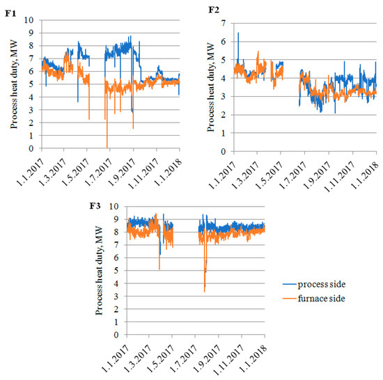
Process heat duty calculation model verification (Equations (1)–(11)) is presented in Figure 6. As can be seen, the process heat duties calculated from the process and furnace side correlate well, with only a few exceptions. A discussion with plant operators revealed that major discrepancies correlate with process flowmeters’ (reflux flow) calibration. A better match can be seen during higher process heat load periods. The highest observed heat loads were multiplied by a factor of 1.1 to 1.3 after discussions with plant engineers to provide some margin for possible future plant intensification. The adjusted maximal heat loads gave indications for new reboilers’ sizing.
Verified process heat duties were used to estimate HPS consumption in individual reboilers. An average total steam consumption of 33 t/h was used in the following economic calculations, which corresponds to the situation in the first months in 2017 and is expected to occur much more often in the future. A peak HPS consumption of 38 t/h or over can be anticipated to occur from time to time, and consequently the steam pipeline capacity has to be revised. HPS is delivered to the considered production units via a steam pipeline with an internal diameter of 150 mm, which is insufficient for the transport of even the average HPS flow to new reboilers. A new pipeline with an internal diameter of 200 mm has to be installed to ensure HPS delivery to new reboilers without excessive pressure loss; the approximate pipeline length is 100 m. The costs associated with the extra HPS pipeline are included in the TIC calculation, discussed below.
3.2. Investment Scope and Cost
Table 9 details the TIC estimation procedure for scenario B. The resulting TIC estimate of over €4 million indicates that to reach a payback period appropriate for the refinery (less than four years), the yearly benefit has to exceed €1.1 million/year. The Lang factor value for “Piping installed” of 80% was higher than the recommended value of 68% in [48] to cover the extra costs associated with the new HPS pipeline instalment.
Table 9.
Total investment cost estimate based on [48] for scenario B.
The TIC estimation for other scenarios proceeded similarly and the results are presented in Table 10. Scenarios A and C produced an identical TIC, lower than in B due to the absence of condensate coolers. Scenario D requires a higher TIC than B as it requires a new condensates return pipeline to the CHP unit with a length of several hundred meters. Its cost was estimated to be €450,000 after plant engineers considered the past investment costs of similar projects.
Table 10.
Total investment cost for scenarios A–D.
The installation of new steam reboilers and shutting down old, inefficient furnaces reduced the future expenses associated with equipment maintenance and with the necessary adjustment of furnaces and burners to tighter emission limits. Another, though even less tangible, benefit is the contribution of this investment to a decreased fire and explosion risk in an aromatics production plant.
3.3. Emissions Balances
For scenario A the calculated annual pollutant balance in the refinery is shown in Table 11. As can be seen, changes in all other pollutant emissions, except for CO2, are fairly low, which seems surprising considering that refinery fuel gas is much “cleaner” fuel than the heavy fuel oil combusted in the CHP unit boilers. This accentuates the need to evaluate emissions from fuel combustion not just using the “clean–dirty” fuel concept, but also by taking into account the operation of individual thermal aggregates where fuel is combusted.
Table 11.
Annual pollutant balance in the refinery for Scenario A.
The following facts elucidate the observed small changes in pollutant emissions:
- Furnaces F1 to F3 are of advanced age, including the RFG burners installed within. Their renovation is necessary to meet stricter emission limits.
- Compared to CHP unit steam boilers, no flue gas cleaning is installed in the common flue gas ducts from F1, F2, and F3. CHP unit boilers are equipped with dedusting, deSOx, and deNOx systems, which significantly reduce pollutant emissions from the CHP unit.
Carbon dioxide emissions, on the other hand, increase significantly, probably due to the high specific HFO consumption per t of exported steam, as no steam condensates are returned to the CHP unit in scenario A. Lower CO2 emissions can be expected in other scenarios.
Table 12 compares the pollutant emissions from individual scenarios and elucidates the influence of incorporating emissions from power generation in emissions estimation. Emissions from power generation were estimated using the specific emission factors listed in Table 8. As expected, the CO2 emissions increase is lower in all other scenarios compared to scenario A. Scenarios B and D do not consume that much HFO in the CHP unit compared to scenario A and produce a comparable electric energy amount in the CHP unit, e.g., the refinery itself produces fewer emissions. Substantially more electric energy is cogenerated in the CHP unit in scenario C, which reduces CO2 emissions from the CHP unit in the summer operation regime (see Equation (29)). A CO2 emissions decrease was achieved outside the refinery in the CHP winter operation regime. Similarly, the SO2 emissions increase in scenario C was cut in half compared to scenario A for the same reason. This effect is less pronounced in other pollutants, but it still exists.
Table 12.
Total pollutant balance, taking into account the electric energy cogenerated in the CHP unit in Scenarios A to D.
Applying marginal emission factors instead of the average ones from the chosen energy mix significantly improved the pollutant emission amount estimate accuracy [62]. Slovenské elektrárne, a.s. operates several hydropower and nuclear power plants, which contribute to the low energy mix emission factors (Table 8). Such power plants, however, cannot be considered traditional marginal power sources, e.g., power sources with flexible operation. This function can be met, for instance, by a flexible NG-based combined cycle power plant. Assuming a net electric efficiency of 50%, its CO2 emission factor is over 400 kgCO2/MWh, i.e., it triples the value listed in Table 8. Coal- or oil-fired power is a marginal power source with an even higher CO2 emission factor: up to 900 kgCO2/MWh [63] and generally higher emission factors of other pollutants compared to those used in this study. Table 13 shows the impact of an emissions factor considered marginal for power production on the total CO2 balance in individual scenarios.
Table 13.
Impact of electric energy production emissions factor on the total CO2 balance in individual scenarios.
The results presented in Table 13 highlight the significance of correct power production emission factor selection: annual CO2 emissions decrease by up to 45% (scenario C) when using the coal power plant factor instead of that of Slovenské elektrárne, a.s. In other scenarios, the effect is less pronounced, but the difference can still exceed 15% (scenarios A and B). Scenario D is the least sensitive to the power production emission factor selection as it leads to the lowest power production increase in the CHP unit compared to the present state. Similar results can also be expected for other pollutants’ balances. This stresses the need for emissions from power production to be included in the total emissions balance, together with the proper use of the power production emissions factor.
3.4. Economics and Sensitivity Analysis
An economic assessment of individual scenarios is provided in Figure 7 and Table 14. Annual benefit changes with heat in steam price to heat in RFG ratio (herein referred to as the Ratio), as well as with electric energy cost, are investigated in Figure 7. These two factors mostly influence the economic attractiveness of individual scenarios. The annual benefit of scenario A is negative in all cases with a Ratio value of 90% or over, whereas all other scenarios provide a positive annual benefit under these conditions. This effect can be attributed to the decreased HFO consumption compared to scenario A (scenarios B and D) or to the much higher power production in the CHP unit compared to scenario A (scenario C). Therefore, scenarios B and D are much less sensitive to electric energy price changes than scenario C. Of all the scenarios considered, D is the most robust one, leading to positive annual benefits in all cases.
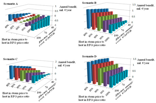
Figure 7.
Benefit sensitivity to key economic variables; base case definition: cRFG = €7/GJ, cCO2 = €10/t, cCHTW = €0.6/t. Scenarios A to D are defined in the Model scenarios subchapter.
Table 14.
Sensitivity analysis of benefit change; base case definition: cRFG = €7/GJ, csteam = 0.8. cRFG, cCO2 = €10/t, cel = €70/MWh, cCHTW = €0.6/t.
The influence of other factors’ changes on the annual benefit is shown in Table 14. The cost of carbon dioxide emissions can be identified as the third most important factor. Its increase from €10 to €20/t reduces the annual benefit in all scenarios; A and C are the most sensitive to this change.
The annual benefit of scenario A reaches a negative value under these conditions and the simple payback periods of scenarios B and C increase to four years or more. Only scenario D is sufficiently attractive, even with a carbon dioxide emissions price of up to €30/t, leading to an annual benefit of around €1.2 million/year and to the simple payback period being slightly longer than four years. The sensitivity of all scenarios to carbon dioxide emissions’ price increase has to be accounted for, especially since refinery managers expect emissions prices to increase to €30/t or above in the near future.
As can further be seen, the RFG cost increase and chemically treated water cost decrease are beneficial in all scenarios, with scenario D being the most sensitive to RFG cost change and scenarios A and C to most sensitive CHTW cost change. RFG cost is an important factor influencing the economics of the scenarios; RFG cost changes of ±10% are quite common within the time span of a few months. CHTW cost changes are less frequent and less pronounced, and therefore this factor can be considered the least important.
Examination of other pollutant costs’ variation in terms of the annual benefit of the considered scenarios seems to be meaningless. Their total increase is below 100 t/year (scenario A), which means that even doubling their cost (from €66 to €132/t) decreases the annual benefit by less than €10,000/year.
4. Conclusions
The complex framework of process heat source switching in refinery conditions developed in this study allows for its objective assessment from energy, environmental, and economic points of view. The effect on other refinery parts as well as on emissions from the power production process outside the refinery was also taken into account.
The method of process heat source switching was tested on an aromatics production plant, employing higher boiling hydrocarbons fractionation in columns reboiled by refinery fuel gas-fired furnaces. Reboiling by condensing the high-pressure steam produced in the CHP unit in heavy fuel oil-fired steam boilers was proposed. The scenarios considered reflect the possibilities for improved heat conservation in the plant itself, condensates return to the CHP unit, as well as possible future high-pressure steam throttling mitigation.
The annual benefits resulting from individual scenarios exhibit various sensitivity to the key economic parameters change, which further stresses the need for complex method application in the process of heat source switching. Apart from fuel and steam costs, which are the most important economic parameters, energy costs and carbon dioxide emission costs were identified as other parameters to which the annual benefit is sensitive. The most robust scenario incorporates both heat conservation and condensates return to the CHP unit, and, despite it having the highest estimated total investment cost (of over €4.5 million), it offers acceptable, simple payback periods in most energy and media costs combination cases.
An environmental evaluation revealed that taking into account the emissions generated in the power production process outside the refinery can substantially change the estimate of the total generated emissions. Apart from CO2, the emissions of other pollutants did not increase as significantly as expected when switching from refinery fuel gas to heavy fuel oil. The reason is that refinery fuel gas-fired furnaces are small and medium-sized thermal aggregates with no flue gas cleaning installed, while the CHP unit steam boilers are equipped with multistage flue gas cleaning. The operational conditions and technical state of thermal aggregates are thus as important as the fuel type they consume in a complex emissions generation assessment. These findings are relevant and should result in more complex emissions generation evaluation in industrial process heat source switching projects.
It can be concluded that complex multi-objective evaluation is necessary for industrial heat source switching projects and the use of “cleaner” fuels is not the only goal to be pursued. The presented method is a suitable tool for such evaluations and can thus be applied in the industry generally to aid engineers, energy managers, and industrial policy makers with their decision-making.
Author Contributions
Contributions of individual authors: Conceptualization: M.V., D.J., and P.I.; data curation: D.J. and M.L.; funding acquisition: M.V., J.K., and L.L.; investigation: D.J. and M.L.; methodology: M.V. and P.I.; resources: P.I. and M.L.; software: J.J.; visualization: J.J.; writing—original draft: M.V. and D.J.; writing—review and editing: J.J., J.K., and L.L.
Funding
This work was financially supported by the Slovak Scientific Agency, Grant No. VEGA 1/0659/18 and the Slovak Research and Development Agency, Grant Nos. APVV-15-0148 and APVV-18-0134.
Acknowledgments
The authors would like to express their thanks to all the SLOVNAFT, a.s., employees who contributed to the final scope and form of this paper. The authors owe special thanks to Barbora Dudášová for language checking.
Conflicts of Interest
The authors declare no conflict of interest.
Nomenclature
| Symbols and abbreviations | ||
| A | heat transfer surface | (m2) |
| (annual) benefit | (€/year) | |
| BP | backpressure (electric energy production) | |
| BTX | benzene–toluene–xylene fraction | |
| C | column (rectification column) | |
| (annual) costs | (€/year) | |
| c | specific cost (fuel, electric energy); fee (pollutant) | (€/unit) |
| C8+ | hydrocarbons with eight or more carbon atoms in the molecule | |
| C9+ | hydrocarbons with nine or more carbon atoms in the molecule | |
| cP | specific isobaric heat capacity | (kJ/kg/K) |
| eBPR | marginal backpressure electric energy production | (kWh/t) |
| F | furnace | |
| GHG | greenhouse gases | |
| enthalpy flux | (GJ/h, MW) | |
| HFO | heavy fuel oil | |
| HPS | high pressure steam (3.5 MPa (abs.)) | |
| HX | heat exchanger | |
| CHP | combined heat and power unit | |
| LHV | lower heating value | (MJ/kg) |
| LHVv | volumetric lower heating value | (MJ/m3) |
| LPS | low pressure steam (0.5 MPa (abs.)) | |
| M | molar mass | (g/mol) |
| mass flow | (kg/h; t/h) | |
| MPS | middle pressure steam (1.1 MPa (abs.)) | |
| N | normal (normal conditions = 0 °C and 101.325 kPa) | |
| NG | natural gas | |
| OECD | Organization for Economic Co-operation and Development | |
| P | power output | (kW, MW) |
| PM | particulate matter | |
| heat flux | (kW, MW) | |
| RFG | refinery fuel gas | |
| ST | steam turbine | |
| sem | specific emissions of pollutants | (g/kgfuel) |
| t | temperature | (°C) |
| TIC | total investment cost | |
| U | overall heat transfer coefficient | (W/m2/K) |
| VHPS | very high-pressure steam (9 MPa (abs.)) | |
| v | specific dry flue gas volume | (mn3/kgfuel) |
| w | component weight fraction | |
| WTU | water treatment unit | |
| x | component molar fraction | |
| ∆tLM | logarithmic mean temperature difference | (K) |
| ∆vaph | specific enthalpy of vaporization | (kJ/kg) |
| Subscripts | ||
| air | combustion air | |
| amb | ambient (conditions) | |
| boil | boiling (temperature) | |
| BP | bottom product | |
| c | c-th column | |
| CHP | (related to) combined heat and power unit | |
| CHTW | chemically treated water | |
| circ | circulating | |
| cond | condensate | |
| condens | condensing (temperature) | |
| D | distillate | |
| des | design | |
| el | electric (energy) | |
| em | emissions (related to) | |
| F | furnace | |
| FG | flue gas | |
| flash | flash (steam) | |
| FS | furnace-side (heat duty calculation) | |
| fuel | (related to) fuel | |
| HC | hydrocarbon (stream) | |
| i | i-th component | |
| in | inlet (stream) | |
| j | j-th stream | |
| k | k-th furnace | |
| (l) | liquid | |
| m | molar | |
| marg | marginal | |
| n | pollutant; n = SO2, CO, PM, NOx, CO2 | |
| out | outlet (stream) | |
| overall | overall (emissions) | |
| ovhd | overhead (vapors leaving rectification column) | |
| p | p-th steam pressure level (HPS, MPS, LPS) | |
| preheat | combustion air preheat (temperature) | |
| PS | process-side (heat duty calculation) | |
| r | r-th fuel | |
| R | reflux | |
| REB | reboiling (temperature) | |
| REF | reference (state) | |
| refinery | (related to) refinery | |
| summer | (related to) summer conditions | |
| t | thermal | |
| tot | total | |
| Greek symbols | ||
| α | own electric energy consumption coefficient | |
| γ | pollutant concentration in flue gas | (mg/mn3) |
| η | efficiency | (-) |
| ρ | density | (kg/m3) |
| φ | excess chemically treated water import coefficient | |
References
- Energy Information Administration. International Energy Outlook 2016; Energy Information Administration: Washington, DC, USA; Department of Energy: Cebu City, The Philippines, 2016. Available online: https://www.eia.gov/outlooks/ieo/pdf/0484(2016).pdf (accessed on 15 January 2019).
- Worell, E.; Corsten, M.; Galitsky, C. Energy Efficiency Improvement and Cost Saving Opportunities for Petroleum Refineries. An ENERGY STAR® Guide for Energy and Plant Managers. A document prepared for The United States Environmental Protection Agency; 2015. Available online: www.energystar.gov/industry (accessed on 4 June 2018).
- Kosobokova, E.M.; Berezinets, P.A. Developing an energy-saving strategy at oil refineries. Chem. Technol. Fuels Oils 2001, 37, 5–8. [Google Scholar] [CrossRef]
- Alhajji, M.; Demirel, Y. Energy and environmental sustainability assessment of a crude oil refinery by thermodynamic analysis. Int. J. Energy Res. 2015, 39, 1925–1941. [Google Scholar] [CrossRef]
- Li, J.; Xiao, X.; Boukouvala, F.; Floudas, C.A.; Zhao, B.; Du, G.; Su, X.; Liu, H. Data-Driven Mathematical Modeling and Global Optimization Framework for Entire Petrochemical Planning Operations. AIChE J. 2016, 62, 3020–3040. [Google Scholar] [CrossRef]
- Rehfelt, M.; Fleiter, T.; Worrell, E. Inter-fuel substitution in European industry: A random utility approach on industrial heat demand. J. Clean. Prod. 2018, 187, 98–110. [Google Scholar] [CrossRef]
- Ameri, M.; Mokhtari, H.; Sani, M.M. 4E analyses and multi-objective optimization of different fuels application for a large combined cycle power plant. Energy 2018, 156, 371–386. [Google Scholar] [CrossRef]
- Szklo, A.; Schaeffer, R. Fuel specification, energy consumption and CO2 emission in oil refineries. Energy 2007, 32, 1075–1092. [Google Scholar] [CrossRef]
- Morrow, W.R., III; Marano, J.; Hasanbeigi, A.; Masanet, E.; Sathaye, J. Efficiency improvement and CO2 emission reduction potentials in the United States petroleum refining industry. Energy 2015, 93, 95–105. [Google Scholar] [CrossRef]
- Al-Rowaili, F.N.; Ba-Shammakh, M.S. Maximisation of an oil refinery profit with products quality and NO2 constraints. J. Clean. Prod. 2017, 165, 1582–1597. [Google Scholar] [CrossRef]
- Berghout, N.; Meerman, H.; van den Broek, M.; Faaij, A. Assessing deployment pathways for greenhouse gas emissions reductions in an industrial plant—A case study for a complex oil refinery. Appl. Energy 2019, 236, 354–378. [Google Scholar] [CrossRef]
- Gharaie, M.; Panjeshahi, M.H.; Kim, J.-K.; Jobson, M.; Smith, R. Retrofit strategy for the site-wide mitigation of CO2 emissions in the process industries. Chem. Eng. Res. Des. 2015, 94, 213–241. [Google Scholar] [CrossRef]
- Schneider, D.R.; Bogdan, Ž. Effect of heavy fuel oil/natural gas co-combustion on pollutant generation in retrofitted power plant. Appl. Therm. Eng. 2007, 27, 1944–1950. [Google Scholar] [CrossRef]
- Seljeskog, M.; Sevault, A.; Ditaranto, M. Pursuing the oxy-fuel light-/heavy oil retrofit route in oil refineries-A small scale retrofit study. Energy Procedia 2013, 37, 7231–7248. [Google Scholar] [CrossRef]
- Escudero, A.I.; Espatolero, S.; Romeo, L.M. Oxy-combustion power plant integration in an oil refinery to reduce CO2 emissions. Int. J. Greenhouse Gas Control 2016, 45, 118–129. [Google Scholar] [CrossRef]
- Dzurňák, R.; Varga, A.; Kizek, J.; Jablonský, G.; Lukáč, L. Influence of Burner Nozzle Parameters Analysis on the Aluminium Melting Process. Appl. Sci. 2019, 9, 1614. [Google Scholar] [CrossRef]
- Tumanovskii, A.G.; Kosobokova, E.M. Secondary energy carriers in oil refineries. Chem. Technol. Fuels Oils 2001, 37, 73–77. [Google Scholar] [CrossRef]
- Zhou, L.; Liao, Z.; Wang, J.; Jiang, B.; Yang, Y.; Du, W. Energy configuration and operation optimization of refinery fuel gas networks. Appl. Energy 2015, 139, 365–375. [Google Scholar] [CrossRef]
- Fonseca, A.; Tavares, M.L.C.; Gomes, L.A.C.N. Burning clean fuel gas improves energetic efficiency. Energy Convers. Manag. 2010, 51, 498–504. [Google Scholar] [CrossRef]
- Variny, M.; Blahušiak, M.; Mierka, O.; Godó, Š.; Margetíny, T. Energy saving measures from their cradle to full adoption with verified, monitored, and targeted performance: A look back at energy audit at Catalytic Naphtha Reforming Unit (CCR). Energy Effic. 2019, in press. [Google Scholar] [CrossRef]
- Ruan, X.; Xiao, H.; Jiang, X.; Yan, X.; Dai, Y.; He, G. Graphic synthesis method for multi-technique integration separation sequences of multi-input refinery gases. Sep. Purif. Technol. 2018, 214, 187–195. [Google Scholar] [CrossRef]
- Comodi, G.; Renzi, M.; Rossi, M. Energy efficiency improvement in oil refineries through flare gas recovery technique to meet the emission trading targets. Energy 2016, 109, 1–12. [Google Scholar] [CrossRef]
- Zhang, J.D.; Rong, G. An MILP model for multi-period optimization of fuel gas system scheduling in refinery and its marginal value analysis. Chem. Eng. Res. Des. 2008, 86, 141–151. [Google Scholar] [CrossRef]
- Jiandong, Z.; Gang, R.; Weifeng, H.; Chenbo, H. Simulation based approach for scheduling of fuel gas system in refinery. Chem. Eng. Res. Des. 2010, 88, 87–99. [Google Scholar]
- Lee, C.-L.; Jou, C.-J.G.; Tsai, C.-H.; Wang, H.P. Improvement in the performance of a medium-pressure-boiler through the adjustment of inlet fuels in a refinery plant. Fuel 2007, 86, 625–631. [Google Scholar] [CrossRef]
- Lee, C.-L.; Hou, S.-S.; Lee, W.-J.; Jou, C.-J.G. Improving cost effectiveness for the furnace in a full-scale refinery plant with reuse of waste tail gas fuel. Int. J. Hydrogen Energy 2010, 35, 1797–1802. [Google Scholar] [CrossRef]
- Gabr, E.M.; Mohamed, S.M.; El-Temtamy, S.A.; Gendi, T.S. Application of energy management coupled with fuel switching on a hydrotreater unit. Egypt. J. Pet. 2016, 25, 65–74. [Google Scholar] [CrossRef]
- Gatfaoui, H. Pricing the (European) option to switch between two energy sources: An application to crude oil and natural gas. Energy Policy 2015, 87, 270–283. [Google Scholar] [CrossRef]
- Ditaranto, M.; Anantharaman, R.; Weydahl, T. Performance and NOx emissions of refinery fired heaters retrofitted to hydrogen combustion. Energy Procedia 2013, 37, 7214–7220. [Google Scholar] [CrossRef]
- Frangopoulos, C.A.; Lygeros, A.I.; Markou, C.T.; Kaloritis, P. Thermoeconomic operation optimization of the Hellenic Aspropyrgos refinery combined-cycle cogeneration system. Appl. Therm. Eng. 1996, 16, 949–958. [Google Scholar] [CrossRef]
- Rahimpour, M.R.; Jokar, S.M. Feasibility of flare gas reformation to practical energy in Farashband gas refinery: No gas flaring. J. Hazard. Mater. 2012, 209, 204–217. [Google Scholar] [CrossRef]
- Rahimpour, M.R.; Jamshidnejad, Z.; Jokar, S.M.; Karimi, G.; Ghorbani, A.; Mohammadi, A.H. A comparative study on three different methods for flare gas recovery of Asalooye Gas Refinery. J. Nat. Gas Sci. Eng. 2012, 4, 17–28. [Google Scholar] [CrossRef]
- Zargaran, J.; Bahmani, M. Simulation of separation of valuable components from Tehran refinery flare stack gases. Pet. Coal 2011, 53, 78–83. [Google Scholar]
- Ghasemikafrudi, E.; Amini, M.; Habibi, M.R.; Hassankiadeh, Q.D. Environmental effects and economic study on flare gas recovery for using as fuel or feedstock. Pet. Coal 2017, 59, 18–28. [Google Scholar]
- Lowe, C.; Brancaccio, N.; Batten, D.; Leung, C.; Waibel, D. Technology Assessment of Hydrogen Firing of Process Heaters. Energy Procedia 2011, 4, 1058–1065. [Google Scholar] [CrossRef][Green Version]
- Weydahl, T.; Jamaluddin, J.; Seljeskog, M.; Anantharaman, R. Pursuing the pre-combustion CCS route in oil refineries—The impact on fired heaters. Appl. Energy 2013, 102, 833–839. [Google Scholar] [CrossRef]
- Vilarinho, A.N.; Campos, J.B.L.M.; Pinho, C. Energy and exergy analysis of an aromatics plant. Case Stud. Therm. Eng. 2016, 8, 115–127. [Google Scholar] [CrossRef]
- Mierka, O.; Variny, M. A study on utilization improvement of cogeneration potential in a complex industrial steam and power plant. In Power Engineering 2012 Proceedings of the Energy-Ecology-Economy 10th International Scientific Conference IEEE 2012, Tatranske, Matliare (Slovakia), 15–17 May 2012; Slovak University of Technology in Bratislava: Bratislava, Slovakia, 2012; ISBN 978-80-89402-49-6. [Google Scholar]
- Spirax-Sarco. The Steam and Condensate Loop. Effective Steam Engineering for Today; Spirax-Sarco Limited: Cheltenham, UK, 2011; ISBN 978-0-9550691-5-4. [Google Scholar]
- Einstein, D.; Worrell, E.; Khrushch, M. Steam Systems in Industry: Energy Use and Energy Efficiency Improvement Potentials. 2001. Available online: https://www.osti.gov/scitech/servlets/purl/789187 (accessed on 29 January 2019).
- Ibler, Z.; Karták, J.; Mertlová, J.; Ibler, Z. Technický Průvodce Energetika; Nakladatelství BEN–technická literature: Praha, Czech, 2012; ISBN 80-7300-026-1. (In Czech) [Google Scholar]
- Mavromatis, S.P.; Kokossis, A.C. Conceptual optimization of utility networks for operational variations—I. Targets and level optimization. Chem. Eng. Sci. 1998, 53, 1585–1608. [Google Scholar] [CrossRef]
- Varbanov, P.S.; Doyle, S.; Smith, R. Modelling and optimization of utility systems. Chem. Eng. Res. Des. 2004, 82, 561–578. [Google Scholar] [CrossRef]
- Chaibakhsh, A.; Ghaffari, A. Steam turbine model. Simul. Mod. Pract. Theory 2008, 16, 1145–1162. [Google Scholar] [CrossRef]
- Luo, X.; Zhang, B.; Chen, Y.; Mo, S. Modeling and optimization of utility systems containing multiple extractions steam turbines. Energy 2011, 36, 3501–3512. [Google Scholar] [CrossRef]
- Mrzljak, V.; Poljak, I.; Mrakovčić, T. Energy and exergy analysis of the turbogenerators and steam turbine for the main feed water pump drive on LNG carrier. Energy Convers. Manag. 2017, 140, 307–323. [Google Scholar] [CrossRef]
- Directive, C. Directive 2010/75/EU of the European Parliament and of the Council. Off. J. Eur. Union L 2010, 334, 17–119. [Google Scholar]
- Peters, M.S.; Timmerhaus, K.D.; West, R.E. Plant Design and Economics for Chemical Engineers, 5th ed.; McGraw-Hill: New York, NY, USA, 2003; ISBN 0-07-239266-5. [Google Scholar]
- Yeromin, A.; Yeromina, O.; Lukáč, L.; Kizek, J.; Dzurňák, R. The possibility of increasing the efficiency of temperature distribution control in reheating furnaces. Acta Montan. Slovaca 2018, 23, 175–183. [Google Scholar]
- Perry, R.H.; Green, D.W.; Maloney, J.O. Physical and Chemical Data. In Perry’s Chemical Engineers’ Handbook, 7th ed.; McGraw-Hill Professional: London, UK, 1997; ISBN 0-07-049841-5. [Google Scholar]
- Plellis-Tsaltakis, C. A shortcut procedure for calculation of process side heat duty of refinery fired heaters. Chem. Eng. Res. Des. 2017, 124, 152–158. [Google Scholar] [CrossRef]
- CHP Unit Scheme. Available online: http://www.cmep.sk/index.php/sk/teplaren. (accessed on 11 March 2019). (In Slovak).
- Slovak Regulation Nr. 410/2012 Coll. of Ministry of Environment of Slovak Republic implementing certain provisions of the Clean Air Act of 30 November 2012. Available online: https://www.zakonypreludi.sk/zz/2012-410 (accessed on 12 September 2019). (In Slovak).
- SLOVNAFT, a.s. Information about Air Protection Measures Adopted. Available online: https://slovnaft.sk/en/about-us/sustainable-development-and-hse/environmental-protection/air-protection/ (accessed on 12 March 2019).
- Flue Gas from CHP Unit Desulphurization Process Description. Available online: http://www.cmep.sk/index.php/sk/odsirenie-spalin (accessed on 12 March 2019). (In Slovak).
- SLOVNAFT, a.s. Annual Emission Report. 2016. Available online: https://slovnaft.sk/images/slovnaft/pdf/o_nas/trvalo_udrzatelny_rozvoj/informacie_o_zivotnom_prostredi/inf_verejnosti_2016_emisie.pdf (accessed on 12 March 2019). (In Slovak).
- SLOVNAFT, a.s. Annual Emission Report. 2017. Available online: https://slovnaft.sk/images/slovnaft/pdf/o_nas/trvalo_udrzatelny_rozvoj/informacie_o_zivotnom_prostredi/informacia_pre_verejnost-kvalita_ovzdusia_emisie.pdf (accessed on 12 March 2019). (In Slovak).
- SLOVNAFT, a.s. Annual Emission Report. 2018. Available online: https://slovnaft.sk/images/slovnaft/pdf/o_nas/trvalo_udrzatelny_rozvoj/informacie_o_zivotnom_prostredi/inf_verejnosti_19_emisie.pdf (accessed on 11 March 2019). (In Slovak).
- Slovenské elektrárne, a.s. Annual Report. 2016. Available online: https://www.seas.sk/data/contentlink/se-2016-annual-report-web.pdf (accessed on 11 March 2019).
- Slovenské elektrárne, a.s. Annual Report. 2017. Available online: https://www.seas.sk/data/contentlink/se-2017-annual-report.pdf (accessed on 11 March 2019).
- Slovak Regulation Nr. 401/1998 Coll of the Slovak Parliament on air pollution charges of 16 December 1998. Available online: https://www.slov-lex.sk/pravne-predpisy/SK/ZZ/1998/401/ (accessed on 12 September 2019). (In Slovak).
- Smith, C.N.; Hittinger, E. Using marginal emission factors to improve estimates of emission benefits from appliance efficiency upgrades. Energy Eff. 2019, 12, 585–600. [Google Scholar] [CrossRef]
- Variny, M.; Hruška, M.; Mierka, O. Black liquor gasification as means of efficient cogeneration technology–A model study. Waste Forum 2018, 2, 174–182. [Google Scholar]
© 2019 by the authors. Licensee MDPI, Basel, Switzerland. This article is an open access article distributed under the terms and conditions of the Creative Commons Attribution (CC BY) license (http://creativecommons.org/licenses/by/4.0/).