Article

Physics-Informed Neural Network (PINNs) for Flow Simulation in Polymer-Assisted Hot Water Flooding

1
School of Petroleum Engineering, Yangtze University, Wuhan 430100, China
2
State Key Laboratory of Low Carbon Catalysis and Carbon Dioxide Utilization, Yangtze University, Wuhan 430100, China
3
Western Research Institute, Yangtze University, Karamay 834000, China
*
Authors to whom correspondence should be addressed.
Processes 2026, 14(2), 197; https://doi.org/10.3390/pr14020197
Submission received: 19 November 2025 / Revised: 16 December 2025 / Accepted: 24 December 2025 / Published: 6 January 2026

Abstract

Polymer-assisted hot water flooding (PAHWF) is an important enhanced oil recovery technique involving strongly coupled thermal, chemical, and multiphase flow processes. Accurate prediction of water saturation, polymer concentration, and temperature evolution in PAHWF is challenging due to the highly nonlinear and multiscale governing equations. In this study, a physics-informed neural network (PINN) framework is developed for one-dimensional PAHWF simulation as a controlled benchmark system to systematically investigate PINN behavior in multiphysics-coupled problems. The PAHWF governing equations incorporating temperature- and concentration-dependent viscosity are embedded into the PINN loss function. Three progressively designed numerical examples are conducted to examine the effects of temperature normalization, network architecture (PINN-1 versus PINN-2), and network depth on training stability and solution accuracy. The results demonstrate that temperature normalization effectively mitigates gradient-scale imbalance, significantly improving convergence stability and prediction accuracy. Furthermore, the PINN-2 architecture, which employs a dedicated network for temperature, exhibits enhanced robustness and accuracy compared with the unified PINN-1 structure. Variations in network depth show limited influence on solution quality, indicating the inherent robustness of PINNs under the proposed framework. Although conventional numerical methods remain more efficient for one-dimensional forward problems, this study establishes a methodological foundation for extending PINNs to higher-dimensional, strongly coupled PAHWF simulations and inverse reservoir problems. The proposed framework provides insights into improving PINN trainability and reliability for complex enhanced oil recovery processes.

1. Introduction

Polymer-assisted hot water flooding (abbreviated as PAHWF in this paper) is a prominent enhanced oil recovery (EOR) technique that leverages the combined benefits of thermal and chemical methods to improve oil displacement efficiency in reservoirs. By co-injecting hot water and polymers, PAHWF reduces the mobility ratio, enhances sweep efficiency, and mitigates water channeling, making it particularly effective in heavy oil reservoirs and heterogeneous formations [1,2]. The success of PAHWF hinges on accurately predicting the spatial and temporal distributions of critical parameters such as fluid saturation, polymer concentration, and temperature within the reservoir. These parameters are governed by complex, coupled nonlinear partial differential equations (PDEs) that describe mass, momentum, and energy conservation. Traditional numerical methods, such as finite difference (FDM) and finite element methods (FEM), have been widely employed to solve these equations. However, these methods often encounter challenges related to high computational costs, fine discretization requirements, and the inherent nonlinearities of multiphase, multicomponent flow in heterogeneous reservoirs [3,4]. For fractured and highly heterogeneous reservoirs, advanced numerical techniques such as streamline-based simulation within the projection-based embedded discrete fracture model (pEDFM) framework have been developed to improve efficiency and accuracy [5]. Subsequent studies further extended pEDFM to anisotropic two-phase flow using hybrid TPFA–MFD formulations, highlighting the sophistication and computational cost of state-of-the-art numerical reservoir simulators [6]. Meshless numerical methods based on extended finite volume formulations have also been proposed for fractured reservoirs, reducing meshing complexity while retaining numerical accuracy [7].
In recent years, Physics-Informed Neural Networks (PINNs) have emerged as a groundbreaking approach for solving PDEs in scientific and engineering applications. PINNs integrate the governing physical laws directly into the loss function of a neural network, enabling the model to learn solutions that are consistent with the underlying physics [8]. This approach eliminates the need for extensive discretization and can handle high-dimensional and nonlinear problems efficiently [9,10]. PINNs have been successfully applied in various fields, including fluid dynamics [11], heat transfer [12], material science [13], and geophysics [14]. Their ability to solve forward and inverse problems, as well as their flexibility in incorporating complex boundary conditions, makes them particularly attractive for reservoir engineering applications [15]. Recently, hybrid quantum–classical physics-informed neural networks have also been explored for reservoir seepage equations, indicating the potential of advanced PINN variants for accelerating subsurface flow modeling and extending classical PINN frameworks [16]. In polymer-assisted thermal recovery systems, fluid flow exhibits pronounced nonlinear behavior. Specifically, after polymer addition, the aqueous phase typically shows shear-thinning non-Newtonian characteristics, with its effective viscosity depending not only on temperature but also on polymer concentration and local flow gradients [17]. In addition, the viscosities of both oil and water phases decrease significantly with increasing temperature, leading to changes in the mobility ratio between the two phases, which in turn affects front stability and displacement efficiency. In this study, these thermo–chemical coupling effects are described through empirical viscosity models incorporated into the governing equations [18,19]. Although a Darcy-based, volume-averaged two-phase flow framework is adopted, it inherently captures the quasi-non-Newtonian, nonlinearly coupled flow behavior characteristic of the PAHWF process.
In the context of reservoir flow problems, PINNs have demonstrated significant potential. For instance, they have been used to model single-phase and multiphase flow, reactive transport, and thermal recovery processes. Raissi et al. [10] pioneered the application of PINNs to fluid dynamics, showcasing their ability to solve the Navier–Stokes equations with high accuracy. Subsequent studies have extended PINNs to reservoir-scale problems, such as water flooding [20], CO2 sequestration [21], and geothermal reservoir simulations [22]. These studies highlight the advantages of PINNs in terms of computational efficiency, accuracy, and their ability to handle heterogeneous and anisotropic reservoir properties [23]. Quantum neural network models have further been investigated for CO2 sequestration prediction in saline aquifers, suggesting potential synergies between quantum computing and data-driven reservoir modeling [24]. Moreover, PINNs have been shown to outperform traditional numerical methods in scenarios where data is sparse or where rapid solutions are required [25]. In addition to PINNs, boundary-integral type neural networks (BINNs) have been proposed for modeling flow problems in homogeneous and anisotropic reservoirs, demonstrating improved efficiency by reducing the dimensionality of the governing equations [26,27]. Emerging studies have also explored quantum computing algorithms for streamline-based waterflooding simulation, aiming to accelerate large-scale reservoir flow calculations [28].
The application of PINNs to PAHWF simulations is particularly promising due to the technique’s inherent complexity. PAHWF involves the coupling of thermal, chemical, and fluid flow processes, which are described by highly nonlinear and interdependent PDEs [29]. Traditional numerical methods often struggle to efficiently resolve these coupled dynamics, especially in large-scale or heterogeneous reservoirs [30]. PINNs, on the other hand, can leverage their ability to handle multiphysics problems and provide accurate predictions of saturation, polymer concentration, and temperature distributions [31]. Additionally, PINNs can be used to infer production performance metrics, such as oil recovery rates and water content, which are critical for optimizing injection strategies and improving field operations.
Recent advancements in PINNs have further expanded their applicability to reservoir engineering. For example, Fuks and Tchelepi [32] investigated the performance of PINNs in solving the Buckley–Leverett (BL) equation and found that, in cases involving non-convex flux, it is necessary to introduce a small amount of artificial viscosity into the governing equations to achieve acceptable computational accuracy. Tartakovsky et al. [33] demonstrated the use of PINNs for parameter estimation and uncertainty quantification in subsurface flow problems. Liu et al. [34] studied the impacts of the network architecture and the magnitude of added artificial viscosity on the PINN performance for simulating the convection equations in polymer flooding process. These studies underscore the versatility of PINNs in addressing a wide range of reservoir engineering challenges, including those associated with PAHWF.
The integration of PINNs into PAHWF simulations offers several advantages. First, PINNs can efficiently handle the high-dimensional parameter space associated with reservoir heterogeneity and multiphase flow dynamics. Second, they provide a data-driven framework that can incorporate both physical laws and observational data, enabling more robust and accurate predictions. Third, PINNs can significantly reduce computational costs compared to traditional numerical methods, making them suitable for real-time decision-making and optimization [35].
This work explores the application of PINNs to PAHWF simulations, demonstrating their potential to revolutionize the modeling and optimization of this EOR technique. By integrating the governing physical laws into a neural network framework, PINNs can efficiently and accurately predict the spatial and temporal evolution of key parameters in the reservoir. This approach not only reduces computational costs but also provides a robust tool for decision-making in reservoir management. The following sections detail the methodology, implementation, and validation of PINNs for PAHWF simulations, highlighting their advantages over traditional numerical methods.
Although PINNs have been applied to various flow and transport problems in porous media, no published studies have yet reported the application of PINNs to polymer-assisted hot water flooding (PAHWF), which involves strongly nonlinear coupling among temperature evolution, polymer concentration transport, and fluid viscosity variation [36,37]. Performance studies of variational quantum linear solvers for reservoir flow equations further indicate that next-generation computing paradigms may complement classical numerical and PINN-based approaches in the future [38,39]. In this study, we extend the PINN framework to PAHWF for the first time and systematically investigate the effects of temperature normalization and network architecture on training stability and solution accuracy. This constitutes one of the main innovations of the present work.

2. Methodology

2.1. Governing Equations

To construct a baseline model with well-defined mathematical properties and to facilitate systematic analysis of PINN behavior, several physical assumptions are adopted in formulating the PAHWF governing equations in this study: (1) polymer adsorption in the aqueous phase is neglected, assuming no polymer loss on the porous media surfaces; (2) polymer dispersion and diffusion are ignored, and transport is assumed to be convection-dominated; (3) the polymer solution is treated as a Newtonian fluid, without considering potential non-Newtonian rheological effects such as shear thinning or thickening; (4) capillary pressure and hysteresis effects in relative permeability between oil and water phases are neglected; (5) thermal dispersion and conductive heat transfer are ignored, and heat transport is modeled as purely convective. These assumptions are introduced to maintain a controllable problem setting, allowing the numerical examples to focus on comparing the effects of different PINN architectures and normalization strategies without altering the primary objectives of this study. In future work, these simplifications will be relaxed to develop a more comprehensive multiphysics PAHWF model.
During the PAHWF process, both the viscosity of the water phase and that of the oil phase decrease as the temperature rises. Moreover, the viscosity of the water phase increases with the increase in the polymer concentration within it. Therefore, generally, Equation (1) is employed for the viscosity correction of the water phase and oil phase in PAHWF:
μ w C p , T = μ w i e B T T 0 1 + r C p + s C p 2 + t C p 3 , μ o C p , T = μ o i e D T T 0 ,
where μ w represents the viscosity of the water phase, specifically that of the polymer solution. It is a function of two variables: C p , denoting the polymer concentration within the water phase, and T, representing the temperature. On the other hand, μ o stands for the viscosity of the oil phase, which is solely a function of the temperature. μ w i is the viscosity of the water phase at the initial reservoir temperature and before adding the polymer. μ o i is the viscosity of the water phase at the initial reservoir temperature. B and D are the coefficients measuring the influence of temperature on the water-phase viscosity and oil-phase viscosity, respectively. C p is the concentration of the polymer in the water phase, and r , s , t are the parameters of the equation obtained from experiments. In the numerical examples of this study, the base viscosity of the water phase is set to μ w C p = 1 e 0.02 T T 0 1 + 3 C p c p , and the base viscosity of the oil phase is set to μ o C p = 50 e 0.04 T T 0 c p . The values adopted in this study are chosen to construct a physically reasonable test environment that facilitates a fair comparison of PINN performance [40].
Equation (2) shows the fractional flow equation applied in one-dimensional waterflooding for oil recovery:
S w t + q ϕ A f w x = 0 ,
in which, S w represents the water saturation, A is the cross-sectional area of the one-dimensional flow channel, q denotes the total volumetric flow rate of oil and water within this channel, ϕ stands for the porosity, and f w is the water content. The water content is a function of S w , C p , and T, and can be expressed as:
f w S w , C p = k r w S w / μ w C p , T k r w S w / μ w C p , T + k r o S w / μ o T = k r w S w k r w S w + k r o S w / M
where k r w S w and k r o S w are the relative permeabilities of the water phase and oil phase respectively, and μ o represents the oil-phase viscosity. M is the ratio of the water viscosity to the oil viscosity, namely M = μ o T / μ w C p , T .
By neglecting the diffusion mechanism of the polymer component in the water phase and its adsorption, the mass-conservation equation of the polymer component can be derived as follows.
S w C p t + q A ϕ f w C p x = 0 .
If the thermal diffusion effect is neglected, the heat transfer equation can be simplified to the following pure convection equation:
t 1 ϕ ρ R C R T + ϕ ρ o 1 S w h o + ϕ ρ w S w h w + 1 A q f w ρ w h w x + 1 A q 1 f w ρ o h o x = 0 .
where h o = C p , o T + h o , 0 , h w = C p , w T + h w , 0 , the values of C p , o and C p , w are usually taken as 2100 J/kg/K and 4186 J/kg/K, respectively. Correspondingly, both of the values of h o , 0 and h w , 0 can be taken as 0 J/kg. The values of ρ o , ρ w , ρ R and C R are usually taken as 800 kg/m3, 1000 kg/m3, 2700 kg/m3, and 878 J/kg/K, respectively. Here ρ o , ρ w and ρ R denote the densities of the oil phase, water phase, and rock matrix, respectively, while C R represents the specific heat capacity of the rock. These thermophysical properties characterize the heat storage capacities of the oil phase, water phase, and rock matrix during heat transport and play a crucial role in thermal simulations.
The initial and boundary conditions are:
S w x , t = 0 = S w i ,   S w x = 0 , t = 1 S o r , C p x , t = 0 = 0 ,   C p x = 0 , t = C p i , T x , t = 0 = T 0 ,   T x = 0 , t = T i ,
where S w i is the irreducible water saturation, and S o r is the residual oil saturation, C p i and T i are the concentration of polymer and the temperature of the fluid at the inlet end. T 0 is the initial temperature of the reservoir.
Equations (2), (4) and (5) form the governing equations for PAHWF in a one-dimensional channel.

2.2. PINN Model

The fundamental principle of PINNs lies in their utilization of multilayer perceptron (MLP)-based neural networks to approximate solutions to partial differential equations (PDEs). PINNs represent a paradigm shift in computational science, bridging the gap between traditional numerical methods and modern machine learning techniques [41]. By leveraging the universal approximation theorem of MLPs, PINNs are capable of approximating complex, nonlinear solutions to PDEs with high accuracy, even in scenarios where traditional methods struggle due to high dimensionality or irregular domains [42].
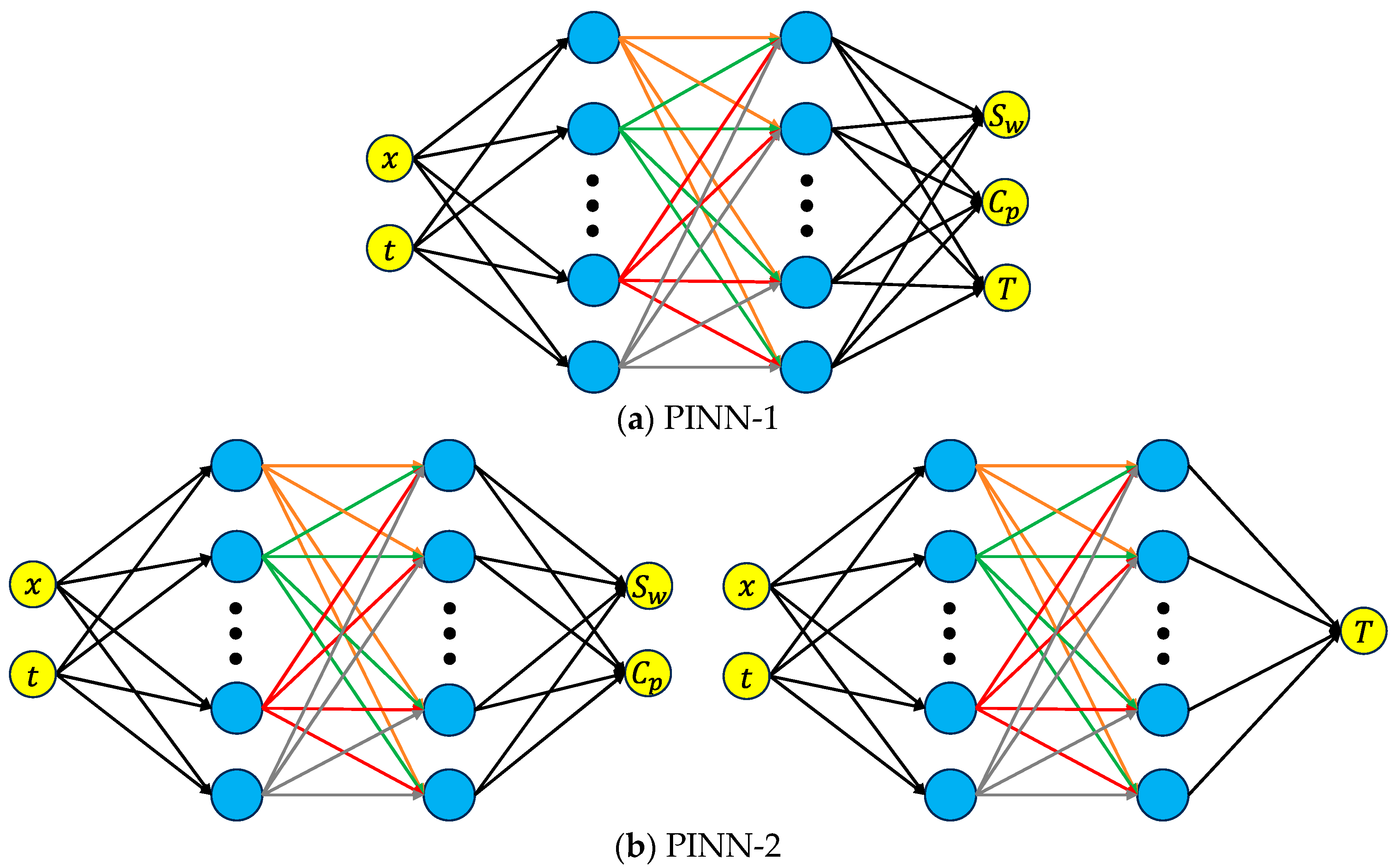
To illustrate this concept, as shown in Figure 1a, consider the approximation of water saturation (Sw), polymer concentration (Cp) and temperature (T) as an example. Drawing upon the universal approximation theorem of MLPs, PINNs construct a neural network architecture that takes spatial coordinate x and temporal coordinate t as inputs and generates Sw, Cp and T as its output, thereby approximating the PDE solution. This approach is particularly powerful because it allows the neural network to learn the underlying physical laws governing the system directly from the PDEs, rather than relying solely on data-driven methods. The network’s ability to approximate the solution is further enhanced by its capacity to incorporate physical constraints, such as boundary and initial conditions, into the training process.
Let us consider a PINN architecture comprising a fully connected MLP with L + 1 layers, including L − 1 hidden layers, where the input layer is designated as layer 0. The network’s structure can be mathematically characterized as follows: let n l represent the number of neurons in the l-th layer, l , j denote the j-th neuron in the l-th layer, x j l indicate the activation value of that neuron, and x l symbolize the vector of activation values for all neurons in the l-th layer. The network’s forward propagation can then be expressed through the following relationships:
x l = σ W l 1 x l 1 + b l ,   1 l L 1 , x L = W L 1 x L 1 + b L ,
where the output of the final layer x L serves as the approximation of the true solution, while W l 1 and b l represent the weight matrix and bias vector of the l-th layer, respectively. The function σ denotes a nonlinear activation function. Common choices for activation functions include the hyperbolic tangent (tanh), rectified linear unit (ReLU), or sinusoidal functions, depending on the nature of the problem. All trainable parameters, including weights and biases, are collectively represented by θ in subsequent discussions.
The general formulation of the MLP can be extended to:
MLP x 0 , θ = N L 1 σ N L 2 N 1 σ N 0 x 0 ,
where x 0 is the input vector, and N l x = W l 1 x + b l . The network’s architecture is designed to be flexible, allowing for the inclusion of multiple hidden layers and neurons to capture the complexity of the underlying PDEs.
The training process of PINNs involves strategically placing collocation points throughout the computational domain and along its boundaries. These collocation points serve as the “training data” for the neural network, ensuring that the network learns to satisfy the governing equations and boundary conditions. Let N i n , N I C and N B C represent the number of collocation points in the interior of the domain, for the initial conditions, and for the boundary condition, respectively. The network parameters are optimized to simultaneously satisfy the governing differential equations at interior points, initial conditions at the points and the boundary conditions at boundary points. This dual objective is achieved through the construction of a composite loss function L θ :
L θ = ω 1 L S w + ω 2 L C p + ω 3 L T + ω 4 L d a t a ,
L S w = ω 11 1 N i n j = 1 N i n S w t + q ϕ A f w x ε 2 S w x 2 2 x j , y j + ω 12 1 N I C j = 1 N I C S w S w i 2 x j , y j + ω 13 1 N B C j = 1 N B C S w 1 S o r 2 x j , y j ,
L C p = = ω 21 1 N i n j = 1 N i n S w C p t + q A ϕ f w C p x ε 2 C p x 2 2 x j , y j + ω 22 1 N I C j = 1 N I C C p 0 2 x j , y j + ω 23 1 N B C j = 1 N B C C p C p i 2 x j , y j ,
L T = = ω 31 1 N i n j = 1 N i n 1 ϕ ρ R C R T + ϕ ρ o 1 S w h o + ϕ ρ w S w h w t + q f w ρ w h w x + q 1 f w ρ o h o x 2 x j , y j + ω 32 1 N I C j = 1 N I C T T 0 2 x j , y j + ω 33 1 N B C j = 1 N B C T T i 2 x j , y j
where ω 1 , ω 2 , ω 3 , ω 4 , ω 11 , ω 12 , ω 13 , ω 21 , ω 22 , ω 23 , ω 31 , ω 32 , ω 33 are the weighting coefficients for the different loss terms. These weights are typically chosen to balance the contributions of the different loss components, ensuring that the network satisfies both the PDE and the boundary conditions with high accuracy.
In scenarios where experimental or observational data are available for water saturation, polymer concentration, or temperature at specific points, an additional error term L d a t a can be incorporated into the loss function. This term is defined as:
L d a t a = i = 1 N o b S w , i S w , i o b 2 + C p , i C p , i o b 2 + T i T i o b 2 ,
where S w , i o b , C p , i o b , and T i o b represents the observed data at the i-th point, and S w , i , C p , i , and T i denotes the PINN-predicted data at the i-th point. N o b is the total number of the observed points. However, this particular term is not considered in the current study, as the focus is on solving the PDE without relying on external data.
Through this framework, PINNs effectively transform the PDE system comprising Equations (2), (4) and (5) into an optimization problem focused on minimizing L θ through iterative updates of the neural network parameters θ . A crucial aspect of computing Equations (10)–(12) involves the implementation of Automatic Differentiation (AD). AD employs the chain rule to track the influence of each layer’s output on the preceding layer’s output, enabling direct computation of network output derivatives with respect to inputs within the computational graph. This approach allows for precise calculation of partial derivatives through explicit expressions, thereby circumventing the truncation errors inherent in traditional numerical approximation methods. The widespread adoption of AD in machine learning and optimization algorithms has significantly contributed to the advancement and implementation of PINN methodologies. Therefore, PINNs can seamlessly incorporate physical constraints, such as conservation laws or symmetry conditions, into the training process, ensuring that the learned solutions are physically consistent. This makes PINNs particularly well-suited for applications in fluid dynamics, heat transfer, and other fields governed by PDEs [43]. Beyond standard MLP-based PINNs, physics-informed Kolmogorov–Arnold networks have recently been proposed to enhance representation capability for heterogeneous porous media flow, indicating ongoing efforts to improve network expressiveness in multiphysics problems [44].
In their study on the application of PINN to single-phase flow in heterogeneous reservoirs, Lehmann et al. [45] demonstrated that a PINN architecture employing separate neural networks for pressure and velocity approximation outperforms one using a single network for both variables. Conversely, Liu et al. [34], in their investigation of PINNs for polymer flooding, observed that a PINN utilizing distinct networks for water saturation (Sw) and polymer concentration (Cp) exhibited significantly inferior performance compared to one employing a shared network for both parameters. They hypothesized that this discrepancy arises from the fact that Sw and Cp represent similar physical quantities—both being ratios of specific substances to the total mixture, with values ranging between 0 and 1. Consequently, separating their approximation into distinct networks effectively halves the parameter count for each network compared to a unified approach, potentially compromising computational performance.
Building upon Liu et al.’s [34] findings, our current work introduces temperature as an additional physical parameter. Unlike Sw and Cp, temperature represents a fundamentally different physical quantity. This leads us to investigate whether the PINN-1 architecture (illustrated in Figure 1a), which employs a shared network for T, Sw and Cp, demonstrates superior computational performance compared to the PINN-2 architecture (shown in Figure 1b), where temperature is approximated by a separate dedicated network.
In all numerical examples of this study, a unified and fixed loss-weight setting is adopted, with all loss weights set to 1, so that the PDE residual, initial conditions, and boundary conditions have equal relative importance during training. This choice is made to ensure that the comparative results for temperature normalization, network architectures, and network depth are not influenced by other hyperparameters. We acknowledge that different loss-weight selections may affect the optimization path and convergence behavior of PINNs, such as gradient imbalance and distortion of the loss landscape, as discussed in the literature (e.g., Wang et al. [35]). In future work, systematic ablation studies will be conducted to investigate the influence of loss weights on the convergence and accuracy of PAHWF PINN models, thereby improving model controllability and theoretical understanding.
In addition, In this study, the tanh activation function is adopted for the PINN due to several considerations. The PAHWF equations are highly nonlinear and convection-dominated, requiring smooth network outputs to ensure stable computation of higher-order derivatives via automatic differentiation. Compared with piecewise linear activations such as ReLU, tanh provides smoother gradients and improved stability of PDE residual optimization, and has been shown to mitigate gradient pathologies in multiphysics PINNs. Preliminary tests with ReLU and sinusoidal activations resulted in training oscillations or inferior performance for monotonic temperature and saturation fields, leading to the final selection of tanh.

3. Numerical Examples

This section presents three numerical examples designed to systematically assess the performance of the proposed polymer-assisted hot water flooding (PAHWF) PINN surrogate model from complementary perspectives. The three examples are not independent, but are organized in a progressive manner to isolate and examine key factors influencing PINN performance in multiphysics-coupled problems. Specifically, Example 1 focuses on the effect of variable scaling by comparing PINN solutions with normalized and unnormalized temperature T, aiming to identify the influence of physical magnitude disparity on training stability and accuracy. Building upon the normalized formulation validated in Example 1, Example 2 evaluates the solution performance of different PINN architectures, namely PINN-1 and PINN-2, to examine how architectural design affects convergence behavior and prediction accuracy. Based on the preferred architecture identified in Example 2, Example 3 further assesses the robustness of PINNs by varying the number of hidden layers while solving the same problem. All three examples incorporate a non-convex water-cut function to evaluate the capability of PINNs in handling complex fluid flow behavior. To enhance numerical stability and accuracy in the presence of the non-convex flux, an artificial viscosity term is introduced into the governing equations, as detailed in Equations (16)–(18) [32]. In this study, the mean squared error (MSE) at the final time t = 1.0 is selected as the error metric because nonlinear coupling effects in PAHWF accumulate over time, making the final time the most representative indicator of overall model accuracy. Moreover, the loss over the entire time domain converges to a stable level during training, ensuring that the final-time error reliably reflects the global prediction quality. This evaluation strategy is consistent with commonly adopted practices in the PINN literature. The initial and boundary conditions are specified separately for each numerical example to maintain the generality and clarity of the methodology. For each case, the corresponding Dirichlet- and Neumann-type boundary conditions associated with the governing equations are explicitly stated. In addition, to avoid biases introduced by manual weight adjustment, all loss-term weighting coefficients are uniformly set to 1 throughout this study.

3.1. Example 1

In the PAHWF governing equations, the magnitude of temperature T is much larger than that of S w and C p , which leads to gradient imbalance during PINN training. As a result, temperature-related terms dominate the PDE residuals, causing the network to prioritize minimizing temperature errors and suppressing gradient updates for S w and C p . Moreover, inconsistent gradient scales among different loss components may induce oscillatory behavior or poor convergence. To mitigate this cross-scale gradient pathology, the temperature is normalized to the same range as S w and C p [0, 1], thereby balancing the loss contributions of different physical variables and significantly improving the training stability and prediction accuracy of the PINN.
In this example, Equations (14) and (15) provide specific expressions for the relative permeability of the oil-water two-phase system as a function of water saturation.
k r w S w = 0     if   S w < S w i S w S w i 2 / 1 S o r S w i 2     if   S w i S w 1 S o r 1     if   S w > 1 S o r ,
k r o S w = 1     if   S w < S w i 1 S w S o r 2 / 1 S o r S w i 2     if   S w i S w 1 S o r 0     if   S w > 1 S o r .
Let μ w C p = 1 e 0.02 T T 0 1 + 3 C p c p , μ o C p = 50   e 0.04 T T 0 c p , S w i = S o r = 0.15 , q = 50   m 3 / day , ϕ = 0.2 , A = 25   m 2 . The relevant parameters or mathematical expressions and their values are listed in Table 1:
Substituting these parameter values into Equations (2) and (4) to obtain:
S w t + 10 f w x ε 2 S w x 2 = 0 ,   0 x 100 ,   0 t 10 ,
S w C p t + 10 f w C p x ε 2 C p x 2 = 0 ,   0 x 100 ,   0 t 10 ,
t 1896480 T + 336000 T 1 S w + 837200 T S w + 209300000 T f w x + 84000000 T 1 f w x ε 2 T x 2 = 0 ,   0 x 100 ,   0 t 10 ,
where
f w S w , C p = S w 0.15 2 S w 0.15 2 + 1 + 3 C p e 0.02 T 50 50 0.85 S w 2 .
The functional form of the water-cut function f w in Equation (19) arises from the combined derivation of the Corey relative permeability model (Equations (14) and (15)) and the temperature-dependent viscosity model (Equation (1)), rather than from any artificial assumption. Since both the water-phase viscosity μ w ( C p , T ) and the oil-phase viscosity μ o ( T ) explicitly depend on temperature, the influence of temperature T enters the water-cut function through the viscosity ratio μ w / μ o , thereby directly affecting the magnitude and shape of f w .
ε 2 S w x 2 , ε 2 C p x 2 and, ε 2 T x 2 is the artificial viscosity terms, ε is coefficient of artificial viscosity. We selected ε = 10 4 to optimize the trade-off between model stability and solution accuracy. For hyperbolic equations arising from non-convex water-cut functions, PINNs often struggle to directly capture sharp shock-like fronts and are prone to producing nonphysical oscillations. Previous studies, including the PINN-based convection equation analysis for polymer flooding by Liu et al. [27], have demonstrated that introducing a small artificial viscosity term into the governing equations can effectively improve the trainability and stability of PINN solutions. The artificial viscosity is typically chosen within the range ε [ 10 6 , 10 4 ] . Following these established practices, this study adopts ε = 10 4 , which provides sufficient smoothing to ensure stable training while avoiding significant distortion of the physical front location and shape. Numerical tests further indicate that when ε < 10 4 , PINN training becomes unstable, whereas larger values of ε lead to mild over-smoothing of the front. Therefore, ε = 10 4 represents a reasonable compromise between numerical stability and physical fidelity.
Let x = 100 X , t = 10 τ , and perform a coordinate transformation to obtain:
S w τ + f w X ε 2 S w x 2 = 0 ,   0 X 1 ,   0 τ 1 ,
S w C p τ + f w C p X ε 2 C p x 2 = 0 ,   0 X 1 ,   0 τ 1 ,
τ 189648 T + 33600 T 1 S w + 83720 T S w + 83720 T f w X + 33600 T 1 f w X ε 2 T x 2 = 0 ,   0 X 1 ,   0 τ 1 .
Given the initial conditions and boundary conditions as follows:
S w X , τ = 0 = 0.20 ,   C p X , τ = 0 = 0 ,   T X , τ = 0 = 50 ,
and the boundary conditions:
S w X = 0 , T = 0.80 ,   C p X = 0 , T = 0.6 ,   T X = 0 , τ = 100 .
It should be noted that Equations (20)–(22) differ significantly in their order of magnitude due to the involvement of quantities of different physical scales. This disparity in magnitudes can pose challenges when solving these equations using PINNs, as the varying scales of the quantities involved might influence the optimization process. So, in this example, to investigate the effect of scaling on the PINN-based solution, it is proposed to compare two different models: one where the temperature T is normalized and another where T remains unnormalized. This comparison will help explore the impact of unifying the physical scales on the performance and accuracy of the PINN when solving the given PDE system.
Specifically, we normalize the temperature T from a range of 50 , 100 to a range of 0 , 1 :
T ˜ = T 50 100 50 = T 50 50 ,
The value range of the normalized temperature T ˜ is 0 , 1 , which is consistent with the range of S w and C p to be solved. This to some extent ensures the unbiasedness of the loss function on multiple predictor variables and performs fair and consistent backpropagation based on the loss value. At the same time, the water content function Equation (19) and the heat transfer equation, Equation (22), which originally involved temperature, will change accordingly:
f w S w , C p = S w 0.15 2 S w 0.15 2 + 1 + 3 C p e T ˜ 50 e 2 T ˜ 0.85 S w 2 ,
τ 189648 T ˜ + 1 + 33600 T ˜ + 1 1 S w + 83720 T ˜ + 1 S w + 83720 T ˜ + 1 f w X + 33600 T ˜ + 1 1 f w X = 0 .
To ensure a fair comparison, we employ a single PINN to solve two distinct sets of governing equations. Specifically, the first set comprises Equations (16)–(19), representing the non-normalized temperature, T, control equations. The second set consists of Equations (16), (17), (26) and (27), representing the control equations with temperature, T, normalized.
Table 2 provides the key parameters for the PINN model used in this example. Latin Hypercube Sampling was performed on the time and spatial domains ( t 0 , 1 , x 0 , 1 ), utilizing 20,000 random sample points. Boundary conditions were enforced at the specified locations using 2000 sample points, while initial conditions were similarly applied at designated points with another 2000 sample points. The ADAM optimizer was used throughout the training process to minimize the loss function, with a total of 15,000 iterations and a learning rate set to 10−3.
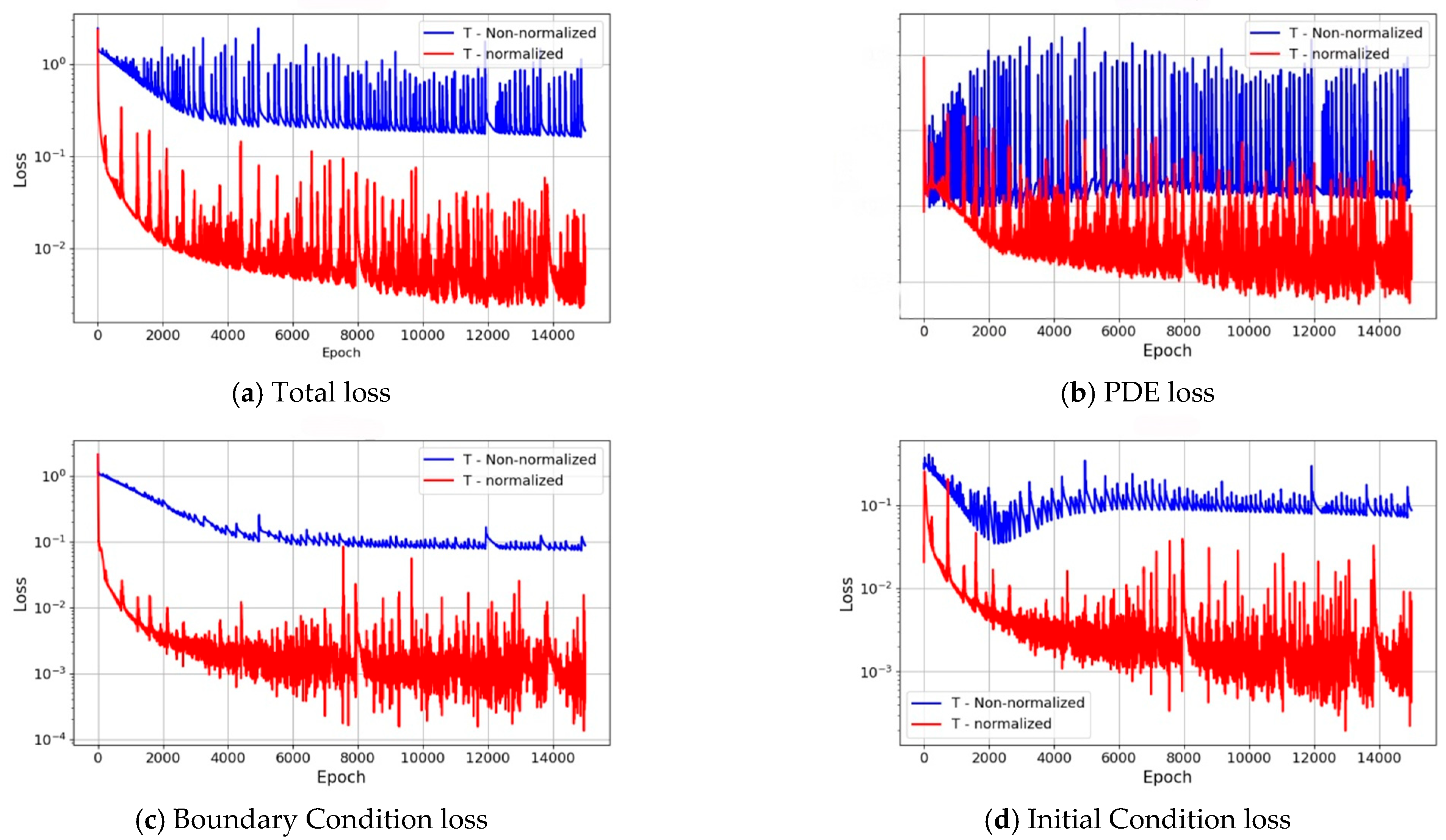
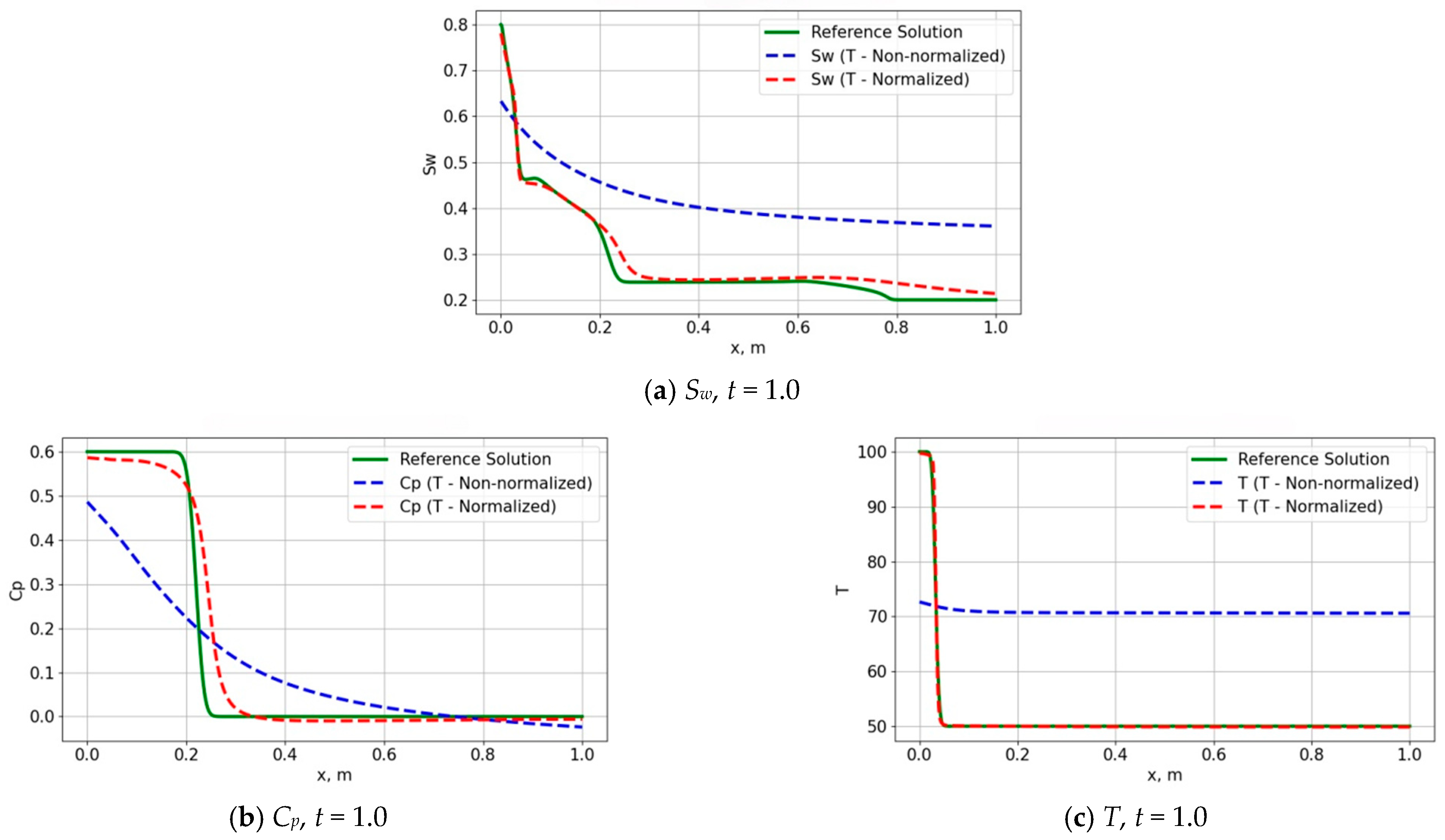
Figure 2 presents a comparative analysis of the total loss function and its constituent elements (comprising PDE loss, Boundary Condition (BC) loss, and Initial Condition (IC) loss) for both models across the training iterations. In Figure 2, the blue curve represents the loss function without normalization, while the red curve represents the normalized loss function. Figure 3 provides a comparison of the predicted water saturation Sw, polymer concentration Cp, and temperature T distributions generated by the two models at t = 1.0, juxtaposed with the reference solution. In Figure 3, the green solid line represents the reference numerical solution. In the three panels, the blue dashed lines denote the predicted water saturation, polymer concentration, and temperature obtained from the PINN with non-normalized temperature, while the green dashed lines represent the corresponding predictions from the PINN with normalized temperature. All reference solutions in this study are obtained using conventional numerical methods. Specifically, the governing equations are discretized using a first-order upwind finite difference scheme and solved with an explicit time-marching method. The spatial domain is uniformly discretized with a grid spacing of and the temporal step size is chosen as with numerical stability controlled according to the CFL condition. The resulting finite difference solutions are treated as reference solutions for comparison with the PINN predictions and are consistently used across all numerical examples.
A comparative analysis of the training loss evolution for identical PINNs, with and without normalization, reveals significant disparities across total loss, PDE loss, boundary condition loss, and initial condition loss. The normalized temperature model demonstrates accelerated convergence and reduced fluctuation in loss values, indicating that normalization effectively enhances the stability and efficiency of the PINN training process. Furthermore, Figure 3 compares the distributions of Sw, Cp, and T at t = 1.0, clearly illustrating that the PINN results with normalized T (red dashed line) closely align with the reference solution (green solid line), exhibiting only minor distortions. Conversely, the non-normalized results (blue dashed line) fail to accurately capture the spatiotemporal evolution of the three variables, leading to significant deviations in the predicted outcomes. Notably, the non-normalized model exhibits substantial distortion in the prediction of the temperature field distribution, failing to reflect the actual physical process. Table 3 further presents the impact of normalization on the mean squared error (MSE) values of variable predictions. Comparing the error levels, we observe that the MSE with normalization is significantly lower than without normalization, further validating the advantages of normalization in improving model accuracy. In conclusion, the introduction of normalization effectively balances the weights of the loss functions for each predicted variable, enabling the neural network to obtain accurate backpropagation gradients. For PINN models with multiple prediction targets, employing normalized temperature T not only significantly reduces the fluctuation of the loss function during the model convergence process and shortens the convergence time but also enhances prediction accuracy, thereby improving the overall accuracy of the prediction results. This conclusion is of significant importance for subsequent research on PINN modeling in complex physical problems.

3.2. Example 2

Following the demonstration of the significant benefits of normalization, we will conduct a comprehensive evaluation and comparison of the performance of PINN-1 and PINN-2 in solving the normalized mathematical model in Example 2. Table 4 presents the relevant parameters of PINN-1 and PINN-2 constructed in this example, where the PINN-1 architecture is consistent with that used in Example 1. To ensure that the performance comparison is not influenced by factors such as the number of network parameters, we have adopted similar network configurations and unified several key training parameters, including sampling strategy, sample quantity, optimizer type, iteration steps, and learning rate.
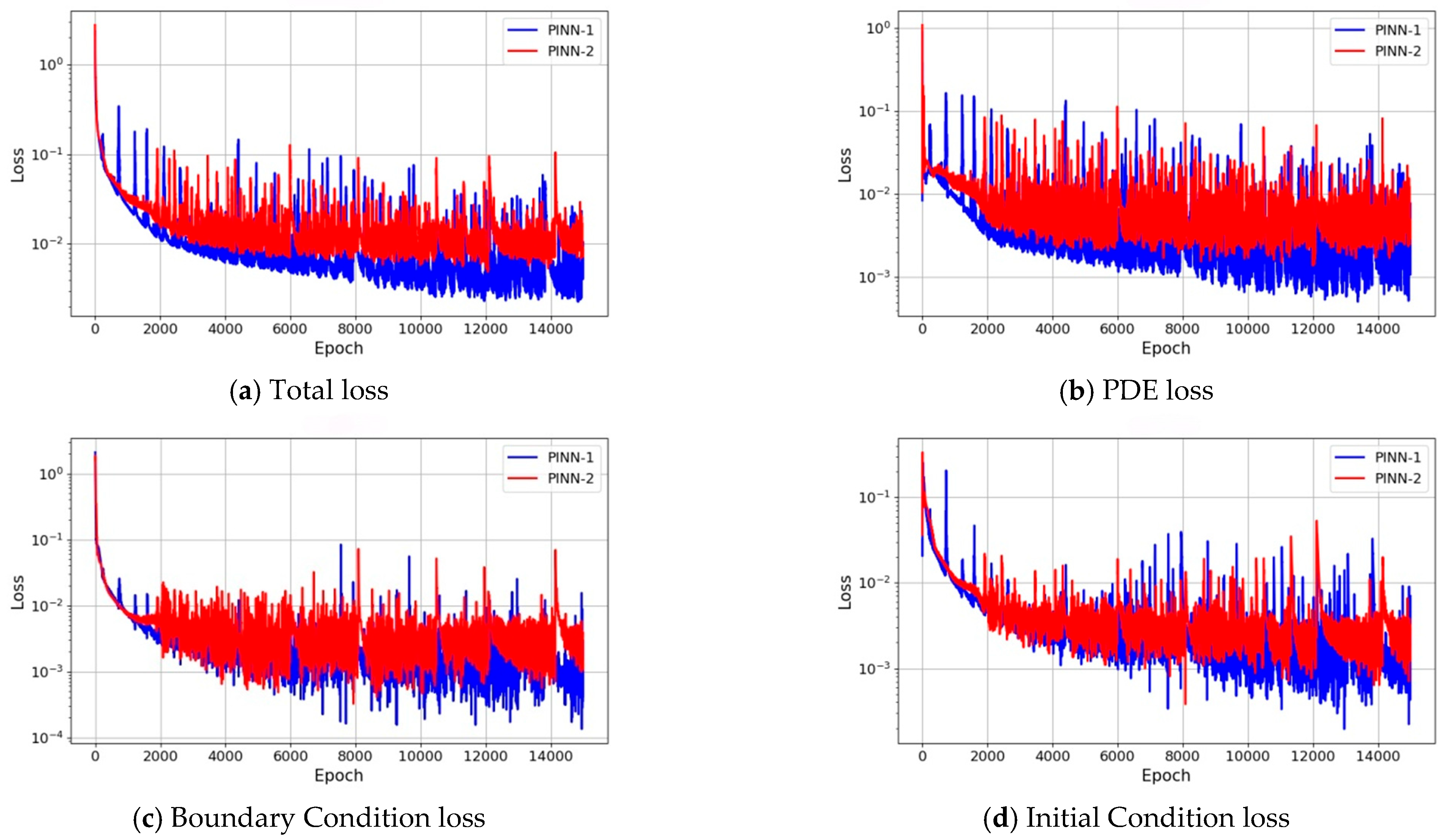
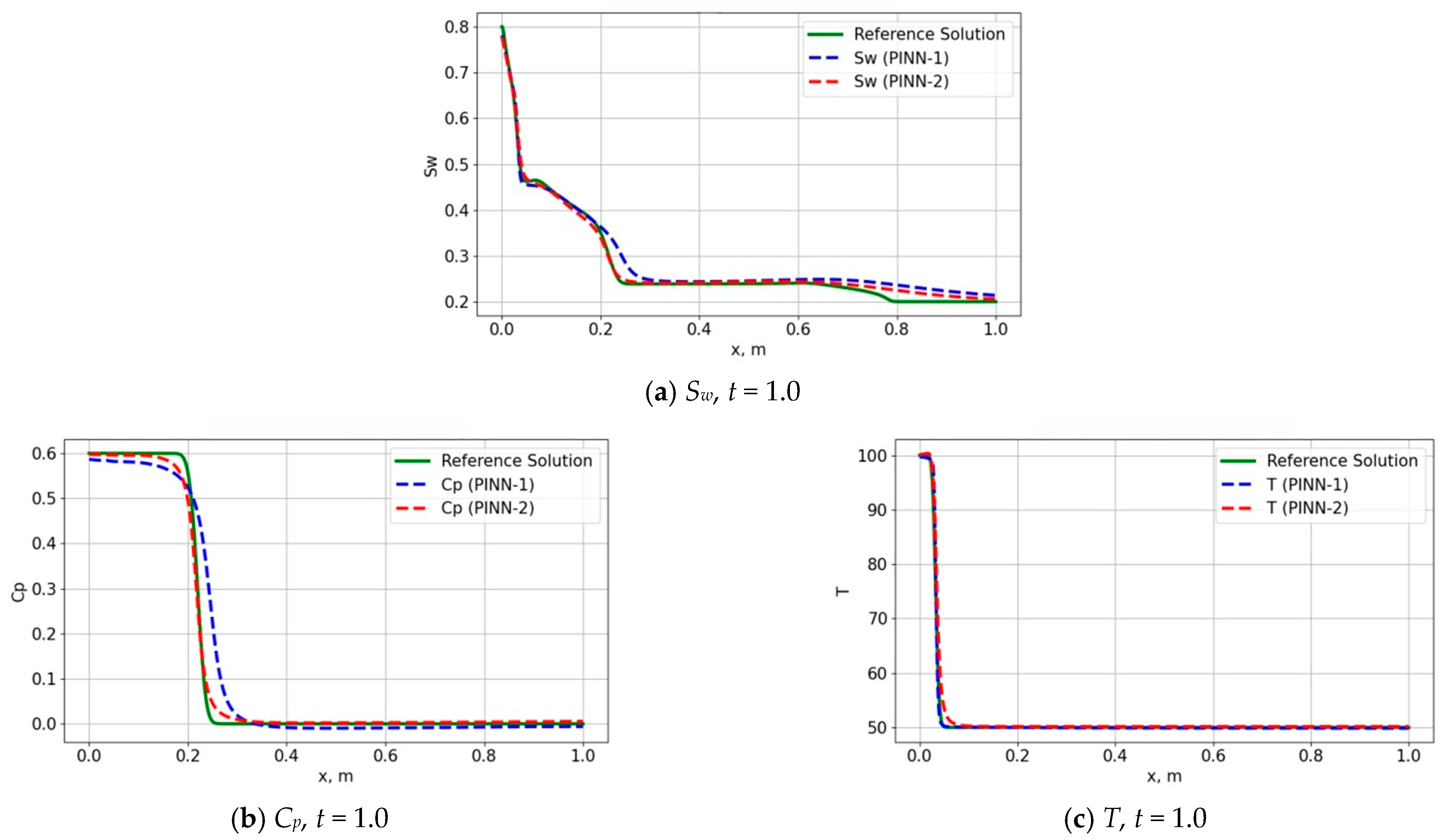
Figure 4 presents a comparative analysis of the total loss function and its constituent components over the entire training process, in which the blue curve represents the loss function of PINN-1, while the red curve represents the loss function of PINN-2. Figure 5 compares the predicted distributions of Sw, Cp, and T at t = 1.0 for both models, benchmarked against the reference solution. In Figure 5, the green solid line represents the reference numerical solution. In the three panels, the blue dashed lines denote the water saturation, polymer concentration, and temperature predicted by PINN-1, while the green dashed lines represent the corresponding predictions obtained from PINN-2.
As illustrated in Figure 4, both PINN-1 and PINN-2 exhibited comparable total loss, PDE loss, boundary condition loss, and initial condition loss during training. However, PINN-2 demonstrated significantly reduced loss fluctuations compared to PINN-1, indicating superior training stability in addressing this class of problems, which leads to more reliable solution outcomes. A comparison of the solutions from PINN-1 and PINN-2 with the reference solution in Figure 5 reveals that, at t = 1.0, PINN-2 outperforms PINN-1 in predicting Sw and Cp, with its predictions accurately capturing the evolution of the reference solution. Regarding temperature prediction, both models exhibited excellent accuracy, with only minor discrepancies. Despite a slight underperformance in temperature T prediction accuracy, PINN-2 still achieved satisfactory predictive results overall, demonstrating its enhanced adaptability and predictive capabilities in handling multi-variable problems. The MSE comparison in Table 5 further corroborates this, with PINN-2 achieving lower error values for both Sw and Cp, indicating its greater efficacy in capturing and approximating the true solution in complex physical modeling, thereby improving the accuracy and reliability of the computational results. Consequently, while both architectures effectively solve the problem, PINN-2 demonstrates a slight advantage over PINN-1 in computational stability, accuracy, and the ability to handle multi-variable problems, further validating its reliability in high-precision solutions and complex physical process modeling.

3.3. Example 3

This example further evaluates the performance of PINN-2 architectures, varying the number of hidden layers, in solving the normalized mathematical model. This investigation aims to elucidate the impact of hidden layer count on the computational accuracy and convergence rate of the PINN model. Specifically, the PINN-2 model with eight hidden layers mirrors the architecture employed in Example 2, while the PINN-2 model with ten hidden layers incorporates an additional two hidden layers. The sampling strategy, sample quantity, optimizer type, iteration steps, and learning rate remain consistent with the configurations used in Examples 1 and 2. Table 6 provides a summary of the parameters for the PINN-2 (8-layer) and PINN-2 (10-layer) models utilized in this example.
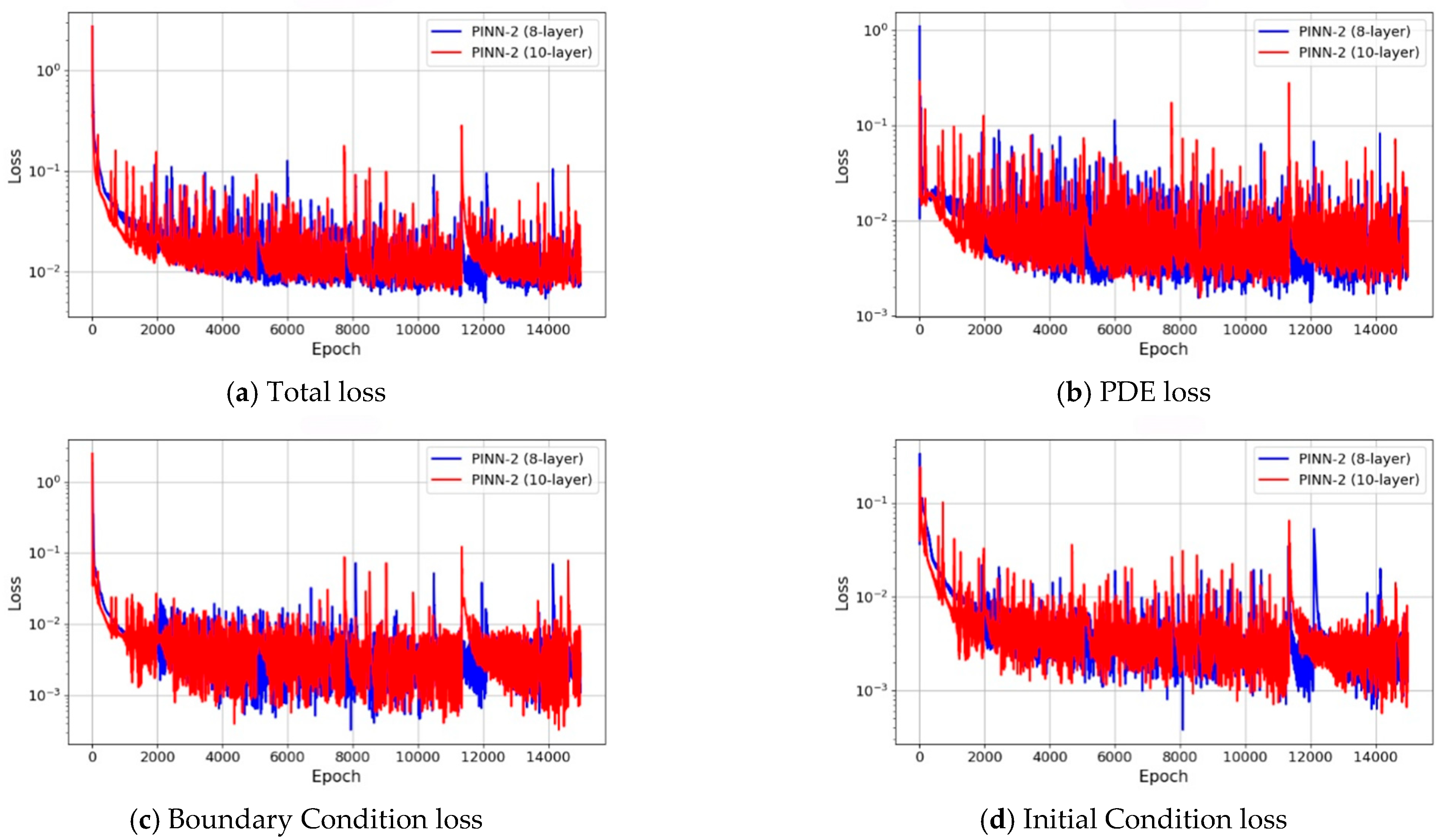
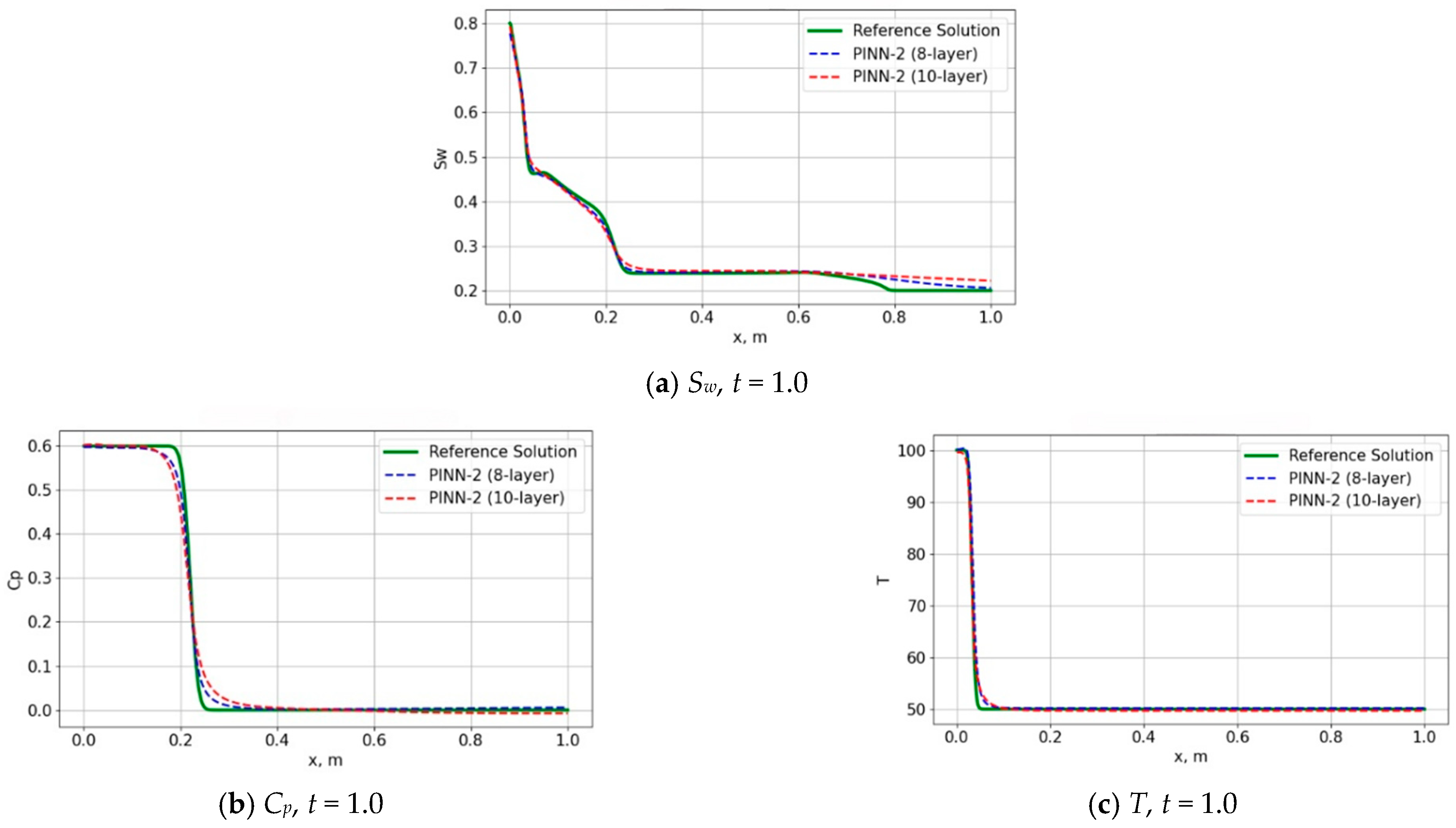
Figure 6 presents a comparison of the total loss function and its individual components for both models. Figure 7 compares the predicted distributions of water saturation, polymer concentration, and temperature at t = 1.0 for both models with the reference solution.
The comparative analysis of the loss functions, as depicted in Figure 6, reveals that the 10-layer PINN-2 and the 8-layer PINN-2 exhibit nearly identical convergence rates. In this figure, the blue curve represents the loss function of the 8-layer PINN-2, while the red curve represents the loss function of the 10-layer PINN-2. This observation suggests that the network architectures, despite variations in the number of hidden layers, demonstrate similar stability and convergence characteristics during training, thereby indicating the model’s robustness when addressing the same problem. Furthermore, the distributions of Sw, Cp, and T at t = 1.0, as presented in Figure 7, demonstrate that both the 10-layer PINN-2 and the 8-layer PINN-2 achieve satisfactory predictive performance. In Figure 7, the green solid line represents the reference numerical solution. In the three panels, the blue dashed lines denote the water saturation, polymer concentration, and temperature predicted by the 8-layer PINN-2, while the green dashed lines represent the corresponding predictions obtained from the 10-layer PINN-2. Although the 10-layer PINN-2’s predictions are slightly less accurate than those of the 8-layer PINN-2, we posit that as network depth increases, issues such as vanishing or exploding gradients become more pronounced, often impeding effective learning in the early layers. Additionally, the more complex loss landscape associated with deeper models complicates the optimization process, especially when balancing the dual objectives of fitting data and enforcing physical constraints imposed by the governing equations. Despite these challenges, the capacity of PINNs to capture complex nonlinear relationships across varying depths still highlights their inherent robustness. The MSE values for various variables, as detailed in Table 7, are closely aligned for PINN-2 models with different layer counts. This indicates that PINNs with varying depths possess similar accuracy and stability when solving the same physical problem. Consequently, the alteration in network depth does not significantly impact the model’s ability to solve this problem, further validating the PINN model’s robustness across different architectures.

4. Conclusions and Future Work

In this study on applying Physics-Informed Neural Networks (PINNs) to Polymer-assisted hot water flooding (PAHWF) simulations, several significant findings were obtained. First, normalizing the temperature in PINN models effectively balances the weights of the loss functions for each predicted variable. This not only reduces the fluctuation of the loss function during the convergence process and shortens the convergence time but also remarkably enhances the prediction accuracy, which is of great importance for PINN applications in complex physical problems. Second, when comparing the PINN-1 and PINN-2 architectures, PINN-2 shows a slight edge in computational stability, accuracy, and the ability to handle multi-variable problems. Although both can solve the problem effectively, PINN-2 has less loss fluctuations during training and provides more accurate predictions for water saturation and polymer concentration, with satisfactory temperature prediction results as well. Third, varying the number of hidden layers in the PINN-2 architecture does not significantly affect the model’s problem-solving ability. The 8-layer and 10-layer PINN-2 models have similar convergence rates and predictive performance, indicating the robustness of PINNs across different architectures when dealing with the same physical problem, despite potential issues like vanishing or exploding gradients in deeper networks. PINNs are often affected by several typical computational challenges when solving complex PDEs, including vanishing or exploding gradients, training instability caused by stiff terms, early-stage oscillations of optimizers such as ADAM, and the widely reported failure of L-BFGS. In the present one-dimensional PAHWF model, the convection-dominated nature of the governing equations and nonlinear coupling terms lead to severe gradient-scale imbalance. This issue is partially alleviated through temperature normalization and structured network design, and the ADAM optimizer is preferentially adopted to achieve more stable convergence. In future work, when extending the framework to two- and three-dimensional PAHWF models, we will systematically investigate stiffness, gradient degradation in deep networks, and the failure mechanisms of L-BFGS in multiphysics coupling problems, and explore more effective mitigation strategies such as staged training, gradient clipping, and adaptive loss balancing to further improve the trainability and robustness of PINNs. Overall, PINNs have great potential in PAHWF simulations. They can efficiently manage the high-dimensional parameter space, integrate physical laws and observational data, and significantly cut down computational costs compared to traditional numerical methods. Thus, they are suitable for real-time decision-making and optimization in reservoir management, providing a powerful means to revolutionize the modeling and optimization of this enhanced oil recovery technique. It should be noted that although one-dimensional PAHWF problems can be solved efficiently at very low cost using conventional numerical methods, the purpose of this study is not to position PINNs as a replacement for traditional solvers in 1D forward problems. Instead, the 1D model serves as a reliable benchmark for systematically analyzing PINN behavior in strongly coupled, multi-scale physical systems, including gradient stability, architectural effects, and normalization strategies. While we acknowledge that PINN training is more computationally expensive than classical methods in 1D cases, the goal of this work is to establish a methodological foundation for future extensions to high-dimensional, multiphysics, and inverse reservoir problems, where PINNs offer greater potential advantages. Although this study is based on a one-dimensional PAHWF model, its primary objective is to provide a controlled testbed for systematically analyzing the effects of temperature normalization, PINN architecture, and network depth on solution performance. We acknowledge that a one-dimensional geometry cannot fully capture key reservoir processes such as lateral flow redistribution, gravity-driven segregation, the competition between thermal convection and diffusion, and multidimensional heterogeneity. Therefore, for more complex physical scenarios including two-and three-dimensional thermo-chemical-flow coupling, interwell interference, and multidimensional front evolution, we plan to develop high-dimensional PINN models in future work to further validate the applicability of the conclusions under realistic reservoir conditions. As a foundational study, the framework and methodology proposed herein are readily extendable to multidimensional systems.

Author Contributions

Conceptualization, methodology, validation, investigation, data curation, writing—original draft preparation, writing—review and editing, S.C.; validation, visualization, supervision, X.O.; Conceptualization, methodology, investigation, supervision, project administration, X.R. All authors have read and agreed to the published version of the manuscript.

Funding

This research was funded by the General Program of the National Natural Science Foundation of China (Grant No. 52574028) and the National Science and Technology Major Project (Grant No. 2025ZD1401106).

Data Availability Statement

The data supporting the findings of this study are available from the corresponding author upon reasonable request.

Acknowledgments

Authors thank the open fund of Hubei Key Laboratory of Oil and Gas Drilling and Production Engineering (Yangtze University) for its support in analysis and testing.

Conflicts of Interest

The authors declare no conflicts of interest to report regarding the present study.

References

  1. Lake, L.W.; Johns, R.T.; Rossen, W.R.; Gary, A.P. Fundamentals of Enhanced Oil Recovery; Society of Petroleum Engineers: Richardson, TX, USA, 2014. [Google Scholar]
  2. Delshad, M.; Pope, G.A.; Sepehrnoori, K. A compositional simulator for modeling surfactant enhanced aquifer remediation, 1. Formulation. J. Contam. Hydrol. 1996, 23, 303–327. [Google Scholar] [CrossRef] [Scilit]
  3. Chen, Z.; Huan, G.; Ma, Y. Computational Methods for Multiphase Flows in Porous Media; Society for Industrial and Applied Mathematics: Philadelphia, PA, USA, 2006. [Google Scholar]
  4. Aziz, K.; Settari, A. Petroleum Reservoir Simulation; Applied Science Publishers: London, UK, 1979. [Google Scholar]
  5. Rao, X.; Guo, S.; He, X.; Kwak, H.; Hoteit, H. A first streamline-based simulation method within the projection-based embedded discrete fracture model (pEDFM). Comput. Geotech. 2025, 185, 107357. [Google Scholar] [CrossRef] [Scilit]
  6. Rao, X.; He, X.; Du, K.; Kwak, H.; Yousef, A.; Hoteit, H. A novel projection-based embedded discrete fracture model (pEDFM) for anisotropic two-phase flow simulation using hybrid of two-point flux approximation and mimetic finite difference (TPFA-MFD) methods. J. Comput. Phys. 2024, 499, 112736. [Google Scholar] [CrossRef] [Scilit]
  7. Rao, X.; Zhao, H.; Liu, Y. A meshless numerical modeling method for fractured reservoirs based on extended finite volume method. SPE J. 2022, 27, 3525–3564. [Google Scholar] [CrossRef] [Scilit]
  8. Lawal, Z.K.; Yassin, H.; Lai, D.T.C.; Che Idris, A. Physics-informed neural network (PINN) evolution and beyond: A systematic literature review and bibliometric analysis. Big Data Cogn. Comput. 2022, 6, 140. [Google Scholar] [CrossRef] [Scilit]
  9. Karniadakis, G.E.; Kevrekidis, I.G.; Lu, L.; Perdikaris, P.; Wang, S.; Yang, L. Physics-informed machine learning. Nat. Rev. Phys. 2021, 3, 422–440. [Google Scholar] [CrossRef] [Scilit]
  10. Raissi, M.; Perdikaris, P.; Karniadakis, G.E. Physics-informed neural networks: A deep learning framework for solving forward and inverse problems involving nonlinear partial differential equations. J. Comput. Phys. 2019, 378, 686–707. [Google Scholar] [CrossRef] [Scilit]
  11. Raissi, M.; Yazdani, A.; Karniadakis, G.E. Hidden fluid mechanics: Learning velocity and pressure fields from flow visualizations. Science 2020, 367, 1026–1030. [Google Scholar] [CrossRef] [Scilit]
  12. Cai, S.; Mao, Z.; Wang, Z.; Perdikaris, P.; Karniadakis, G.E. Physics-informed neural networks (PINNs) for heat transfer problems. J. Heat Transf. 2021, 143, 060801. [Google Scholar] [CrossRef] [Scilit]
  13. Zhang, Y.; Wang, H.; Chen, W. Physics-informed neural networks for reservoir simulation: A case study on polymer flooding. J. Pet. Sci. Eng. 2022, 208, 109456. [Google Scholar]
  14. He, Q.; Barajas-Solano, D.; Tartakovsky, G.; Tartakovsky, A.M. Physics-informed neural networks for multiphysics data assimilation with application to subsurface transport. Adv. Water Resour. 2020, 141, 103610. [Google Scholar] [CrossRef] [Scilit]
  15. Wang, S.; Teng, Y.; Perdikaris, P. Understanding and mitigating gradient pathologies in physics-informed neural networks. SIAM J. Sci. Comput. 2021, 43, A3055–A3081. [Google Scholar] [CrossRef] [Scilit]
  16. Mao, Z.; Jagtap, A.D.; Karniadakis, G.E. Physics-informed neural networks for high-speed flows. Comput. Methods Appl. Mech. Eng. 2020, 360, 112789. [Google Scholar] [CrossRef] [Scilit]
  17. Bararnia, H.; Esmaeilpour, M. On the application of physics informed neural networks (PINN) to solve boundary layer thermal-fluid problems. Int. Commun. Heat Mass Transf. 2022, 132, 105890. [Google Scholar] [CrossRef] [Scilit]
  18. Ke, C.Y.; Sun, W.J.; Li, Y.B.; Hui, J.F.; Lu, G.M.; Zheng, X.Y.; Zhang, Q.-Z.; Zhang, X.L. Polymer-assisted microbial-enhanced oil recovery. Energy Fuels 2018, 32, 5885–5892. [Google Scholar] [CrossRef] [Scilit]
  19. Chen, X.; Li, Y.; Sun, X.; Liu, Z.; Liu, J.; Liu, S. Investigation of polymer-assisted CO2 flooding to enhance oil recovery in low-permeability reservoirs. Polymers 2023, 15, 3886. [Google Scholar] [CrossRef] [Scilit]
  20. Sun, L.; Gao, H.; Pan, S.; Wang, J.-X. Surrogate modeling for fluid flows based on physics-constrained deep learning without simulation data. Comput. Methods Appl. Mech. Eng. 2020, 361, 112732. [Google Scholar] [CrossRef] [Scilit]
  21. Tartakovsky, A.M.; Marrero, C.O.; Perdikaris, P.; Tartakovsky, G.D.; Barajas-Solano, D. Physics-informed deep neural networks for learning parameters and constitutive relationships in subsurface flow problems. Water Resour. Res. 2020, 56, e2019WR026731. [Google Scholar] [CrossRef] [Scilit]
  22. Zhu, Y.; Zabaras, N.; Koutsourelakis, P.S.; Perdikaris, P. Physics-constrained deep learning for high-dimensional surrogate modeling and uncertainty quantification without labeled data. J. Comput. Phys. 2019, 394, 56–81. [Google Scholar] [CrossRef] [Scilit]
  23. Chiu, P.H.; Wong, J.C.; Ooi, C.; Dao, M.H.; Ong, Y.S. CAN-PINN: A fast physics-informed neural network based on coupled-automatic–numerical differentiation method. Comput. Methods Appl. Mech. Eng. 2022, 395, 114909. [Google Scholar] [CrossRef] [Scilit]
  24. Rao, X.; Luo, C.; He, X.; Hyung, K. An Efficient Quantum Neural Network Model for Prediction of Carbon Dioxide CO2 Sequestration in Saline Aquifers. In Proceedings of the Abu Dhabi International Petroleum Exhibition and Conference, Abu Dhabi, United Arab Emirates, 4–7 November 2024; SPE: Abu Dhabi, United Arab Emirates, 2024; p. D021S061R005. [Google Scholar] [CrossRef] [Scilit]
  25. Zhang, D.; Guo, L.; Karniadakis, G.E. Learning in modal space: Solving time-dependent stochastic PDEs using physics-informed neural networks. SIAM J. Sci. Comput. 2020, 42, A639–A665. [Google Scholar] [CrossRef] [Scilit]
  26. Rao, X.; Liu, Y.; Fu, Q.; He, X.; Kwak, H.; Zhao, H.; Hoteit, H. Boundary-Integral Type Neural Network (BINN) for Flow Problems in Anisotropic Reservoirs. In Proceedings of the SPE Middle East Oil and Gas Show and Conference, Abu Dhabi, United Arab Emirates, 16–18 September 2025; SPE: Abu Dhabi, United Arab Emirates, 2025; p. D021S048R001. [Google Scholar] [CrossRef] [Scilit]
  27. Liu, Y.; Rao, X.; He, X.; Fu, Q.; Hoteit, H. Boundary-Integral Type Neural Network (BINN) for Flow Problems in Homogeneous Reservoirs. In Proceedings of the SPE Middle East Oil and Gas Show and Conference, Manama, Bahrain, 16–18 September 2025; SPE: Abu Dhabi, United Arab Emirates, 2025; p. D011S024R002. [Google Scholar] [CrossRef] [Scilit]
  28. Rao, X. The first application of quantum computing algorithm in streamline-based simulation of water-flooding reservoirs. In Proceedings of the Abu Dhabi International Petroleum Exhibition and Conference, Abu Dhabi, United Arab Emirates, 4–7 November 2024; SPE: Abu Dhabi, United Arab Emirates, 2024; p. D011S003R006. [Google Scholar] [CrossRef] [Scilit]
  29. Meng, Z.; Qian, Q.; Xu, M.; Yu, B.; Yıldız, A.R.; Mirjalili, S. PINN-FORM: A new physics-informed neural network for reliability analysis with partial differential equation. Comput. Methods Appl. Mech. Eng. 2023, 414, 116172. [Google Scholar] [CrossRef] [Scilit]
  30. Yuan, L.; Ni, Y.Q.; Deng, X.Y.; Hao, S. A-PINN: Auxiliary physics informed neural networks for forward and inverse problems of nonlinear integro-differential equations. J. Comput. Phys. 2022, 462, 111260. [Google Scholar] [CrossRef] [Scilit]
  31. Ji, W.; Qiu, W.; Shi, Z.; Pan, S.; Deng, S. Stiff-pinn: Physics-informed neural network for stiff chemical kinetics. J. Phys. Chem. A 2021, 125, 8098–8106. [Google Scholar] [CrossRef] [Scilit]
  32. Fuks, O.; Tchelepi, H.A. Limitations of physics informed machine learning for nonlinear two-phase transport in porous media. J. Mach. Learn. Model. Comput. 2020, 1, 19–37. [Google Scholar] [CrossRef] [Scilit]
  33. Tartakovsky, A.M.; Marrero, C.O.; Perdikaris, P.; Tartakovsky, G.D.; Barajas-Solano, D. Physics-informed neural networks for parameter estimation and uncertainty quantification in subsurface flow problems. Water Resour. Res. 2021, 57, e2020WR029234. [Google Scholar]
  34. Liu, B.; Wei, J.; Kang, L.; Liu, Y.; Rao, X. Physics-Informed Neural Network (PINNs) for Convection Equations in Polymer flooding reservoirs. Phys. Fluids 2025, 37, 036622. [Google Scholar] [CrossRef] [Scilit]
  35. Wang, S.; Teng, Y.; Perdikaris, P. Physics-informed neural networks for reservoir simulation: A comprehensive review and future directions. J. Pet. Sci. Eng. 2022, 210, 110032. [Google Scholar]
  36. Haider, J.; Aeschbacher, P.; Bose, M. Toward an Analytic Framework for Active Living; Pennsylvania State University: University Park, PA, USA, 2011. [Google Scholar]
  37. Wandel, N.; Weinmann, M.; Neidlin, M.; Klein, R. Spline-pinn: Approaching pdes without data using fast, physics-informed hermite-spline cnns. In Proceedings of the AAAI Conference on Artificial Intelligence, Virtual, 22 February–1 March 2022; Volume 36, pp. 8529–8538. [Google Scholar] [CrossRef] [Scilit]
  38. Wang, Y.; Han, X.; Chang, C.Y.; Zha, D.; Braga-Neto, U.; Hu, X. Auto-PINN: Understanding and optimizing physics-informed neural architecture. arXiv 2022, arXiv:2205.13748. [Google Scholar] [CrossRef] [Scilit]
  39. Kumar Thirugnanasambandam, M.; Pinto, J.; Moskovkina, E.; Costa, R.S.; Oliveira, R. A Physics-Informed Neural Network (PINN) framework for generic bioreactor modelling. Comput. Chem. Eng. 2025, 203, 109354. [Google Scholar] [CrossRef] [Scilit]
  40. Ramos, D.J.; Cunha, B.Z.; Daniel, G.B. Evaluation of physics-informed neural networks (PINN) in the solution of the Reynolds equation. J. Braz. Soc. Mech. Sci. Eng. 2023, 45, 568. [Google Scholar] [CrossRef] [Scilit]
  41. Pu, J.; Li, J.; Chen, Y. Solving localized wave solutions of the derivative nonlinear Schrödinger equation using an improved PINN method. Nonlinear Dyn. 2021, 105, 1723–1739. [Google Scholar] [CrossRef] [Scilit]
  42. Xia, Y.; Meng, Y. Physics-informed neural network (pinn) for solving frictional contact temperature and inversely evaluating relevant input parameters. Lubricants 2024, 12, 62. [Google Scholar] [CrossRef] [Scilit]
  43. Hu, H.; Qi, L.; Chao, X. Physics-informed Neural Networks (PINN) for computational solid mechanics: Numerical frameworks and applications. Thin-Walled Struct. 2024, 205, 112495. [Google Scholar] [CrossRef] [Scilit]
  44. Lau, G.K.R.; Hemachandra, A.; Ng, S.K.; Low, B.K.H. PINNACLE: PINN Adaptive ColLocation and Experimental points selection. arXiv 2024, arXiv:2404.07662. [Google Scholar] [CrossRef] [Scilit]
  45. Lehmann, F.; Fahs, M.; Alhubail, A.; Hoteit, H. A mixed pressure-velocity formulation to model flow in heterogeneous porous media with physics-informed neural networks. Adv. Water Resour. 2023, 181, 104564. [Google Scholar] [CrossRef] [Scilit]
Figure 1. The schematic diagram of the network architectures for the two types of PINN models used in this study.
Processes 14 00197 g001
Figure 2. Comparison of the Loss function and its sub-terms (including PDE loss, loss of boundary condition, and loss of initial condition) for Normalized and Non-normalized Temperature in PINN.
Processes 14 00197 g002
Figure 3. Comparison of Water Saturation, Concentration, and Temperature Solutions at t = 1.0 for Normalized and Non-normalized Temperature in PINN.
Processes 14 00197 g003
Figure 4. Comparison of Loss function and its sub-terms (including PDE loss, loss of boundary condition, and loss of initial condition) for PINN-1 and PINN-2.
Processes 14 00197 g004
Figure 5. Comparison of Water Saturation, Concentration, and Temperature Solutions at t = 1.0 for PINN-1 and PINN-2.
Processes 14 00197 g005
Figure 6. Comparison of the Loss function and its sub-terms (including PDE loss, loss of boundary condition, and loss of initial condition) for PINN-2 (8-layer) and PINN-2 (10-layer).
Processes 14 00197 g006
Figure 7. Comparison of Water Saturation, Concentration, and Temperature Solutions at t = 1.0 for PINN-2 (8 layers) and PINN-2 (10 layers).
Processes 14 00197 g007
Table 1. The parameters or mathematical expressions and their values involved in Equations (16)–(18).
Parameters or Mathematical ExpressionsValue
q 50   m 3 / day
ϕ 0.2
ρ R 2700   kg / m 3
C R 878   J / ( kg K )
A 25   m 2
q / ( ϕ A ) 10   m / day
ϕ ρ w h w 0.2 × 1000 × 4186 = 837200   J / ( m 3 K )
q ρ o h o 50 × 800 × 2100 = 84000000   J / day
ϕ ρ o h o 0.2 × 800 × 2100 = 336000   J / ( m 3 K )
q ρ w h w 50 × 1000 × 4186 = 209300000   J / day
1 ϕ ρ R C R 0.8 × 2700 × 878 = 1896480   J / ( m 3 K )
Table 2. Parameters of the Neural Networks and Optimizers for PINN in Example 1.
ModelNumber of Hidden LayersTotal Number of ParametersNumber of Neurons per Hidden LayerOptimizerNumber of Collocation Points
AdamsPDEBCIC
PINN813,3634015,000
Iterations,
learning rate
10−3
20,00020002000
Table 3. MSE Comparison of PINN Results for Non-normalized and Normalized Temperature at t = 1.0.
MethodsSw (t = 1.0)Cp (t = 1.0)T (t = 1.0)
PINN (T—Non-normalized)2.19 × 10−21.74 × 10−24.32 × 10²
PINN (T—Normalized)3.86 × 10−42.92 × 10−34.91 × 10⁻¹
Table 4. Parameters of the Neural Networks and Optimizers for PINN-1 and PINN-2 in Example 2.
ModelNumber of Hidden LayersTotal Number of ParametersNumber of Neurons per Hidden LayerOptimizerNumber of Collocation Points
AdamsPDEBCIC
PINN-1813,3634015,000
Iterations,
learning rate
10−3
20,00020002000
PINN-2813,24728 for (Sw and Cp)
28 for (T)
Table 5. MSE Comparison of Results for PINN-1 and PINN-2 at t = 1.0.
MethodsSw (t = 1.0)Cp (t = 1.0)T (t = 1.0)
PINN-13.86 × 10−42.92 × 10−34.19 × 10⁻¹
PINN-21.00 × 10−42.00 × 10−41.09
Table 6. Parameters of the Neural Networks and Optimizers for PINN-2 (8-layer) and PINN-2 (10-layer) in Example 3.
ModelNumber of Hidden LayersTotal Number of ParametersNumber of Neurons per Hidden LayerOptimizerNumber of Collocation Points
AdamsPDEBCIC
PINN-2 (8-layer)813,24728 for (Sw and Cp)
28 for (T)
15,000
Iterations,
learning rate
10−3
20,00020002000
PINN-2 (10-layer)1016,495
Table 7. MSE Comparison of Results for PINN-2 (8 layers) and PINN-2 (10 layers) at t = 1.0.
MethodsSw (t = 1.0)Cp (t = 1.0)T (t = 1.0)
PINN-2 (8 layers)1.00 × 10−42.00 × 10−41.09
PINN-2 (10 layers)2.43 × 10−45.86 × 10−45.44 × 10⁻¹
Disclaimer/Publisher’s Note: The statements, opinions and data contained in all publications are solely those of the individual author(s) and contributor(s) and not of MDPI and/or the editor(s). MDPI and/or the editor(s) disclaim responsibility for any injury to people or property resulting from any ideas, methods, instructions or products referred to in the content.