Siting and Sizing of Energy Storage Systems Considering Renewable Generation Uncertainties and Resilience Requirement

Abstract

The rapid development of renewable energy generators (REGs) has increased the uncertainties and security risks in power systems. Furthermore, extreme weather conditions impose higher demands on the secure operation range of power systems. Energy storage systems (ESSs), with fast power regulation capability, can smooth fluctuations of REGs and mitigate risks of power deficits and power flow violations under extreme events. To this end, this paper proposes an ESS siting and sizing model that considers the economic efficiency, security, and resilience requirements. First, to overcome drawbacks of existing ESS planning methods that ignore the resilience requirement under extreme events and the strong nonlinearity of power flow entropy indicator reflecting system security margins, the loading rate balance (LRB) indicator is developed to describe the safety and resilience of transmission grid and is incorporated into the ESS planning model in a first-order dispersion form to keep the optimization model linear. Second, a coordinated ESS planning and dispatch optimization model is formulated to minimize the equivalent daily planning cost, daily dispatch cost, and LRB, subject to secure operation constraints of the power system under renewable generation uncertainties. Third, a sample average approximation -based chance-constrained approach is proposed in the ESS planning model to characterize the uncertainties of wind and solar power to avoid distributional dependence and the curse of dimensionality. Detailed simulations validate the effectiveness of the proposed ESS planning method in terms of improving economic efficiency while ensuring system security and resilience.

1. Introduction

In recent years, the climate crisis and the depletion of fossil fuels have accelerated the development of renewable energy generators (REGs). Forecasts indicate that global solar installations will reach 500–667 GW in 2026, a year-on-year increase of approximately 25%. Meanwhile, global new wind power capacity is projected to hit 196 GW, maintaining a robust growth rate of 18% [1,2]. The intermittency and volatility of REGs undermine the traditional “generation follows load” dispatch paradigm, compelling operators to manage complex supply–demand mismatches across multiple time scales, which significantly heightens both the security risks and economic costs of system operations [3,4]. In addition to high-probability, low-risk events such as source-load power fluctuations and N-1 contingencies, low-probability, high-risk events like natural disasters also place higher demands on the resilience and flexible regulation capabilities of power systems [5,6]. Energy storage systems (ESSs) have been rapidly developed as grid-side flexible resources for peak shaving, valley filling, smoothing renewable power fluctuations, and emergency power support, thereby offering significant value in mitigating risks under the aforementioned operating scenarios [7,8].

To better utilize the short-term and long-term power support capabilities of ESSs, it is necessary to determine the optimal siting and sizing of ESSs under a limited budget [9]. Under the premise of economic budget requirements, numerous studies take maximizing the mitigation of renewable energy uncertainties as an important consideration for siting and sizing of ESSs in the transmission network level [10,11,12,13]. In [10], the optimal location and size of ESSs is determined in a power system network integrated with uncertain wind power generation. In [11], a coordinated planning model for transmission lines and ESSs is established for scenarios with increasing renewable energy penetration. In [12], the value of ESSs in the unit commitment with renewable generation is evaluated, and the sizing of ESSs is determined by a multi-parametric mixed-integer linear program. In [13], a hybrid shared ESS framework is proposed and the sizing problem is formulated as a Bayesian distributionally robust optimization model.

At the distribution network level, energy storage can take various forms, such as distributed generation and mobile power sources, and can provide multiple services for distribution network operation through optimal location and sizing [14,15,16,17,18,19]. In [14], a trilevel risk-averse strategy in active distribution network is proposed to determine the location of battery ESSs. In [15], a two-stage stochastic profit-oriented model for investors to best allocate ESSs is established. In [16], the sizing and allocation model and algorithm of mobile energy storage systems are designed for multi-services in power distribution systems. In [17], a two-stage Wasserstein distributionally robust optimization model to determine the optimal planning strategies for REGs and ESSs in the distribution network is built. In [18], a comprehensive strategic model is presented to optimally deploy photovoltaic, battery storage, and distributed static compensator to maximize voltage profile improvement, reliability, economic, and ecological benefit of the network. In [19], an affordability-embedded ESS configuration model considering the role of ESS in voltage regulation is proposed. At the equipment level, the overall stability of grid-connected equipment is typically enhanced by optimizing the capacity and control strategy of ESSs [20,21,22]. In [20], a double-layer decision architecture is proposed for the optimal configuration of energy storage capacity in large-scale solar systems. In [21], an ESS capacity optimization model is proposed to quantify energy balance and power stability for grid-connected microgrid autonomy and economy. In [22], an optimal capacity allocation method for grid-forming ESSs based on a frequency response model is proposed.

The aforementioned literature configures ESSs at the transmission, distribution, and equipment levels from the perspective of planning and operational economics, with most studies only considering the security margins of system operation. Guided by economic objectives, the siting and sizing schemes of ESSs often result in poor security margins, and thus may fail to play a resilience-enhancing role after extreme events occur [23]. In [24], a resilience-driven energy storage planning for hardening power distribution systems against earthquakes is proposed. In [25], a resilience-oriented planning method to determine optimal configuration of distribution level multi-energy systems is proposed. In [26], a two-stage robust optimization framework for dynamic recovery of distribution grids is established considering configuration and scheduling of mobile ESSs. In [27], A two-stage ESS allocation model is proposed with a hybrid ambiguity set method. In [28], a robust ESS planning model is proposed that considers the uncertainties of wind power and transmission line faults caused by hurricanes. Most of the above methods for enhancing grid resilience through ESS planning are implemented at the distribution network level or tailored to specific disaster scenarios such as typhoons and earthquakes. However, there is no ESS planning method at the transmission network level that is effective to diverse extreme scenarios.

Based on the aforementioned literature review,

Table 1. Comprehensive summary of contributions made by existing studies.

Refs.	Siting of ESSs	Sizing of ESSs	Transmission Network	Wind Uncertainty	Solar Uncertainty	Load Uncertainty	Resilience to Specific Extreme Scenarios	Resilience to Unspecific Extreme Scenarios
[9,11]	√	√	√	√	√	√	×	×
[10]	√	√	√	√	×	√	×	×
[12,13]	×	√	√	√	√	×	×	×
[14]	√	√	×	√	√	×	×	×
[15]	√	√	×	×	×	√	×	×
[16]	√	×	×	×	×	×	×	×
[17,19]	√	√	×	√	√	√	×	×
[18]	√	√	×	×	×	×	×	×
[20]	×	√	×	×	√	×	×	×
[21]	×	√	×	×	×	×	×	×
[22]	×	√	×	√	√	√	×	×
[24]	×	√	×	×	×	×	√	×
[25]	√	√	×	×	×	×	×	√
[26]	√	×	×	√	√	√	√	×
[27]	√	√	×	√	√	√	×	√
[28]	√	√	√	√	×	×	√	×
This paper	√	√	√	√	√	√	×	√

provides a comprehensive summary of the contributions made by existing studies. Based on Table 1, the following shortcomings of existing research can be identified. (1) Existing studies on ESS planning methods for transmission grids lacks resilience-enhancement methods that are insensitive to diverse extreme scenarios. (2) Studies on resilience improvement of ESS planning schemes under extreme scenarios for transmission grids give insufficient consideration to uncertainties.

To effectively address the aforementioned issues, this paper proposes a siting and sizing method for ESSs that considers economic efficiency, operational safety, and resilience requirements. A siting and sizing model for ESSs is constructed by comprehensively considering resilience indicators, ESS planning and operation constraints, REG uncertainties, etc. The main contributions are as follows:

(1) A new indicator termed the loading rate balance (LRB) is proposed in the siting and sizing model of ESSs to linearly reflect the power flow entropy of resilience requirements under planning schemes, and optimizing this indicator enhances grid resilience under component failures caused by extreme events.

(2) Wind and solar generation scenarios under typical and extreme conditions are generated by combining random sampling with the K-means method, and the chance constraints of wind–solar uncertainties are developed and converted into deterministic mixed-integer linear constraints via sample average approximation (SAA).

2. Explanation and Definition of LRB-Based Resilience Indicators

This section establishes the theoretical foundation of the LRB indicator. Section 2.1 first introduces the concept of power flow entropy and clarifies its relationship with the LRB, explaining why a linear surrogate is needed. Section 2.2 derives the mathematical expression of the LRB-based resilience indicator in a linear form that can be readily incorporated into the optimization model. Section 2.3 then demonstrates how the LRB contributes to enhancing the safety and resilience of power systems.

2.1. Meaning of Power Flow Entropy and Its Relationship with LRB

Power flow entropy is an important indicator for measuring the uniformity of power flow distribution in power systems and has been shown to be closely related to power system operational security and resilience [29]. In essence, power flow entropy directly characterizes the degree of loading rate balance by quantifying the dispersion of line loading levels. A lower entropy indicates a more uniform distribution of power flow among transmission lines with smaller loading disparities, whereas a higher entropy reflects a more concentrated power flow pattern, where power flow tends to be carried by only a few heavily loaded lines.

2.2. Mathematical Expression of LRB-Based Resilience Indicators

In this paper, the LRB of the entire system is reflected by the accumulation of the absolute differences between the loading rate of each line and the average loading rate of all lines. Equation (1) represents the loading rate of line ij at scheduling time t. p_ij,t denotes the active power flow on line ij at time t. $p_{ij}^{max}$ denotes the maximum allowable active power flow on line ij. Ω_L denotes the line set. Equation (2) represents the average loading rate of all lines. N_line denotes the total number of lines. Equation (3) represents the LRB within the scheduling period Ω_T. The worse the load balancing degree of power systems, the larger the LRB value. Additionally, to further mitigate the risk of power flow violations, the loading rate (LR) indicator specified in (4) is introduced to maintain the line loading rate at a relatively low level.

$$R_{ij,t}=\left|{\displaystyle \frac{p_{ij,t}}{p_{ij}^{\max }}}\right|,\forall ij\in {\Omega }_{\mathrm{L}},t\in {\Omega }_{\mathrm{T}}$$

(1)

$$R_t^{\mathrm{av}}={\displaystyle \frac{{\displaystyle \sum _{ij\in {\Omega }_{\mathrm{L}}}{R}_{ij,t}}}{N_{\mathrm{line}}}},\forall t\in {\Omega }_{\mathrm{T}}$$

(2)

$$LRB={\displaystyle \sum _{t\in {\Omega }_{\mathrm{T}}}{\displaystyle \sum _{ij\in {\Omega }_{\mathrm{L}}}\left|R_{ij,t}-R_t^{\mathrm{av}}\right|}}$$

(3)

$$LR={\displaystyle \sum _{t\in {\Omega }_{\mathrm{T}}}{\displaystyle \sum _{ij\in {\Omega }_{\mathrm{L}}}{R}_{ij,t}}}$$

(4)

The sum of absolute differences between line loading rates and the average loading rate (i.e., the sum of absolute deviations), as shown in (3), directly characterizes the dispersion of line loads relative to the average level. From a mathematical perspective, the sum of absolute deviations reflects the total “first-order dispersion” of the load distribution, whereas power flow entropy is typically calculated as the information entropy based on the probability distribution obtained by normalizing loading rates, capturing “second-order or logarithmic” unevenness. Essentially, both indicators increase with the degree of unevenness in load distribution, exhibiting a positive correlation. However, the sum of absolute deviations is more sensitive to extreme loading rate values (i.e., heavy loading on a few lines), whereas power flow entropy provides a more balanced response to changes in the entire distribution shape, including moderate differences. Therefore, in practical applications, the sum of absolute deviations can serve as a linearized approximation or a simplified indicator of power flow entropy, enabling rapid assessment of the uniformity of power flow distribution. Especially when embedded into optimization models, the sum of absolute deviations is easy to linearize, while power flow entropy, due to its nonlinear logarithmic form, is often difficult to incorporate directly into linear planning frameworks. This relationship provides a theoretical basis for using loading rate deviations to indirectly characterize system resilience or security.

2.3. Effect of LRB on Enhancing Safety and Resilience of Power Systems

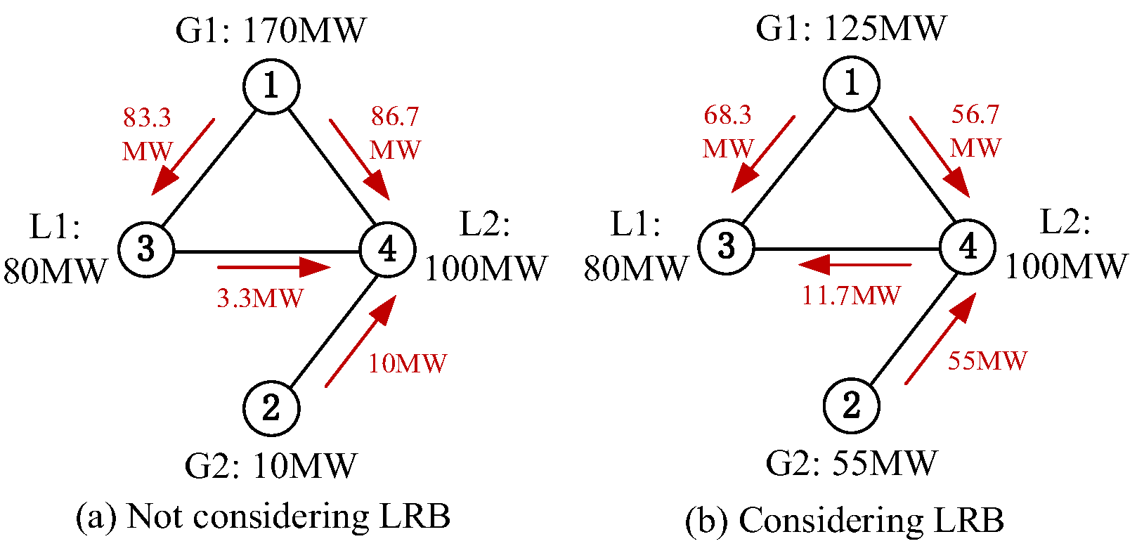
The LRB fundamentally reflects the risk of line overloads and the probability of cascading failures by quantifying the uniformity of power flow distribution in power systems. During normal operation, if the line loading rates are highly unbalanced (i.e., power flow entropy is high), some lines will operate close to their thermal stability limits over extended periods [30]. Once an N-1 contingency occurs, the redistributed power flow can easily cause these heavily loaded lines to become instantaneously overloaded, triggering protection misoperations and leading to cascading trips. In extreme weather or severe fault scenarios, high-risk areas often cover multiple system components. When N-k concurrent failures occur, the tripping of initially faulted components triggers large-scale power flow redistribution, subjecting the remaining lines to severe overloading stress [30,31]. Figure 1 illustrates the impact of the LRB indicator on the risk of line power flow limit violation under N-1 contingencies. Assume that all line reactance in Figure 1 is 0.1 p.u. and the line power flow limits are all 150 MW. The loads at Buses 3 and 4 are 80 MW and 100 MW, respectively. When the LRB indicator is not considered, the generator outputs at Buses 1 and 2 are 170 MW and 10 MW, respectively. When the LRB indicator is considered, the generator outputs are 125 MW and 55 MW, respectively. The pre-contingency power flows are shown in Figure 1, where a more balanced power flow distribution is observed in Figure 1b than in Figure 1a. In the case of a fault-induced trip of Line 1–4 or 1–3, the dispatch scheme corresponding to Figure 1a results in line power flow limit violations, whereas the scheme in Figure 1b remains secure under any single N-1 contingency.

3. Siting and Sizing Model of ESSs

In this section, an ESS planning model is constructed that considers both investment costs and operational simulation. The optimization objective of this model is to minimize the total system cost, which includes the average daily investment cost of ESSs and the operational and maintenance costs of typical days. The proposed model incorporates actual system operational characteristics at the ESS planning level, while considering uncertain wind and solar output scenarios at the operational level, thereby ensuring the flexible regulation and secure operation of renewable energy power systems.

3.1. Optimization Objective of ESS Planning

The optimization objective of ESS planning is to minimize the total cost over the power system planning horizon while simultaneously mitigating the risk of power flow violations, including the daily investment cost C_pur, typical daily maintenance cost C_m,s, and operation cost C_op,s, LRB, and LR, as shown in (5). Ω_S is the set of generation scenarios of wind farms (WFs) and photovoltaic power stations (PPSs). N_S is the number of typical days. α₁ and α₂ are weight coefficients. The investment cost of an ESS includes the procurement and installation costs of energy storage batteries and their auxiliary equipment, which is primarily determined by the energy capacity and power capacity of ESSs, as shown in (6) [19]. Parameters $p_e^{max}$ and $E_e^{max}$ represent the rated power and capacity of an ESS at bus e, respectively. Ω_E is the set of buses eligible for ESS configuration. c_p and c_e are the cost coefficients for power conversion and energy storage of ESSs, respectively. r is the investment discount rate. y is the service life of ESSs. The maintenance cost is primarily determined by the charging/discharging power of ESSs, as shown in (7). cₘ is the daily average maintenance cost. $p_{e,t,s}^{in}$ and $p_{e,t,s}^{out}$ represent the charging/discharging power of an ESS at bus e in scenario s, respectively. The operation cost for scenario s in (8) comprises the fuel cost C_fuel,s of generators and the penalty cost C_wp,s associated with wind and solar power curtailment.

$$Obj=\min C_{\mathrm{pur}}+{\displaystyle \frac{1}{N_{\mathrm{S}}}}\left({\displaystyle \sum _{s\in {\Omega }_{\mathrm{S}}}\left(C_{\mathrm{m},s}+C_{\mathrm{op},s}\right)}+{\displaystyle \sum _{s\in {\Omega }_{\mathrm{S}}}\left({\alpha }_{1}LR{B}_s+{\alpha }_{2}L{R}_s\right)}\right)$$

(5)

$$C_{\mathrm{pur}}={\displaystyle \frac{1}{365}}{\displaystyle \sum _{e\in {\Omega }_{\mathrm{E}}}\left(c_{\mathrm{p}}{p}_e^{\max }+c_{\mathrm{e}}{E}_e^{\max }\right)}{\displaystyle \frac{r{\left(1+r\right)}^y}{{(1+r)}^y-1}}$$

(6)

$$C_{\mathrm{m},s}={\displaystyle \sum _{e\in {\Omega }_{\mathrm{E}}}{c}_{\mathrm{m}}\left(p_{e,t,s}^{\mathrm{i}\mathrm{n}}+p_{e,t,s}^{\mathrm{out}}\right)}$$

(7)

$$C_{\mathrm{op},s}=C_{\mathrm{fuel},s}+C_{\mathrm{wp},s}$$

(8)

3.2. Constraints for ESS Planning

The decision variables in the ESS planning model include the station siting, power capacity, and energy capacity. Equations (9) and (10) represent the ESS planning budget, including limits on the number and capacity of ESSs. $u_i^{max}$ indicates whether ESS is installed at bus i, taking 1 if installed and 0 otherwise. $E_i^{max}$ represents the capacity of ESS installed at bus i. Ω_B is the bus set. $N_{ess}^{max}$ denotes the upper bound for the number of ESSs. E^max denotes the upper bound for the capacity of ESSs. M is a sufficiently large positive number. Equations (11) and (12) specify that the rated power and capacity of an ESS at bus e can be non-zero only if bus e is selected as a site for ESS deployment, respectively. Equation (13) limits the charging and discharging power of an ESS at time t in scenario s. Equation (14) expresses the relationship between $E_e^{max}$ and $p_e^{max}$. n_p is the power-to-capacity ratio.

$${\displaystyle \sum _{i\in {\Omega }_{\mathrm{B}}}{u}_i^{\mathrm{ESS}}}\le N_{\mathrm{ess}}^{\max }$$

(9)

$${\displaystyle \sum _{i\in {\Omega }_{\mathrm{B}}}{E}_i^{\max }}\le E^{\max }$$

(10)

$$0\le p_e^{\max }\le \mathrm{M}{u}_i^{\mathrm{ESS}}, \forall i\in {\Omega }_{\mathrm{B}},e\in {\Omega }_{\mathrm{E}}(i)$$

(11)

$$0\le E_e^{\max }\le \mathrm{M}{u}_i^{\mathrm{ESS}},\forall i\in {\Omega }_{\mathrm{B}},e\in {\Omega }_{\mathrm{E}}(i)$$

(12)

$$0\le p_{e,t,s}^{\mathrm{in}}\le p_e^{\max }, 0\le p_{e,t,s}^{\mathrm{out}}\le p_e^{\max },\forall t\in {\Omega }_{\mathrm{T}},e\in {\Omega }_{\mathrm{E}}$$

(13)

$$p_e^{\max }=n_p{E}_e^{\max },\forall t\in {\Omega }_{\mathrm{T}},e\in {\Omega }_{\mathrm{E}}$$

(14)

3.3. System Operational Constraint

First, the power supply and load need to be balanced during the scheduling period, as shown in (15). Ω_G, Ω_W, Ω_P, and Ω_B are the set of generators, WFs, PPSs, and buses, respectively. p_ij,t,s denotes the active power flow on line ij at time t in scenario s. p_g,t,s denotes the generation of generator g at time t in scenario s. p_w,t,s denotes the generation of WF w at time t in scenario s. p_p,t,s denotes the generation of PPS p at time t in scenario s. $p_{i,t,s}^{load}$ denotes the load amount connected on bus i at time t in scenario s. The reactive power at each bus should be balanced, as shown in (16). q_ij,t,s denotes the reactive power flow on line ij at time t in scenario s. q_g,t,s denotes the reactive output of generator g at time t in scenario s. $q_{i,t,s}^{load}$ denotes the reactive power load connected on bus i at time t in scenario s. $Q_{ij}^C$ and $Q_i^{sh}$ represent the line charging reactive power and the bus shunt reactive power, respectively. WFs, PPSs, and ESSs operate at unity power factor during each dispatch time step. Equation (17) adopts the linearized branch power flow [31]. Δθ_ij,t,s is the phase angle difference across line ij. $\Delta$V_ij,t,s is the voltage magnitude difference across line ij. B_ij and G_ij are the mutual susceptance and mutual conductance between buses i and j in the admittance matrix, respectively. Equations (18) and (19) represent the minimum up/down time constraints of generators, respectively. u_g,t,s denotes the operational state of generator g at time t. UT_g and DT_g are the minimum up/down time. Equations (20) and (21) represent the generator output limits and ramping constraints, respectively. $p_g^{min}$ and $p_g^{max}$ are the minimum and maximum active power output of generator g. $q_g^{min}$ and $q_g^{max}$ are the minimum and maximum reactive power output of generator g. RD_g and RU_g are the ramp-up and ramp-down rate limits. Equation (22) specifies that simultaneous charging and discharging of the selected ESS location are not permitted at time t. $u_{e,t,s}^{in}$ and $u_{e,t,s}^{out}$ denote the charging/discharging states of ESS e at time t. Equation (23) enforces that charging and discharging operations are permitted only if the corresponding charging or discharging state is active. Equation (24) denotes the dynamic balance of the state of charge (SoC). ηⁱⁿ and η^out are the charging and discharging efficiency. ΔT is the duration of a scheduling period. Equation (25) limits the value of SoC at time t in scenario s. ${SOC}_e^{min}$ and ${SOC}_e^{max}$ are the minimum and maximum SoC percentages. Equation (26) imposes a daily cycling condition, mandating that the SoC at the end of each scheduling period be equal to its initial value. To prevent lifespan degradation caused by frequent charging and discharging of ESSs, Equations (27) and (28) impose constraints on the minimum duration for maintaining a charging or discharging state. OT_e and IT_e are the minimum charging and discharging time limits. Equations (29) and (30) enforce that the generation from WFs and PPSs at time t in scenario s is bounded above by their maximum available dispatchable output.

$$\begin{array}{l}{\displaystyle \sum _{ij\in {\Omega }_{\mathrm{L}}}{p}_{ij,t,s}}+{\displaystyle \sum _{g\in {\Omega }_{\mathrm{G}}(i)}{p}_{g,t,s}}+{\displaystyle \sum _{w\in {\Omega }_{\mathrm{W}}(i)}{p}_{w,t,s}}+{\displaystyle \sum _{p\in {\Omega }_{\mathrm{P}}(i)}{p}_{p,t,s}}+{\displaystyle \sum _{e\in {\Omega }_{\mathrm{E}}(i)}\left(p_{e,t,s}^{\mathrm{out}}-p_{e,t,s}^{\mathrm{in}}\right)}\\ =p_{i,t,s}^{\mathrm{load}} ,\forall t\in {\Omega }_{\mathrm{T}},i\in {\Omega }_{\mathrm{B}}\end{array}$$

(15)

$${\displaystyle \sum _{ij\in {\Omega }_{\mathrm{L}}}\left(q_{ij,t,s}+Q_{ij}^{\mathrm{C}}\right)}+{\displaystyle \sum _{g\in {\Omega }_{\mathrm{G}}(i)}{q}_{g,t,s}}=q_{i,t,s}^{\mathrm{load}}+Q_i^{\mathrm{sh}},\forall t\in {\Omega }_{\mathrm{T}},i\in {\Omega }_{\mathrm{B}}$$

(16)

$$\left\{\begin{array}{l}{p}_{ij,t,s}=B_{ij}\Delta {\theta }_{ij,t,s}-G_{ij}\Delta V_{ij,t,s}\\ q_{ij,t,s}=G_{ij}\Delta {\theta }_{ij,t,s}+B_{ij}\Delta V_{ij,t,s}\end{array}\right., \forall t\in {\Omega }_{\mathrm{T}},ij\in {\Omega }_{\mathrm{L}}$$

(17)

$${\displaystyle \sum _{\tau =t}^{t+U{T}_g-1}{u}_{g,\tau ,s}}\ge U{T}_g(u_{g,t,s}-u_{g,t-1,s}),\forall t\in {\Omega }_T,g\in {\Omega }_G$$

(18)

$${\displaystyle \sum _{\tau =t}^{t+D{T}_g-1}\left(1-u_{g,\tau ,s}\right)}\ge D{T}_g(u_{g,t-1,s}-u_{g,t,s}),\forall t\in {\Omega }_T,g\in {\Omega }_G$$

(19)

$$\left\{\begin{array}{l}{p}_g^{\min }{u}_{g,t,s}\le p_{g,t,s}\le p_g^{\max }{u}_{g,t,s}\hfill \\ q_g^{\min }{u}_{g,t,s}\le q_{g,t,s}\le q_g^{\max }{u}_{g,t,s}\hfill \end{array}\right.,\forall t\in {\Omega }_T,g\in {\Omega }_G$$

(20)

$$-R{D}_g{u}_{g,t,s}\le p_{g,t,s}-p_{g,t-1,s}\le R{U}_g{u}_{g,t,s},\forall t\in {\Omega }_T,g\in {\Omega }_G$$

(21)

$$u_{e,t,s}^{\mathrm{in}}+u_{e,t,s}^{\mathrm{out}}\le u_i^{\mathrm{ESS}},\forall t\in {\Omega }_{\mathrm{T}},e\in {\Omega }_{\mathrm{E}}(i)$$

(22)

$$0\le p_{e,t,s}^{\mathrm{in}}\le \mathrm{M}{u}_{e,t,s}^{\mathrm{in}}, 0\le p_{e,t,s}^{\mathrm{out}}\le \mathrm{M}{u}_{e,t,s}^{\mathrm{out}},\forall t\in {\Omega }_{\mathrm{T}},e\in {\Omega }_{\mathrm{E}}$$

(23)

$$E_{e,t,s}=E_{e,t-1,s}+{\eta }^{\mathrm{in}}{p}_{e,t,s}^{\mathrm{in}}\Delta T-{\displaystyle \frac{p_{e,t,s}^{\mathrm{out}}}{{\eta }^{\mathrm{out}}}}\Delta T$$

(24)

$${\mathrm{SoC}}_e^{\min }{E}_e^{\max }\le E_{e,t,s}\le {\mathrm{SoC}}_e^{\max }{E}_e^{\max },\forall t\in {\Omega }_{\mathrm{T}},e\in {\Omega }_{\mathrm{E}}$$

(25)

$$E_{e,t=N_{\mathrm{T}},s}=E_{e,t=0,s}$$

(26)

$${\displaystyle \sum _{\tau =t}^{t+O{T}_e-1}{u}_{e,\tau ,s}^{\mathrm{out}}}\ge O{T}_e\cdot (u_{e,t,s}^{\mathrm{out}}-u_{e,t-1,s}^{\mathrm{out}}),\forall t\in {\Omega }_T,e\in {\Omega }_E$$

(27)

$${\displaystyle \sum _{\tau =t}^{t+I{T}_e-1}{u}_{e,\tau ,s}^{\mathrm{in}}}\ge I{T}_e\cdot (u_{e,t,s}^{\mathrm{in}}-u_{e,t-1,s}^{\mathrm{in}}),\forall t\in {\Omega }_T,e\in {\Omega }_E$$

(28)

$$0\le p_{w,t,s}\le {\tilde{p}}_{w,t,s},\forall t\in {\Omega }_{\mathrm{T}},w\in {\Omega }_{\mathrm{W}}$$

(29)

$$0\le p_{p,t,s}\le {\tilde{p}}_{p,t,s}, \forall t\in {\Omega }_{\mathrm{T}},p\in {\Omega }_{\mathrm{P}}$$

(30)

In the ESS planning model above, the objective function simultaneously pursues economic efficiency (minimizing investment and operation costs) and resilience (minimizing power flow entropy), which are inherently contradictory because improving resilience often requires more ESSs, increasing costs. To cap total investment, hard upper limits on ESS number and capacity are introduced as constraints. If these limits are inactive, the economy–resilience trade-off naturally balances within the budget. If active, the resilience enhancement is forcibly truncated by the budget, missing the optimal trade-off. The minimum charge/discharge time constraints introduced in (27) and (28) reduce frequent state switching and short-term shallow charge/discharge by enforcing a sustained duration for charging or discharging, thereby mitigating battery aging and extending the actual operational lifetime of ESSs. This lowers replacement and maintenance costs over the full lifecycle while also contributing to system operational stability, serving as an effective lifetime cost control measure. The selection of the minimum charge/discharge time should comprehensively consider the cycle life characteristics of batteries.

4. Model Transformation and Uncertainty Modeling

To enable a tractable solution, the absolute value terms in (1) and (3) are converted into mixed-integer linear constraints, as given by (31) and (32). The nonlinear absolute value terms in (1) are linearized by introducing auxiliary variable a_ij,t,s, resulting in (31).

$$\left\{\begin{array}{l}-\mathrm{M}(1-a_{ij,t})+R_{ij,t,s}\le {\displaystyle \frac{p_{ij,t,s}}{p_{ij}^{\max }}}\le R_{ij,t,s}+\mathrm{M}(1-a_{ij,t})\hfill \\ -\mathrm{M}{a}_{ij,t}+R_{ij,t,s}\le -{\displaystyle \frac{p_{ij,t,s}}{p_{ij}^{\max }}}\le R_{ij,t,s}+\mathrm{M}{a}_{ij,t}\hfill \\ 0\le R_{ij,t,s}\le 1\hfill \end{array}\right.$$

(31)

$$\left\{\begin{array}{l}{R}_{ij,t,s}-R_{t,s}^{\mathrm{av}}\le \Delta R_{ij,t,s}\hfill \\ -R_{ij,t,s}+R_{t,s}^{\mathrm{av}}\le \Delta R_{ij,t,s}\hfill \\ {\displaystyle \sum _{t\in {\Omega }_{\mathrm{T}}}{\displaystyle \sum _{ij\in {\Omega }_{\mathrm{L}}}\Delta R_{ij,t,s}}}\le LR{B}_s\hfill \end{array}\right.$$

(32)

For a minimization objective, if an absolute value term appears in a constraint that only requires a lower bound (and its coefficient is positive), a relaxed linearization method can be applied. In this case, the minimization objective will automatically force the variable to take the exact absolute value without introducing binary auxiliary variables, as shown in (3) and (32). However, if the absolute value term appears inside an absolute value constraint or requires exact equality, the relaxation method cannot satisfy the equality condition, and binary auxiliary variables must be introduced for exact piecewise linearization, as demonstrated in (1) and (31).

In this paper, the uncertainties of wind and solar power are characterized by chance constraints, as shown in (33). In this formulation, x represents the vector of decision variables, and ξ denotes the uncertain parameters. The function g(⋅) represents the constraints that are affected by uncertainties. The parameter ε defines the maximum allowable probability of constraint violation. To capture these uncertainties, wind and solar generation data under different typical days are sampled to form N sets of typical data. For each data set D_n, K-means clustering is applied to partition it into S cluster centers, yielding a total of N_S = N $\times$ S representative scenarios. Based on these N_S scenarios, the SAA method is employed to convert (33) into the deterministic mixed-integer linear form (34)–(38) [32]. The binary variables in the SAA chance constraint reformulation include z_n and z_n,s. Here, z_n indicates whether the nth typical scenario set is valid, and z_n,s indicates whether the cluster center s within the nth typical scenario set is valid. Therefore, there exists a logical relationship between z_n and z_n,s (1 for valid, 0 otherwise), as shown in (34), indicating that if the nth typical scenario set is invalid, then the cluster centers within it must also be invalid. When cluster center s is valid, both the set D_n to which cluster center s belongs and cluster center s itself must be valid simultaneously, and (35) and (36) hold accordingly. Equations (37) and (38) reflect the conservativeness of the chance-constrained programming. ε₁ and ε₂ respectively control the proportion of valid typical scenario sets and the proportion of valid cluster centers within a typical scenario set.

$$\mathbb{P}\{g(x,\xi )\le 0\}\ge 1-\epsilon$$

(33)

$$z_{n,s}\le z_n,\forall n=1,\dots ,N,s\in D_n$$

(34)

$$0\le p_{w,t,s}\le {\tilde{p}}_{w,t,s}+\mathrm{M}\left(1 -z_{n,s}\right),\forall t\in {\Omega }_{\mathrm{T}},w\in {\Omega }_{\mathrm{W}},n=1,\dots ,N,s\in D_n$$

(35)

$$0\le p_{p,t,s}\le {\tilde{p}}_{p,t,s}+\mathrm{M}\left(1-z_{n,s}\right),\forall t\in {\Omega }_{\mathrm{T}},p\in {\Omega }_{\mathrm{P}},n=1,\dots ,N,s\in D_n$$

(36)

$${\displaystyle \sum _{n=1}^N{z}_n}/N\ge 1-{\epsilon }_1,\forall n=1,\dots ,N$$

(37)

$${\displaystyle \sum _{s=1}^S{z}_{n,s}}/S\ge 1-{\epsilon }_2,\forall n=1,\dots ,N$$

(38)

In the above chance-constrained planning, a typical-day data sample set is first determined based on empirical experience to ensure that the typical-day data samples are not lost during the K-means clustering process, thereby allowing both the typical days and the key data cluster characteristics within the typical days to be reflected in the chance constraints.

5. Case Study

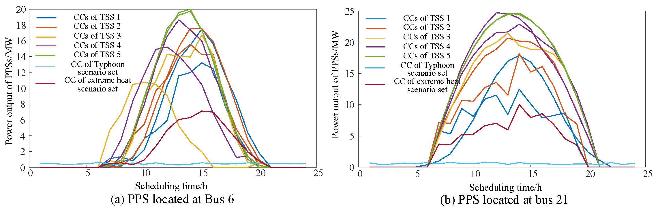
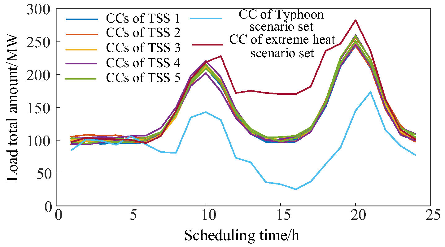
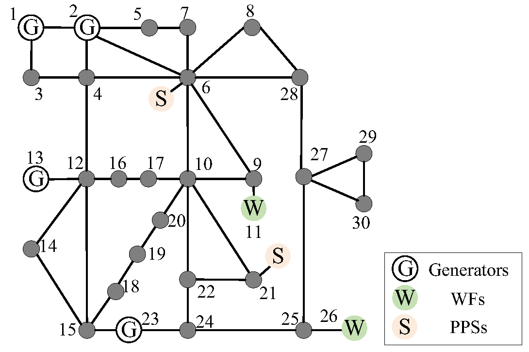
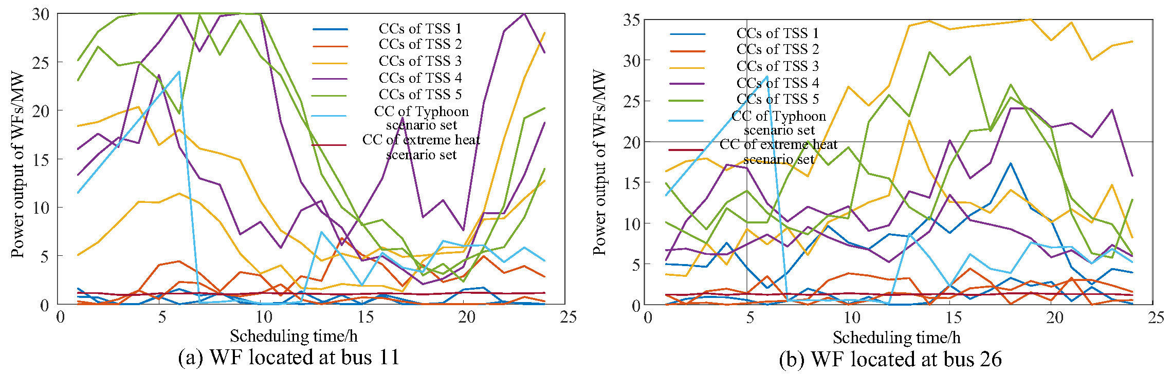
The effectiveness and practicality of the proposed ESS planning model are validated using the IEEE 30-bus standard test system, as shown in Figure 2. Two WFs are integrated at buses 11 and 26, respectively, while two PPS are connected at buses 6 and 21. The K-means clustering algorithm is applied to the typical and extreme scenario sets (TSSs and ESSs) of WFs, PPSs, and load total amount to generate representative cluster centers (CCs), which are illustrated in Figure 3, Figure 4 and Figure 5. The definition of scenarios and conditions is presented in

Table 2. Definition of scenarios and conditions.

Scenario Set Number	Conditions	Number of Cluster Centers
1	Typical	2
2	Typical	2
3	Typical	2
4	Typical	2
5	Typical	2
6	Typhoon	1
7	Extreme heat	1

. $N_{ess}^{max}$ and E^max are set to 3 and 120 MWh, respectively. The values of c_p, c_e, and c_m are taken as 50 $/kWh, 140 $/kWh, and 2 $/MWh, respectively. The values of r and y are taken as 6% and 15. ${SOC}_e^{min}$ and ${SOC}_e^{max}$ are set to 0.1 and 0.9, respectively. ηⁱⁿ and η^out are set to 0.95.

5.1. Siting and Sizing Results and Scheduling Schemes of ESSs

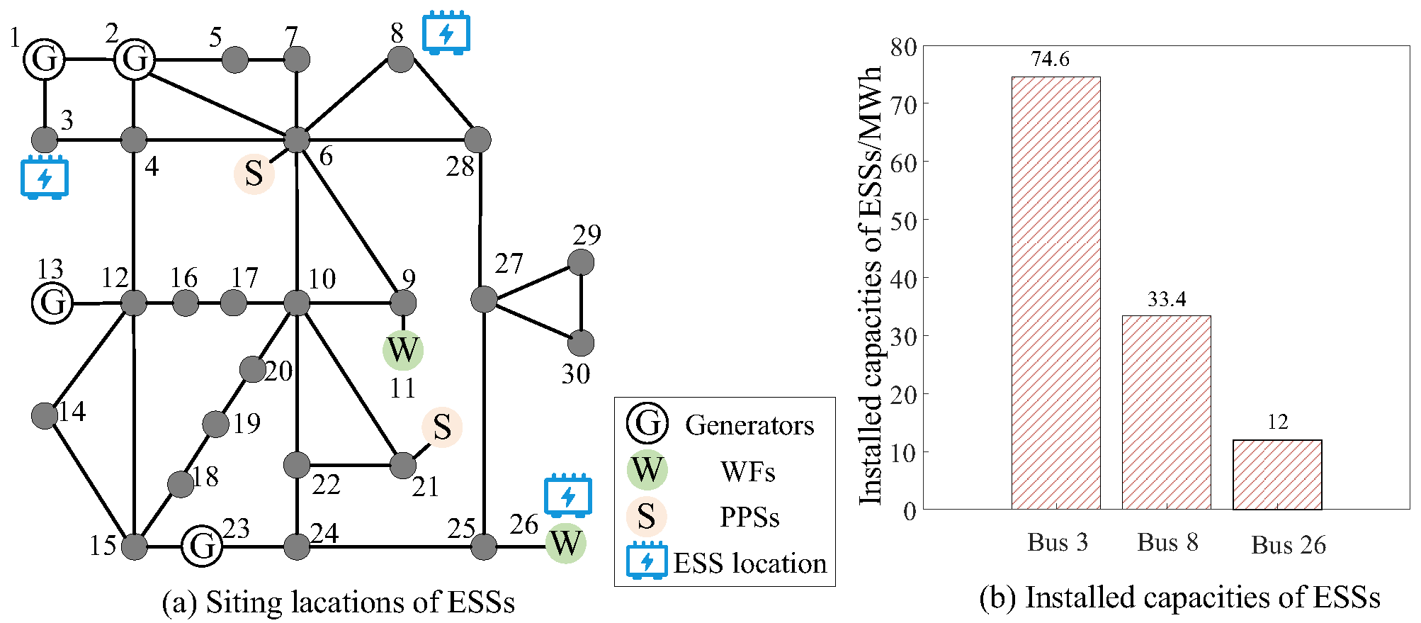
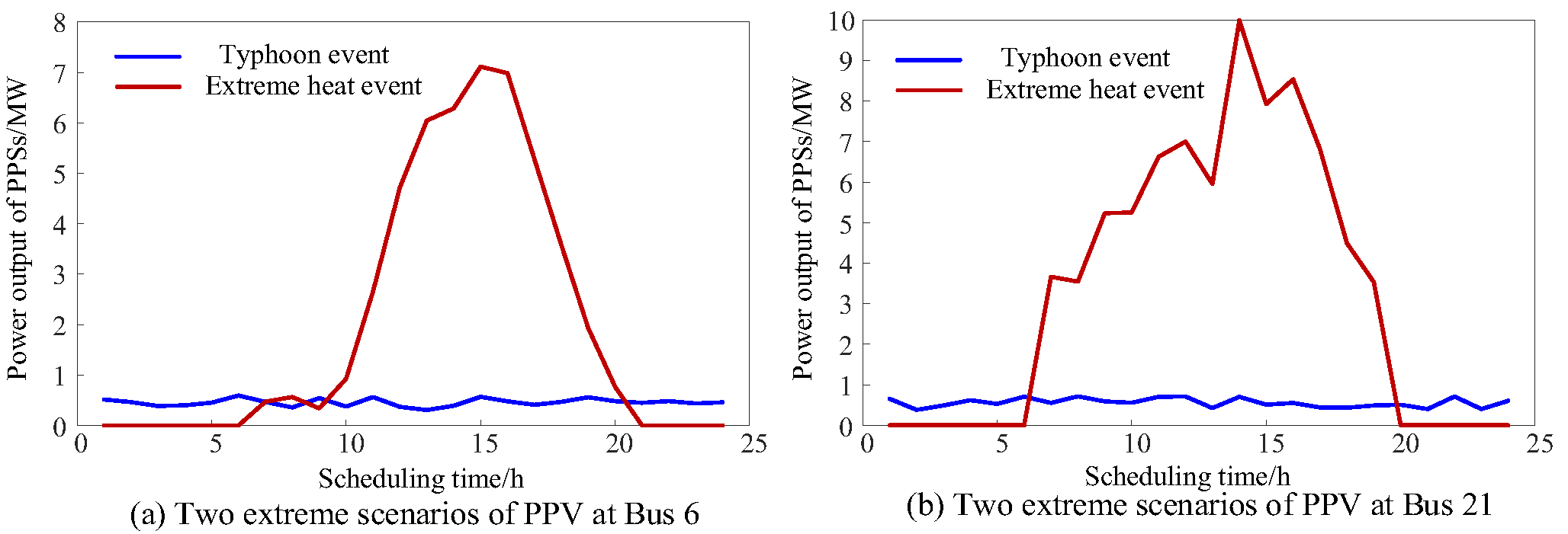
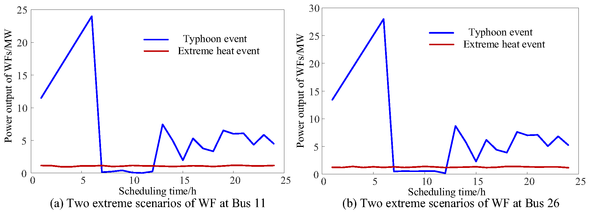
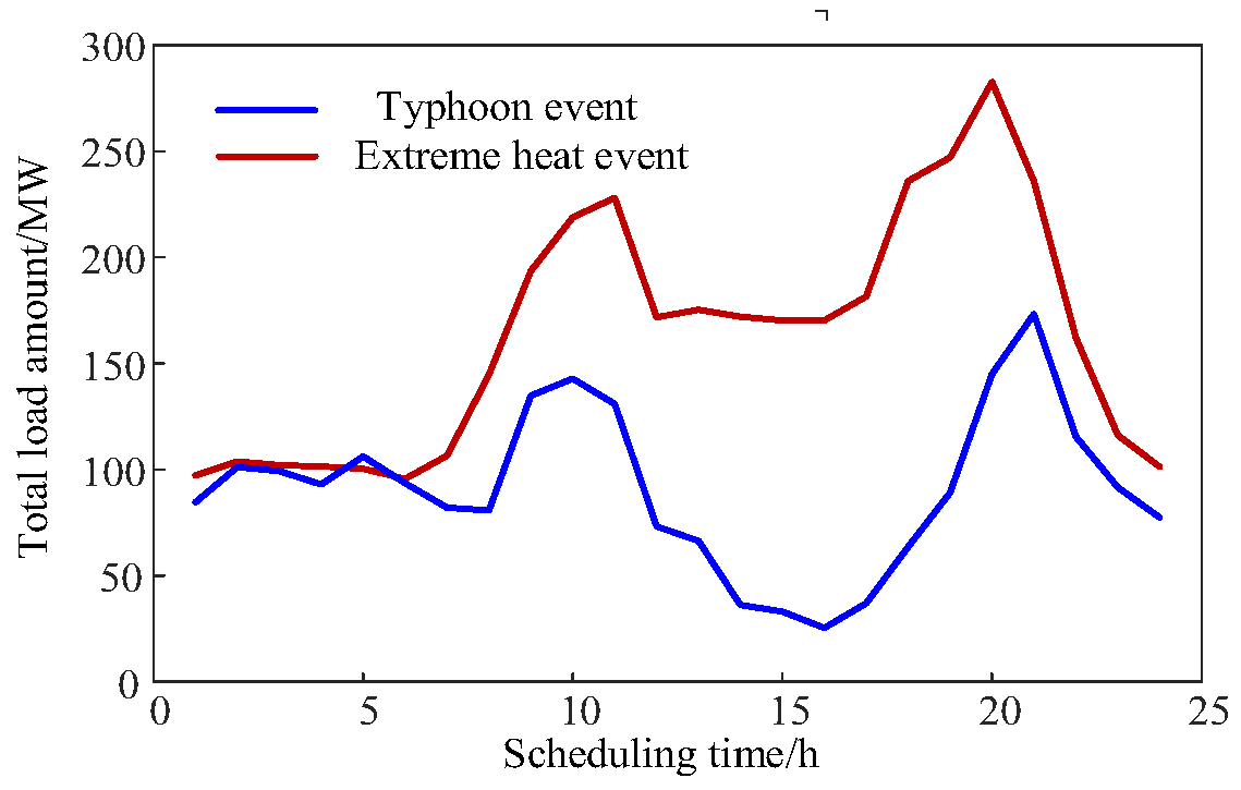
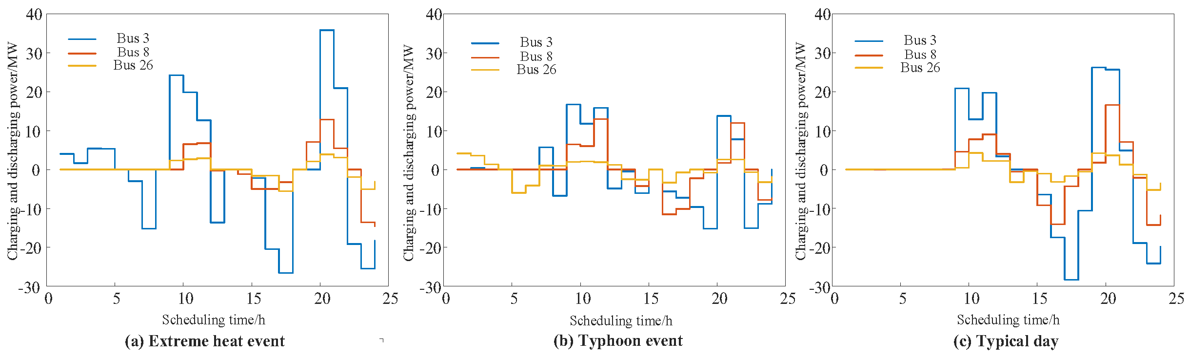
Chance-constrained planning parameter ε is set to 0.1, n_p is set to 0.5. Based on the above parameter configuration, the siting locations and installed capacities of ESSs are obtained, as shown in Figure 6. From Figure 6a, it can be seen that when the siting locations of ESSs are not restricted, ESSs can be sited at transmission buses, load buses, WFs, or even power plants, in order to balance the power flow and smooth the fluctuations of REGs. In Figure 6b, the total capacity of ESSs is 120 MW, reaching the upper limit of capacity planning. According to the ESS planning results, the rated power is limited to 37.31 MW, 16.71 MW, and 6 MW, respectively. The ESS scheduling schemes under different scenarios, derived from the ESS planning method proposed in this paper, are demonstrated by selecting an extreme heat scenario, a typhoon scenario, and a typical scenario. The typical scenario is selected according to the severity of fluctuations in renewable energy output. Figure 7, Figure 8 and Figure 9 present the outputs of PPSs and WFs, as well as the total load, under typhoon and extreme heat scenarios. In typhoon scenarios, dense clouds and heavy rain drastically reduce solar irradiance, making PV output nearly zero, while wind speed fluctuates dramatically, and the total load decreases due to facility shutdowns and reduced human activity. In extreme heat scenarios, PV output declines primarily because of the negative temperature coefficient of photovoltaic cells, whereas the total load increases sharply driven by higher electricity demand for cooling, and there is little to no wind. Figure 10 shows the charging/discharging schemes of ESSs. It can be seen that under extreme heat scenarios, although the fluctuations of WFs and PPSs are relatively small, the total load fluctuates significantly, and the charging and discharging power of ESSs reach their rated values. Under typhoon scenarios, the total load fluctuates relatively little, so the charging and discharging power of ESSs is also small. As can be seen from

Table 3. Daily dispatch costs for three selected extreme scenarios.

Scenario Number	Cpur/$	Cm,s/$	Cfuel,s/$	Cwp,s/$	Total Costs/$
Extreme heat event	5585.4	782	8175.8	516	15,059.2
Typhoon event		566.3	3694.8	1907.5	11,753.7
Typical day		769.2	5426.3	7472	19,252.9

, under the extreme heat scenario, the operating costs of ESSs and conventional generators are the highest, while under the typical scenario, the costs of wind and solar curtailment and the total cost are the highest.

5.2. Sensitivity Analysis of Model Parameters

The power-to-capacity ratio n_p dictates the relationship between power and energy capacity of ESSs. A larger n_p prioritizes power-oriented uses with rapid response, and a smaller n_p lends itself to energy-oriented uses for prolonged support.

Table 4. Resulting planning schemes for typical n_p values.

Type	Values of np	Siting Locations	Installed Capacities/MWh	Cpur/$
Capacity-oriented	0.5	Buses 3, 8, 26	74.6, 33.4, 12	5585
Hybrid	1	Buses 1, 8, 26	76.4, 29.6, 14	6432
Power-oriented	2	Buses 1, 8, 26	71.3, 36.6, 12.1	8124

compares the resulting planning schemes for typical n_p values. It can be seen that the choice of n_p significantly affects the optimal siting and sizing of ESSs. The rated power of ESSs limits their short-term regulation capability, while the rated capacity limits their long-term regulation capability. From the increasing trend of ESS investment costs in Table 4, it can be seen that the capacity budget constraint remains active for all different values of n_p, indicating that the regulation capability of ESSs during typical daily operation may be constrained by both their rated power and rated capacity.

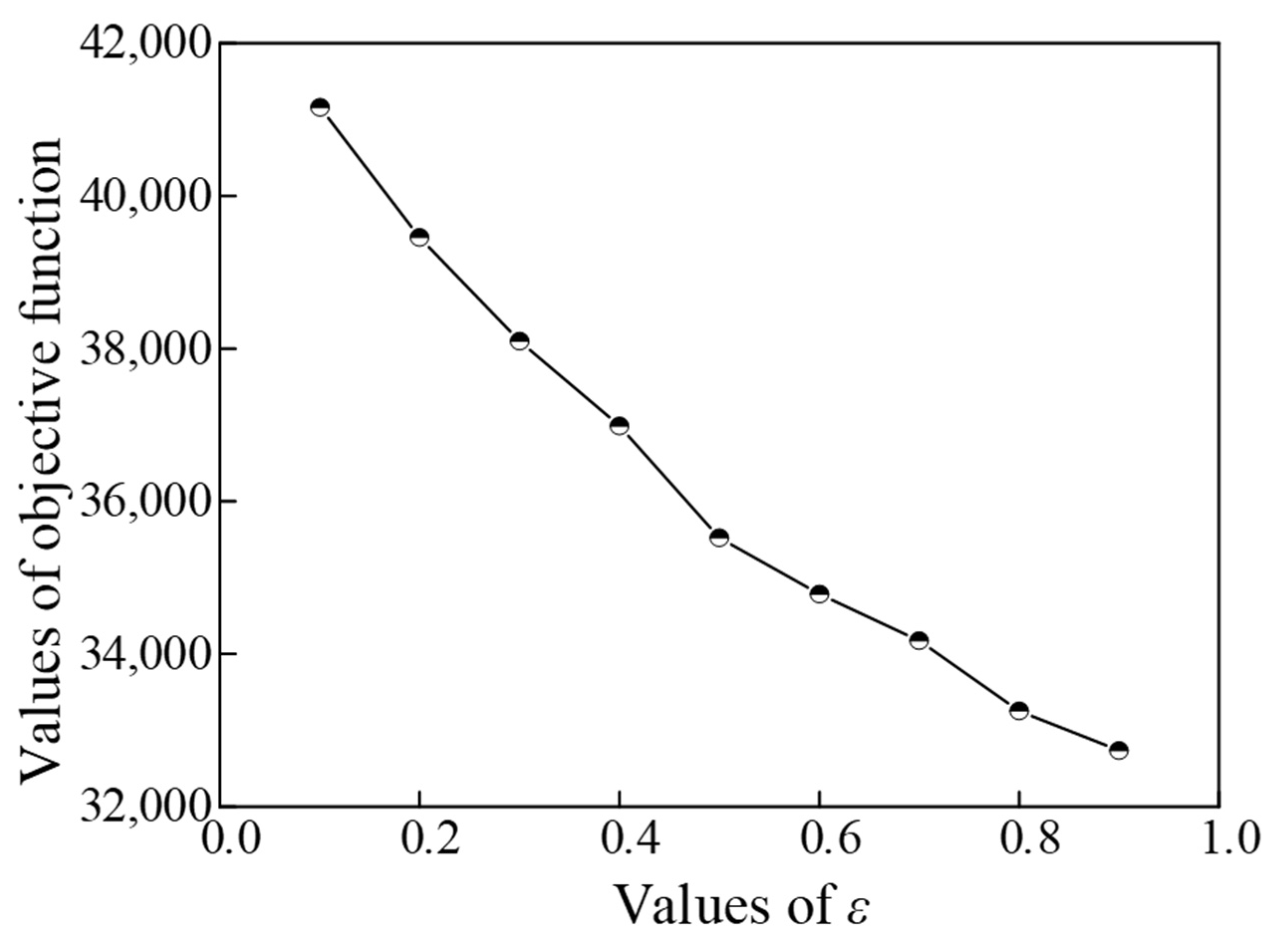
Parameter ε determines the conservativeness of the chance-constrained planning model. A larger value of ε lowers the probability that the solution can adequately cope with the uncertainties of wind and solar power, whereas a smaller ε deteriorates both the expected economic performance and the resilience indicator of the solution. Figure 11 depicts the variation in the objective function value with respect to the parameter ε. In this paper, a smaller objective function value indicates better economic performance and resilience indicator. It can be observed that as the value of ε increases, the objective function value gradually decreases, demonstrating the impact of the uncertainty budget parameter on the conservativeness of the solution.

Furthermore, the selection of the weight coefficient of resilience indicators may affect the ESS planning and system dispatch operation costs. Therefore, it is necessary to analyze the impact of the weight coefficient α on the economic performance of planning and dispatch.

Table 5. ESS planning and operation costs under different weight coefficient α.

α	Planning Cost/$	Expected Operation Cost/$
0	5585	11,094
0.5	5585	11,104
5	5585	11,428
10	5585	11,479
50	5585	16,564

shows the ESS planning cost and the expected system operation cost under different weight coefficients. It can be observed that different coefficients have negligible effects on the planning costs, because the selected number and capacity limits of ESSs are both hard constraints in the optimization. Therefore, the planned number and capacity remain the same under different coefficients. In addition, the operation cost gradually increases as the coefficient of resilience indicators increases. However, this increase becomes significant only when the value of α reaches a certain threshold. By selecting appropriate weight coefficients, the resilience indicators can be improved without significantly compromising economic performance.

5.3. Scheme Comparison to Validate the Effectiveness of Considering LRB

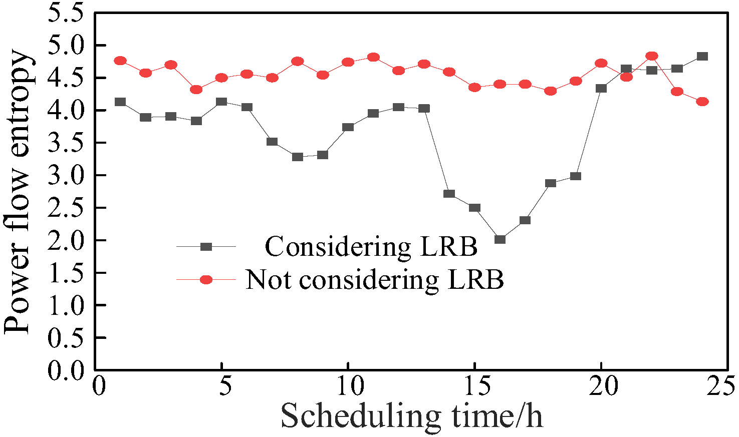
To illustrate the impact of incorporating LRB on ESS planning schemes and subsequent dispatch schemes, α₁ and α₂ are both set to zero to generate the LRB-excluded schemes, which are then compared with those including the LRB.

Table 6. ESS planning schemes with and without considering LRB.

LRB	Siting Locations	Installed Capacities/MWh	Daily Investment Cost/$
Considering	Buses 3, 8, 26	74.6, 33.4, 12	5585
Not considering	Buses 3, 8, 26	55.6, 48, 16.4	5585

presents the differences between ESS planning schemes with and without considering LRB. Figure 9 compares the power flow entropy of the dispatch schemes with and without considering LRB. It can be seen from Table 6 that the ESS location does not change while the planned ESS capacity changes significantly after considering LRB, under the premise that the daily investment cost remains unchanged. As shown in Figure 12, under the selected typical scenario, the daily dispatch costs with and without considering LRB are $11,104 and $11,094, respectively. It can be observed that, with almost no impact on economic efficiency, the proposed model can significantly improve LRB, thereby enhancing the safety and resilience of the dispatch schemes.

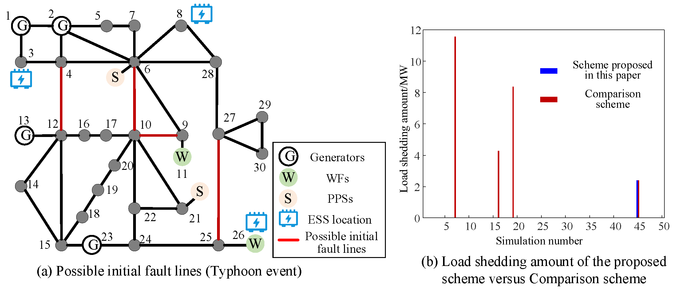
The possible initial fault lines are selected as Line 4–12, Line 6–10, Line 9–10 and Line 25–27, which can be found in Figure 13a. Monte Carlo simulation is used to simulate initial line outages. In this paper, the initial line outage is set as N-2, and the number of simulations is set to 50. The impact of line outages on fault propagation is reflected by the load shedding amount. The load shedding amounts of the proposed scheme and the comparison scheme are shown in Figure 13b. It can be observed that after incorporating the proposed resilience indicator, the load shedding amounts is significantly reduced under most simulations of random N-2 faults.

6. Conclusions

Aiming to enhance the dispatch revenue of ESSs in complex environments and their support capability for the safety and resilience requirements of power systems, this paper proposes an ESS planning model that considers the uncertainties of REGs and resilience requirements for extreme events. A coordinated ESS planning and dispatch optimization model is formulated to minimize the equivalent daily planning cost, daily dispatch cost, and LRB, subject to secure operation constraints of the power system under renewable generation uncertainties. The uncertainty risks of REGs are mitigated via SAA-based chance-constrained planning within the daily dispatch cycle, LRB is characterized by the sum of absolute deviations of loading rates, and this indicator is linearized to facilitate solution. The simulation results demonstrate that:

(1) The proposed ESS planning method can significantly improve the LRB resilience indicator of the system under extreme scenarios without increasing the planning cost and with almost no increase in operational cost.

(2) By comparing the ESS planning schemes obtained with and without considering the LRB indicator, together with the corresponding dispatch schemes under N-k extreme scenario simulations, it is shown that an enhanced LRB indicator can significantly reduce load shedding under extreme scenarios.

(3) In the SAA-based chance-constrained programming, a trade-off between the ESS planning cost and system resilience under the combined influence of typical and extreme source-load uncertainty scenarios can be achieved by adjusting conservative threshold parameter.

References

1. Global Energy in 2026: Growth, Resilience and Competition. Available online: https://www.weforum.org/stories/2025/12/global-energy-2026-growth-resilience-and-competition/ (accessed on 18 March 2026).
2. Electricity 2026. Available online: https://www.iea.org/reports/electricity-2026 (accessed on 18 March 2026).
3. Dong, W.; Chen, X.; Yang, Q. Data-driven scenario generation of renewable energy production based on controllable generative adversarial networks with interpretability. Appl. Energy 2022, 308, 118387. [Google Scholar] [CrossRef]
4. Wang, Z.; Niu, T.; Fang, S.; Chen, G.; Feng, N.; Feng, Y.; Xue, L. Convex hull approximation of probabilistic security region of bulk power system with high renewable energy penetration considering N–k contingencies. IEEE Trans. Power Syst. 2025, 40, 4882–4900. [Google Scholar] [CrossRef]
5. Dobson, I. Models, metrics, and their formulas for typical electric power system resilience events. IEEE Trans. Power Syst. 2023, 38, 5949–5952. [Google Scholar] [CrossRef]
6. Stanković, A.M.; Tomsovic, K.L.; De Caro, F.; Braun, M.; Chow, J.H.; Čukalevski, N.; Dobson, I.; Eto, J.; Fink, B.; Hachmann, C.; et al. Methods for analysis and quantification of power system resilience. IEEE Trans. Power Syst. 2023, 38, 4774–4787. [Google Scholar] [CrossRef]
7. Yan, S.; Shen, Q.; Li, X.; Li, S.; Chu, E. SOC balancing control based on multi-agent for multiple energy storage units in MMC high power energy storage system. CSEE J. Power Energy Syst. 2025, 11, 1253–1261. [Google Scholar]
8. Tao, S.; Tan, Z.; Yang, C.; Yan, Z.; Cheng, H. Path-aware market clearing model for inter-regional electricity market via redundancy elimination. J. Mod. Power Syst. Clean. Energy 2024, 12, 1980–1992. [Google Scholar] [CrossRef]
9. Yan, C.; Geng, X.; Bie, Z.; Xie, L. Two-stage robust energy storage planning with probabilistic guarantees: A data-driven approach. Appl. Energy 2022, 313, 118623. [Google Scholar] [CrossRef]
10. Xiong, P.; Singh, C. Optimal planning of storage in power systems integrated with wind power generation. IEEE Trans. Sustain. Energy 2016, 7, 232–240. [Google Scholar] [CrossRef]
11. Wang, S.; Geng, G.; Jiang, Q. Robust co-planning of energy storage and transmission line with mixed integer recourse. IEEE Trans. Power Syst. 2019, 34, 4728–4738. [Google Scholar] [CrossRef]
12. Guo, Z.; Wei, W.; Chen, L.; Shahidehpour, M.; Mei, S. Economic value of energy storages in unit commitment with renewables and its implication on storage sizing. IEEE Trans. Sustain. Energy 2021, 12, 2219–2229. [Google Scholar] [CrossRef]
13. Wang, Q.; Zhang, X.; Yi, C.; Li, Z.; Xu, D. A novel shared energy storage planning method considering the correlation of renewable uncertainties on the supply side. IEEE Trans. Sustain. Energy 2022, 13, 2051–2063. [Google Scholar] [CrossRef]
14. Cao, X.; Cao, T.; Gao, F.; Guan, X. Risk-averse storage planning for improving RES hosting capacity under uncertain siting choices. IEEE Trans. Sustain. Energy 2021, 12, 1984–1995. [Google Scholar] [CrossRef]
15. Wang, X.; Li, F.; Zhang, Q.; Shi, Q.; Wang, J. Profit-oriented BESS siting and sizing in deregulated distribution systems. IEEE Trans. Smart Grid 2023, 14, 1528–1540. [Google Scholar] [CrossRef]
16. Abdeltawab, H.; Mohamed, Y.A.-R.I. Mobile energy storage sizing and allocation for multi-services in power distribution systems. IEEE Access 2019, 7, 176613–176623. [Google Scholar] [CrossRef]
17. Li, J.; Xu, Z.; Liu, H.; Wang, C.; Wang, L.; Gu, C. A Wasserstein distributionally robust planning model for renewable sources and energy storage systems under multiple uncertainties. IEEE Trans. Sustain. Energy 2023, 14, 1346–1356. [Google Scholar] [CrossRef]
18. Ghatak, S.; Sannigrahi, S.; Parimal, A. Optimized planning of distribution network with photovoltaic system, battery storage, and DSTATCOM. IET Renew. Power Gener. 2018, 12, 1823–1832. [Google Scholar] [CrossRef]
19. Abdeltawab, H.; Mohamed, Y.A.-R.I. Energy storage planning for profitability maximization by power trading and ancillary services participation. IEEE Syst. J. 2022, 16, 1909–1920. [Google Scholar] [CrossRef]
20. Yao, M.; Cai, X.; Vicino, A. Energy storage sizing optimization for large-scale PV power plant. IEEE Access 2021, 9, 75599–75607. [Google Scholar] [CrossRef]
21. Ma, G.; Li, J.; Zhang, X.-P. Energy storage capacity optimization for improving the autonomy of grid-connected microgrid. IEEE Trans. Smart Grid 2023, 14, 2921–2933. [Google Scholar] [CrossRef]
22. Wu, L.; Geng, Y.; Xue, X.; Xu, J.; Chen, X. Grid-forming energy storage capacity allocation considering transient power support. In Proceedings of the 2025 5th International Conference on Mechanical, Electronics and Electrical and Automation Control, Chongqing, China, 9–11 May 2025. [Google Scholar]
23. She, B.; Wu, D.; Kwon, K. A review of energy storage for power system resilience: Functions, metrics, and applications. Appl. Energy 2026, 420, 128056. [Google Scholar] [CrossRef]
24. Nazemi, M.; Moeini-Aghtaie, M.; Fotuhi-Firuzabad, M.; Dehghanian, P. Energy storage planning for enhanced resilience of power distribution networks against earthquakes. IEEE Trans. Sustain. Energy 2020, 11, 795–806. [Google Scholar] [CrossRef]
25. Huang, W.; Zhang, X.; Li, K.; Zhang, N.; Strbac, G.; Kang, C. Resilience oriented planning of urban multi-energy systems with generalized energy storage sources. IEEE Trans. Power Syst. 2022, 37, 2906–2918. [Google Scholar] [CrossRef]
26. Zhang, B.; Gong, C.; Fan, S.; Wang, J.; Yu, T.; Wang, Z. Research on mobile energy storage configuration and path planning strategy under dual source-load uncertainty in typhoon disasters. Energies 2025, 18, 5169. [Google Scholar] [CrossRef]
27. Bingkai, H.; Yuxiong, H.; Qianwen, H.; Gengfeng, L.; Zhaohong, B. Distributionally robust allocation of energy storage integrated with soft open points coordinating flexibility and resilience. IET Gener. Transm. Distrib. 2025, 19. [Google Scholar] [CrossRef]
28. Yang, H.; Zhang, C.; Li, J.; Zhu, L.; Zhou, K. A novel robust energy storage planning method for grids with wind power integration considering the impact of hurricanes. IEEE Trans. Sustain. Energy 2025, 16, 1388–1400. [Google Scholar] [CrossRef]
29. Cao, S.; Zhang, X.; Xiang, W.; Wen, J. A power flow transfer entropy based AC fault detection method for the MTDC wind power integration system. IEEE Trans. Ind. Electron. 2021, 68, 11614–11620. [Google Scholar] [CrossRef]
30. Wang, Y.; Huang, L.; Shahidehpour, M.; Lai, L.L.; Yuan, H.; Xu, F.Y. Resilience-constrained hourly unit commitment in electricity grids. IEEE Trans. Power Syst. 2018, 33, 5604–5614. [Google Scholar] [CrossRef]
31. Gu, X.; Bai, Y.; Li, S.; Liu, K.; Liu, Y.; Wang, H. An optimisation method of whole-process restoration decision-making of power systems considering disturbance-resisting ability of the restored network. IET Gener. Transm. Distrib. 2023, 17, 1638–1651. [Google Scholar] [CrossRef]
32. Kleywegt, J.; Shapiro, A.; Homem-de-Mello, T. The sample average approximation method for stochastic discrete optimization. SIAM J. Optim. 2002, 12, 479–502. [Google Scholar] [CrossRef]
Figure 1. Influence of LRB indicator on the risk of line power flow limit violation.
Processes 14 02067 g001
Figure 2. IEEE 30-bus system topology.
Processes 14 02067 g002
Figure 3. Representative cluster centers obtained by K-means method of WFs.
Processes 14 02067 g003
Figure 4. Representative cluster centers obtained by K-means method of PPSs.
Processes 14 02067 g004
Figure 5. Representative cluster centers obtained by K-means method of total load amount.
Processes 14 02067 g005
Figure 6. Planning results of ESSs.
Processes 14 02067 g006
Figure 7. Two extreme scenarios of PPSs.
Processes 14 02067 g007
Figure 8. Two extreme scenarios of WFs.
Processes 14 02067 g008
Figure 9. Two extreme scenarios of loads.
Processes 14 02067 g009
Figure 10. Scheduling schemes of ESSs.
Processes 14 02067 g010
Figure 11. Objective function values for different ε.
Processes 14 02067 g011
Figure 12. Power flow entropy of dispatch schemes under typical scenarios with and without considering LRB.
Processes 14 02067 g012
Figure 13. The proposed scheme versus Comparison scheme under N-2 initial fault simulation.
Processes 14 02067 g013