A New Decomposition Method for Split-Film Thermoanemometry Probes

Abstract

This paper presents a novel decomposition method for split-film probes to improve pitch angle determination over a wide range of flow velocities. Conventional approaches often suffer from the velocity dependence of the directional response function, resulting in large angular errors. The proposed method introduces a new functional formulation based on effective cooling velocities and velocity-dependent reference parameters. These parameters are explicitly derived from calibration data and modeled using fourth-order polynomial regressions to suppress velocity-induced variance. Experimental verification conducted for velocities between 2.2 and 14.6 m/s demonstrates that the proposed method collapses the calibration data more effectively than previous models. The total angular estimation error does not exceed ±2° within the pitch angle range from −60° to 60°. The proposed approach is therefore suitable for reliable measurements in low-velocity regions of complex flows, such as wakes and recirculation zones.

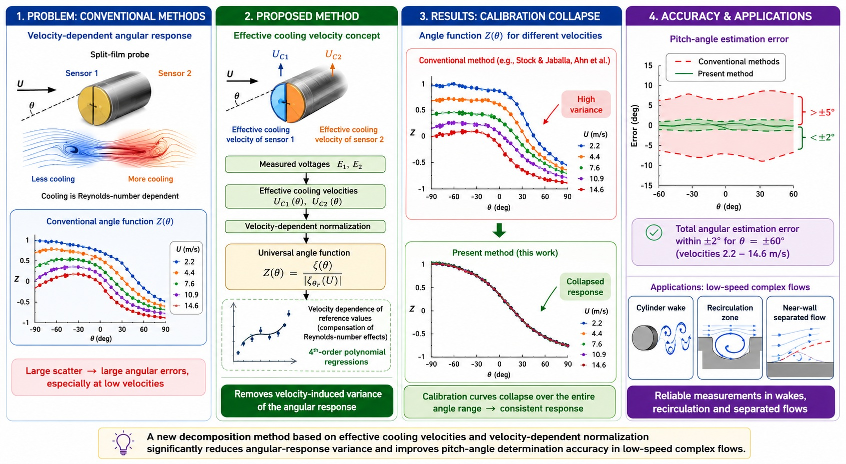
1. Introduction

A split-film probe is used for two-dimensional flow measurement by means of thermal anemometry. The operating principle is based on convective heat transfer. The probe consists of a thermally sensitive film divided into two electrically independent segments. When the sensors are electrically heated by a two-channel thermal anemometer, the surrounding fluid removes heat at a rate dependent on the local flow conditions. The resulting electrical signals from the two film segments are therefore functions of both the velocity magnitude (U) and the pitch angle ($\theta$).

Measurements of complex flow characteristics, commonly performed by traditional X-wire probes, can also be performed by a split-film probe [1]. The split-film sensor offers several distinct advantages over conventional hot-wire probes. Its significantly smaller physical size leads to improved spatial resolution, particularly in regions characterized by strong velocity gradients. This compact design also allows for measurements much closer to the surfaces than is possible with standard hot-wire anemometry. It is able to detect forward/reverse flow in separated regions [2]. An important advantage of the film sensor is its robustness. The split-film probe has been successfully used in demanding environments, where classical hot-wire probes are highly vulnerable to dust particle impact (e.g., for measuring unsteady flow characteristics in a compressor [3]). The split-film probe can be used not only in gaseous flows but also in liquid environments [4]. This is enabled by a protective quartz coating applied to the sensing elements, which provides electrical insulation while preserving the thermal sensitivity of the sensor. As a result, the split-film probe can operate in conductive fluids, including environments that are not chemically inert. This extended applicability significantly broadens the range of potential uses of split-film anemometry beyond air flows. These include liquid-phase transport processes, mixing studies, and measurements in industrial process equipment.

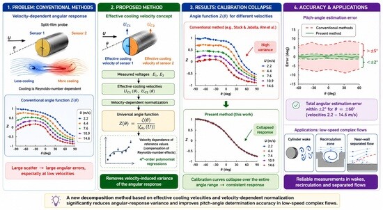
Despite these advantages, split-film anemometry requires more complex calibration procedures. Its directional response generally depends on the flow velocity. Decomposition methods employ an angle function to extract the flow angle from the sensor outputs. However, conventionally used angle functions tend to lose accuracy at low flow velocities. To address this limitation, a new form of angle function has been proposed that remains applicable over a substantially wider velocity range.

2. Theoretical Background

In many practical applications, such as wakes behind bluff bodies, recirculation regions, or near-wall separated flows, the local velocity can be significantly lower than the free-stream value. In these regions, the probe operates at Reynolds numbers well below the range where existing methods perform reliably, as will be discussed in Section 2.4. Developing a calibration and evaluation methodology that remains accurate in the velocity range covering both subcritical and supercritical regimes is essential for reliable measurements in low-velocity and highly unsteady flows.

2.1. Thermal Anemometer

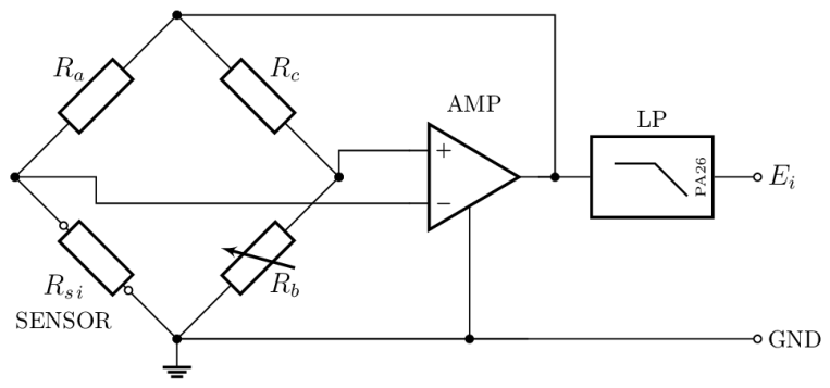
A thermal anemometer is a measuring instrument that supplies electrical power to a heated sensor and generates an output voltage signal proportional to its convective cooling. The anemometer operates in constant-temperature mode (CTA) by maintaining the sensor at a constant temperature higher than that of the surrounding fluid. The sensor of a probe is connected as one arm of a Wheatstone bridge circuit, as illustrated in Figure 1. To set the sensor’s operating temperature, the system maintains its corresponding electrical resistance $R_s$. Under balanced bridge conditions, this sensor resistance is determined by and proportional to the reference resistance $R_b$ adjusted on the bridge.

When fluid flows over the heated sensor, convective heat transfer increases, which would otherwise cool the sensor. To prevent any actual drop in temperature, the feedback loop immediately detects the transient change in electrical resistance as a bridge imbalance, and the feedback amplifier (AMP) adjusts the heating current to maintain equilibrium. By continuously regulating this current, the system keeps the sensor’s temperature and resistance constant. The bridge voltage required to maintain this thermal state is directly related to the velocity of the fluid flow. Finally, the anemometer’s signal conditioner provides low-pass (LP) filtering to serve as an anti-aliasing filter prior to digital data acquisition. The anemometer output voltage corresponding to the sensor $E_i$—simply referred to as the “sensor voltage”—serves as the primary measured variable in thermal anemometry.

2.2. Convective Heat Transfer Around the Split-Film Sensor

The heat transfer between the heated sensor and the surrounding fluid is described by Newton’s cooling law:

$$Q=hA(T_s-T_a),$$

(1)

where Q is the convective heat flux, h is the convective heat-transfer coefficient, A is the heat-transfer area, $T_s$ is the sensor temperature, and $T_a$ is the fluid temperature. The magnitude and spatial distribution of the heat-transfer coefficient around a cylindrical sensor depend [5] on the Reynolds number:

$$Re={\displaystyle \frac{UD}{\nu }},$$

(2)

where U is the flow velocity, D is the sensor diameter, and $\nu$ is the kinematic viscosity taken at the temperature corresponding to the arithmetic mean of the sensor and flow temperatures.

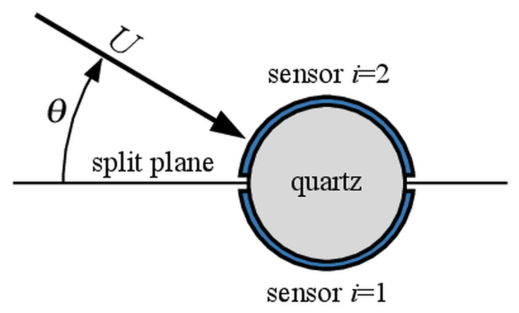
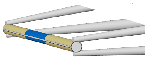
Each segment of split-film sensor (see Figure 2 and Figure 3) is exposed to a different integrated cooling intensity depending on the local heat-transfer distribution. The output voltage of each segment can consequently be interpreted as a measure of the integrated convective cooling over the corresponding sensor surface region:

$$E_i^2\sim {\int }_{{\Gamma }_i}h(\varphi ,Re)d\varphi ,$$

(3)

where ${\Gamma }_i$ denotes the surface region occupied by the individual split-film segment, and $\varphi$ is the circumferential coordinate around the cylinder.

2.3. Velocity Dependence of the Angle Function

The reasons for the velocity dependence of the angle function, derived from sensor voltages, arise from the physical phenomena that occur on a cylindrical sensor in cross-flow. The signals of a split-film probe are proportional to the convective heat transfer from each of the two sensing elements located on opposite sides of the cylinder. However, the distribution of time-averaged local heat transfer around a heated cylinder depends on the Reynolds number. The flow remains steady up to $R{e}_c\approx 40$, which corresponds to the critical Reynolds number for the onset of vortex shedding. As the Reynolds number increases, periodic vortex structures enhance mixing and significantly increase heat transfer on the rear side of the cylinder. For a given flow angle, the ratio of the signals measured by the two sensors varies with Reynolds number, reflecting the increasing influence of unsteady wake dynamics.

2.4. Overview of Existing Split-Film Methods

Determining the flow direction from a split film probe has historically evolved into several methodologies. The method presented by Stock and Jaballa (1985) [6] utilizes an angle function $Z_A$, normalized by reference sensor calibration, to determine the pitch angle. This approach is simple and performs well at small pitch angles. However, later analysis of the method [7] concludes that changes in the velocity magnitude produce a scatter of data, which means the angle function used is actually also dependent on the flow velocity $Z_A(\theta ,U)$.

To suppress the velocity dependence of directional response, Ra et al. [7] modified the method by expressing the angle function as the product of an angle-specific and the velocity magnitude function $Z_A(\theta ,U)=Z_F\left(\theta \right)\times Z_G\left(U\right)$. New functions, polynomials of the sixth to eighth order, are extracted from the angular function by an iterative process, which requires an extensive set of calibrations. Although the modified method is able to reduce data scatter in the original model, obtaining the polynomials was characterized as cumbersome [8].

Ahn et al. (1995) [8] proposed an alternative and simpler definition of the angle function $Z_B$. They also showed that a more accurate representation of the measured data can be achieved using a two-dimensional regression model of the form $\theta =f(Z_X,Z_Y)$. However, they noted that the accuracy decreases at low velocities (around 4.4 m/s), where the measured data exhibit different characteristics.

Existing methods exhibit a marked velocity dependence of the angle function and appear to be less suitable when applied at velocities below 7 m/s, which corresponds to the critical Reynolds number $R{e}_c$ based on the probe sensor diameter. The ranges of velocities and pitch angles used are listed in

Table 1. Summary of the probes and experimental settings used in the compared studies.

Method	Probe	D [mm]	U [m/s]	$\mathit{\theta }$ [°]
Stock and Jaballa [6]	TSI 1287	0.15	6.4–22.4	−40–60
Ahn et al. [8]	TSI 1287	0.15	4.4–48.4	−70–80
Present study	Dantec 55R55	0.20	2.2–14.6	−90–90

.

The method proposed by Ra et al. that addresses velocity dependence is relatively complex and time-consuming in practice. Therefore, an alternative approach was proposed, which is experimentally simpler, more time-efficient, and enables all coefficients to be determined directly from the calibration data.

3. Measurement and Calibration Apparatus

The experiments were performed using a commercial thermal anemometry system supplied by Dantec Dynamics (Denmark), comprising an anemometer, a velocity calibrator, and a split-film probe. The Dantec StreamLine anemometer was equipped with multiple Dantec CTA 90C10 constant-temperature modules. Two independent CTA channels were employed to operate the individual segments of the split-film probe simultaneously. Within the anemometer’s built-in signal conditioner, the bridge voltage signals were low-pass filtered at 1 kHz to serve as an anti-aliasing filter and to suppress high-frequency electronic noise. The operating principle of the CTA channel is described in Section 2.1. The signals were then digitized ($1\times {10}^5$ samples at a sampling frequency of 5 kHz) using a 16-bit National Instruments data acquisition system.

A split-film probe Dantec 55R55 was examined in the study. In Figure 2, the sensors are displayed by blue color. This type of probe with straight prongs is typically employed in free-stream measurements. The sensor axis is intended to be perpendicular to the dominant velocity vector to capture two-dimensional flow components. The sensor has a 0.2 mm diameter and 1.25 mm sensing length. During experiments, both film segments were operated at the same temperature $T_s=200 °\mathrm{C}$.

Velocity calibrations were performed on a Dantec 90H10 calibration system. The diameter of the nozzle jet used was 12.3 mm, the range of velocities was 0.5–50 m/s with an accuracy of ±1%.

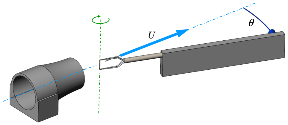
The angular response was measured at a directional calibration facility. Airflow, driven by a blower, passes through a series of screens in a settling chamber before exiting through a nozzle with a diameter of 50 mm. The jet velocity U is controlled by adjusting the blower’s rotational speed. A schematic of the calibration setup is shown in Figure 4. The probe is mounted on a rotating arm that allows the pitch angle $\theta$ to be maintained in the range of ±115°. The axis of rotation (shown as a green dash–dot line) coincides with the sensor axis. Rotation is provided by a stepper motor and controlled by a motor driver National Instruments NI MID-7604 and a labview script running on PC. Inaccuracy in the setting of the angle is estimated to be less than ±0.5°.

Flow velocity is computed from the pressure drop between the inlet and the exit of the nozzle by pressure transmitter Omega PX653-02D5V (Omega Engineering, Inc., Norwalk, CT, USA). Flow temperature measurement is provided by a thermometer Pt100 (Omega Engineering, Inc.) placed in the settling chamber, and data acquisition unit Agilent 34970A (Agilent Technologies, Santa Clara, CA, USA). Barometric pressure is measured by a pressure indicator Druck DPI 145 (Druck Inc., Billerica, MA, USA).

4. Calibration and Decomposition Procedures

The cross-sectional view of the probe (Figure 3) illustrates the arrangement of the two electrically independent film segments separated by a split. The velocity magnitude U and the pitch angle $\theta$ are the quantities we intend to obtain from the measured sensor voltage pair.

4.1. Temperature Correction

The initial step in sensor data processing is a temperature correction to compensate for fluctuations in the fluid temperature. It follows from Equation (1) that the convective heat flux is linearly dependent on the temperature difference between the heated sensor and the surrounding medium. While the CTA system maintains a constant sensor temperature, the fluid temperature may vary during measurement. To address these changes, the measured voltage signal is corrected to the value that would occur at a specific reference fluid temperature ($T_{\mathrm{ref}}$).

While the CTA system maintains a constant sensor temperature, the fluid temperature may vary during measurement. To address these changes, the measured voltage signal is corrected to the value that would be obtained at a specific fluid temperature ($T_{\mathrm{ref}}$) at an identical flow velocity.

The sensor voltage $E_{ai}$ recorded at the actual fluid temperature $T_a$ is converted to the voltage $E_i$ at the reference temperature $T_{\mathrm{ref}}$ using the following relationship [6]:

$$E_i=E_{ai}{\left[{\displaystyle \frac{T_s-T_{\mathrm{ref}}}{T_s-T_a}}\right]}^{1/2}.$$

(4)

The reference temperature $T_{\mathrm{ref}}$ is usually chosen according to calibration conditions.

4.2. Velocity Calibration

Two distinct types of calibration are performed: velocity and angular. During velocity calibration, the relationship between the output voltage $E_i$ and the flow velocity U is determined by holding the probe in a fixed position while varying the flow velocity stepwise.

In thermal anemometry, heat transfer between the heated sensor and the surrounding fluid follows a cooling law [9]. For a given pitch angle $\theta$, the relationship between the sensor-related anemometer output voltage $E_i$, and the flow velocity U, can be described [8] by a modified King’s law:

$$E_{i,\theta }^2=A_i+B_{i,\theta }{U}^{n_{i,\theta }}.$$

(5)

For given fluid properties and sensor overheat are $A_i$, $B_{i,\theta }$ and $n_{i,\theta }$ constants. The constants are determined experimentally from the velocity calibration, where the probe is oriented with respect to the jet by the pitch angle $\theta$. Standard velocity calibration is maintained at zero pitch angle.

The magnitude of velocity of the flow can be found in the same way as for an unsplit film probe. For given flow conditions, total heat flux to the fluid from both sensors is a measure of the velocity. It is widely accepted [6,7,8] that the average output voltage of the two films $E_{12}$ is independent of the pitch angle and follows the cooling law:

$$E_{12}^2=A_{12}+B_{12}{U}^{n_{12}},E_{12}=(E_1+E_2)/2.$$

(6)

The constants $A_{12}$, $B_{12}$ and $n_{12}$ are obtained from a previously performed standard velocity calibration.

4.3. Effective Cooling Velocity

The concept of effective cooling velocity, often employed in thermal anemometry, is adapted in this study specifically for a split-film type of sensor. Here, we assume that the velocity vector lies in the plane normal to the axis of the sensor cylinder. For a split-film sensor, we can define an effective cooling velocity as the velocity at zero pitch angle that would produce the same heat transfer as the actual flow. Sensor voltage $E_i\left(\theta \right)$ recorded at any direction $\theta$ can be converted to effective cooling velocity $U_{Ci}$:

$$U_{Ci}\left(\theta \right)={\left[{\displaystyle \frac{E_i^2\left(\theta \right)-A_i}{B_{i,0}}}\right]}^{1/n_{i,0}}.$$

(7)

It is worth noting that this relation is based on coefficients obtained from the standard velocity calibration.

4.4. Angular Calibration

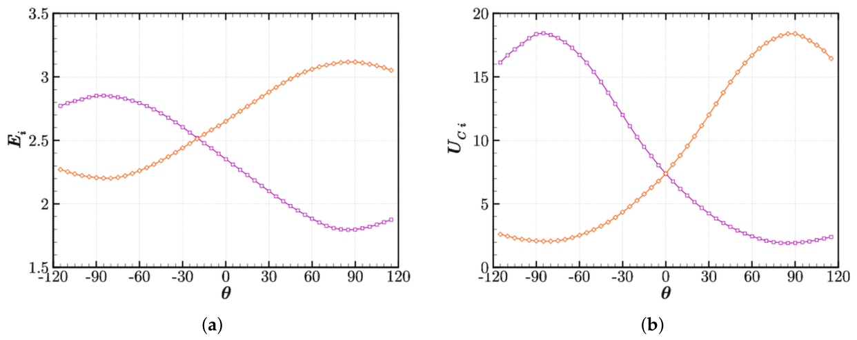
Angular calibration investigates the dependence of the output voltage $E_i$ on the flow direction $\theta$ by incrementally rotating the probe while keeping the flow velocity constant. The angular response of the sensor is shown in Figure 5.

The dependence of the sensor voltage $E_i\left(\theta \right)$ and the corresponding effective cooling velocity $U_{Ci}\left(\theta \right)$ on the flow angle is plotted. For a generally oriented probe, the effective cooling velocities of the two sensors differ. Note that at zero pitch angle, the effective cooling velocities coincide, $U_{C1}\left(0\right)=U_{C2}\left(0\right)$, although the voltages differ, $E_1\left(0\right)\ne E_2\left(0\right)$, due to variations in sensor parameters.

4.5. Decomposition Procedure

The decomposition procedure provides the velocity magnitude and the corresponding flow direction from the measured sensor voltages. The velocity magnitude U is determined from the calibration relation given by Equation (6) in the following form:

$$U={\left[{\displaystyle \frac{E_{12}^2-A_{12}}{B_{12}}}\right]}^{1/n_{12}}.$$

(8)

The flow direction is evaluated through the pitch angle $\theta$ using a dimensionless angle function $Z\left(\theta \right)$ defined in terms of the measured sensor voltages $(E_1,E_2)$:

$$Z\left(\theta \right)=Z(E_1\left(\theta \right),E_2\left(\theta \right)).$$

(9)

The actual pitch angle $\theta$ is then computed from the functional relationship:

$$\theta =f\left(Z\right),$$

(10)

where $f\left(Z\right)$ is obtained from angular calibration.

4.6. Directional Sensitivity

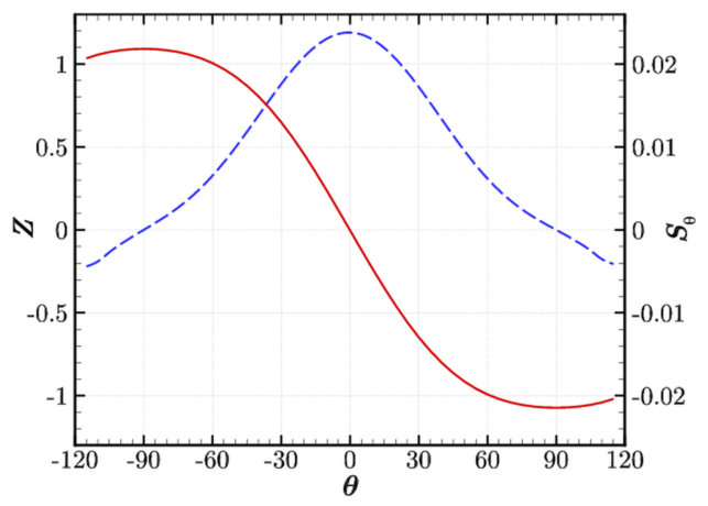
Fundamental behavior of a split-film sensor is demonstrated in Figure 6. Typical angle function Z and directional sensitivity are plotted against the flow angle. The directional sensitivity $S_{\theta }$, defined as the derivative:

$$S_{\theta }={\displaystyle \frac{dZ\left(\theta \right)}{d\theta }},$$

(11)

determines how strongly Z responds to changes in angle $\theta$. It can be seen that the sensitivity is high for small pitch angles. In measurement evaluation, the inverse relationship is used, i.e., the angle $\theta$ is determined from the measured quantity Z by Equation (10). When the sensitivity drops to zero, the angle function becomes locally independent of $\theta$, corresponding to a horizontal tangent of the function $Z\left(\theta \right)$. This lack of directional sensitivity leads to an ill-conditioned sensor behavior.

This limitation is fundamentally physical rather than numerical: in the vicinity of the extrema of the angle function the sensor voltage $E_i$ ceases to respond to changes in the pitch angle. The sensor is incapable of discriminating small changes in flow direction. Consequently, the inverse evaluation function becomes increasingly steep, which drastically amplifies the impact of input errors.

4.7. Accuracy Analysis

The accuracy of flow angle determination is limited by random and systematic errors that occur during calibration and data processing. Random errors are mainly caused by noise in the anemometer signals. This noise introduces uncertainty into the calculated quantities. Systematic errors originate from two main sources: physical and numerical. The physical relationship between sensor output and the pitch angle is altered by the velocity-induced variance in the angular response. Although the proposed method aims to collapse the data onto a single curve, residual velocity-dependent effects remain present. The second source of error is introduced by the numerical model, specifically through the polynomial approximation of the measured behaviour of nominal angle function.

As discussed in the previous section, the accuracy of the method is also affected near pitch angles of ±90° due to poor conditioning. In this region, the directional sensitivity $S_{\theta }$ approaches zero and, as a result, even small signal noise, fitting residuals, and velocity-induced variations are strongly amplified. This amplification leads to large angular estimation errors and thus defines the operational limit of the sensor.

A quantification of each error type is provided in the following sections. The numerical error originating from the regression model is assessed in Section 5.2, while the effect of velocity dependence on the scatter of the angle functions is evaluated in Section 6.4. Finally, the overall accuracy of the proposed methodology is determined in Section 6.5 using the angular estimation error. This error inherently incorporates all previously described sources of uncertainty, including velocity-induced physical variations, random signal noise, and numerical approximation residuals.

5. New Decomposition Method

In the proposed methodology, the angle function is defined using the effective cooling velocity $U_{Ci}$. This approach is analogous to established procedures for X-wire probes, in which the first step consists in converting the recorded sensor voltages into effective cooling velocities. These effective velocities then serve as the primary variables for the subsequent determination of the velocity components and, consequently, the flow direction.

5.1. The Pitch-Angle Function

As a basis for the new angle function, we introduce the function $\zeta \left(\theta \right)$, which is defined directly in terms of the effective cooling velocities:

$$\zeta \left(\theta \right)={\displaystyle \frac{U_{C1}\left(\theta \right)-U_{C2}\left(\theta \right)}{U_{C1}\left(\theta \right)+U_{C2}\left(\theta \right)}}.$$

(12)

As noted earlier, the objective is to define an angle function for which the undesired velocity dependence is minimized. Ideally, for all measurements performed at the same pitch angle, the function would remain constant. In practice, data at a fixed flow angle can be readily obtained during velocity calibration procedure at the reference angle ${\theta }_r$. From such data, the quantity given by Equation (12) is computed and denoted as ${\zeta }_{{\theta }_r}$:

$${\zeta }_{{\theta }_r}={\left.\zeta (\theta ,U)\right|}_{\theta ={\theta }_r}={\zeta }_{{\theta }_r}\left(U\right).$$

(13)

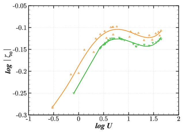
The plot of the logarithm of the absolute value of the quantity ${\zeta }_{{\theta }_r}$ is shown in Figure 7. It reveals that $\zeta$ is not constant, but varies significantly with the velocity magnitude U. This velocity dependence reflects, among other effects, changes in the heat-transfer distribution as the Reynolds number crosses the critical threshold (as discussed in Section 2.3).

Due to the manufacturing imperfections of the probe, the shape of the angular response differs in the negative and positive parts of $\theta$. When performing the reference calibration in each part, deviations caused by asymmetry (geometric and electrical) of the sensor can be partially compensated. For this reason we use two values for reference angle:

$${\theta }_r=\left\{\begin{array}{c}\phantom{-}60°,\phantom{-}0°<\theta <90°\equiv U_{C1}<U_{C2}\equiv \zeta \left(\theta \right)<0\hfill \\ -60°,-90°<\theta <0°\equiv U_{C1}>U_{C2}\equiv \zeta \left(\theta \right)>0\hfill \end{array}\right..$$

(14)

A polynomial regression of logarithms of U and $\left|{\zeta }_{{\theta }_r}\left(U\right)\right|$ is utilized to model the velocity dependence:

$$log\left|{\zeta }_{{\theta }_r}\right|={\displaystyle \sum _{j=0}^m}{d}_{{\theta }_r,j}{log}^{j}U,{\theta }_r=60°,-60°.$$

(15)

Regression using logarithmic variables appears advantageous for describing the behavior in the relatively narrow region near $R{e}_c$. The absolute value of the quantity ${\zeta }_{{\theta }_r}$ is used as the normalization parameter for the angle function.

A new angle function $Z\left(\theta \right)$, based on the function $\zeta \left(\theta \right)$ and normalized using the corresponding reference parameter ${\zeta }_{{\theta }_r}\left(U\right)$, is proposed in the following form:

$$Z\left(\theta \right)={\displaystyle \frac{\zeta \left(\theta \right)}{\left|{\zeta }_{{\theta }_r}\left(U\right)\right|}},{\zeta }_{{\theta }_r}\left(U\right)=\left\{\begin{array}{cc}{\zeta }_{60}\left(U\right)\phantom{0},\hfill & \zeta \left(\theta \right)<0\hfill \\ {\zeta }_{-60}\left(U\right),\hfill & \zeta \left(\theta \right)>0\hfill \end{array}\right..$$

(16)

5.2. Regression Model of the Angular Response

The angular response of the angle function $Z\left(\theta \right)$ is obtained through the angular calibration. In previous works [6,8], the response is described by a polynomial form:

$$\theta =f_b\left(Z\right)\equiv {\displaystyle \sum _{j=0}^m}{b}_j{Z}^j,$$

(17)

where $b_j$ are coefficients determined by a least-squares fit of data. It was found that a polynomial (Equation (17)), even of the fifth degree, is not able to follow the measured data well over the entire range. Improved results are obtained by fitting $sin\theta$ instead:

$$sin\theta =f_c\left(Z\right)\equiv {\displaystyle \sum _{j=0}^m}{c}_j{Z}^j.$$

(18)

The adoption of $sin\theta$ as the dependent variable in the regression model (Equation (18)) is motivated by the close geometric similarity between the angle function’s shape and the trigonometric function. This approach partially linearizes the relationship with the angle function Z and ensures a smooth, monotonic fit across the pitch angle range. The pitch angle is finally computed:

$$\theta =arcsin{\displaystyle \sum _{j=0}^m}{c}_j{Z}^j.$$

(19)

We compared both regression models. Evaluated coefficients are shown in the

Table 2. Polynomial regression coefficients $b_j$ and $c_j$ for the functions $f_b\left(Z\right)$ and $f_c\left(Z\right)$ defined by Equations (17) and (18), respectively.

j	${\mathit{b}}_{\mathit{j}}$	${\mathit{c}}_{\mathit{j}}$
0	$-0.2956$	$-0.0067$
1	$-52.906$	$-0.7564$
2	$-0.2300$	0.0205
3	43.293	0.0244
4	2.3703	$-0.0004$
5	$-52.553$	$-0.1300$

.

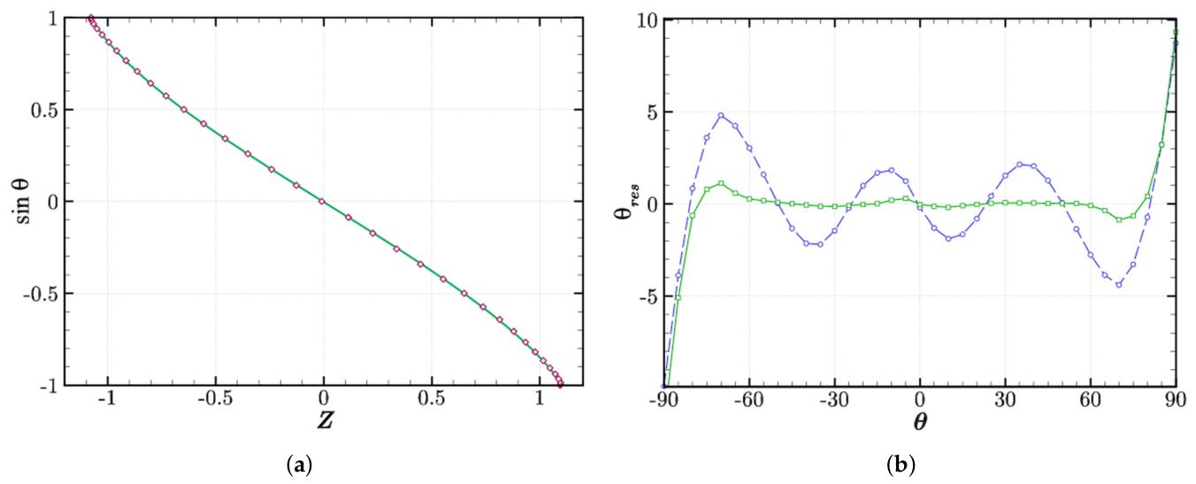
The quality of approximation can be assessed by the fitting residuals. The residuals $y_{\mathrm{res}}$ are the differences between the experimentally measured values y and the values $f\left(x\right)$ prescribed by the polynomial. Maximum residual and standard deviation of residuals, denoted by $y_{\mathrm{res}\max }$ and ${\sigma }_{\mathrm{res}}\left(y\right)$, are defined as

$$y_{\mathrm{res}\max }=\underset{1\le k\le n}{max}\left|y_k-f\left(x_k\right)\right|;{\sigma }_{\mathrm{res}}\left(y\right)={\left[{\displaystyle \frac{1}{n-m+1}}{\displaystyle \sum _{k=1}^n}{\left(y_k-f\left(x_k\right)\right)}^2\right]}^{1/2},$$

(20)

where n is the number of data points and m is the order of the polynomial. Residuals of the pitch angle for both regression models are shown in Figure 8b. The corresponding values of ${\sigma }_{\mathrm{res}}\left(\theta \right)$ and $y_{\mathrm{res}\max }$ are listed in

Table 3. Comparison of models: standard deviation ${\sigma }_{\mathrm{res}}\left(\theta \right)$ [°] and maximum of residuals ${\theta }_{\mathrm{res}\max }$ [°].

Regression Model	$\mathit{\theta }\in [-60°,60°]$		$\mathit{\theta }\in [-80°,80°]$
	${\mathit{\sigma }}_{\mathbf{res}}\left(\mathit{\theta }\right)$	${\mathit{\theta }}_{\mathbf{res}\mathbf{max}}$	${\mathit{\sigma }}_{\mathbf{res}}\left(\mathit{\theta }\right)$	${\mathit{\theta }}_{\mathbf{res}\mathbf{max}}$
$\theta =f_b\left(Z\right)$	1.61	3.03	2.23	4.81
$sin\theta =f_c\left(Z\right)$	0.12	0.29	0.36	1.12

.

The polynomial fit to the measured angular response is shown in Figure 8a.

The oscillatory behavior of the residuals suggests that the traditional model (indicated by circles) is not well suited to accurate representation of the inverse angle function. The plot further shows that the proposed model (indicated by squares) keeps the residuals much closer to zero over most of the angular range. Model performance degrades significantly above 80°. The maximum residual within the pitch-angle interval $[-60°,60°]$ remains below 0.3°, while the standard deviation in this region is an order of magnitude lower than that of the traditional model. Within the applicability range of the method $[-80°,80°]$ the standard deviation remains below 0.4°, with a maximum residual of approximately degradation of the regression model performance.

6. Verification of the Methods

A new form of the angle function $Z\left(\theta \right)$ is compared with two well-established angle-function formulations: the Stock and Jaballa angle function $Z_A\left(\theta \right)$ and the Ahn et al. angle function $Z_B\left(\theta \right)$.

6.1. Existing Forms of Angle Function

In the method by Stock and Jaballa [6] is the angle function $Z_A\left(\theta \right)$ defined:

$$Z_A\left(\theta \right)={\displaystyle \frac{E_1^2\left(\theta \right)-E_{1,0}^2}{E_{1,60}^2-E_{1,0}^2}}+{\displaystyle \frac{E_{2,0}^2-E_2^2\left(\theta \right)}{E_{2,0}^2-E_{2,60}^2}},$$

(21)

where $E_{i,0}$ denotes the reference voltage for velocity U at zero pitch angle, and $E_{i,60}$ corresponds to ${\theta }_r=60°$. The reference voltages are calculated using Equation (5).

The method of Ahn et al. [8] uses the angle function $Z_B\left(\theta \right)$ (denoted as $NZ$ in the original paper):

$$Z_B\left(\theta \right)={\displaystyle \frac{(E_1^2\left(\theta \right)-E_2^2\left(\theta \right))-(A_1-A_2)}{E_{12}^2-A_{12}}},$$

(22)

where all coefficients are known from standard calibration.

6.2. Calibration

First, a standard velocity calibration was performed over a velocity range of 0.5–50 m/s, yielding the constants of the cooling law. The results of the standard calibration are listed in

Table 4. Coefficients of the cooling law of Equations (5) and (8).

i	A	B	n
1	1.0757	1.6096	0.49
2	2.5512	1.6262	0.49
12	1.7010	1.6942	0.49

.

Two additional calibration procedures at reference pitch angles ${\theta }_r=60°$ and −60° were carried out to determine the coefficients of the velocity-dependent parameters. The results are listed in

Table 5. Coefficients $d_j$ of the polynomial fit of Equation (15).

j	${\mathit{d}}_{60,\mathit{j}}$	${\mathit{d}}_{-60,\mathit{j}}$
0	$-0.1875$	$-0.2256$
1	0.1979	0.2481
2	$-0.0543$	$-0.1035$
3	$-0.1318$	$-0.1184$
4	0.0665	0.0685

.

Second, an angular calibration was performed at the nominal velocity $U_n=7.57$ m/s, and the polynomial coefficients $c_j$ were determined using the regression model given in Equation (18). The results are listed in Table 2.

6.3. Test Conditions for Angular Response Comparison

The velocity dependence of both the proposed and existing angle functions was examined through a series of angular response measurements carried out in a directional calibration facility. In total, a set of 24 tests was performed over a velocity range of 2–15 m/s. The flow velocities U and their corresponding Reynolds numbers $Re$, defined by Equation (2) are listed in

Table 6. Summary of experimental conditions for the angular response tests: number of tests, flow velocity U, Reynolds number $Re$, specific marker symbols, and the corresponding line colors used in Figure 9, Figure 10, Figure 11 and Figure 12.

Case	U [m/s]	$\mathit{Re}$	Symbol	Color	Case	U [m/s]	$\mathit{Re}$	Symbol	Color
1	2.23	17.6	△	Green	13	7.57	59.8	◇
2	2.73	21.6			14	7.58	59.9		Violet
3	2.83	22.4			15	8.21	64.8
4	3.26	25.7			16	9.02	71.2	▽
5	3.74	29.5			17	9.83	77.6
6	4.17	32.9			18	10.61	83.8		Magenta
7	4.64	36.6			19	11.20	88.5
8	5.14	40.6	◯	Orange	20	11.79	93.1
9	5.62	44.4			21	12.55	99.1		Blue
10	6.25	49.4			22	13.13	103.7
11	6.66	52.6			23	13.89	109.7
12	6.95	54.9			24	14.63	115.6	☐

. The table serves as the primary legend for interpreting the presented experimental results.

Graphs in Figure 9, Figure 10, Figure 11 and Figure 12 illustrate how the velocity magnitude influences the directional response and the accuracy of different calibration methods. During both the calibration and the validation tests, the fluid temperature varied from 20.4 °C to 22.1 °C. The reference temperature for the signal correction (Equation (4)) was $T_{\mathrm{ref}}=21.0$ °C.

6.4. Deviation of Angle Functions

The method employs a polynomial approximation of the nominal angle function for evaluating the flow angle from the sensor signals. The primary objective of this study is to reduce velocity-induced variations in the shape of the angle curve. Ideally, the data for any flow velocity should collapse onto a single universal curve. The nominal angle curve, denoted as $Z_n\left(\theta \right)$, is determined from the angular calibration at the nominal velocity $U_n$:

$$Z_n\left(\theta \right)={\left.Z\left(\theta \right)\right|}_{U=U_n}.$$

(23)

From this calibration, the regression coefficients $c_j$ (see Equation (18)) are obtained. Since the compensation is not perfect, deviations from the nominal curve are observed. To evaluate the deviation of the actual angle function from the nominal curve, the value of $Z_n$ must be computed for a given angle $\theta$:

$$Z_n=f_c^{-1}(sin\theta );sin\theta =f_c\left(Z_n\right)\equiv {\displaystyle \sum _{j=0}^m}{c}_j{Z}_n^j.$$

(24)

To avoid additional errors that would arise from introducing a further approximation of the $f_c^{-1}$ function, the values of $Z_n$ are computed numerically from the previously determined coefficients $c_j$ using an iterative procedure. The normalized curve deviation is then defined as the difference between the measured and nominal curves, normalized by the value of the nominal curve at $\theta =90°$:

$$\Delta Z^{*}\left(\theta \right)={\displaystyle \frac{Z\left(\theta \right)-Z_n\left(\theta \right)}{\left|Z_n(90°)\right|}}.$$

(25)

For an overall assessment of the velocity compensation performance, the maximum, $\Delta Z_{max}$, and the standard deviation, $\sigma (\Delta Z)$, of the normalized curve deviation are evaluated:

$$\Delta Z_{max}^{*}=\underset{1\le k\le n}{max}|\Delta Z_k^{*}|;\sigma (\Delta Z^{*})={\left[{\displaystyle \frac{1}{n}}{\displaystyle \sum _{k=1}^n}{(\Delta Z_k^{*}-\overline{\Delta Z^{*}})}^2\right]}^{1/2}.$$

(26)

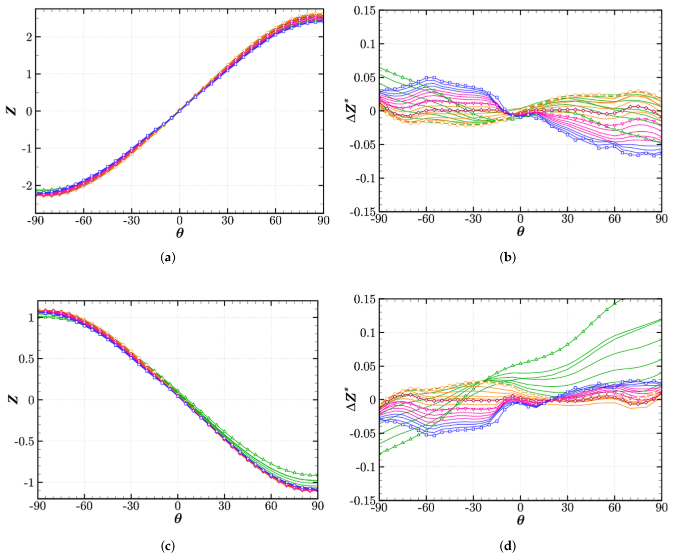
The following graphs show an angle function $Z\left(\theta \right)$ computed from angular test at each velocity. On the right-hand side, the deviation $\Delta Z^{*}\left(\theta \right)$ is shown.

The graphs in Figure 9 illustrate the limitations of conventional methods when applied to a wide velocity range. The plots reveal a notable velocity-induced deviation from the nominal curve, with maximum discrepancies ranging from 0.06 to 0.18.

Figure 9. Existing angle functions Z [-] and their deviation from nominal function $\Delta Z^{*}$ [-] versus pitch angle $\theta$ [°]. Angle function of Stock and Jaballa [6]: $Z_A\left(\theta \right)$ (a), $\Delta Z_A^{*}\left(\theta \right)$ (b) and Ahn et al. [8]: $Z_B\left(\theta \right)$ (c), $\Delta Z_B^{*}\left(\theta \right)$ (d).

Figure 9. Existing angle functions Z [-] and their deviation from nominal function $\Delta Z^{*}$ [-] versus pitch angle $\theta$ [°]. Angle function of Stock and Jaballa [6]: $Z_A\left(\theta \right)$ (a), $\Delta Z_A^{*}\left(\theta \right)$ (b) and Ahn et al. [8]: $Z_B\left(\theta \right)$ (c), $\Delta Z_B^{*}\left(\theta \right)$ (d).

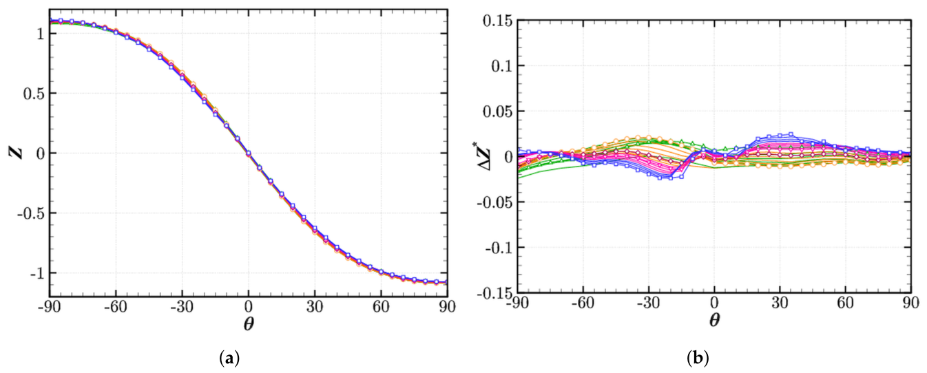
In contrast to traditional models, the proposed angle function $Z\left(\theta \right)$ achieves a remarkable collapse of data points for the entire range of velocities examined (Figure 10). The corresponding deviation plot shows that the normalized error is significantly reduced, confirming that the new normalization effectively reduces the velocity-dependent effects. A comparison of the results is presented in

Table 7. Comparison of methods: standard deviation $\sigma (\Delta Z^{*})$ [%] and the maximum deviation $\Delta Z_{max}^{*}$ [%].

Method	$\mathit{\theta }\in [-90°,90°]$
	$\mathit{\sigma }(\mathbf{\Delta }{\mathit{Z}}^{\mathbf{*}})$	$\mathbf{\Delta }{\mathit{Z}}_{\mathbf{max}}^{\mathbf{*}}$
Stock and Jaballa [6]	3.08	6.94
Ahn et al. [8]	4.21	18.24
Present study	0.84	2.45

.

Figure 10. Proposed angle function Z [-] (a) and its deviation from the nominal function $\Delta Z^{*}$ [-] versus pitch angle $\theta$ [°] (b).

Figure 10. Proposed angle function Z [-] (a) and its deviation from the nominal function $\Delta Z^{*}$ [-] versus pitch angle $\theta$ [°] (b).

An analysis of the directional response definitions reveals a compromise between implementation simplicity and physical accuracy. The formulation by Ahn et al. (Equation (22)) is the simplest to apply, as it does not require a reference calibrations for inclined flow conditions.

However, it yields the least accurate results, especially at high pitch angles, because it fails to account for the changes in heat transfer distribution during asymmetrical cooling. The Stock and Jaballa method (Equation (21)) improves precision by requiring additional reference calibration.

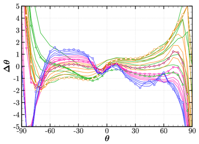
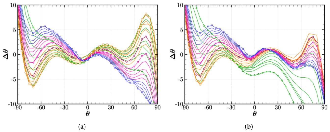
Figure 11. Angular estimation error $\Delta \theta$ [°] as a function of pitch angle $\theta$ [°] for the methods of Stock and Jaballa (1985) $\Delta {\theta }_A$ (a) and Ahn et al. (1995) $\Delta {\theta }_B$ (b).

Figure 11. Angular estimation error $\Delta \theta$ [°] as a function of pitch angle $\theta$ [°] for the methods of Stock and Jaballa (1985) $\Delta {\theta }_A$ (a) and Ahn et al. (1995) $\Delta {\theta }_B$ (b).

The newly proposed definition (Equation (16)) uses two reference calibrations and provides the most effective compensation of the angle function. This is achieved by explicitly compensating for the velocity dependence of the directional response through velocity-dependent reference parameters, an effect not considered in the approach of Ahn et al.

Figure 12. Angular estimation error $\Delta \theta$ [°] as a function of pitch angle $\theta$ [°] of the proposed method.

Figure 12. Angular estimation error $\Delta \theta$ [°] as a function of pitch angle $\theta$ [°] of the proposed method.

6.5. Angular Estimation Error

The angle functions were finally validated through a reverse calibration experiment. For known values of the velocity magnitude, the pitch angle was varied and the corresponding anemometer output signals were recorded. The recorded signals were then used to compute the pitch angle.

Angular estimation error $\Delta \theta$ is defined as a difference angle between the value computed by the method $\theta$ and the one set on calibration facility ${\theta }_t$:

$$\Delta \theta =\theta -{\theta }_t.$$

(27)

For given range of angles $\theta$, the maximum angular error, $\Delta {\theta }_{max}$, and the standard deviation of the angular error, $\sigma (\Delta \theta )$, are used to evaluate the overall accuracy of the model:

$$\Delta {\theta }_{max}=\underset{1\le k\le n}{max}|\Delta {\theta }_k|;\sigma (\Delta \theta )={\left[{\displaystyle \frac{1}{n}}{\displaystyle \sum _{k=1}^n}{(\Delta {\theta }_k-\overline{\Delta \theta })}^2\right]}^{1/2}.$$

(28)

As discussed above, the angular error estimation inherently reflects the combined impact of all error sources, ranging from physical velocity-induced variance to random noise and numerical fitting residuals.

The accuracy assessment of established methods in Figure 11 reveals substantial errors in flow direction determination, particularly at high pitch angles and low velocities. Discrepancies frequently exceed ±5° for pitch angle $\theta =60°$.

The results of the angular estimation error, displayed in Figure 12, show that the newly proposed methodology maintains the total error $\Delta \theta$ mostly below ±2° over the pitch angle interval $[-60°,60°]$. Note the reduced y-axis scale compared to Figure 11, which reflects the lower error level. Over the wider pitch angle interval $[-70°,70°]$, the total error remains within ±3°. The obtained results are summarized in

Table 8. Comparison of methods: standard deviation $\sigma (\Delta \theta )$ [°] and the maximum value $\Delta {\theta }_{max}$ [°] of the angular estimation error.

Method	$\mathit{\theta }\in [-60°,60°]$		$\mathit{\theta }\in [-70°,70°]$		$\mathit{\theta }\in [-80°,80°]$
	$\mathit{\sigma }(\mathbf{\Delta }\mathit{\theta })$	$\mathbf{\Delta }{\mathit{\theta }}_{\mathbf{max}}$	$\mathit{\sigma }(\mathbf{\Delta }\mathit{\theta })$	$\mathbf{\Delta }{\mathit{\theta }}_{\mathbf{max}}$	$\mathit{\sigma }(\mathbf{\Delta }\mathit{\theta })$	$\mathbf{\Delta }{\mathit{\theta }}_{\mathbf{max}}$
Stock and Jaballa [6]	1.94	5.77	2.36	7.64	2.81	10.28
Ahn et al. [8]	2.39	13.11	2.67	17.18	3.20	23.09
Present study	0.70	1.83	0.83	2.87	1.26	6.38

.

The effective collapse of the curves achieved by the proposed normalization represents the scientific advance of this study, as it successfully suppresses velocity-induced variations in the directional response. The framework provides a robust and stable alternative for precise measurements in complex flow environments characterized by high unsteadiness or low-velocity regimes. Since the laboratory verification was successful, the proposed methodology shows strong potential for industrial and field applications, particularly due to its experimental simplicity and non-iterative nature.

During the calibration of the probe velocity, it is recommended to cover the entire range of expected velocities and to avoid extrapolation both when determining the coefficients of the cooling law and when fitting the polynomial describing the velocity dependence of the normalization parameter.

7. Conclusions

The study focuses on the directional behavior of a split-film probe over a velocity range of 2–15 m/s. Within this range, two existing decomposition methods were evaluated. Both conventional methods exhibit a notable velocity-induced variance in their angle functions, which manifests as significant data scatter. A novel decomposition method was therefore proposed to improve pitch angle determination over a wide range of flow velocities.

A significant effort to reduce velocity dependence was previously undertaken by Ra et al., who proposed decoupling the velocity function from the directional response. A notable disadvantage of their approach is the requirement for a more extensive set of calibration data across the entire operating range to characterize the separated velocity and angular functions. Furthermore, obtaining the required functions in their model necessitates an impractical iterative procedure. In contrast, the present methodology offers a substantial practical advantage, as all polynomial coefficients are determined directly from calibration data.

The proposed methodology employs an enhanced regression model for the angular response. The use of $sin\theta$ as the dependent variable in the regression model yields a significantly lower standard deviation of residuals compared to traditional polynomial models, achieving a nearly fourfold reduction in fitting error. This approach, which uses the the geometric similarity between the angle function and trigonometric functions, ensures a smooth and monotonic fit. The applicability of the method is limited near the extrema of the angle function (approximately $\pm 90°$) due to vanishing directional sensitivity, loss of validity of the regression model, and residual velocity dependence. The method remains stable within a pitch angle range of $[-80°,80°]$. Furthermore, because it effectively suppresses the velocity dependence of the directional function, the method maintains a pitch angle error typically within ±2° in the interval $[-60°,60°]$, whereas conventional methods under similar conditions often exceed ±5.5°.

In conclusion, the proposed methodology is experimentally straightforward, as it requires only one standard velocity calibration, one angular calibration, and supplementary measurements of the velocity dependence parameters at two specific pitch angles, following a procedure equivalent to conventional velocity calibration. It offers a substantial improvement for measurements in complex flow environments characterized by low velocities, such as wakes behind bluff bodies or near-wall separated regions. This significantly extends the reliable operating range of split-film probes in highly unsteady, low-speed flow fields.