Abstract
Hydrogen energy is valued for its diverse sources and clean, low-carbon nature and is a promising secondary energy source with wide-ranging applications and a significant role in the global energy transition. Nonetheless, hydrogen’s low energy density makes its large-scale storage and transport challenging. Liquid hydrogen, with its high energy density and easier transport, offers a practical solution. This study examines the global hydrogen liquefaction methods, with a particular emphasis on the liquid nitrogen pre-cooling Claude cycle process. It also examines the factors in the helium refrigeration cycle—such as the helium compressor inlet temperature, outlet pressure, and mass—that affect energy consumption in this process. Using HYSYS software, the hydrogen liquefaction process is simulated, and a complete process system is developed. Based on theoretical principles, this study explores the pre-cooling, refrigeration, and normal-to-secondary hydrogen conversion processes. By calculating and analyzing the process’s energy consumption, an optimized flow scheme for hydrogen liquefaction is proposed to reduce the total power used by energy equipment. The study shows that the hydrogen mass flow rate and key helium cycle parameters—like the compressor inlet temperature, outlet pressure, and flow rate—mainly affect energy consumption. By optimizing these parameters, notable decreases in both the total and specific energy consumption were attained. The total energy consumption dropped by 7.266% from the initial 714.3 kW, and the specific energy consumption was reduced by 11.94% from 11.338 kWh/kg.
1. Introduction
1.1. Global Developments in Hydrogen Energy
Hydrogen is being more widely recognized as a crucial component in the transition to a sustainable energy future, with numerous countries developing national hydrogen strategies [1]. The global hydrogen demand reached a record high in 2023 (up 2.5% from 2022) and is expected to continue growing in the coming years [2]. By mid-century, hydrogen could meet an estimated 18% of the world’s total energy demand, helping to prevent about 6 Gt of CO2 emissions annually. Projections predict that by 2050, China’s hydrogen demand will be nearly 60 million tons annually, accounting for over 10% of its end-use energy and potentially reducing CO2 emissions by about 700 million tons. This global and national momentum highlights hydrogen’s broad potential to decarbonize hard-to-abate sectors (e.g., heavy transport and industry) and to store and distribute renewable energy at scale [1].
However, realizing a “hydrogen economy” will require building a substantial hydrogen value chain, including large-scale transport and storage infrastructure. Unlike fossil fuels, hydrogen has a very low energy density at ambient conditions (~3 Wh/L) [3] making its distribution challenging. Pipeline networks for hydrogen remain limited (for example, the U.S. has ~2600 km of H2 pipelines and the EU has ~2000 km, whereas China only has ~100 km according to a 2024 report by MacroPolo). Transporting hydrogen over long distances or in bulk will therefore likely rely on liquid hydrogen (LH2), which has a drastically higher energy density. Indeed, liquefaction and intermediate cryogenic storage are expected to play a crucial role in future international hydrogen trade and long-distance delivery systems. In this context, the development of efficient hydrogen liquefaction technology and infrastructure has become a critical enabling step in the global hydrogen supply chain.
1.2. Hydrogen Liquefaction Technology
The process of liquefying hydrogen is crucial for developing hydrogen liquefaction systems. In 1898, James Dewar achieved this by cooling hydrogen after pressurizing it to 20 megapascals and then throttling it. As modern technology has advanced, hydrogen liquefaction technology has evolved into various processes. Currently, three processes are primarily employed: the Linde–Hampson (L-H) cycle, helium expansion refrigeration, and hydrogen expansion refrigeration. Recently, several new hydrogen liquefaction methods have been developed that effectively decrease the energy use of hydrogen liquefaction. Micro-liquefaction units with G-M-type gas reheat cryocoolers are mainly used as cold sources, but not for large-scale hydrogen storage and transport. Hydrogen liquefaction efficiency impacts the overall energy use. Traditional hydrogen liquefaction involves nitrogen pre-cooling, hydrogen pressurization, and expansion refrigeration. This is followed by helium expansion refrigeration, which results in a relatively high energy consumption. Table 1 compares various hydrogen liquefaction processes.

Table 1.
Various hydrogen liquefaction processes. (Note: Data summarized from multiple sources including [4,5].)
The Linde–Hampson cycle, developed in the late 1800s by Carl von Linde and William Hampson, is a basic method for gas liquefaction that is mainly suitable for gases like nitrogen that can expand and cool at ambient temperatures. Due to the high theoretical specific work required for liquefaction, which was calculated to be as high as 68.10 kWh/kg, it is currently virtually unused. The Joule–Thomson refrigeration cycle, also called the throttling cycle, uses the Joule–Thomson effect to cool high-pressure gas through a throttle valve. The resulting product is transferred to the feed gas via a heat exchanger to achieve liquefaction. Since the Joule–Thomson coefficient of some gases is negative at high temperatures, the gas must be pre-cooled to enable effective throttling and cooling. This cycle has a simple structure and low equipment investment but low efficiency, making it suitable for small to medium-sized liquefaction units. In contrast, the Joule–Thomson + expansion refrigeration cycle, also known as the Claude cycle, adds an expansion machine to the throttling cycle. Part of the gas undergoes adiabatic expansion in an expansion machine to generate additional cooling capacity, thereby improving the cycle efficiency and reducing the energy consumption. This cycle fully utilizes both throttling and expansion cooling mechanisms and is the mainstream process for large-scale liquefaction units. Since the single-pressure Claude cycle has a specific energy consumption of about 22.1 kWh/kg using liquid nitrogen pre-cooling [4], Baker [5] proposed a two-pressure process that reduces the energy required for hydrogen liquefaction. The theoretical demand is 10.85 kWh/kg for large plants.
Currently, in practical applications, the energy consumption of the two-stage Claude cycle remains relatively high, typically exceeding 10 kWh/kg. To decrease the energy use in hydrogen liquefaction, new process configurations were developed recently, such as mixed working fluid pre-cooling, J-B (Joule–Brayton) cycles, and LNG pre-cooling technologies. The traditional isothermal cold sources used for pre-cooling cause large temperature differences between hot and cold fluids, leading to energy losses. Therefore, developing new pre-cooling methods, such as mixed working fluids, is crucial in order to better match temperatures and lower energy use.
Quack [6] et al. introduced a Joule–Brayton (J-B) pre-cooled Claude cycle using propane, with helium–neon as the refrigerant in the low-temperature stage. Its specific energy consumption varies with product needs and feed gas conditions, usually staying below 5–7 kWh per kg of LH2. Kuz’menko et al. [7] designed a process utilizing nitrogen pre-cooling and helium refrigeration, which exhibits high safety and pollution-free characteristics. Stang et al. [8] conducted simulations based on data from the Ingolstadt liquefaction plant in Germany and designed an experimental hydrogen liquefaction facility using MR system pre-cooling. They reported that the current industrial energy consumption is in the range of 11.9–13.6 kWh/kg LH2, and through MR pre-cooling designs, they achieved simulations yielding 6.15–6.48 kWh/kg LH2. Valenti et al. [9] proposed a hydrogen liquefier employing four helium Joule–Brayton cycles for cooling, achieving a capacity of 10 kg/s with an efficiency of approximately 48%. Asadnia et al. [10] designed a process capable of producing 100 tons per day. The process begins by pre-cooling hydrogen to −198.2 °C using an MR cycle and a hydrogen expansion refrigeration cycle. It then cools the hydrogen further to −251.8 °C via six Joule–Brayton cascade refrigeration cycles. The process consumes 7.69 kWh per kilogram of liquid hydrogen and operates at an efficiency of 39.5%. Sadaghiani, Mehrpooya, et al. [11] examined the effectiveness of different mixed refrigerants in low-temperature hydrogen liquefaction, achieving an efficiency of up to 55.47%. Yin, Ju, et al. [12] employed Aspen HYSYS software to simulate and improve a hydrogen liquefaction system that uses liquid nitrogen pre-cooling and helium expansion refrigeration. They utilized a genetic algorithm to optimize the system parameters, resulting in a reduction in energy use to 7.13 kWh/kg LH2 and achieving an efficiency of 49.41%. Amjad et al. [13] designed a process that employs a mixed-fluid cascade model using Aspen HYSYS. They utilized the cooling energy from LNG during the hydrogen pre-cooling stage, which markedly decreased the total refrigerant needed, cut the cooling requirement by approximately 50%, and reduced the specific energy use to 7.64 kWh per kg of LH2. The process achieved an efficiency of 42.25%. Naquash et al. [14] used three MR cycles and one CO2 cycle and achieved an energy consumption of 7.63 kWh/kg and efficiency of 31.4%. Wang Guocong et al. [15] enhanced the MR refrigeration cycle with a genetic algorithm, achieving a 24.07% decrease in specific energy use. Wang Chao et al. [16] used a particle swarm optimization algorithm to improve the MR pre-cooling process, lowering the specific energy consumption to 6.98 kWh/kg LH2 after optimization. Xu et al. [17] proposed an integrated hydrogen and LNG production process using industrial by-product gases as feedstock and employing a two-stage helium reverse Brayton cycle. Bi et al. [18] optimized a novel hydrogen liquefaction process using circulating hydrogen refrigeration and demonstrated improved energy efficiency. Naquash et al. [18] improved hydrogen liquefaction efficiency by combining absorption refrigeration with an ORC-driven liquid air energy system. Zhang and Liu [19] designed and performed an in-depth analysis of a hydrogen liquefaction process, evaluating its energy efficiency, environmental effects, and economic feasibility across various setups.
Table 2 presents the key performance indicators for hydrogen liquefaction cycles, which measure energy use, efficiency, and yield, to compare process schemes.
Table 2.
Key indicators of liquefaction cycles.
Currently, many new hydrogen liquefaction processes remain in the theoretical research stage and have not yet been widely adopted in actual production. These processes are typically complex and involve significant equipment investment costs. For example, the typical J-B process employs a mixed working fluid pre-cooling cycle, primarily drawing on MRC technology from the large-scale natural gas liquefaction industry [20], which requires the use of multi-stage oil-free compressors and other high-end equipment, significantly increasing the overall costs. Compared to liquid nitrogen pre-cooling, these technologies may not offer obvious cost advantages, thereby limiting their application in commercial settings. On the other hand, liquid two-phase low-temperature expansion machines and low-temperature compressor technologies are still immature, and some new processes require these technologies, making it difficult to implement these processes in practice. Table 3 presents a comparison of various simple basic hydrogen liquefaction processes.
Table 3.
Comparison of simple basic hydrogen liquefaction cycles. (Note: Data summarized from multiple sources including [1,3,5,21].)
1.3. Global Liquid Hydrogen Plant Projects
Recently, the United States, the Republic of Korea, and China have been actively developing liquid hydrogen facilities and growing their hydrogen energy infrastructure. For example, Air Products’ liquid hydrogen plant in La Porte, Texas, began operation in October 2021, producing roughly 30 tons daily [22]. The company is also developing China’s first large-scale commercial liquid hydrogen plant in Haiyan, Zhejiang Province, with a planned daily capacity of 30 tons [23]. Originally set to begin operations in 2022, it will be Asia’s first liquid hydrogen plant of this magnitude. Plug Power launched the largest electrolyzed hydrogen plant in the United States in early 2024 in Georgia, with a daily capacity of around 15 tons, supported by PEM electrolyzers and cryogenic liquefaction for uses like hydrogen-powered forklifts [24]. The Republic of Korea’s first commercial liquid hydrogen plant, built by Doosan Enerbility, was finished in August 2023 and started operations in early 2024, with a daily output of about 5 tons [25]. The project is backed by local government funding for developing a hydrogen refueling station network. Additionally, the Republic of Korea plans to construct a liquid hydrogen plant in Ulsan in collaboration with Hyosung Group and Linde (with a planned daily production of approximately 36 tons) and an Incheon project (with a planned daily production of approximately 82 tons). Hydrogen liquefaction facilities are located in countries including the United States, Canada, Japan, and China. Air Products, established in 1942 and headquartered in the United States, provides more than half of the hydrogen liquefaction units in the country, but it has not yet entered the Chinese market. Meanwhile, Plug Power, a provider of hydrogen energy solutions, is actively expanding its involvement in the hydrogen liquefaction industry.
The originality of this work is that it systematically analyzed the thermodynamic and process parameters affecting the specific energy consumption for hydrogen liquefaction in a pre-cooled Claude cycle. Previous works often focused on modifications to the process in the context of the optimization of a single parameter or they performed a sensitivity analysis across multiple parameters. In this work, we combined steady-state optimization with a multi-parameter sensitivity analysis to identify the most important operational variables. The results provide useful guidance for the range of parameters that leads to an energy-efficient design under a specific operating constraint.
2. Simulation Tools and Process Design
The simulation software used in this study, Aspen HYSYS v14, is a comprehensive and powerful process simulation software developed by Aspen Tech, Inc., in Bedford, MA, USA. HYSYS provides a wealth of physical property data, dynamic simulation capabilities, energy analysis tools, safety system designs, and control system design functionalities.
2.1. Ortho- and Para-Hydrogen Properties
Diatomic hydrogen has two spin isomers: ortho-hydrogen (parallel proton spins) and para-hydrogen (antiparallel spins). They differ in energy and properties, with ortho-hydrogen having a higher energy and is more abundant at room temperature. At low temperatures, ortho-hydrogen converts to para-hydrogen, releasing heat. It is important to consider these spin isomers when handling liquid hydrogen.
Under ideal conditions, the oxygen concentration during liquefaction is balanced, releasing conversion heat at the highest temperature. However, integrating a catalytic bed and heat exchanger is relatively challenging. In modern hydrogen liquefaction technology, to enhance efficiency and optimize energy consumption, most hydrogen liquefaction units employ multi-stage conversion processes to approximate a continuous conversion process. In these processes, hydrogen gas or liquid hydrogen undergoes catalytic conversion through a bed of solid catalyst. The catalytic conversion reactions can generally be classified into the following three categories.
- (1)
- Isothermal reaction: In this process, no external cooling source is used; instead, the heat produced by the reaction itself raises the temperature of the hydrogen gas. To effectively manage the heat generated in this scenario, a multi-stage temperature control approach is typically employed, using multiple isothermal conversion beds to gradually remove heat and maintain thermal equilibrium in the system.
- (2)
- Isothermal reactions: These reactions occur in fine tubes or channels filled with catalyst, using liquid nitrogen or liquid hydrogen for external cooling to maintain a constant temperature during the reaction process. Although this method has a relatively high energy consumption, its reactor design is simple, its operation is convenient, and it requires less catalyst, making it suitable for applications requiring precise temperature control.
- (3)
- Continuous reaction: In this mode, the heat exchanger channels are filled with the catalyst to achieve continuous cooling and conversion of the feed gas. Although this method has the lowest energy consumption, it is structurally complex, requires a large amount of catalyst, and has high flow resistance, making the design and maintenance of the systems using this method more complicated. In fact, an integrated catalyst heat exchanger has been developed and tested, and this design has been applied in hydrogen liquefaction facilities in Ontario and California, and its effectiveness in achieving near-ideal continuous conversion processes has been demonstrated.
Common measures to speed up the conversion of para-hydrogen during hydrogen liquefaction include using catalysts (such as iron hydroxide and chromium oxide), which reduce the need for boiling during storage.
However, Aspen HYSYS does not include a dedicated ortho–para conversion module. In this study, the conversion process was modeled using a heat exchanger and a heater to account for the enthalpy change associated with ortho–para conversion, without explicitly simulating the catalytic kinetics. This steady-state thermodynamic approach has been adopted in previous modeling studies [26]. Since catalyst kinetics were not explicitly modeled, the results do not capture the transient behavior of ortho–para conversion. However, for steady-state energy analysis, this simplification has negligible influence on the overall specific energy consumption trends.
2.2. Purification of Hydrogen Feed Gas
The sources of raw hydrogen are diverse, including water electrolysis, catalytic cracking of ammonia or methanol, synthesis gas from ammonia production, natural gas reforming, refinery off-gas, coke oven gas, and chemical process off-gas. The hydrogen supplied from these sources varies significantly in hydrogen content and impurity levels. For example, the hydrogen gas volume fraction obtained from synthetic ammonia feed gas is typically around 70%, but it also contains a significant amount of nitrogen and carbon monoxide. Hydrogen produced via natural gas reforming can achieve a volume fraction of 95%, though it also contains methane and carbon monoxide. Hydrogen generated through water electrolysis is relatively pure but may still contain trace amounts of nitrogen and oxygen impurities. These impurities can have adverse effects on catalysts, such as reducing the catalyst efficiency, causing incomplete conversion, or leading to blockage of conversion pathways. In particular, hydrogen with a high oxygen content may form solid oxygen at lower temperatures, and accumulated solid oxygen could trigger explosions. Therefore, thorough purification treatment before hydrogen enters the conversion or liquefaction stage is critical.
In the Leuna and IDEALHY hydrogen liquefaction projects, purifiers are used to improve the hydrogen purity, which differs from the Ingolstadt plant. In the Leuna and IDEALHY projects, purification happens in the pre-cooling heat exchanger instead of an independent nitrogen bath. This study assumed that the feed hydrogen is already purified to 99.9999%, which is crucial for process efficiency and safety.
2.3. Pre-Cooling Methods
During gas liquefaction, adding more pre-cooling stages usually lowers the total energy use. However, this approach also increases equipment complexity and raises operational and maintenance costs. Therefore, it is essential to strike a balance between improving efficiency and controlling costs, and to select the appropriate number of pre-cooling stages. Typically, in lower conventional temperature zones, pre-cooling agents such as liquid ammonia or propane can reduce the temperature to 238–248 K. In lower temperature ranges, whether at atmospheric pressure or reduced pressure, liquid nitrogen is a commonly used pre-cooling agent; it is capable of lowering the hydrogen temperature to 65–80 K. In ammonia synthesis plants, liquid ammonia is frequently used as a pre-cooling agent due to its availability and ability to reduce the temperature to 223–233 K. However, some facilities producing liquid ammonia may opt for fluorocarbons, which pose greater potential environmental hazards and have higher costs. Additionally, within the temperature range for liquid ammonia and liquid nitrogen to exist, liquefied natural gas (LNG) can also be used as a pre-coolant to further reduce the hydrogen temperature to 110 to 120 K. Due to methane’s significant Joule–Thomson (JT) effect during throttling expansion, its efficiency is two to three times higher than that of other gases, making LNG the preferred pre-coolant. However, since liquid hydrogen production facilities typically do not produce LNG, its use is limited.
Considering that liquid nitrogen is relatively easy to obtain, as it can be produced by repeatedly compressing and throttling air to obtain liquid air, followed by separation to obtain liquid nitrogen, and has lower costs, this study selected a liquid nitrogen system for pre-cooling. This method reduces the hydrogen temperature and supports economic and environmental sustainability.
2.4. Refrigeration Methods
When designing small-scale hydrogen liquefaction equipment, priority should be given to simple refrigeration processes to ensure stable operation while also considering energy consumption. When designing large-scale hydrogen liquefaction plants, it is crucial to aim for low energy consumption, minimal investment costs, and operational safety and reliability.
- (1)
- Helium Expansion Refrigeration
The helium expansion refrigeration process typically begins with liquid nitrogen pre-cooling, followed by further cooling of the raw hydrogen gas through a multi-stage helium expansion heat exchanger. Concurrently, catalytic conversion of normal hydrogen to deuterated hydrogen is performed to enhance the liquefaction efficiency. Helium is recycled through multiple heat exchangers and undergoes expansion, compression, and cooling to maintain the system’s low temperature. As an inert gas, helium is safe, remains gaseous at all times, has a simple design, and can achieve high efficiency, making it suitable for liquid hydrogen production units with a daily output of less than 3 tons. This study selected helium expansion refrigeration as the primary cooling strategy.
- (2)
- Hydrogen expansion refrigeration
Hydrogen expansion refrigeration is divided into two types: an independent hydrogen cycle and split hydrogen cycle. In the independent cycle, hydrogen is compressed, water-cooled, and pre-cooled with liquid nitrogen before expanding to allow it to cool down, with part of the cooled hydrogen being recycled. The Japanese WE-NET project employs this process, combining cooling and expansion refrigeration into two steps, with liquid hydrogen ultimately stored stably at 20.4 K and 106 kPa. In the split-flow cycle, hydrogen gas is compressed, pre-cooled with liquid nitrogen, and divided into two streams. One stream expands to cool and form the cold stream, while the other undergoes heat exchange in a heat exchanger and undergoes normal-para conversion. The U.S. company Praxair adopts this method, achieving efficient and safe liquefaction through precise thermal management and split control.
- (3)
- Hydrogen throttling expansion
When hydrogen undergoes expansion via a throttle valve, cooling is achieved through the Joule–Thomson (J–T) effect. This phenomenon produces a temperature variation in real gases during isenthalpic throttling, which is driven by intermolecular forces. It is a widely employed cooling method in gas liquefaction processes.
2.5. Equations of State
In Aspen Plus software v14, users can select from a variety of cubic state equations, including options based on SRK (Soave–Redlich–Kwong) such as RK-SOAVE, RK-ASPEN, RKSMHV2, and RKSWS, as well as options based on PR (Peng–Robinson) such as Peng–Robinson, PRMHV2, and PRWS. The Peng–Robinson state equation is particularly suitable for mixtures containing non-polar and weakly polar components with light gases, and demonstrates superior performance in terms of computational accuracy. This makes it particularly suitable for simulating hydrogen liquefaction processes, enabling the accurate prediction of thermodynamic properties involving light components such as hydrogen, thereby optimizing the design and operation of these processes.
In hydrogen liquefaction processes, particularly when no complex chemical reactions are involved and the primary goal is to liquefy gases, the Peng–Robinson equation provides a reliable basis for property calculations. The specific form of this equation is as follows:
In this equation, p is the pressure, T is the temperature, V is the molar volume, R is the gas constant, and a and b are substance-specific parameters that account for intermolecular attraction and molecular volume, respectively.
The Peng–Robinson equation of state (PR EOS) was chosen for the thermodynamic property calculations in Aspen HYSYS. Along with its quick computation, PR EOS is a widely accepted approach for cryogenic hydrogen systems and has good accuracy. Several researchers have shown that PR EOS can accurately predict vapor–liquid equilibrium and thermophysical properties of hydrogen over a wide range of temperatures, including regions close to the normal boiling point of hydrogen [27]. The predictions for liquid density from PR EOS are often better than other cubic equations of state, which is especially important in the calculations for specific energy consumption in liquefaction processes.
2.6. Optimization Methods
In HYSYS software v14, users can apply the multivariable steady-state optimizer to optimize the process flow, thereby improving the operation and design efficiency. The first step is to build the complete process flow diagram and input the necessary initial parameters into the HYSYS simulation. A complete process diagram means that the entire process converges, where all the parameters and variables remain at a stable value to meet the defined conditions. Once completed, the user enables the multivariable steady-state optimizer. Upon enabling, the user has to define the objective function, which is performed through the Data Book. This is a critical step because the target function acts as the “what, where, and how” of the multivariable steady-state optimizer. For example, the user can minimize energy consumption or optimize costs and create a function that maximizes production and/or efficiency. Clearly defining the objective function allows the optimizer to search for an optimal solution before calculating any initial variable values according to the user’s definition of the function. Thereafter, the target function is defined and when the user uses the multivariable steady-state optimizer and selects solve, HYSYS will automatically adjust the process parameters (temperature, pressure, and flow rate) to the optimal conditions that satisfy the user’s target function. Using this introductory methodology provides a greater level of accuracy in the design and optimizes the operation of the process and hence, the entire system runs at maximum efficiency. Again, it is important to remember that this can be an iterative process requiring multiple changes and checks to achieve the ideal solution.
HYSYS has five optimizer modes: Original, Hyprotech SQP, MDC Option, Data Rccon, and Selected Optimization. Its built-in optimizer helps improve hydrogen liquefaction processes by minimizing the specific energy consumption (SEC), a key efficiency measure. SEC is often defined as the amount of energy required to produce one unit of liquid hydrogen, which is calculated as follows:
where is the total energy consumption of compressors (kWh); is the energy output of expanders (kWh); and is the mass flow rate of liquid hydrogen (kg).
In chemical thermodynamics, other indicators of the process irreversibility, such as exergy efficiency and exergy destruction, are often used to evaluate hydrogen liquefaction processes. Along with specific energy consumption (SEC), which represents energy efficiency, the two sets of indicators aim to encapsulate the thermodynamic optimization of the system, as well as represent how close the system’s performance is to the ideal performance.
In order to provide safety and stability to the optimization calculations, two constraints and a penalty function were used to resolutely secure hydrogen liquefaction. If any constraints are breached during optimization, the objective function’s value will rise, and this value is considered the penalty function output. In the specific application in this study, the key constraint is ensuring that the minimum temperature difference between all heat exchanger levels remains above 2 K.
In the formula, the subscript ‘min’ represents the smallest allowable temperature difference for heat transfer in the heat exchanger, while the superscript ‘HEX1–8′ denotes heat exchangers 1 through 8.
2.7. Process Design
Aspen HYSYS v14, a chemical engineering software, was used to simulate the process at steady state. The simulation employs the Peng–Robinson equation with the following assumptions:
- (1)
- The process remains steady, ignoring kinetic and potential energy effects.
- (2)
- Since the HYSYS software does not include a normal-to-isoparaffin hydrogen converter module, the converter is represented by a heat exchanger and a heater.
- (3)
- The feed gas is pure hydrogen (99.9999% purity) at a temperature of 300 K and pressure of 2400 kPa, and with a hydrogen concentration of at least 95%.
- (4)
- The temperature differential across the multi-pass heat exchanger exceeds 2 K.
- (5)
- The compressor’s adiabatic efficiency is 80%, while the expander’s isentropic efficiency is 75%.
- (6)
- The pressure drop for both the water cooler and the multi-pass heat exchanger is zero.
The entire process begins with hydrogen being fed into the cold box as a raw material. It is first preliminarily pre-cooled using cold nitrogen in the primary heat exchanger (HEX1), followed by further cooling using liquid nitrogen in the secondary heat exchanger (HEX2). After pre-cooling, the hydrogen is introduced into the primary para-methanation converter, where it undergoes chemical conversion under constant temperature conditions. This is the key chemical process for the effective utilization of hydrogen. The converted hydrogen gas flows through the third- and fourth-stage heat exchangers (HEX3 and HEX4) for cooling, and then enters the second-stage hydrogen conversion reactor for adiabatic conversion. This step not only continues the chemical reaction but also releases heat, causing the hydrogen gas temperature to rise.
After heat release, the hydrogen is recirculated to the fourth-stage heat exchanger (HEX4) for further cooling. This heat exchange process aims to optimize the energy utilization of the system and prevent energy waste. The cooled hydrogen continues through the fifth- and sixth-stage heat exchangers (HEX5 and HEX6) for further cooling and undergoes another adiabatic conversion in the third-stage para-methanation converter, releasing heat and increasing in temperature, thereby forming a thermal management cycle. Finally, the hydrogen is cooled in the seventh-stage heat exchanger (HEX7) and undergoes throttling and cooling via a J-T valve to further reduce its pressure and temperature. After being subjected to the final cooling step in the eighth-stage heat exchanger (HEX8), the hydrogen enters the fourth-stage normal-para conversion unit for the final adiabatic conversion. The exothermic hydrogen is returned to the eighth-stage heat exchanger (HEX8) for cooling and finally stored in a liquid hydrogen storage Dewar flask for subsequent use or transportation.
Meanwhile, high-pressure helium, after being discharged from the helium screw compressor, is cooled by a water cooler and enters the first-stage heat exchanger (HEX1) for cold nitrogen pre-cooling to maximize the reduction in helium inlet temperature and improve the subsequent heat exchange efficiency. The helium is further cooled using liquid nitrogen in the second-stage heat exchanger (HEX2). These continuous cooling steps are crucial for maintaining the overall energy efficiency of the system. After further cooling in the third- and fourth-stage heat exchangers (HEX3 and HEX4), the helium undergoes adiabatic expansion cooling through a two-stage turbine series in the intermediate cooling expansion loop, converting it into low-temperature, low-pressure helium. This low-pressure helium is recirculated to the low-pressure inlet of the eighth-stage heat exchanger (HEX8), where it flows counter-currently through the heat exchangers from the eighth to the first stage (HEX8 to HEX1) to recover heat before exiting the cold box and circulating back to the compressor inlet.
Based on the above six assumptions, a simulation was conducted, and the resulting flowchart is shown in Figure 1.
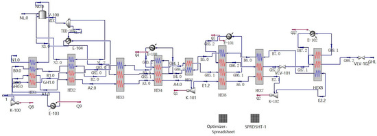
Figure 1.
HYSYS simulation (hydrogen liquefaction process).
2.8. Simulation Input Conditions and Optimized Parameter Ranges
2.8.1. Simulation Input Conditions
The parameters at each node of the hydrogen system process are shown in Table 4. The system starts from GH0.0 to GHL, with an initial material flow rate of 63 kg/h of pure hydrogen, a temperature of 300.00 K, a pressure of 2400 kPa, and a liquefaction rate of 100%.
Table 4.
Parameters of each node in the hydrogen system.
The parameters of each node in the nitrogen pre-cooling system, with a circulating nitrogen flow rate of 669 kg/h, are shown in Table 5.
Table 5.
Parameters of each node in the nitrogen pre-cooling system.
The parameters of each node in the helium refrigeration cycle are shown in Table 6. The cycle helium gas flow rate was 1505 kg/h, the initial temperature was 310 K, and the pressure was 1975 kPa.
Table 6.
Parameters of each node in the helium refrigeration cycle.
2.8.2. Optimization Setup and Parameter Ranges
The BOX (Bound Optimization by Quadratic Approximation) algorithm is a gradient-based optimization method used in Aspen HYSYS v14 to efficiently search for optimal solutions within specified variable bounds, which is particularly suitable for nonlinear engineering problems. Change A and Change B represent the maximum variable changes allowed in the initial and subsequent iterations, respectively, in the BOX optimization algorithm. Table 7 lists the setting parameters of the built-in optimizer in the HYSYS software v14.
Table 7.
Optimizer parameters.
The specific energy consumption (SEC) of the hydrogen liquefaction process depends on several parameters, including the flow rate of hydrogen and some specific parameters of the helium refrigeration cycle. The inlet temperature and the outlet pressure of the helium compressor and the flow rate of helium are critical parameters of interest because they will determine the power consumption of the helium compressor and the system efficiency of the refrigeration cycle. From a practical perspective, ensuring optimal values for these parameters can reliably improve the energy efficiency of the system and reduced operational costs. The inlet and outlet temperatures of the helium expansion machine can also have a significant impact on the SEC. Each of these temperature parameters will directly impact the power output and cooling performance of the expansion machine that is used in the helium refrigeration cycle. Given all of the aspects of system efficiency discussed above, it is paramount that these temperatures are controlled to achieve the best efficiency for the helium refrigeration cycle. That said, a low inlet temperature can enable better cooling performance of the expansion machine and an optimal outlet temperature can help maintain continuous stability in the refrigeration cycle. Table 8 shows the upper and lower limits of the parameters that could be varied.
Table 8.
Adjustable (primary) variables.
3. Energy Optimization and Analysis of Results
3.1. Optimized Energy Consumption and Load of Equipment
Table 9 presents the minimum heat transfer temperature differences for the eighth heat exchanger before and after optimization. It indicates that, following optimization, the minimum temperature differences still satisfied the constraint conditions, though some differences decreased while others increased. Detailed parameters of the heat exchanger can be found in the Appendix A.
Table 9.
Minimum temperature difference in heat exchangers after optimization. HEX1–HEX8 correspond to heat exchangers 1–8, as labeled in Figure 1.
Table 10 displays the heat transfer rates and total heat transfer rates of the heat exchanger before and after optimization. It is evident that the heat transfer rate improved following the optimization.
Table 10.
Changes in heat duty of heat exchangers after optimization.
Table 11 shows the changes in load data before and after optimization of the heater, heat exchanger, and cooler. Most loads decreased after optimization, with only a small portion increasing slightly. However, the overall load showed a downward trend.
Table 11.
Load changes.
The unit energy consumption and process performance values before and after optimization are shown in Table 12. According to Formula (2), the unit energy consumption before process optimization was 11.338 kWh/kg, while after optimization, it was 9.986 kWh/kg.
Table 12.
Changes in compressors and expanders.
3.2. Optimized Results
The parameter changes throughout the optimization process are listed in Table 13.
Table 13.
Optimized parameter values before and after optimization.
The research has indicated that factors such as hydrogen flow rate and helium cycle parameters—specifically, compressor inlet temperature, outlet pressure, and hydrogen flow—have a significant impact on energy consumption. Optimizing the total energy reduced it by 7.266% from 714.3 kW and decreased the specific energy use by 11.94% from 11.338 kWh/kg. The improved nitrogen pre-cooling and hydrogen circulation method outperforms similar techniques.
3.3. Analysis of Factors Affecting Energy Consumption
The operating parameters can directly or indirectly affect a process’s overall performance, with varying effects. To understand how the operating conditions affect liquefaction, a sensitivity analysis is needed. Next, the mass flow rate of the circulating hydrogen, the initial helium pressure, and the temperature were analyzed.
3.3.1. Effect of Hydrogen Conditions
Effect of initial hydrogen mass flow rate:
Study GH0.0: The effect of the initial hydrogen mass flow rate on the specific energy consumption while keeping all other liquefaction parameters constant was examined. Only the initial hydrogen mass flow rate was varied within the range of 60–70 kg/h, with a step size of 1 kg/h across 11 steps. The initial mass flow rate was set to 63 kg/h, and the optimized value was set as 66.34 kg/h (as shown in Table 8). Therefore, the sensitivity analysis was performed over a range of 60–70 kg/h to encompass both the baseline and optimized conditions.
As shown in Figure 2, under constant conditions, the energy consumption of the liquefaction unit decreased as the initial hydrogen flow rate increased. The Y-axis represents the specific power consumption of the liquefaction unit (in kWh/kg).
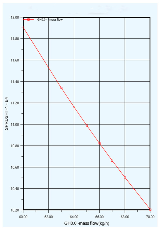
Figure 2.
Effect of initial hydrogen mass flow rate on specific energy consumption.
3.3.2. Effect of Helium Conditions
- (1)
- Effect of initial helium pressure
Study A0.0: The effect of the initial helium pressure on the specific energy consumption was investigated, with the other parameters of the fixed liquefaction process remaining constant. Only the initial helium pressure was varied, which ranged from 1950 to 2000 kPa, with a step size of 5 kPa and a total of 11 steps. The initial helium pressure was set to 1.871 MPag (≈1972 kPa), and the optimized value was set as 1.813 MPag (≈1914 kPa) (as shown in Table 8). Therefore, the sensitivity analysis was performed over the range of 1950–2000 kPa to encompass both the baseline and optimized conditions.
As shown in Figure 3, under constant conditions, the specific energy consumption of the liquefaction unit rose as the initial pressure of helium increased. The Y-axis represents the specific power consumption of the liquefaction unit (in kWh/kg), with a baseline value of 11.34 kWh/kg before optimization.
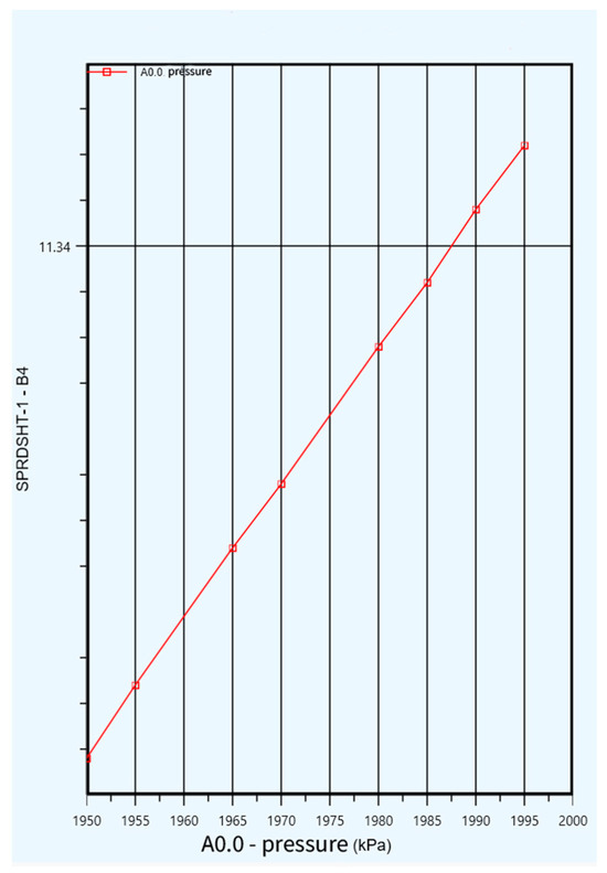
Figure 3.
Effect of initial helium pressure on energy consumption per unit.
- (2)
- Effect of initial helium temperature
Study B0.0: The effect of the initial helium temperature on the specific energy consumption was investigated, with all the other parameters of the fixed liquefaction process held constant. Only the initial helium temperature was varied, which ranged from 20 to 30 °C, with a step size of 1 °C and a total of 11 steps. The initial helium temperature was set to 24.95 °C, and the optimized value was set as 25.62 °C (as shown in Table 8). Therefore, the sensitivity analysis was performed over the range of 20–30 °C to encompass both the baseline and optimized conditions.
As shown in Figure 4, under constant conditions, the specific energy consumption of the liquefaction unit increased as the initial helium temperature increased. The Y-axis represents the specific power consumption of the liquefaction unit (in kWh/kg).
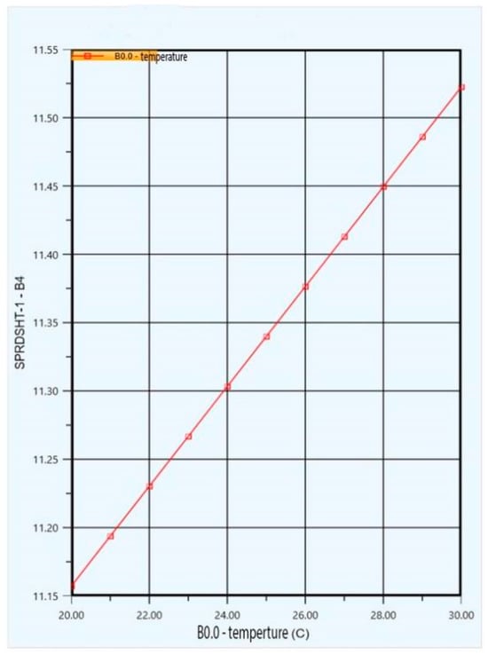
Figure 4.
Effect of initial helium temperature on specific energy consumption.
- (3)
- Effect of Pressure of Helium Entering Compressor K-100
Study Point 1: The effect of the pressure of the helium entering Compressor K-100 on the specific energy consumption was investigated. All the other parameters of the fixed liquefaction process remained constant, with only the pressure of the helium entering the compressor being varied. The pressure range was set to 1950–2000 kPa, with a step size of 5 kPa and a total of 11 steps. The initial pressure of the helium entering Compressor K-100 was set to 1.871 MPag (≈1972 kPa), and the optimized value was set as 1.703 MPag (≈1728 kPa) (as shown in Table 8). Therefore, the sensitivity analysis was performed over the range of 1950–2000 kPa to encompass the baseline and near-upper-bound conditions.
As shown in Figure 5, under consistent conditions, as the pressure of the helium entering the compressor rose, the specific energy consumption of the liquefaction unit also increased. The Y-axis represents the specific power consumption of the liquefaction unit (in kWh/kg).
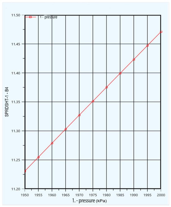
Figure 5.
Effect of pressure of helium entering Compressor K-100 on specific energy consumption.
- (4)
- Effect of temperature of helium entering the K101 expansion machine
Study A4.0: The effect of the temperature of the helium entering the K-101 expansion machine on the unit energy consumption was investigated. The other parameters of the fixed liquefaction process remained unchanged, with only the temperature of the helium entering the compressor being altered. The temperature range was set to 44.5–45.5 °k, with a step size of 0.1 K and a total of 11 steps. The initial temperature of the helium entering the K-101 expansion machine was set to 45.0 K (−228.2 °C), and the optimized value was set as the slightly lower value of 44.9 K (−228.3 °C) (as shown in Table 8). Therefore, the sensitivity analysis was performed over the range of 44.5–45.5 K to encompass both the baseline and optimized conditions.
As shown in Figure 6, when the temperature of the helium entering the expansion machine increased under constant conditions, the liquefaction system’s specific energy consumption also increased. The Y-axis represents the specific power consumption of the liquefaction unit (in kWh/kg).
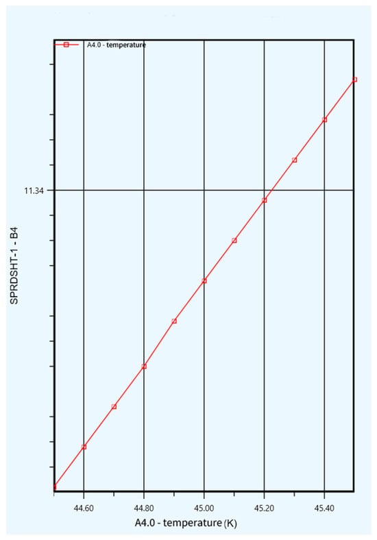
Figure 6.
Effect of temperature of helium entering the K101 expansion machine on energy consumption per unit.
- (5)
- Effect of helium temperature at inlet to expander K102
Study E2.1: The effect of the helium temperature at the inlet to expander K-102 on the specific energy consumption was investigated. All the other parameters of the fixed liquefaction process were kept constant, with only the helium temperature at the inlet to the compressor being varied. The temperature range was set to 20–30 °k, with a step size of 1 K and a total of 11 steps. The initial helium temperature at the inlet to the K-102 expander was set to 23.0 K (−250.2 °C), and the optimized value was set as the slightly lower value of 22.6 K (−250.6 °C) (as shown in Table 8). Therefore, the sensitivity analysis was performed over the range of 20–30 K to encompass both the baseline and optimized conditions.
As shown in Figure 7, when the helium inlet temperature rose under constant conditions, the liquefaction unit’s specific energy consumption increased. The Y-axis represents the specific power consumption of the liquefaction unit (in kWh/kg).
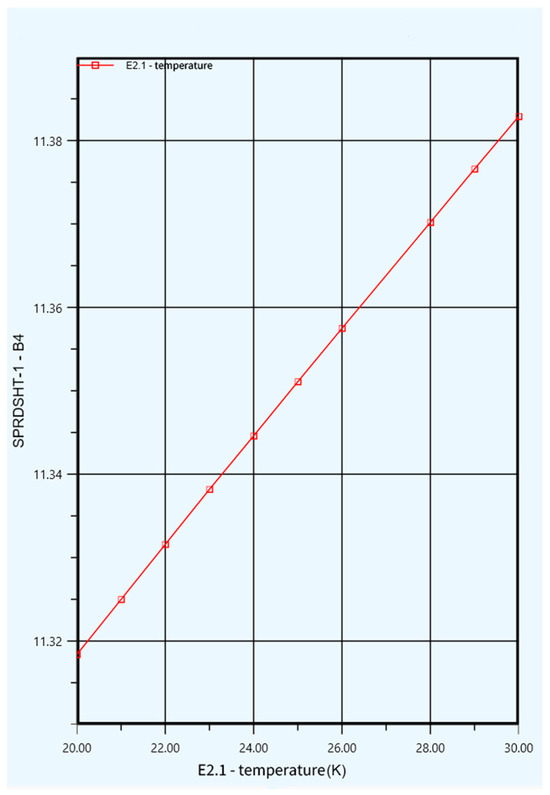
Figure 7.
Effect of helium temperature at inlet to expander K102 on specific energy consumption.
4. Conclusions
This study examined the pre-cooling Claude cycle, with the aim of reducing the energy use per product. The process operates at a pressure of 2400 kPa, temperature of 300 K, purity of 99.9999%, and a flow rate of 63 kg/h. Using Aspen HYSYS software v14, steady-state simulations were conducted to analyze the pre-cooling, refrigeration, and the transition from normal to second hydrogen liquefaction processes. Based on the energy use calculations and process analysis, a streamlined hydrogen liquefaction process flow was proposed to minimize the specific power consumption of the equipment involved.
- (1)
- After analyzing hydrogen’s properties and calculation methods, the Peng–Robinson equation was selected for the hydrogen property calculations. Considering that the equilibrium composition of normal and iso-butane hydrogen is solely a function of temperature, and that the normal hydrogen in standard hydrogen spontaneously converts to iso-butane hydrogen at lower temperatures while releasing heat, heat exchangers and heaters were added to the hydrogen liquefaction process to improve the quality of the liquid hydrogen and enhance storage safety. These devices replace the traditional normal-to-sec-hydrogen catalytic conversion reactors to eliminate the reaction heat generated during liquefaction.
- (2)
- After analyzing the various pre-cooling methods and refrigeration methods and comprehensively considering the impact of increasing the number of pre-cooling stages on energy consumption, equipment complexity, and operational maintenance costs, as well as the characteristics and feasibility of different pre-cooling agents, liquid nitrogen was ultimately selected as the pre-cooling agent. Considering equipment safety, refrigerant properties, and process design requirements, helium expansion refrigeration was selected as it can overcome multiple issues in the hydrogen liquefaction process by improving the operational efficiency, simplifying the design process, reducing the risk of equipment being affected by hydrogen embrittlement, and minimizing the impact of gas leaks on environmental and production safety. This study selected the liquid nitrogen pre-cooling system and helium refrigeration cycle for the steady-state simulations.
- (3)
- Optimization of the inlet temperature, outlet pressure, and helium mass flow rate of the helium compressor in the liquid nitrogen pre-cooling–helium expansion cycle refrigeration system was performed. Using the built-in optimizer in HYSYS, simulations were performed on different parameter combinations to determine the parameters that minimize specific energy consumption. The optimized specific energy consumption was 9.986 kWh/kg, representing a reduction of 11.94% compared to the SEC of 11.338 kWh/kg before optimization.
The reduction in specific energy consumption (SEC) after optimization was due to improved temperature matching in the multi-pass heat exchangers. It was also due to the adjustment of the intermediate pressures, which enhanced the performance of the compressor and expander.
Furthermore, the increase in mass flow rate observed in the optimized case indicates that process modifications reduce energy usage per unit product and enhance throughput, offering economic benefits. However, the simulations were conducted under steady-state and idealized conditions, which may be difficult to achieve in industrial practice. Future work should include dynamic simulations and economic analyses to validate the feasibility of these optimized parameters under realistic operating conditions.
Author Contributions
Software, J.X.; Formal analysis, J.X.; Writing—original draft, J.X.; Writing—review & editing, J.X.; Supervision, F.B. All authors have read and agreed to the published version of the manuscript.
Funding
This research received no external funding.
Data Availability Statement
All the data supporting the findings of this study are included within the article.
Conflicts of Interest
The authors declare no conflicts of interest.
Appendix A
Table A1.
Performance parameters of HEX1.
Table A1.
Performance parameters of HEX1.
| HEX1 | |||||
|---|---|---|---|---|---|
| Overall Performance | Before Optimization | After Optimization | |||
| Load (kW) | 453.9 | 456.3 | |||
| Heat Duty (kW) | 0 | 0 | |||
| Heat Loss (kW) | 0 | 0 | |||
| UA (kJ/C h) | 1.234 × 10⁵ | 1.342 × 10⁵ | |||
| Minimum Temperature Difference (°C) | 10.963 | 3.824 | |||
| LMTD (°C) | 13.24 | 12.24 | |||
| Detailed Performance | Before Optimization | After Optimization | |||
| UA Deviation Allowance (kJ/C h) | 23.94 | 284.3 | |||
| Hot-End Pinch Temperature (°C) | 35.0511 | 36.8500 | |||
| Cold-End Pinch Temperature (°C) | 24.0886 | 33.0262 | |||
| Cold-End Pinch Cold Stream Average Inlet Temperature (°C) | −195.095 | −195.095 | |||
| Hot-End Pinch Cold Stream Average Inlet Temperature (°C) | 36.850 | 36.850 | |||
| Measurement Results | |||||
| Stream Name | GH0.0–GH1.0 | B1.0–B0.0 | A0.0–A1.0 | N0.0–N1.0 | |
| Inlet Temperature (°C) | Before Optimization | 26.85 | −164.54 | 36.85 | −195.09 |
| After Optimization | 26.85 | −164.20 | 36.85 | −195.09 | |
| Outlet Temperature (°C) | Before Optimization | −160.05 | 24.95 | −150.05 | 24.09 |
| After Optimization | −160.05 | 25.62 | −150.05 | 33.03 | |
| Mass Flow Rate of Gas (Nm3/d) | Before Optimization | 16,810.50 | 202,247.73 | 202,247.73 | 12,846.86 |
| After Optimization | 177,701.64 | 202,247.73 | 202,247.73 | 12,846.86 | |
| Load (kW) | Before Optimization | −46.586 | 411.968 | −407.293 | 41.911 |
| After Optimization | −49.056 | 412.668 | −407.255 | 43.643 | |
| UA (kJ/C h) | Before Optimization | 12,833.0 | 1.12690 × 10⁵ | 1.10567 × 10⁵ | 10,710.0 |
| After Optimization | 14,582.3 | 1.22634 × 10⁵ | 1.19661 × 10⁵ | 11,608.8 | |
| Cold/Hot stream | Hot stream | Cold stream | Hot stream | Cold stream | |
Table A2.
Performance parameters of HEX2.
Table A2.
Performance parameters of HEX2.
| HEX2 | |||||
|---|---|---|---|---|---|
| Overall Performance | Before Optimization | After Optimization | |||
| Load (kW) | 125.3 | 125.7 | |||
| Heat Duty (kW) | 0 | 0 | |||
| Heat Loss (kW) | 0 | 0 | |||
| UA (kJ/C h) | 7.065 × 10⁴ | 7.375 × 10⁴ | |||
| Minimum Temperature Difference (°C) | 2.132 | 2.001 | |||
| LMTD (°C) | 6.386 | 6.138 | |||
| Detailed Performance | Before Optimization | After Optimization | |||
| UA Deviation Allowance (kJ/C h) | 15.69 | 17.98 | |||
| Hot-End Pinch Temperature (°C) | −192.9625 | −193.0936 | |||
| Cold-End Pinch Temperature (°C) | −195.0946 | −195.0946 | |||
| Cold-End Pinch Cold Stream Average Inlet Temperature (°C) | −205.435 | −205.282 | |||
| Hot-End Pinch Cold Stream Average Inlet Temperature (°C) | −150.050 | −150.050 | |||
| Measurement Results | |||||
| Stream Name | A0.0–A2.0 | B2.0–B1.0 | GH1.0–GH2.0 | NL.2–N2.0 | |
| Inlet Temperature (°C) | Before Optimization | −150.05 | −205.43 | −160.05 | −195.09 |
| After Optimization | −150.05 | −205.28 | −160.05 | −195.09 | |
| Outlet Temperature (°C) | Before Optimization | −203.15 | −164.54 | −193.15 | −195.09 |
| After Optimization | −203.15 | −164.20 | −193.15 | −195.09 | |
| Mass Flow Rate of Gas (Nm3/d) | Before Optimization | 202,247.73 | 202,247.73 | 16,810.50 | 12,674.04 |
| After Optimization | 202,247.73 | 202,247.73 | 17,701.64 | 12,674.04 | |
| Load (kW) | Before Optimization | −116.693 | 89.105 | −8.630 | 36.219 |
| After Optimization | −116.657 | 89.530 | −9.088 | 36.219 | |
| UA (kJ/C h) | Before Optimization | 67,405.8 | 51,564.5 | 3241.2 | 19,082.5 |
| After Optimization | 70,318.0 | 54,002.2 | 3437.6 | 19,753.4 | |
| Cold/Hot stream | Hot stream | Cold stream | Hot stream | Cold stream | |
Table A3.
Performance parameters of HEX3.
Table A3.
Performance parameters of HEX3.
| HEX3 | |||||
|---|---|---|---|---|---|
| Overall Performance | Before Optimization | After Optimization | |||
| Load (kW) | 42.26 | 42.59 | |||
| Heat Duty (kW) | 0 | 0 | |||
| Heat Loss (kW) | 0 | 0 | |||
| UA (kJ/C h) | 3417 × 104 | 3.488 × 10⁴ | |||
| Minimum Temperature Difference (°C) | 3.310 | 3.213 | |||
| LMTD (°C) | 4.452 | 4.395 | |||
| Detailed Performance | Before Optimization | After Optimization | |||
| UA Deviation Allowance (kJ/C h) | 27.14 | 29.98 | |||
| Hot-End Pinch Temperature (°C) | −203.1500 | −203.1500 | |||
| Cold-End Pinch Temperature (°C) | −206.4605 | −206.3630 | |||
| Cold-End Pinch Cold Stream Average Inlet Temperature (°C) | −224.760 | −224.760 | |||
| Hot-End Pinch Cold Stream Average Inlet Temperature (°C) | −195.000 | −195.000 | |||
| Measurement Results | |||||
| Stream Name | A0.0–A3.0 | B3.0–B2.0 | GH3.0–GH3.1 | ||
| Inlet Temperature (°C) | Before Optimization | −203.15 | −224.76 | −195.00 | |
| After Optimization | −203.15 | −224.76 | −195.00 | ||
| Outlet Temperature (°C) | Before Optimization | −219.15 | −205.43 | −218.15 | |
| After Optimization | −219.15 | −205.28 | −218.15 | ||
| Mass Flow Rate of Gas (Nm3/d) | Before Optimization | 202,247.73 | 202,247.73 | 16,810.50 | |
| After Optimization | 202,247.73 | 202,247.73 | 17,701.64 | ||
| Load (kW) | Before Optimization | −35.594 | 42.256 | −6.662 | |
| After Optimization | −35.572 | 42.589 | −7.015 | ||
| UA (kJ/C h) | Before Optimization | 29,414.7 | 34,172.3 | 4757.6 | |
| After Optimization | 29,798.0 | 34,885.1 | 5087.1 | ||
| Cold/Hot stream | Hot stream | Cold stream | Hot stream | ||
Table A4.
Performance parameters of HEX4.
Table A4.
Performance parameters of HEX4.
| HEX4 | |||||
|---|---|---|---|---|---|
| Overall Performance | Before Optimization | After Optimization | |||
| Load (kW) | 24.32 | 24.32 | |||
| Heat Duty (kW) | 0 | 0 | |||
| Heat Loss (kW) | 0 | 0 | |||
| UA (kJ/C h) | 1.254 × 10⁴ | 1258 × 104 | |||
| Minimum Temperature Difference (°C) | 5.903 | 5.919 | |||
| LMTD (°C) | 6.984 | 6.957 | |||
| Detailed Performance | Before Optimization | After Optimization | |||
| UA Deviation Allowance (kJ/C h) | 1.660 | 4.791 | |||
| Hot-End Pinch Temperature (°C) | −219.1500 | −219.1500 | |||
| Cold-End Pinch Temperature (°C) | −225.0531 | −225.0685 | |||
| Cold-End Pinch Cold Stream Average Inlet Temperature (°C) | −235.830 | −235.830 | |||
| Hot-End Pinch Cold Stream Average Inlet Temperature (°C) | −218.150 | −218.150 | |||
| Measurement Results | |||||
| Stream Name | A3.0–A4.0 | B4.0–B3.0 | GH3.1–GH3.0 | GH3.1–GH4.1 | |
| Inlet Temperature (°C) | Before Optimization | −219.15 | −235.83 | −218.15 | −218.15 |
| After Optimization | −219.15 | −235.83 | −218.15 | −218.15 | |
| Outlet Temperature (°C) | Before Optimization | −228.15 | −224.76 | −225.17 | −223.15 |
| After Optimization | −228.33 | −224.76 | −223.62 | −223.15 | |
| Mass Flow Rate of Gas (Nm3/d) | Before Optimization | 202,247.73 | 202,247.73 | 16,810.50 | 16,810.50 |
| After Optimization | 202,247.73 | 202,247.73 | 17,701.64 | 17,701.64 | |
| Load (kW) | Before Optimization | −20.247 | 24.319 | −2.404 | −1.668 |
| After Optimization | −20.629 | 24.319 | −1.933 | −1.757 | |
| UA (kJ/C h) | Before Optimization | 10,400.9 | 12,536.2 | 1246.2 | 889.0 |
| After Optimization | 10,688.5 | 12,583.8 | 990.9 | 904.3 | |
| Cold/Hot stream | Hot stream | Cold stream | Hot stream | Hot stream | |
Table A5.
Performance parameters of HEX5.
Table A5.
Performance parameters of HEX5.
| HEX5 | |||
|---|---|---|---|
| Overall Performance | Before Optimization | After Optimization | |
| Load (kW) | 5.205 | 5.205 | |
| Heat Duty (kW) | 0 | 0 | |
| Heat Loss (kW) | 0 | 0 | |
| UA (kJ/C h) | 2708 | 2582 | |
| Minimum Temperature Difference (°C) | 4.056 | 4.438 | |
| LMTD (°C) | 6.920 | 7.256 | |
| Detailed Performance | Before Optimization | After Optimization | |
| UA Deviation Allowance (kJ/C h) | 1.910 | 1.678 | |
| Hot-End Pinch Temperature (°C) | −234.1345 | −233.7519 | |
| Cold-End Pinch Temperature (°C) | −238.1900 | −238.1900 | |
| Cold-End Pinch Cold Stream Average Inlet Temperature (°C) | −238.190 | −238.190 | |
| Hot-End Pinch Cold Stream Average Inlet Temperature (°C) | −223.150 | −223.150 | |
| Measurement Results | |||
| Stream Name | B5.0 | GH4.2–GH5.1 | |
| Inlet Temperature (°C) | Before Optimization | −238.19 | −223.15 |
| After Optimization | −238.19 | −223.15 | |
| Outlet Temperature (°C) | Before Optimization | −235.83 | −234.13 |
| After Optimization | −235.83 | −233.75 | |
| Mass Flow Rate of Gas (Nm3/d) | Before Optimization | 202,247.73 | 16,810.50 |
| After Optimization | 202,247.73 | 17,701.64 | |
| Load (kW) | Before Optimization | 5.205 | −5.205 |
| After Optimization | 5.204 | −5.204 | |
| UA (kJ/C h) | Before Optimization | 2707.6 | 2707.6 |
| After Optimization | 2582.7 | 2582.7 | |
| Cold/Hot stream | Cold stream | Hot stream | |
Table A6.
Performance parameters of HEX6.
Table A6.
Performance parameters of HEX6.
| HEX6 | |||||
|---|---|---|---|---|---|
| Overall Performance | Before Optimization | After Optimization | |||
| Load (kW) | 21.20 | 21.20 | |||
| Heat Duty (kW) | 0 | 0 | |||
| Heat Loss (kW) | 0 | 0 | |||
| UA (kJ/C h) | 2.910 × 10⁴ | 2.881 × 10⁴ | |||
| Minimum Temperature Difference (°C) | 2.133 | 2.089 | |||
| LMTD (°C) | 2.623 | 2.648 | |||
| Detailed Performance | Before Optimization | After Optimization | |||
| UA Deviation Allowance (kJ/C h) | 52.95 | 51.11 | |||
| Hot-End Pinch Temperature (°C) | −238.5384 | −238.3590 | |||
| Cold-End Pinch Temperature (°C) | −240.6710 | −240.4475 | |||
| Cold-End Pinch Cold Stream Average Inlet Temperature (°C) | −247.740 | −247.740 | |||
| Hot-End Pinch Cold Stream Average Inlet Temperature (°C) | −234.134 | −233.752 | |||
| Measurement Results | |||||
| Stream Name | E1.2–A6.0 | B6.0–B5.0 | GH5.1–GH6.1 | GH5.2–GH6.2 | |
| Inlet Temperature (°C) | Before Optimization | −238.54 | −247.74 | −234.13 | −234.15 |
| After Optimization | −238.36 | −247.74 | −233.75 | −234.15 | |
| Outlet Temperature (°C) | Before Optimization | −245.15 | −238.19 | −240.15 | −238.63 |
| After Optimization | −245.15 | −238.19 | −240.15 | −238.88 | |
| Mass Flow Rate of Gas (Nm3/d) | Before Optimization | 202,247.73 | 202,247.73 | 16,810.50 | 16,810.50 |
| After Optimization | 202,247.73 | 202,247.73 | 17,701.64 | 17,701.64 | |
| Load (kW) | Before Optimization | −14.914 | 21.198 | −3.502 | −2.782 |
| After Optimization | −15.316 | 21.198 | −3.965 | −1.917 | |
| UA (kJ/C h) | Before Optimization | 22,038.3 | 29,098.7 | 4075.9 | 2984.5 |
| After Optimization | 22,607.6 | 28,813.6 | 4212.0 | 1994.0 | |
| Cold/Hot stream | Hot stream | Cold stream | Hot stream | Hot stream | |
Table A7.
Performance Parameters of HEX7.
Table A7.
Performance Parameters of HEX7.
| HEX7 | |||||
|---|---|---|---|---|---|
| Overall Performance | Before Optimization | After Optimization | |||
| Load (kW) | 12.64 | 12.64 | |||
| Heat Duty (kW) | 0 | 0 | |||
| Heat Loss (kW) | 0 | 0 | |||
| UA (kJ/C h) | 1.363 × 10⁴ | 1.721 × 10⁴ | |||
| Minimum Temperature Difference (°C) | 3.109 | 2.592 | |||
| LMTD (°C) | 3.339 | 2.645 | |||
| Detailed Performance | Before Optimization | After Optimization | |||
| UA Deviation Allowance (kJ/C h) | 6.238 × 10⁻³ | 0.1984 | |||
| Hot-End Pinch Temperature (°C) | −245.1500 | −245.1500 | |||
| Cold-End Pinch Temperature (°C) | −248.2586 | −247.7420 | |||
| Cold-End Pinch Cold Stream Average Inlet Temperature (°C) | −253.350 | −253.350 | |||
| Hot-End Pinch Cold Stream Average Inlet Temperature (°C) | −238.626 | −236.877 | |||
| Measurement Results | |||||
| Stream Name | A6.0–E2.1 | B7.0–B6.0 | GH6.2–GH7.0 | ||
| Inlet Temperature (°C) | Before Optimization | −245.15 | −253.35 | −238.63 | |
| After Optimization | −245.15 | −253.35 | −238.88 | ||
| Outlet Temperature (°C) | Before Optimization | −250.15 | −247.74 | −241.23 | |
| After Optimization | −250.65 | −247.74 | −236.88 | ||
| Mass Flow Rate of Gas (Nm3/d) | Before Optimization | 202,247.73 | 202,247.73 | 16,810.50 | |
| After Optimization | 202,247.73 | 202,247.73 | 17,701.64 | ||
| Load (kW) | Before Optimization | −11.482 | 12.642 | −1.160 | |
| After Optimization | −12.637 | 12.642 | −0.005 | ||
| UA (kJ/C h) | Before Optimization | 13112.7 | 13630.0 | 517.4 | |
| After Optimization | 17204.0 | 17205.5 | 1.5 | ||
| Cold/Hot stream | Hot stream | Cold stream | Hot stream | ||
Table A8.
Performance parameters of HEX8.
Table A8.
Performance parameters of HEX8.
| HEX8 | |||||
|---|---|---|---|---|---|
| Overall Performance | Before Optimization | After Optimization | |||
| Load (kW) | 2.715 | 5.087 | |||
| Heat Duty (kW) | 0 | 0 | |||
| Heat Loss (kW) | 0 | 0 | |||
| UA (kJ/C h) | 1383 | 2640 | |||
| Minimum Temperature Difference (°C) | 4.269 | 3.787 | |||
| LMTD (°C) | 7.064 | 6.939 | |||
| Detailed Performance | Before Optimization | After Optimization | |||
| UA Deviation Allowance (kJ/C h) | 0.6906 | 1.275 | |||
| Hot-End Pinch Temperature (°C) | −250.1500 | −239.6518 | |||
| Cold-End Pinch Temperature (°C) | −254.4189 | −243.4386 | |||
| Cold-End Pinch Cold Stream Average Inlet Temperature (°C) | −254.419 | −254.834 | |||
| Hot-End Pinch Cold Stream Average Inlet Temperature (°C) | −242.194 | −239.652 | |||
| Measurement Results | |||||
| Stream Name | GH7.1–GH8.1 | E2.2–B7.0 | GH7.2–GH8.2 | ||
| Inlet Temperature (°C) | Before Optimization | −242.19 | −254.42 | −248.15 | |
| After Optimization | −239.65 | −254.83 | −248.15 | ||
| Outlet Temperature (°C) | Before Optimization | −250.15 | −253.35 | −247.19 | |
| After Optimization | −250.15 | −253.35 | −243.44 | ||
| Mass Flow Rate of Gas (Nm3/d) | Before Optimization | 16,810.50 | 202,247.73 | 16,810.50 | |
| After Optimization | 17,701.64 | 202,247.73 | 17,701.64 | ||
| Load (kW) | Before Optimization | −2.715 | 2.439 | 0.276 | |
| After Optimization | −5.087 | 3.390 | 1.697 | ||
| UA (kJ/C h) | Before Optimization | 1383.4 | 1192.2 | 191.2 | |
| After Optimization | 2639.5 | 1446.4 | 1193.1 | ||
| Cold/Hot stream | Hot stream | Cold stream | Cold stream | ||
References
- Al Ghafri, S.Z.; Munro, S.; Cardella, U.; Funke, T.; Notardonato, W.; Trusler, J.P.M.; Leachman, J.; Span, R.; Kamiya, S.; Pearce, G.; et al. Hydrogen Liquefaction: A Review of the Fundamental Physics, Engineering Practice and Future Opportunities. Energy Environ. Sci. 2022, 15, 2690–2731. [Google Scholar] [CrossRef]
- Chirosca, A.-M.; Rusu, E.; Minzu, V. Green hydrogen—Production and storage methods: Current status and future directions. Energies 2024, 17, 5820. [Google Scholar] [CrossRef]
- Aziz, M. Liquid hydrogen: A review on liquefaction, storage, transportation, and safety. Energies 2021, 14, 5917. [Google Scholar] [CrossRef]
- Zhang, T.; Uratani, J.; Huang, Y.; Xu, L.; Griffiths, S.; Ding, Y. Hydrogen liquefaction and storage: Recent progress and perspectives. Renew. Sustain. Energy Rev. 2023, 176, 113204. [Google Scholar] [CrossRef]
- Baker, C.H.; Sage, B.H. Hydrogen liquefaction by the Claude process. Ind. Eng. Chem. 1954, 46, 1940–1945. [Google Scholar] [CrossRef]
- Quack, H. Conceptual design of a high efficiency large capacity hydrogen liquefier. AIP Conf. Proc. 2002, 613, 255–263. [Google Scholar] [CrossRef]
- Kuz’menko, I.F.; Morkovkin, I.M.; Gurov, E.I. Concept of Building Medium-Capacity Hydrogen Liquefiers with Helium Refrigeration Cycle. Chem. Pet. Eng. 2004, 40, 94–98. [Google Scholar] [CrossRef]
- Berstad, D.O.; Stang, J.H.; Nekså, P. Large-scale hydrogen liquefier utilising mixed-refrigerant pre-cooling. Int. J. Hydrogen Energy 2010, 35, 4519–4525. [Google Scholar] [CrossRef]
- Valenti, G.; Macchi, E. Proposal of an innovative, high-efficiency, large-scale hydrogen liquefier. Int. J. Hydrogen Energy 2008, 33, 3116–3121. [Google Scholar] [CrossRef]
- Asadnia, M.; Mehrpooya, M. A novel hydrogen liquefaction process configuration with combined mixed refrigerant systems. Int. J. Hydrogen Energy 2017, 42, 15564–15585. [Google Scholar] [CrossRef]
- Sadaghiani, M.S.; Mehrpooya, M. Introducing and energy analysis of a novel cryogenic hydrogen liquefaction process configuration. Int. J. Hydrogen Energy 2017, 42, 6033–6050. [Google Scholar] [CrossRef]
- Yin, L.; Ju, Y. Process optimization and analysis of a novel hydrogen liquefaction cycle. Int. J. Refrig. 2020, 110, 219–230. [Google Scholar] [CrossRef]
- Riaz, A.; Qyyum, M.A.; Min, S.; Lee, S.; Lee, M. Performance improvement potential of harnessing LNG regasification for hydrogen liquefaction process: Energy and exergy perspectives. Appl. Energy 2021, 301, 117471. [Google Scholar] [CrossRef]
- Naquash, A.; Qyyum, M.A.; Min, S.; Lee, S.; Lee, M. Carbon–dioxide–precooled hydrogen liquefaction process: An innovative approach for performance enhancement—Energy, exergy, and economic perspectives. Energy Convers. Manag. 2022, 251, 114947. [Google Scholar] [CrossRef]
- Wang, G.C.; Xu, Z.L.; Duo, Z.L.; Zhu, J.L.; Li, Y.X. Optimization of mixed-refrigerant hydrogen liquefaction process. J. Northeast. Electr. Power Univ. 2021, 41, 61–70. [Google Scholar] [CrossRef]
- Wang, C.; Sun, H.; Geng, J.L.; Rong, G.; Ren, R. Optimization of dual mixed-refrigerant hydrogen liquefaction process based on PSO algorithm. Cryog. Supercond. 2021, 49, 96–102. [Google Scholar] [CrossRef]
- Bi, Y.; Yin, L.; He, T.; Ju, Y. Optimization and analysis of a novel hydrogen liquefaction process for circulating hydrogen refrigeration. Int. J. Hydrogen Energy 2022, 47, 348–364. [Google Scholar] [CrossRef]
- Naquash, A.; Qyyum, M.A.; Islam, M.; Sial, N.R.; Min, S.; Lee, S.; Lee, M. Performance enhancement of hydrogen liquefaction process via absorption refrigeration and organic Rankine cycle-assisted liquid air energy system. Energy Convers. Manag. 2022, 254, 115200. [Google Scholar] [CrossRef]
- Zhang, S.; Liu, G. Design and performance analysis of a hydrogen liquefaction process. Clean Technol. Environ. Policy 2022, 24, 51–65. [Google Scholar] [CrossRef]
- Wang, H.; Yang, J.; Dong, X.; Gong, M. Current status of hydrogen liquefaction and cryogenic high-pressure hydrogen storage technologies. Clean Coal Technol. 2023, 29, 102–113. [Google Scholar] [CrossRef]
- Mahboobtosi, H.; Ganji, D.D.; Gorji, M.; Hosseinzadeh, K. Investigation and thermodynamic analysis of hydrogen liquefaction cycles: Energy and exergy study. Heliyon 2024, 10, e37570. [Google Scholar] [CrossRef]
- Air Products. Air Products’ New World-Scale Liquid Hydrogen Plant is Onstream at Its La Porte, Texas Facility. Available online: https://www.airproducts.com/company/news-center/2021/10/1007-air-products-new-liquid-hydrogen-plant-onstream-at-laporte-texas-facility (accessed on 13 August 2025).
- Reuters. Air Products to Launch 30 Tonnes per Day Liquid Hydrogen Plants in China in 2022. Reuters. 2020. Available online: https://www.reuters.com/article/business/energy/air-products-to-launch-30-tonnes-per-day-liquid-hydrogen-plants-in-china-in-2022-idUSKBN27Q12T (accessed on 13 August 2025).
- Plug Power. Plug Power Starts Production of Liquid Green Hydrogen at Its Georgia Plant. Available online: https://www.ir.plugpower.com/press-releases/news-details/2024/Plug-Power-Starts-Production-of-Liquid-Green-Hydrogen-at-its-Georgia-Plant/default.aspx (accessed on 13 August 2025).
- Doosan Enerbility. Doosan Enerbility Attends Ceremony to Celebrate Construction Completion of “Changwon Hydrogen Liquefaction Plant”. Doosan, 31 January 2024. Available online: https://www.doosan.com/en/media-center/press-release_view?id=20172562 (accessed on 13 August 2025).
- Cardella, U.; Decker, L.; Klein, H. Roadmap to economically viable hydrogen liquefaction. Int. J. Hydrogen Energy 2017, 42, 13329–13338. [Google Scholar] [CrossRef]
- Leachman, J.W.; Jacobsen, R.T.; Lemmon, E.W.; Penoncello, S.G. Fundamental equations of state for parahydrogen, normal hydrogen, and orthohydrogen. J. Phys. Chem. Ref. Data 2009, 38, 721–748. [Google Scholar] [CrossRef]
Disclaimer/Publisher’s Note: The statements, opinions and data contained in all publications are solely those of the individual author(s) and contributor(s) and not of MDPI and/or the editor(s). MDPI and/or the editor(s) disclaim responsibility for any injury to people or property resulting from any ideas, methods, instructions or products referred to in the content. |
© 2025 by the authors. Licensee MDPI, Basel, Switzerland. This article is an open access article distributed under the terms and conditions of the Creative Commons Attribution (CC BY) license (https://creativecommons.org/licenses/by/4.0/).