Abstract
In this paper, we present a distributed low-carbon demand response method in distribution networks incorporating day-ahead and intraday flexibilities on the demand side. This two-stage demand dispatch scheme, including day-ahead schedule and intraday adjustment, is proposed to facilitate the coordination between power demand and local photovoltaic (PV) generation. We employ the alternating direction method of multipliers (ADMM) to solve the dispatch problem in a distributed manner. Demand response in a 141-bus test system serves as our case study, demonstrating the effectiveness of our approach in shifting power loads to periods of high PV generation. Our results indicate remarkable reductions in the total carbon emission by utilizing more distributed PV generation.
1. Introduction
In conventional power systems, the electricity supply is mainly provided by fossil fuel power plants. The traditional fossil energy sources used by these power plants emit large amounts of carbon dioxide and cause environmental pollution during production and conversion [1]. However, in recent years, renewable energy power generation has been developing rapidly, and new power systems have emerged, low-carbonization will be one of the main features of future new power systems. Although renewable energy power generation does not cause carbon emissions, it has intermittency and uncertainty [2,3,4], its power output depends on fluctuating meteorological conditions such as wind speed and solar radiation, which brings new challenges to the safe and economic operation of power systems. At the same time, there is a temporal and spatial mismatch between renewable energy power generation and actual electricity demand, and extreme weather events and strategic power producers also pose challenges to the power market [5,6]. Under this changing trend, new power systems have gradually become a research focus, and demand response has also become an important strategy for shifting electricity demand and promoting the use of low-carbon renewable energy power generation.
In the new power system, the electricity consumption is one of the sources of carbon emissions. Hence, relevant scholars are dedicated to researching ways and methods to reduce the carbon emissions of the system from the power supply side. Among them, demand response is a mechanism that adjusts electricity demand to adapt to the instability of renewable energy generation, thereby managing the carbon emissions produced by the power system. References [7,8] introduced the carbon trading mechanism model into the integrated energy system, proposed a stepwise demand response mechanism model, and constructed a low-carbon economic optimization model for the integrated energy system, effectively reducing the carbon operation cost of industrial parks and achieving the low-carbon and efficient utilization of demand-side flexibility resources. However, the abovementioned literature is based on carbon reduction technologies such as carbon capture power plants and multi-energy complementary power systems, using demand response as a dispatchable resource to cooperate with source-side carbon reduction for the low-carbon economic dispatch of the entire power system, rather than the traditional demand response low-carbon dispatch research based on the carbon potential of each node in the power system. Therefore, the scholars in article [9] have introduced the theory of carbon emission flow and conducted research on carbon emission behavior from the demand side. The authors of [10,11] introduced the method for calculating carbon emission flow and achieved the transformation from power flow to “carbon emission flow” through specific modeling, analyzing the characteristics of carbon emission flow distribution with power flow, and achieving the best management of energy consumption and carbon emissions on the demand side. However, existing studies have separately introduced market mechanisms or power flow analysis to analyze carbon emissions, and there has been insufficient research on carbon emission constraint optimization at the distribution network level. Therefore, further research is needed on how to combine demand response loads with flexible regulation capabilities with multi-timescale optimization dispatch models for distribution networks that include carbon emission targets, so as to cooperatively improve system economics and low-carbon performance.
At the same time, due to the large number of loads involved in demand response, the existing centralized optimization scheduling method cannot meet the carbon emission models required by different operating entities, and there are also obvious shortcomings in the scale and computational efficiency of problem solving [12]. On this basis, distributed optimization algorithms such as alternating direction method of multipliers (ADMM) [13] and analytical target cascading (ATC) [14] have been widely used to solve multi-agent low-carbon model-solving problems. The alternating direction multiplier method has been widely used in distributed solutions due to its advantages such as high convergence accuracy, short solution time, global convergence, and easy implementation [15]. Reference [16] proposed a fully distributed economic dispatch algorithm based on ADMM to optimize the power generation, demand, and pricing decisions of operators. The authors of [17] used cluster-based distributed ADMM to develop a demand response strategy for a campus load allocation problem. The article [18] developed a distributed optimization algorithm based on ADMM for greenhouse networks, which effectively realized load transfer. The authors of [19] considered the uncertainty of day-ahead and intraday demand response and load, proposed an economic optimization model based on Stackelberg game theory, and successfully reduced operating costs. The authors of [20] integrated IoT devices, thermostatic control loads, and electric vehicles in smart residential buildings and used the ADMM algorithm to achieve economic and global optimization. The authors of [21] proposed a cooperative game pricing method based on the ADMM algorithm, allowing customers to participate in demand response to alleviate transmission congestion during peak hours.
Although the research mentioned above used the distributed algorithm for optimization, most of them focused on economic efficiency as the optimization objective, with little consideration given to environmental factors. Carbon emissions were not incorporated into the objective function, and there is limited research on constraint optimization scheduling that accounts for carbon emissions in demand-side response. Although the authors of [22] proposed a storage coordination control strategy with operational costs and carbon emissions as optimization objectives, their approach did not consider load flexibility. The authors of [23] designed a day-ahead and intraday optimization model considering the uncertainty of source-load, successfully minimizing the system’s energy purchase, operational, and carbon emission costs, but did not address the optimization algorithm. Therefore, these methods all have obvious limitations when it comes to solving demand response problems involving carbon emissions.
In summary, this paper focuses on the source-load mismatch problem in distribution networks. Based on predicted source-load data and distributed solution algorithms, it quantifies the demand response capacity of distribution grids and reduces overall carbon emissions through a two-stage demand response method that combines day-ahead and intraday scheduling. The main research contributions are as follows:
- Considering the combination of day-ahead scheduling and intraday adjustment of demand response, we proposed a two-stage demand response strategy. This strategy can utilize the flexible load with faster response ability to handle deviations of actual local photovoltaic (PV) generation from the day-ahead forecast, thereby promoting the integration and accommodation of photovoltaic power generation.
- We proposed a distributed demand response mechanism based on ADMM. Users iteratively exchange their schedules with operators to obtain optimal demand schedules. The warm-start intraday adjustment strategy uses day-ahead schedules to accelerate convergence and enables efficient re-scheduling when the PV generation fluctuates.
Finally, the IEEE-141 test system is used as a case to validate the effectiveness of the proposed strategy and mechanism.
The remainder of this paper is organized as follows. The mathematical model of low-carbon demand response is introduced in Section 2. The distributed solution method for day-ahead schedule and intraday adjustment is presented in Section 3. A case study and results are presented in Section 4. Conclusions are drawn in Section 5.
2. Mathematical Model of Low-Carbon Demand Response
2.1. Objective Functions
In our low-carbon demand response model, we consider two kinds of objectives to optimize: the carbon emission and the economic compensation of demand response.
2.1.1. Carbon Emission
The total carbon emission in one period t is divided into two parts: (1) the emission caused by local generators and (2) the carbon emission of the transmission network. Considering the inevitable power exchange between a distribution network and transmission network, we regard the transmission network as a single power source.
Here, denotes the emission function of local generator with respect to its power output , which can be expressed as a linear function. The emission factor depends on the type of generator. For distributed photovoltaic generation, we can regard them as zero-carbon power sources with emission factor .
denotes the average carbon emission factor of the power of transmission network. It can be regarded as the weighted average of all kinds of power sources such as thermal generation, hydraulic generation, and wind power generation.
2.1.2. Compensation of Demand Response
The power demand of flexible load is adjustable and the economic compensation for demand response is dependent on the deviation between the actual load and its baseline power load . In this analysis, we adopt a piecewise compensation cost when the depth of demand response lies in different intervals.
For example, the compensation price for response around baseline is listed in Table 1:

Table 1.
Piecewise compensation price for demand response.
The compensation for demand response in this case can be written as:
Because the compensation price usually grows higher as the depth of demand response increases (), the compensation is a convex function with respect to the actual load , which allows us to rewrite the piecewise function as a series of equivalent linear constraints.
2.2. Constraints
2.2.1. Generator and DG Output Constraints
Constraints (9) and (10) restrict the active power and reactive power of local generators such as distributed photovoltaic generation. The maximal power output of photovoltaic generation is restricted by the solar radiation and its time variation.
2.2.2. Power Flow Constraints
We use the linear branch flow model to describe the power flow constraints in a radial distribution network:
where , and denote active and reactive power flow of a branch, and denotes the square of bus voltage magnitude. Constraints (11) and (12) are equivalent to the power balance equation of bus , and (13) describes the voltage fall of branch .
2.2.3. Branch Capacity Constraints
This is a second-order cone constraint to limit the power flow below the capacity of the branch.
2.2.4. Voltage Constraints
In Equation (16), the voltage at the bus connected to the transmission network, numbered bus-0, is known as the reference voltage.
2.2.5. Demand Response Constraints
The adjustment of flexible power load in demand response is restricted by its internal physical constraints. Here, we consider the upper and lower bounds of power and energy consumed by adjustable load via the virtual battery model.
2.3. Day-Ahead and Intraday Demand Response Model
The flexible load in practice can be divided into two categories according to their response ability: load with day-ahead flexibility and load with intraday flexibility. Their differences are summarized as follows:
- The load with day-ahead flexibility can only participate in the invitation of demand response for the next day and prepare the production schedule to alter their load in advance. As a result, they cannot respond to short-term intraday demand response.
- Alternatively, the load with intraday flexibility can adjust its power demand with a shorter response delay such as several hours, so it can take part in the intraday demand response to schedule its load during the rest of the day. The fast response ability of a load with intraday flexibility also means that its compensation rate is higher than a load with day-ahead flexibility.
Considering the different characteristics of flexible loads, we propose a two-stage demand response scheme that includes a day-ahead schedule and intraday adjustment.
In the day-ahead stage, the demand response model aims to optimize the total carbon emission and compensation for a load with day-ahead flexibility during the whole day. The objective is written as follows:
The constraints in the day-ahead model include (1)–(19), where the subscript of time t ranges from time 1 to T. The maximal power output of photovoltaic generation in constraint (9) is obtained via the day-ahead forecast. Only the load with day-ahead flexibility is adjustable, as restricted by constraints (17)–(19), while the load with intraday flexibility strictly follows its baseline power demand curve.
During the next day, the actual power demand of the load with day-ahead flexibility might deviate from its previously determined trajectory. Furthermore, the inaccurate day-ahead forecast will underestimate or overestimate the actual photovoltaic generation. As the result, the day-ahead demand response may be insufficient to maintain the low-carbon and secure operation of the distribution network and requires intraday adjustment to explore for more flexibility on the load side.
In the intraday stage, the demand response model aims to optimize the total carbon emission and compensation for the load with intraday flexibility during the rest of the day (after the m-th time point).
The constraints in intraday model include (1)–(16), where the subscript of time t ranges from time m to T. The maximal power output of photovoltaic generation in constraint (9) is updated by intraday forecast with the latest solar radiation data.
For the load with day-ahead flexibility, its power demand is assumed to follow the actual response trajectory.
For the load with intraday flexibility, its power demand is only adjustable after the response delay , as constrained by (23)–(26).
Remark 1.
Multiple established methods exist for predicting baseline loads, including statistical approaches (e.g., averaging method, linear regression [24]); machine learning algorithms (e.g., support vector regression (SVR) [25]); and deep learning frameworks (e.g., LSTM with demand response deviation correction [26], Deep-Autoformer [27]). Recent advances even integrate generative pre-trained transformers (GPT) with weighted averaging for short-term load forecasting [28].
Remark 2.
This study adopts the averaging method from [24] to determine baseline loads. While we acknowledge that this approach may exhibit lower accuracy compared to advanced machine/deep learning models ([25,26,27,28]), its computational efficiency and widespread adoption in engineering practice align with our primary objective: validating the proposed demand response strategy, rather than optimizing prediction methods.
3. The Distributed Solution Algorithm of Day-Ahead and Intraday Demand Response
The low-carbon demand response model proposed in the previous section is a second-order cone programming problem. Although it can be solved by collecting information from all the flexible loads, the centralized solution process is faced with several challenging aspects:
- The mechanism of demand response in practice is naturally distributed. After the operator announces the invitation of demand response to all potential participants, only a fraction of flexible loads will participate and send back the altered load schedule as a response. Thus, a distributed algorithm is more appropriate for the volunteering participation nature of demand response than the centralized optimize-then-dispatch approach.
- It is difficult to acquire and maintain accurate parameters of all flexible loads on the demand side, especially when it contains sensitive private information. The centralized demand response model cannot be solved with partial observability of the demand side.
- The number of flexible loads is huge, so the computational efficiency of the centralized model will degrade when the size of variables and constraints increases.
Therefore, we propose in this paper a distributed demand response mechanism based on the alternating direction multiplier method (ADMM) to circumvent the drawbacks of a centralized solution procedure.
Figure 1 shows the flowchart of a distributed solution algorithm of day-ahead and intraday demand response. In the day-ahead scheduling stage, an optimal scheduling plan with a time scale of 24 h is developed through load forecast data and renewable energy forecast data. In the intraday scheduling stage, a rolling optimal scheduling plan with a time scale of 60 min is developed through actual load and renewable energy output, which are coupled by the unit output baseline load. At the same time, the global optimal solution of scheduling plan is obtained by the ADMM algorithm.
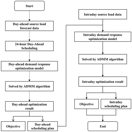
Figure 1.
Multi-timescale distributed solution algorithm and demand response optimization scheduling flowchart.
3.1. Introduction to the ADMM Algorithm
We firstly give a brief introduction to the ADMM algorithm, which can be used to solve the following two-part form of a problem that includes decision variables and .
After introducing the augmented Lagrangian function and dual multiplier , the optimal solution can be obtained iteratively by updating the primal variables and dual multiplier .
3.2. Reformulation of the Demand Response Model as Consensus Optimization
To apply ADMM to the demand response model, we introduce two artificial copies of power-load variables :
- (1)
- Grid-side power load: ;
- (2)
- Load-side power load: ;
The decision variables are also separated into two parts:
- (1)
- Grid-side variables: ;
- (2)
- Load-side variables: ;
Using the day-ahead demand response as an example, we can rewrite the low-carbon demand response model as a consensus optimization problem. The objective function remains unchanged, and the constraints are divided into three categories:
3.2.1. Public Constraints on the Grid Side
The public constraints on the grid side include constraints (1)–(16), where the power load in piecewise response compensation constraints (5)–(8) and power flow constraints (11) and (12) are substituted by their grid-side variants . These constraints only contain the information known by the grid operators and the decision variables on the grid side.
3.2.2. Local Constraints on the Load Side
The local constraints include the demand response constraints of a single load, where the power-load variables are substituted by their load-side variants . These constraints determine the adjustable flexibility of each load, which only contain the information known by owner of the load and the decision variables on the load side.
3.2.3. Consensus Constraints
To obtain the final solution of the optimal demand response, the power load in public constraints on the grid side and local constraints on the load side should be equal to each other. This is equivalent to the coupling constraint (28) in ADMM.
3.3. Day-Ahead Distributed Solution Algorithm
Based on the consensus optimization form, we can use the ADMM algorithm to design a distributed demand response mechanism to determine the day-ahead schedule.
Step 1 (Initialization): Initialize the power load for all loads with day-ahead flexibility on both sides with their forecast baseline and the dual multipliers . Because not all loads with day-ahead flexibility participate in the demand response, they are divided into two sets: (1) loads that participate in demand response ; (2) loads that do not participate in demand response . In the beginning, we assume that no loads will participate, and the sets will be updated progressively.
Step 2 (Global coordination): Solve the coordinated day-ahead demand response model with augmented terms and public constraints on the grid side.
Except for constraints (1)–(16), the loads that do not participate in demand response are assumed to follow their baseline load, which introduces extra constraints.
After solving the coordinated day-ahead demand response model, the coordinator of demand response sends privately the result for the grid-side power load and corresponding dual multipliers for each flexible load.
Step 3 (Local response): The power load on the load side are updated as in (31) with the following objective, where the values of and are obtained from step 2.
The constraints include (33)–(35). We notice that the objective function and constraints all have separate structure, where each load with day-ahead flexibility is independent from each other, so the optimization problem is solved by each load in parallel with their own objective (42) and constraints (33)–(35).
Due to the volunteering nature of demand response, all loads in set and part of the loads in set solve this problem by participating in the demand response and obtaining the locally optimal best load schedule , which is reported back to the coordinator as the response.
Step 4 (Multiplier update): The coordinator collects the optimal demand schedule from all loads with day-ahead flexibility that participate in step 3, and then updates the dual multipliers as (32):
The new flexible loads that participate in step 3 initially report their response and are transferred from set to , and then join the subsequent demand response procedure after exhibiting their willingness.
Step 5 (Stopping criteria): If the maximal difference between and is smaller than the convergence criterion, then stop the algorithm and obtain the optimal day-ahead load schedule as the average of and , which is published as the result of the demand response. Otherwise, go to step 2 to continue the iteration of day-ahead demand response.
3.4. Intraday Distributed Adjustment Algorithm
Based on the procedures and solutions of day-ahead distributed demand response, the intraday demand response model starting after the m-th time point can be solved in a similar manner.
Step 1 (Initialization): Initialize the power load for all loads with intraday flexibility on both sides with their forecast baseline and the dual multipliers . All loads with intraday flexibility are separated into the participating set and its complementary set .
Step 2 (Global coordination): Solve the coordinated demand response model starting from the m-th timepoint with objective (45) and constraints (1)–(16), (22)–(26), (39), and (40).
Step 3 (Local response): After receiving and dual multipliers from step 2, each load with intraday flexibility may respond to the invitation of demand response by solving the local optimization model, which includes the objective function as (46) and constraints (23)–(26).
Step 4 (Multiplier update): The dual multipliers are updated by (43) and (44) after collecting all responses from loads with intraday flexibility. The participation set of intraday demand response is also updated according to the responses in step 3.
Step 5 (Stopping criteria): If the maximal difference between and are smaller than the convergence criterion, then the intraday demand response result is acquired as the average of and . All participants of intraday demand response adjust their load after its response delay . Otherwise, go to step 2 to continue the iteration of intraday demand response.
4. Results
4.1. Introduction to the Test Case
This analysis takes into account the requirements for global optimization and interpretability of scheduling schemes in actual production. The optimization model is solved using the Gurobi 12.0.2 commercial solver in the Python 3.11 platform, and all models are constructed using PyOptInterface [29]. To validate the effectiveness of the two-stage day-ahead and intraday low-carbon demand response strategy proposed in this paper, we test our distributed low-carbon demand response mechanism on an IEEE 141-bus distribution network test system. The specific line information of this system can be found in [30]. We set up five distributed PV generations at bus 32, 140, 68, 82, and 87, with capacities of 0.33, 0.44, 0.55, 1.1, and 0.66, respectively. The demand response is scheduled for 24 h with 1 h temporal resolution. The average carbon emission factor of the power from the transmission network is set as 0.5942 tCO2/MWh according to the latest Chinese statistics.
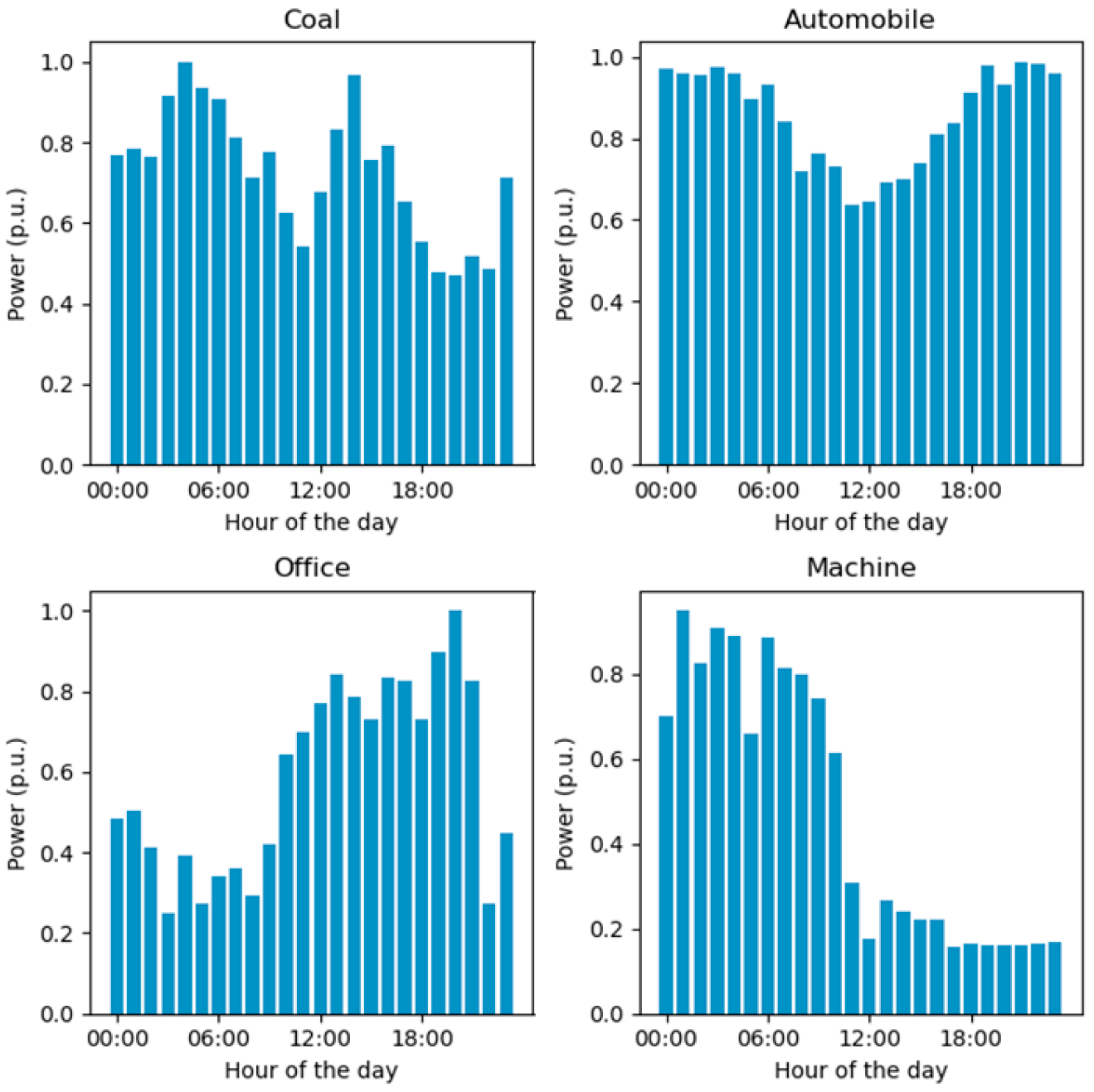
Eight kinds of consumers are chosen as the typical participants in the demand response and their baseline of power load are obtained from the actual measurements of representative users. We assume there are twelve loads with day-ahead flexibility from coal mines, automobile factories, office buildings, and machine manufacturers. There are also ten loads with intraday flexibility from commercial shopping malls, food industry, cement factories, and steel plants. As can be seen in Figure 2 and Figure 3, their normalized load profiles for each sector of consumers are shown as bar charts.

Figure 2.
Normalized load profile for load with day-ahead flexibility.
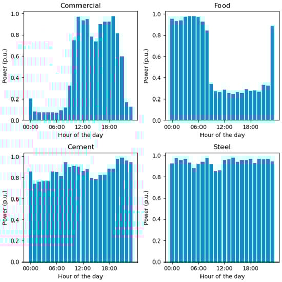
Figure 3.
Normalized load profile for load with intraday flexibility.
The day-ahead forecast of photovoltaic generation and total power-load baseline (including industrial and commercial loads participating in demand response and residential load) is illustrated in Figure 4. The PV generation exhibits a distinct diurnal pattern, with negligible generation during nighttime hours (00:00 to 06:00) and a rapid increase in generation starting from around 07:00. The generation peaks between 11:00 and 14:00, reaching values above 3.0 p.u., before gradually declining and tapering off completely by around 19:00. This pattern aligns with the expected behavior of solar generation, which depends on sunlight availability.
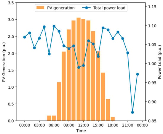
Figure 4.
Day-ahead forecast of photovoltaic generation and power load in the 141-bus system.
The total power load shows notable fluctuations throughout the day. There is a general trend of higher power load during the day compared to nighttime, with values ranging between 0.85 p.u. and 1.15 p.u. Unlike the PV generation, which has a clear peak, the power load displays multiple peaks and valleys, indicating varying demand patterns across different times of the day. A critical observation is the mismatch between the periods of peak PV generation and the highest power load. While PV generation peaks around noon, the power load does not perfectly align with this peak. There are periods during the day when the power load is relatively high, but PV generation is low (e.g., early morning and late evening). The discrepancy between the PV generation peak and the power load suggests significant potential for demand response strategies. By shifting some of the power load to the midday period when PV generation is at its highest, it is possible to increase the utilization of renewable energy and reduce reliance on conventional power sources. This load shifting can help balance the demand and supply, optimize energy usage, and reduce carbon emissions.
Another important observation is the high power load during the evening (around 18:00 to 21:00) when PV generation is almost zero. This evening peak represents a challenge as it typically requires additional power from non-renewable sources. Effective demand response strategies can target this peak, potentially shifting some of this load to times when renewable generation is available.
In summary, the day-ahead forecast reveals a typical PV generation profile with a strong midday peak and low generation during early morning and evening. The power load, however, is more evenly distributed throughout the day with multiple peaks. The analysis highlights the opportunity to implement demand response measures to shift power consumption to periods of high PV generation, thereby enhancing renewable energy utilization and contributing to a reduction in carbon emissions.
4.2. Analysis of Demand Response Schedule
In our numerical test, day-ahead demand response is carried out in advance. Afterward, we assume that the intraday forecast of photovoltaic generation after 7:00 slightly increases by a factor of 1.09 compared with its day-ahead forecast to reflect the influence of actual solar radiation. On the other hand, the actual response trajectory of loads with day-ahead flexibility is assumed to reach 85% of its day-ahead schedule due to their operational restrictions. Thus, based on the latest intraday forecast, the intraday demand response is invoked to adjust the schedule of load with intraday flexibility after 7:00 in a distributed manner.
Figure 5 illustrates the power-load baseline and the demand response schedules (day-ahead and intraday) for various loads with day-ahead demand response. The coal sector shows significant variability in its baseline load throughout the day, with peaks occurring around 05:00 and 10:00, and a notable drop around 15:00. The day-ahead demand response schedule generally follows the baseline pattern but smoothes the peaks and valleys. The automobile sector’s baseline load has peaks around 08:00 and 14:00, with a pronounced dip around 11:00. The day-ahead schedule slightly reduces the load during peak hours and increases it during the dip. For the office sector, the baseline load shows a morning peak around 09:00 and a steady rise toward a higher peak in the late afternoon. The day-ahead schedule effectively reduces the afternoon peak and shifts some of the load to earlier in the day. The machine sector exhibits a distinctive load profile with a significant peak around 06:00, which declines sharply by midday. The day-ahead schedule smoothes this peak and distributes the load more evenly across the morning and early afternoon.
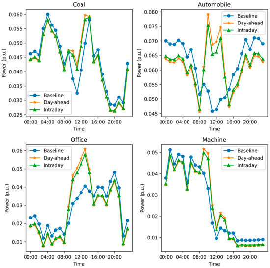
Figure 5.
The power-load baseline and the demand response schedules of load with day-ahead flexibility.
In general, the day-ahead scheduling phase successfully smoothes the load profiles across different sectors, reducing peaks and filling in valleys to better match the PV generation profile.
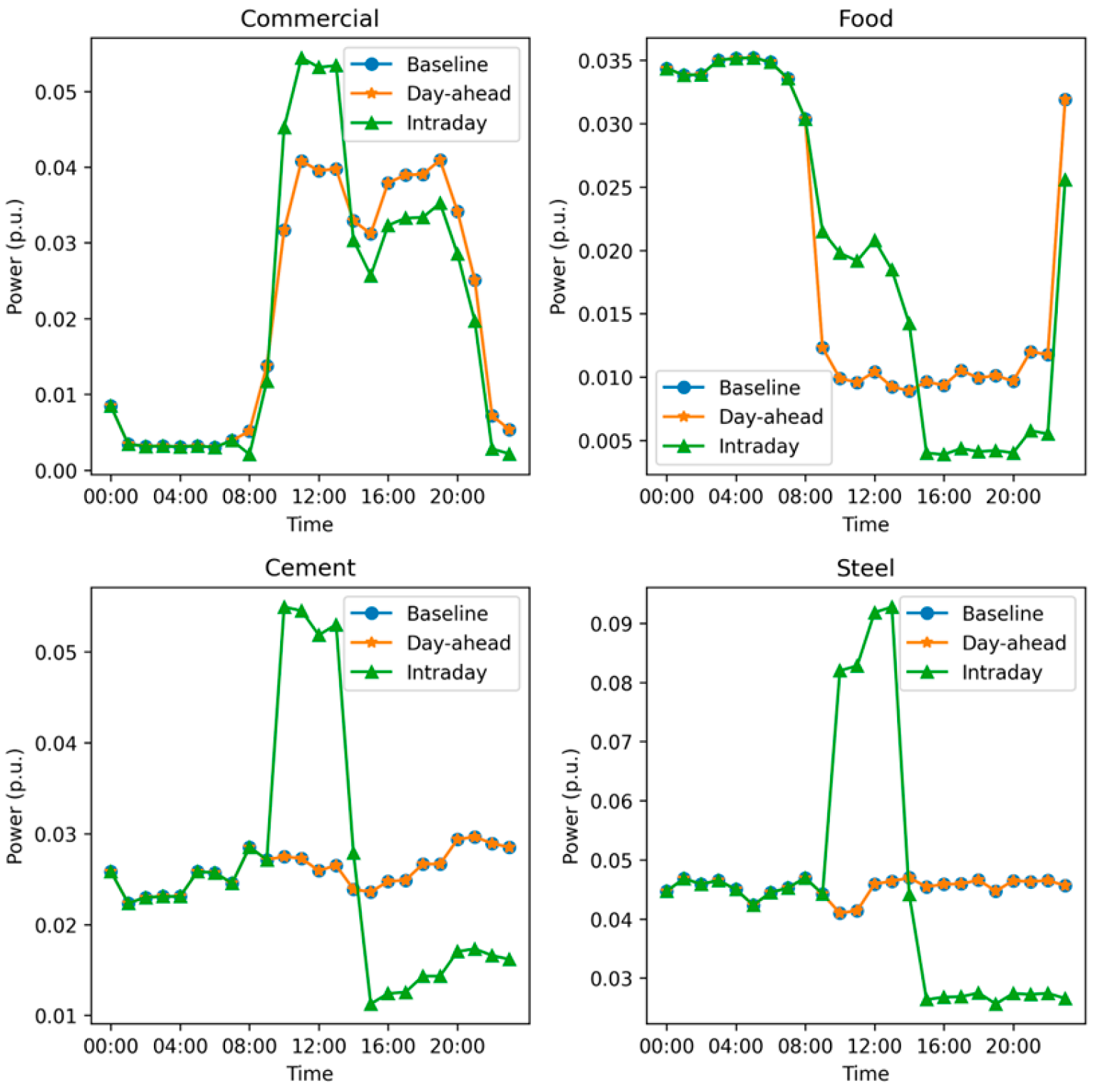
Figure 6 illustrates the power-load baseline and the demand response schedules for various loads with intraday demand response. The intraday adjustment is invoked at 7:00, but different loads have different response delays. The response delays are as follows: commercial (1 h), food (2 h), cement (3 h), and steel (3 h).
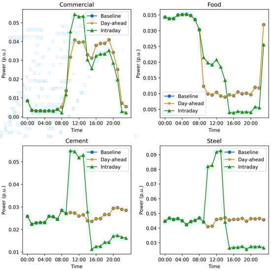
Figure 6.
The power-load baseline and the demand response schedules of load with intraday flexibility.
The commercial sector has a response delay of 1 h. The baseline load shows significant peaks around 10:00 and 15:00. The intraday adjustments, starting at 8:00, further optimize the load by reducing the peaks more effectively and spreading the load more evenly across the day. With a response delay of 2 h, the food sector’s baseline load shows a relatively high and consistent demand until a sharp drop at around 10:00, followed by a gradual decline and another peak at 20:00. The intraday adjustments starting at 9:00 significantly reduce the load during the midday peak and maintain a lower, more consistent load profile throughout the day.
The cement sector has a response delay of 3 h. The baseline load displays high demand in the early hours and another significant peak around 15:00. The intraday adjustments, starting at 10:00, show a drastic reduction in load during the peak hours and a more balanced distribution of load across the rest of the day, especially after the midday period. Also, with a 3 h response delay, the steel sector exhibits a high baseline load peak around 06:00 and maintains a relatively stable load throughout the day. The day-ahead schedule does not significantly alter this pattern. However, the intraday adjustments starting at 10:00 show a marked reduction in the peak load and a more consistent load profile for the remainder of the day, reflecting a significant adjustment to align with PV generation.
Figure 7 presents the power exchange with the transmission network under three scenarios: baseline (blue line), day-ahead schedule (orange line), and intraday adjusted schedule (green line), over a 24 h period. The baseline power exchange shows a typical daily pattern with high power imports from the transmission network during early morning and late evening hours, and significant power exports during midday. The highest imports occur between 00:00 and 06:00 and again from 17:00 to 22:00, reflecting the high power demand during these periods.
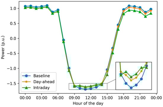
Figure 7.
The power exchange with the transmission network before and after day-ahead and intraday demand response.
The day-ahead demand response schedule shows a reduction in power imports during the morning peak hours and a smoother transition during the midday period. There is a noticeable flattening of the power exchange curve, indicating a more balanced distribution of power demand throughout the day. The power exports during midday are slightly reduced, suggesting a better alignment with the PV generation forecast. The total imported electricity quantity after day-ahead electricity decreases from 14.2 MWh to 7.9 MWh, which is equivalent to eliminating emission of 0.375 t CO2.
The intraday adjustments, which occur after 07:00, further optimize the power exchange pattern. These adjustments reduce the power imports more significantly during the morning and evening peaks and increase power exports during midday. This results in a more pronounced smoothing effect on the power exchange curve, particularly during the critical high-demand periods in the evening. The evening period, typically characterized by high power imports, shows a significant reduction in imports with both day-ahead and intraday demand response. This reduction is particularly noticeable between 17:00 and 22:00, suggesting that the demand response strategies effectively mitigate the evening peak load. The intraday adjustment further reduces the total imported electricity quantity from 7.9 MWh to 0.002 MWh, incurring additional reduction of 0.844 t CO2 emission.
Additionally, to account for the uncertainty in user load flexibility and the effectiveness of demand response, we established six scenarios in Appendix A, Table A1, to analyze system performance and carbon emissions reduction when load flexibility or participation rates are uncertain. The optimized analysis is detailed in Appendix A, Table A2: Comparing Scenarios I–III, as the flexibility of demand response loads increases, the reduction in carbon emissions gradually increases (total carbon emissions decrease). In Scenarios I and IV, as the flexibility of demand response load decreases within the day, the total carbon emissions show an upward trend. Additionally, we analyzed Scenarios V, I, and VI, where as the effectiveness of demand response improves within the day, the total carbon emissions also decrease accordingly.
Furthermore, for the DR model established in this study, in order to trade-off the carbon emissions and compensation costs, we used the ADMM algorithm to solve the carbon emission reduction corresponding to each compensation cost. Appendix A, Table A3, shows the optimization results considering the DR model trade-off analysis. It can be observed that when incorporating both the model-predicted carbon emissions and compensation costs, as compensation costs gradually increase, the reduction in carbon emissions progressively decreases, indicating a gradual rise in total carbon emissions.
The power exchange with the transmission network before and after the implementation of day-ahead and intraday demand response highlights the effectiveness of the proposed two-stage demand response mechanism. The day-ahead schedule initiates the optimization by smoothing the power exchange curve and reducing peak imports, while the intraday adjustments refine this optimization based on updated PV generation forecasts. The overall power exchange pattern becomes more balanced, with reduced reliance on the transmission network during peak hours and enhanced exports during midday. This balance contributes to more efficient energy management and better integration of renewable energy sources. The shift of power loads to align with PV generation periods is evident, indicating successful implementation of demand response strategies. This load shifting not only optimizes energy usage but also promotes sustainability by reducing carbon emissions associated with power imports. The demand response schedules also reflect sector-specific adjustments, accounting for different response delays and operational constraints. This tailored approach ensures that each sector contributes effectively to the overall optimization of the power exchange pattern.
In conclusion, the two-stage demand response mechanism significantly improves the power exchange with the transmission network, enhancing the utilization of renewable energy, reducing peak loads, and contributing to overall carbon emission reductions. The combined effect of day-ahead and intraday adjustments ensures a responsive and adaptive energy management strategy, capable of accommodating real-time changes in PV generation and demand patterns.
4.3. Analysis of Distributed Optimization Mechanism
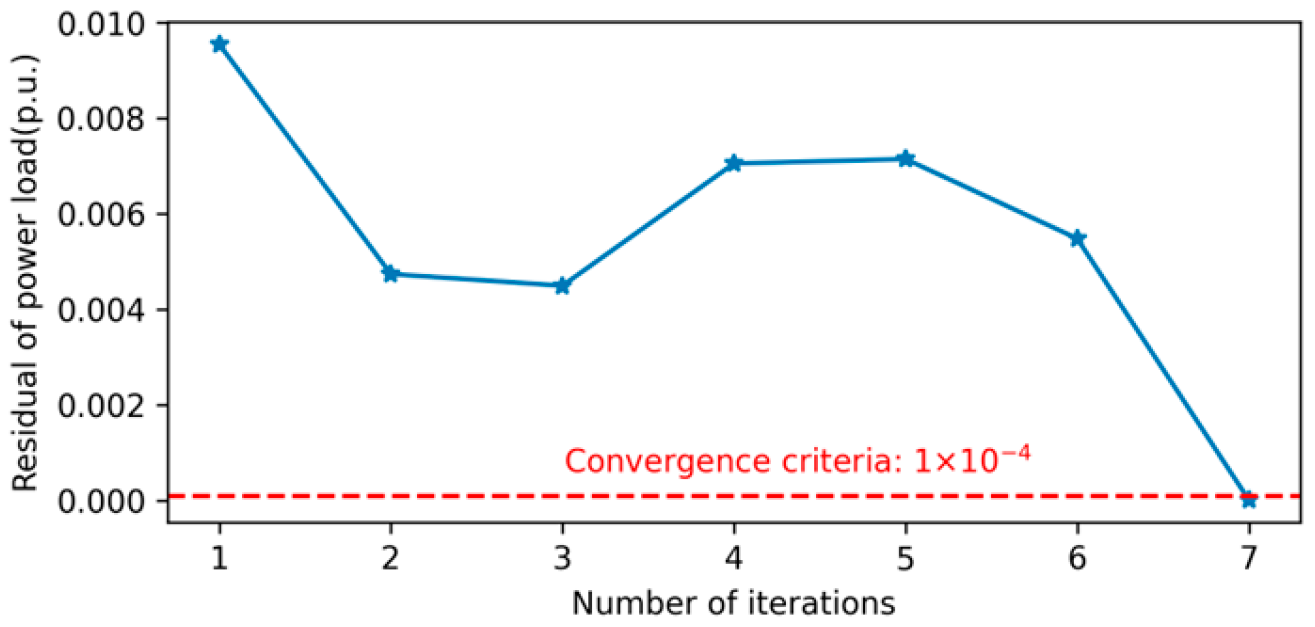
In our distributed demand response mechanism, we regard the difference between and as residuals indicating the convergence of optimization. The convergence criterion is selected as 1 × 10⁻⁴ p.u., which equals 1 kW.
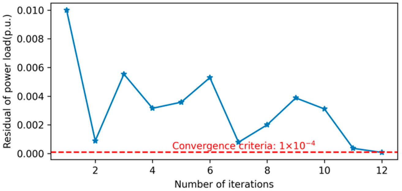
Figure 8 and Figure 9 show the change in residuals as the number of iterations increases when using the ADMM to solve the day-ahead and intraday demand response problem in a distributed manner. Appendix A, Table A4, shows the number of iterations, computation time, and convergence residual values. The final residual reaches close to zero after seven iterations and meets the convergence criterion of 1 × 10⁻⁴ p.u. for the day-ahead demand response problem. This indicates that the algorithm has successfully converged to an optimal solution within a reasonable number of iterations. The intraday demand response problem, although following a similar initial rapid convergence, exhibits more fluctuations between iterations 3 and 10, with residuals ranging from 0.002 p.u. to 0.005 p.u. Despite these fluctuations, the residuals eventually meet the convergence criterion of 1 × 10⁻⁴ p.u. by the twelfth iteration. The computation time for both day-ahead and intraday demand response is controlled within 2 s, indicating that even when communication delays or interruptions are taken into account in actual distributed deployments, this solution still has good real-time potential.
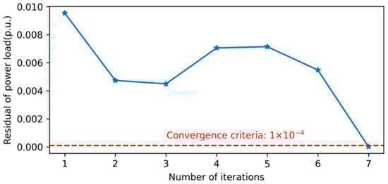
Figure 8.
Residual of power load in the global model and local model during iterations of day-ahead distributed demand response.
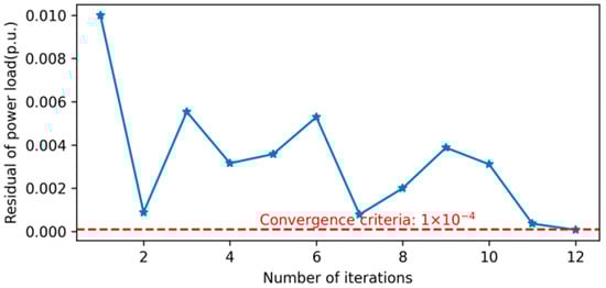
Figure 9.
Residual of power load in the global model and local model during iterations of intraday distributed demand response.
Overall, the ADMM algorithm proves to be effective for both day-ahead and intraday demand response problems, with rapid initial convergence and reliable final results, adapting well to the different complexities in each scenario.
5. Conclusions
This study proposes a distributed low-carbon demand response strategy that combines day-ahead and intraday flexibility, and uses the ADMM algorithm to solve distribution network scheduling optimization problems in a distributed manner. Through case study analysis, the effectiveness of the proposed strategy is verified, and the following conclusions are drawn:
- By implementing a distributed low-carbon demand response mechanism, we can effectively optimize power-load schedules to align with PV generation profiles, achieving source-load balance and reducing output fluctuations.
- Our approach combining day-ahead schedule and intraday adjustment successfully reduces evening peak loads and increases midday power consumption, thereby enhancing the utilization of local renewable energy and reducing the total carbon emission of distribution network. The day-ahead phase reduced CO2 emissions by 0.375 tons, and the intraday phase reduced CO2 emissions by 0.844 tons.
- The rapid convergence of the ADMM algorithm ensures the efficiency of the distributed demand response mechanism. In multiple operating scenarios, the total operating time of the system is less than 2 s. The results from the IEEE 141-bus test system validate the effectiveness of proposed demand response strategies and its ability to ensure low-carbon network operation.
However, this analysis lacks changes in carbon emission factors. In the future, we will fully consider the uncertainty of carbon emission factors, adopt uncertainty modeling methods for research, and analyze the number of iterations and computation time when verifying on a larger-scale system. This will enable further optimization of the load side, deeply explore the carbon reduction capabilities of distribution networks, and enhance their operational economic efficiency.
Author Contributions
Conceptualization, B.H.; methodology, Y.Y.; validation, B.H. and Y.Y.; writing—original draft preparation, X.Z. and Y.Y.; writing—review and editing, H.W. and Y.Y. All authors have read and agreed to the published version of the manuscript.
Funding
This work was supported by the Fundamental Research Funds for the Central Universities (JZ2025HGTA0155).
Data Availability Statement
The original contributions presented in the study are included in the article; further inquiries can be directed to the corresponding author.
Conflicts of Interest
The authors declare that the research was conducted in the absence of any commercial or financial relationships that could be construed as potential conflicts of interest.
Appendix A
Table A1.
Day-ahead and intraday flexibility scenarios.
Table A1.
Day-ahead and intraday flexibility scenarios.
| Scenario | Flexibility of Day-Ahead Demand Response | Flexibility of Intraday Demand Response | Day-Ahead Demand Response Result | ||
|---|---|---|---|---|---|
| Upward 2 | Downward | Upward | Downward | ||
| I | 40% | 32% | 100% | 60% | 0.85 |
| II 1 | 50% | 40% | 100% | 60% | 0.85 |
| III | 60% | 48% | 100% | 60% | 0.85 |
| IV | 50% | 40% | 80% | 40% | 0.85 |
| V | 50% | 40% | 100% | 60% | 0.7 |
| VI | 50% | 40% | 100% | 60% | 0.9 |
1 Represents the benchmark scenario for demand response flexibility and the effectiveness of day-ahead demand response implementation. 2 Represents the percentage of upward and downward adjustments compared to baseline load.
Table A2.
Day-ahead and intraday flexibility scenario optimization results.
Table A2.
Day-ahead and intraday flexibility scenario optimization results.
| Demand Response | Scenario | Carbon Emission Reduction (ton) | Iterations | Time (s) | Average time (s) |
|---|---|---|---|---|---|
| No DR | - | 0 | 1 | 0.090 | 0.090 |
| Day-Ahead Demand Response | I | 0.317 | 6 | 0.696 | 0.116 |
| II | 0.375 | 7 | 0.830 | 0.119 | |
| III | 0.434 | 8 | 0.987 | 0.123 | |
| IV | 0.375 | 7 | 0.859 | 0.123 | |
| V | 0.375 | 7 | 0.838 | 0.120 | |
| VI | 0.375 | 7 | 0.849 | 0.121 | |
| Intraday Demand Response | I | 0.797 | 13 | 1.011 | 0.078 |
| II | 0.844 | 12 | 0.907 | 0.076 | |
| III | 0.884 | 11 | 0.845 | 0.079 | |
| IV | 0.778 | 11 | 0.875 | 0.080 | |
| V | 0.811 | 20 | 1.508 | 0.075 | |
| VI | 0.868 | 20 | 1.624 | 0.081 |
Table A3.
Results of the trade-off analysis between carbon emissions and compensation costs.
Table A3.
Results of the trade-off analysis between carbon emissions and compensation costs.
| Scenario | Carbon Emission Reduction (ton) | Total Carbon Emission Reduction (ton) | |
|---|---|---|---|
| Day-Ahead | Intraday | ||
| Price reduced by 50% | 0.376116 | 0.845288 | 1.221404 |
| Base compensation price | 0.375444 | 0.844272 | 1.219716 |
| Price increased by 200% | 0.373622 | 0.845288 | 1.218910 |
| Price increased by 600% | 0.378142 | 0.837417 | 1.215559 |
Table A4.
Performance metrics computed on a day-ahead and intraday demand response.
Table A4.
Performance metrics computed on a day-ahead and intraday demand response.
| Performance Metrics | No Demand Response | Day-Ahead Demand Response | Intraday Demand Response |
|---|---|---|---|
| Number of Iterations | 1 | 7 | 12 |
| Total Time/s | 0.117 | 0.859 | 1.040 |
| Average time/s | 0.117 | 0.123 | 0.087 |
| Convergence Residual | 6.330 × 10⁻⁶ | 1.561 × 10⁻⁵ | 7.219 × 10⁻⁵ |
References
- Wang, Y.; Qiu, J.; Tao, Y. Optimal Power Scheduling Using Data-Driven Carbon Emission Flow Modelling for Carbon Intensity Control. IEEE Trans. Power Syst. 2022, 37, 2894–2905. [Google Scholar] [CrossRef]
- Wang, W.; Huang, S.; Zhang, G.; Liu, J.; Chen, Z. Optimal Operation of an Integrated Electricity-Heat Energy System Considering Flexible Resources Dispatch for Renewable Integration. J. Mod. Power Syst. Clean Energy 2021, 9, 699–710. [Google Scholar] [CrossRef]
- Hedayati-Mehdiabadi, M.; Hedman, K.W.; Zhang, J. Reserve Policy Optimization for Scheduling Wind Energy and Reserve. IEEE Trans. Power Syst. 2018, 33, 19–31. [Google Scholar] [CrossRef]
- Shi, J.; Guo, Y.; Tong, L.; Wu, W.; Sun, H. A Scenario-Oriented Approach to Energy-Reserve Joint Procurement and Pricing. IEEE Trans. Power Syst. 2023, 38, 411–426. [Google Scholar] [CrossRef]
- Brás, T.A.; Simoes, S.G.; Amorim, F.; Fortes, P. How Much Extreme Weather Events Have Affected European Power Generation in the Past Three Decades? Renew. Sustain. Energy Rev. 2023, 183, 113494. [Google Scholar] [CrossRef]
- Xiao, D.; Chen, H.; Cai, W.; Wei, C.; Zhao, Z. Integrated Risk Measurement and Control for Stochastic Energy Trading of a Wind Storage System in Electricity Markets. Prot. Control Mod. Power Syst. 2023, 8, 60. [Google Scholar] [CrossRef]
- Qian, L.; Lin, S.; Li, F.; Wang, W.; Li, D. Low Carbon Optimization Dispatching of Energy Intensive Industrial Park Based on Adaptive Stepped Demand Response Incentive Mechanism. Electr. Power Syst. Res. 2024, 233, 110504. [Google Scholar] [CrossRef]
- Luo, Y.; Hao, H.; Yang, D.; Zhou, B. Multi-Objective Optimization of Integrated Energy Systems Considering Ladder-Type Carbon Emission Trading and Refined Load Demand Response. J. Mod. Power Syst. Clean Energy 2024, 12, 828–839. [Google Scholar] [CrossRef]
- Kang, C.; Zhou, T.; Chen, Q.; Xu, Q.; Xia, Q.; Ji, Z. Carbon Emission Flow in Networks. Sci. Rep. 2012, 2, 479. [Google Scholar] [CrossRef]
- Chen, X.; Sun, A.; Shi, W.; Li, N. Carbon-Aware Optimal Power Flow. IEEE Trans. Power Syst. 2025, 40, 3090–3104. [Google Scholar] [CrossRef]
- Li, B.; Song, Y.; Hu, Z. Carbon Flow Tracing Method for Assessment of Demand Side Carbon Emissions Obligation. IEEE Trans. Sustain. Energy 2013, 4, 1100–1107. [Google Scholar] [CrossRef]
- Yang, L.; Luo, J.; Xu, Y.; Zhang, Z.; Dong, Z. A Distributed Dual Consensus ADMM Based on Partition for DC-DOPF With Carbon Emission Trading. IEEE Trans. Ind. Inform. 2020, 16, 1858–1872. [Google Scholar] [CrossRef]
- Ma, W.-J.; Wang, J.; Gupta, V.; Chen, C. Distributed Energy Management for Networked Microgrids Using Online ADMM With Regret. IEEE Trans. Smart Grid 2018, 9, 847–856. [Google Scholar] [CrossRef]
- Alowaifeer, M.; Alkhraijah, M.; Meliopoulos, A.P.S.; Grijalva, S. Grid Services Optimization From Multiple Microgrids. IEEE Trans. Smart Grid 2022, 13, 8–19. [Google Scholar] [CrossRef]
- Schwarz, S.; Monti, A. Computational Performance Study on the Alternating Direction Method of Multipliers Algorithm for a Demand Response Peak Shaving Application. IEEE Syst. J. 2023, 17, 3370–3381. [Google Scholar] [CrossRef]
- Dhamala, B.; Pokharel, K.; Karki, N.R. Dynamic Consensus-Based ADMM Strategy for Economic Dispatch with Demand Response in Power Grids. Electricity 2024, 5, 449–470. [Google Scholar] [CrossRef]
- Kou, W.; Park, S.-Y. A Distributed Energy Management Approach for Smart Campus Demand Response. IEEE J. Emerg. Sel. Top. Ind. Electron. 2023, 4, 339–347. [Google Scholar] [CrossRef]
- Rezaei, E.; Dagdougui, H.; Ojand, K. Hierarchical Distributed Energy Management Framework for Multiple Greenhouses Considering Demand Response. IEEE Trans. Sustain. Energy 2023, 14, 453–464. [Google Scholar] [CrossRef]
- Li, N.; Liu, W.; Wan, X.; Ren, X.; Yu, H. Day-Ahead and Intraday Economic Optimization Models of the Stackelberg Game Considering Source-Load Uncertainty. IEEE Access 2025, 13, 14344–14357. [Google Scholar] [CrossRef]
- Mansouri, S.A.; Nematbakhsh, E.; Ramos, A.; Tostado-Véliz, M.; Aguado, J.A.; Aghaei, J. A Robust ADMM-Enabled Optimization Framework for Decentralized Coordination of Microgrids. IEEE Trans. Ind. Inform. 2025, 21, 1479–1488. [Google Scholar] [CrossRef]
- Yang, J.; Yang, M.; Ma, K.; Dou, C.; Ma, T. Distributed Optimization of Integrated Energy System Considering Demand Response and Congestion Cost Allocation Mechanism. Int. J. Electr. Power Energy Syst. 2024, 157, 109865. [Google Scholar] [CrossRef]
- Shi, L.; Cen, Z.; Li, Y.; Wu, F.; Lin, K.; Yang, D. Distributed Optimization of Multi-Microgrid Integrated Energy System with Coordinated Control of Energy Storage and Carbon Emissions. Sustainability 2024, 16, 3225. [Google Scholar] [CrossRef]
- Chen, X.; Wu, G.; Long, Z.; Xiao, H.; Xu, L.; Ling, Q. Multi-time scale optimal dispatch of integrated energy systems considering source-load uncertainty and user-side demand response. J. Electr. Power Sci. Technol. 2024, 3, 217–227. [Google Scholar] [CrossRef]
- Mohajeryami, S.; Doostan, M.; Asadinejad, A.; Schwarz, P. Error Analysis of Customer Baseline Load (CBL) Calculation Methods for Residential Customers. IEEE Trans. Ind. Appl. 2017, 53, 5–14. [Google Scholar] [CrossRef]
- Chen, Y.; Xu, P.; Chu, Y.; Li, W.; Wu, Y.; Ni, L.; Bao, Y.; Wang, K. Short-Term Electrical Load Forecasting Using the Support Vector Regression (SVR) Model to Calculate the Demand Response Baseline for Office Buildings. Appl. Energy 2017, 195, 659–670. [Google Scholar] [CrossRef]
- Kong, X.; Wang, Z.; Xiao, F.; Bai, L. Power Load Forecasting Method Based on Demand Response Deviation Correction. Int. J. Electr. Power Energy Syst. 2023, 148, 109013. [Google Scholar] [CrossRef]
- Jiang, Y.; Gao, T.; Dai, Y.; Si, R.; Hao, J.; Zhang, J.; Gao, D.W. Very Short-Term Residential Load Forecasting Based on Deep-Autoformer. Appl. Energy 2022, 328, 120120. [Google Scholar] [CrossRef]
- Li, P.; Hu, Z.; Shen, Y.; Cheng, X.; Alhazmi, M. Short-Term Electricity Load Forecasting Based on Large Language Models and Weighted External Factor Optimization. Sustain. Energy Technol. Assess. 2025, 82, 104449. [Google Scholar] [CrossRef]
- Yang, Y.; Lin, C.; Xu, L.; Yang, X.; Wu, W.; Wang, B. Accelerating Optimal Power Flow With Structure-Aware Automatic Differentiation and Code Generation. IEEE Trans. Power Syst. 2025, 40, 1172–1175. [Google Scholar] [CrossRef]
- Khodr, H.M.; Olsina, F.G.; Jesus, P.M.D.O.-D.; Yusta, J.M. Maximum Savings Approach for Location and Sizing of Capacitors in Distribution Systems. Electr. Power Syst. Res. 2008, 78, 1192–1203. [Google Scholar] [CrossRef]


Disclaimer/Publisher’s Note: The statements, opinions and data contained in all publications are solely those of the individual author(s) and contributor(s) and not of MDPI and/or the editor(s). MDPI and/or the editor(s) disclaim responsibility for any injury to people or property resulting from any ideas, methods, instructions or products referred to in the content. |
© 2025 by the authors. Licensee MDPI, Basel, Switzerland. This article is an open access article distributed under the terms and conditions of the Creative Commons Attribution (CC BY) license (https://creativecommons.org/licenses/by/4.0/).