Robust Optimal Operation of Smart Microgrid Considering Source–Load Uncertainty

Abstract

The uncertainties arising from high renewable energy penetration on both the generation and demand sides pose significant challenges to distribution network security. Smart microgrids are considered an effective way to solve this problem. Existing studies exhibit limitations in prediction accuracy, Alternating Current (AC) power flow modeling, and integration with optimization frameworks. This paper proposes a closed-loop technical framework combining high-confidence interval prediction, second-order cone convex relaxation, and robust optimization to facilitate renewable energy integration in distribution networks via smart microgrid technology. First, a hybrid prediction model integrating Variational Mode Decomposition (VMD), Long Short-Term Memory (LSTM), and Quantile Regression (QR) is designed to extract multi-frequency characteristics of time-series data, generating adaptive prediction intervals that accommodate individualized decision-making preferences. Second, a second-order cone relaxation method transforms the AC power flow optimization problem into a mixed-integer second-order cone programming (MISOCP) model. Finally, a robust optimization method considering source–load uncertainties is developed. Case studies demonstrate that the proposed approach reduces prediction errors by 21.15%, decreases node voltage fluctuations by 16.71%, and reduces voltage deviation at maximum offset nodes by 17.36%. This framework significantly mitigates voltage violation risks in distribution networks with large-scale grid-connected photovoltaic systems.

1. Introduction

In the context of global climate change and the ongoing energy transition, renewable energy sources such as photovoltaic (PV) and wind power are being rapidly integrated into power systems [1]. However, their inherent volatility and uncontrollability pose significant challenges to power quality. On the one hand, PV systems, which consist entirely of power electronic devices, lack the inertial characteristics of conventional power sources. Their abrupt output fluctuations frequently impact grid frequency stability [2]. On the other hand, wind power exhibits anti-peak regulation behavior, generating lower output during peak load periods and higher output during off-peak periods. Furthermore, the large installed capacity of wind farms increases the risk of cascading failures upon disconnection [3]. The combined uncertainty of renewable energy output and rapidly growing load demand further complicates efforts to maintain supply–demand balance.

Distribution networks, as the critical infrastructure directly supporting load demand, are particularly affected. Urban core areas experience high daily load fluctuation ratios, while the integration of distributed PV systems frequently induces reverse power flow, escalating the risk of voltage violations. Traditional distribution network operation modes have approached their regulatory limits in terms of available adjustment margins [4]. Coordinating the impact of source–load uncertainties on distribution network operations has thus become an urgent priority. Smart microgrid technology, with its advanced capabilities in power forecasting, energy management, and collaborative control, can effectively mitigate renewable energy volatility, enable local consumption, and optimize scheduling. This approach addresses the stability, power quality, and operational control challenges posed by the high penetration of renewable energy in distribution grids. As such, smart microgrids represent a key enabling technology for the large-scale, reliable integration of renewable energy into distribution networks.

Existing smart microgrid studies primarily employ prediction techniques to quantify source–load uncertainties, which can be categorized into point prediction, probabilistic distribution prediction, and interval prediction [5,6,7]. Point prediction provides single-value forecasts for future output at specific timestamps. Abou Houran, et al. [8] achieved 95.71% accuracy in PV output prediction using Long Short-Term Memory (LSTM), while Al-Dahidi, et al. [9] improved prediction accuracy to 97.62% by integrating a Convolutional Neural Network with a Bayesian-optimized LSTM. However, the point forecast merely describes the fluctuation pattern of renewable energy output and load without analyzing their uncertainty, failing to provide a clear quantification of the uncertainty at each future time point [10]. Probabilistic distribution prediction enhances point prediction by incorporating error analysis. It constructs the probabilistic distribution of prediction errors by analyzing deviations between historical and predicted data, thereby forming a probabilistic forecast of future outputs [11]. Wang, et al. [12] used a back propagation neural network to predict the PV power in the distribution network and combined it with an empirical mode decomposition method to model the probability distribution of the multi-period error distribution, effectively quantifying source–load uncertainty. Nevertheless, this approach heavily depends on prior assumptions about prediction errors. When errors deviate from the assumed distribution, the predicted probability distribution may misrepresent reality [13], potentially leading to significant economic losses in decision-making. Interval prediction establishes confidence intervals through quantile points, which can remove the a priori assumptions and output credible prediction domains under different confidence levels directly based on statistical principles. A prediction interval provides a range within which the future value is expected to lie with a specified probability (confidence level) [14]. Research [14] utilized Variational Mode Decomposition (VMD) to extract the difference frequency characteristics of wind power generation data and designed different prediction models for wind power submodes with different frequency characteristics, thereby achieving the reliable prediction of wind power generation intervals. Massidda, et al. [15] demonstrated a 22.69% improvement in PV interval coverage using Quantile Regression with limited historical data. However, existing interval prediction methods overlook multi-frequency characteristics in source–load time-series data, limiting prediction accuracy. Therefore, this paper introduces multi-frequency features into the interval prediction technology of smart microgrids to achieve higher accuracy in predicting source–load uncertainty.

Scholars have conducted numerous studies on methods for handling uncertainty in smart microgrids. Stochastic optimization requires precise probability distributions and constructs optimal models under numerous uncertainty scenarios, but suffers from the curse of dimensionality [16,17]. In contrast, robust optimization employs uncertainty sets to describe variable fluctuations, offering enhanced reliability [18,19,20]. Robust optimization is a methodology that seeks solutions immune to uncertainty within predefined bounds (e.g., the prediction intervals), often by optimizing against the worst-case scenario within those bounds [21]. Wei, et al. [22] developed a distributed, robust optimization model for Direct Current (DC) power flow optimization under PV output uncertainty, deriving optimal dispatch schemes under worst-case scenarios. Study [23] introduces second-order cone relaxation techniques for solving AC power flow optimization problems in distribution networks. SOCR is a convexification technique that transforms nonconvex constraints into a solvable convex form. However, this paper ignored the issue caused by the uncertainty of PV output. Study [21] explored the impact of photovoltaic uncertainty on the planning of off-grid net-zero energy buildings. Jiang, et al. [24] summarized the constraints of each device in a smart microgrid and investigated the optimal robust scheduling problem. However, three limitations persist: (1) Existing studies predominantly reduce Alternating Current (AC) power flow to DC approximations, neglecting nonlinear AC characteristics. (2) Few studies have introduced robust optimization technology into smart microgrids to deal with source–load uncertainty while taking into account the AC characteristics of the distribution network. This limits their ability to resolve the distribution network node voltage over-limit problem caused by the widespread distributed photovoltaic (PV) integration to the distribution network. (3) Existing smart microgrid studies fail to exploit the synergistic interactions between prediction and optimization models, mostly considering only prediction or only optimization problems under given uncertainty scenarios, rather than fostering synergistic interactions.

Table 1. Literature review of optimal operation of smart grids.

Ref.	Renewable Energy Output Prediction				Distribution Network Optimization
	Point	Probabilistic Distribution	Interval	Multi-Frequency Features	AC	DC	Uncertainty
[5]	√	×	×	√	×	×	×
[6]	√	×	×	√	×	×	×
[7]	×	×	√	√	×	×	×
[8]	√	×	×	×	×	×	×
[9]	√	×	×	×	×	×	×
[10]	×	√	×	×	×	×	×
[11]	√	×	×	×	×	×	×
[12]	×	√	×	√	×	×	×
[13]	×	×	√	×	×	×	×
[14]	×	×	√	√	×	×	×
[15]	×	×	√	×	×	×	×
[16]	×	×	×	×	√	×	√
[17]	×	×	×	×	√	×	√
[18]	×	×	×	×	×	×	√
[19]	×	√	×	×	√	×	√
[20]	×	√	×	×	√	×	√
[21]	×	×	×	×	×	×	√
[22]	×	×	√	×	√	×	√
[23]	×	×	×	×	×	√	×
[24]	×	×	×	×	√	×	√
This paper	×	×	√	√	×	√	√

summarizes the focus of previous studies and highlights their shortcomings. To address these challenges, this paper establishes a closed-loop smart microgrid technical framework integrating high-precision uncertainty quantification, strictly convex AC power flow modeling, and robust optimization. The key contributions include: (1) Prediction phase: A three-tiered VMD-LSTM-Quantile Regression (QR) architecture is proposed, where VMD extracts multi-scale features from source–load time-series data, LSTM networks capture the long-short-term dependencies, and Quantile Regression derives credible prediction intervals under varying confidence levels. (2) Modeling phase: Breaking traditional linearization bottlenecks, a mixed-integer second-order cone programming (MISOCP) model is established via second-order cone relaxation (SOCR) to handle nonconvex AC power flow constraints. (3) Optimization phase: A robust optimization framework is constructed to achieve optimal decisions under source–load uncertainty intervals.

This paper contains a nomenclature table in the Nomenclature section, given the large number of abbreviations, variables, and parameters involved in this study. This paper constructs a complete technical roadmap in Figure 1. This framework integrates multi-frequency feature extraction based on VMD, time-series modeling based on LSTM, and interval prediction based on QR. It employs SOCR technology to achieve convex optimization modeling for AC power flow and ultimately addresses source–load uncertainty through robust optimization. The model solution relies on the MATLAB platform (version R2023a), utilizing the YALMIP toolbox(YALMIP Version: 2021.03.31) and GUROBI 9.5.2 solver for efficient computation. Notably, this study employs actual grid data from Dongguan City, China (19 June–18 July 2022, with 15 min resolution and 2880 time stamps) for validation, significantly enhancing the model’s engineering applicability. The structure of this paper is as follows: Section 2 details the materials and methods, including high-precision interval prediction, AC power flow convex relaxation modeling, and robust optimization framework; Section 3 presents the case study results and comparative analysis; Section 4 summarizes the conclusions.

2. Materials and Methods

2.1. High-Precision Interval Prediction Method: VMD-LSTM-Quantile Regression

2.1.1. Source–Load Data Multi-Frequency Feature Extraction: VMD

Variational Mode Decomposition (VMD) is an adaptive, non-recursive signal processing technique designed for preprocessing spatiotemporal sequence data. It decomposes the original signal into multiple Intrinsic Mode Functions (IMFs), which are reconstructed to separate multi-frequency features while filtering noise [25]. This approach not only reduces modal aliasing but also demonstrates enhanced noise robustness compared with traditional methods.

Given non-stationary power time-series data $x\left(t\right)$, VMD decomposes it into submodal sequences $u_k\left(t\right)$ with specific center frequencies and finite bandwidths as follows:

$$u_k\left(t\right)=A_k\left(t\right)cos\left({\varphi }_k\left(t\right)\right)$$

(1)

where $A_k\left(t\right)$ denotes the envelope amplitude of $u_k\left(t\right)$, and phase ${\varphi }_k\left(t\right)$ is a non-decreasing function, i.e., ${\varphi }_k^{\prime }\left(t\right)\ge 0$.

Each mode $u_k\left(t\right)$ is characterized by a center frequency and finite bandwidth. The variational problem is formulated to minimize the sum of estimated bandwidths for all modes:

The analytical signal of each modal component $u_k\left(t\right)$ is obtained through the Hilbert transform to obtain its unilateral spectral function, as follows:

$$\left[\delta \left(t\right)+{\displaystyle \frac{j}{\pi t}}\right]\cdot u_k\left(t\right)$$

(2)

where $\delta \left(t\right)$ represents the Dirac distribution.

Each decomposed mode corresponds to a frequency band. By modulating submodal frequencies to basebands using the predefined center frequencies $e^{-j{\omega }_{k}t}$ [3], as follows:

$$\left[\left(\delta \left(t\right)+{\displaystyle \frac{j}{\pi t}}\right)\cdot u_k\left(t\right)\right]e^{-j{\omega }_{k}t}$$

(3)

Bandwidth estimation for submodes incorporates L2-norm regularization to prevent overfitting, leading to the final variational formulation [3], as follows:

$$\underset{\left\{u_k\right\},\left\{{\omega }_k\right\}}{\min }\left\{{\displaystyle \sum }_k\parallel {\partial }_t\left[\left(\delta \left(t\right)+{\displaystyle \frac{j}{\pi t}}\right)\cdot u_k\left(t\right)\right]e^{-j{\omega }_{k}t}{\parallel }_2^2\right\}$$

(4)

$$s.t.{\displaystyle \sum }_k{u}_k\left(t\right)=x\left(t\right)$$

(5)

where $\left\{u_k\right\}=\left\{u_1,u_2,\dots ,u_K\right\}$ denotes the set of submodes, $\left\{{\omega }_k\right\}=\left\{{\omega }_1,{\omega }_2,\dots ,{\omega }_K\right\}$ represents center frequencies, and K is the number of submodes.

2.1.2. Time-Series Feature Prediction Technology: LSTM

The Long Short-Term Memory (LSTM) neural network is a specialized recurrent neural network architecture designed to retain long-term temporal dependencies through iterative learning, thereby enhancing prediction accuracy for sequential data [26]. Due to its chain-like unfolded structure, LSTM demonstrates superior performance in modeling temporal relationships.

For an input sequence with k time steps, the LSTM gate mechanism comprises forget, input, and output gates. $x_t$ carries the network input values introduced into the system as vectors, $h_t$ carries the outputs of the LSTM cells through the implicit layer, and $c_t$ carries the LSTM cell states for the operation. LSTM operations are defined as follows:

(1)

Compute the oblivious gate $f_t$ based on the hidden state $h_{t-1}$ at the previous moment and the input $x_t$ at the current moment [8], as follows:

$$f_t=\sigma \left(W_f{h}_{t-1}+U_f{x}_t+b_f\right)$$

(6)

where $W_f$, $U_f$ is the weight matrix, $b_f$ is the bias term, and $\sigma$ is the activation function (Sigmoid in this study).

(2)

The input gate $i_t$ is computed based on the hidden state $h_{t-1}$ at the previous moment and the input $x_t$ at the current moment [8], as follows:

$$i_t=\sigma \left(W_i{h}_{t-1}+U_i{x}_t+b_i\right)$$

(7)

(3)

The output gate $o_t$ is computed based on the hidden state $h_{t-1}$ at the previous moment and the input $x_t$ at the current moment [8], as follows:

$$o_t=\sigma \left(W_o{h}_{t-1}+U_o{x}_t+b_o\right)$$

(8)

where $W_o$, $U_o$ is the output gate weight matrix and $b_o$ is the bias term.

(4)

The tanh function is used as the activation function of the neuron to calculate the candidate memory cell ${\tilde{c}}_t$ based on the hidden state $h_{t-1}$ at the previous moment and the input $x_t$ at the current moment, as follows:

$${\tilde{c}}_t=tanh\left(W_c{h}_{t-1}+U_c{x}_t+b_c\right)$$

(9)

where $W_c$, $U_c$ is the memory gate weight matrix and $b_c$ is the bias term.

(5)

By combining the information about the memory cells of the previous moment and the candidate memory cells of the current moment, the flow of information is controlled by forgetting gates and input gates to compute the memory cells of the current moment $c_t$ [8], as follows:

$$c_t=f_t\odot c_{t-1}+i_t\odot {\tilde{c}}_t$$

(10)

(6)

Putting $c_t$ through the tanh activation function and the output gate, a new hidden state, i.e., the ultra-short-term prediction of distributed PV power, can be obtained as follows:

$$h_t=o_t\odot tanh\left(c_t\right)$$

(11)

(7)

After the aforementioned calculation, $c_t$ and $h_t$ are retained for the next time step; after the last step is completed, the hidden layer vector $h_k$ is used as the output to compare with the corresponding predicted value of this set of sequences to derive the value of the loss function, and based on the gradient descent algorithm, the optimization of the weights and bias parameters is performed, and the sum of squares error function is selected as the loss function of the LSTM as follows:

$$L={\displaystyle \frac{1}{2}}{\displaystyle \sum }_{i\in outputs}{\left({\widehat{y}}_i-y_i\right)}^2$$

(12)

2.1.3. Credible Uncertainty Interval Prediction Method: Quantile Regression

Quantile Regression (QR) effectively addresses the limitations of mean regression by providing a more comprehensive analysis of the relationship between independent and dependent variables. QR accurately characterizes how predictors influence the variation range in the response variable and captures their effects on the shape of the conditional distribution. Moreover, QR quantifies the impact of each input variable on the response variable across different quantile levels, thereby offering deeper insights into their underlying relationships [27]. The conditional quantile of the output response variable of the combined LSTM model is calculated as shown below:

$$S^{\left(\tau \right)}=f\left({\displaystyle \sum _{j=1}^J{w}_j\left(\tau \right)h_j\left(\tau \right)+b\left(\tau \right)}\right)$$

(13)

where $S^{\left(\tau \right)}$ represents the conditional quantile of the output response variable at the $\tau$ quantile, $w_j\left(\tau \right)$ represents the output layer weight, $h_j\left(\tau \right)$ represents the LSTM hidden layer output, $b\left(\tau \right)$ represents the output layer bias, and J represents the number of hidden layer units. After updating the network parameters, multiple LSTM models are generated with different weights and biases from each other. The explanatory variables are entered into the network and propagated forward to obtain the predicted values of the response variables, as shown in the following equation:

$$S_{t+h\left|t\right.}=\left\{S_{t+h\left|t\right.}^{\left({\tau }_1\right)},S_{t+h\left|t\right.}^{\left({\tau }_2\right)},\dots ,S_{t+h\left|t\right.}^{\left({\tau }_l\right)},\right\}$$

(14)

where $S_{t+h\left|t\right.}$ represents the group of response variable predicted values, $S_{t+h\left|t\right.}^{\left({\tau }_1\right)}$ represents the response variable predicted values at different moment quartiles, and l represents the number of LSTM networks at different quartiles.

2.2. AC Optimization Model for Smart Microgrids Based on Second-Order Cone Relaxation

2.2.1. AC Optimization Model for Smart Microgrids

Smart microgrids integrate PV, energy storage, and other distributed energy resources through advanced control technologies and optimization strategies. This integration enhances renewable energy utilization while maintaining system stability and reducing operational costs. To address the challenges posed by high renewable energy penetration in distribution networks, this section establishes an optimal scheduling model for smart microgrids.

(1)

Decision variables

The day-ahead optimal scheduling model for smart microgrids developed in this study aims to generate reliable and controllable scheduling plans based on predicted source–load output data at each node. The model’s decision variables encompass: (1) active and reactive power outputs of controllable equipment at 15 min intervals across a 24 h period, (2) nodal voltages, and (3) line currents, as formulated in Equation (15) as follows:

$$X=[P_G^i,Q_G^i,P_{PV}^i,P_{\mathrm{ES},\mathrm{c}}^i,P_{\mathrm{ES},\mathrm{d}}^i,V^i,I^j]$$

(15)

where $P_G^i$ and $Q_G^i$ refer to the active and reactive power of the distributed gas turbine. $P_{PV}^i$ refers to the active power of the distributed photovoltaic at node i, and $P_{\mathrm{ES},\mathrm{c}}^i$ and $P_{\mathrm{ES},\mathrm{d}}^i$ are the storage and discharge power of the distributed energy storage at node i, respectively. $V^i$ refers to the voltage at node i and $I^j$ refers to the current at line j.

(2)

Optimization objective

This study establishes a 24 h day-ahead optimal scheduling framework for smart microgrids with 15 min intervals. The model incorporates controllable distributed energy resources, including distributed generators, photovoltaic (PV) systems, and energy storage systems. Considering the relatively low cycling costs of energy storage, the economic objective function excludes storage regulation costs. To align with national energy policies, the model prioritizes high PV utilization by penalizing power curtailment. Additionally, the model accounts for network loss costs, as current flow through transmission lines generates power losses that may affect power quality.

In summary, the optimization objective of the day-ahead smart microgrid is shown in Equation (16) as follows:

$$\left\{\begin{array}{c}F=\underset{X}{\min }{\displaystyle \sum _{t=1}^T\left[{\displaystyle \sum _{i\in N_{node}}\left(C_G^{i,t}+C_{PV}^{i,t}\right)}+{\displaystyle \sum _{i,j\in N_{line}}{C}_{Loss}^{ij,t}}\right]}\\ C_G^{i,t}={\mu }_{\mathrm{G}}^i{P}_{\mathrm{G}}^{i,t}\Delta t\\ C_{PV}^{i,t}={\mu }_{PV}^i{P}_{PV,curt}^i\Delta t\\ C_{Loss}^{ij,t}=={\mu }_{\mathrm{Loss}}{I}_{ij}^2{r}_{ij}\Delta t\end{array}\right.$$

(16)

where $N_{node}$ refers to the set of nodes in the distribution network. $N_{line}$ refers to the set of lines in the distribution network, T is the set of optimal scheduling time periods, $C_G^{i,t}$ refers to the operating cost of distributed gas turbines in the distribution network at node i in time t, $C_{PV}^{i,t}$ refers to the penalty cost of photovoltaic power curtailment in the distribution network, and $C_{Loss}^{ij,t}$ refers to the cost of network loss of the line ij in the smart microgrid in time period t. ${\mu }_{\mathrm{G}}$ refers to the cost of distributed gas turbines per unit of generated power, ${\mu }_{PV}$ refers to the cost of distributed PV per unit of discarded power penalty, ${\mu }_{\mathrm{Loss}}$ refers to the cost incurred per unit of line loss, $I_{ij,t}$ refers to the current flowing through the line ij in time period t, and $r_{ij}$ is the magnitude of the resistance of the line ij.

(3)

Model constraints

The constraints in the smart microgrid trend optimization model include distributed gas turbine output constraints, distributed PV output constraints, distributed energy storage output constraints, and tidal current constraints.

The distributed gas turbine output should not exceed its allowable range, and the constraints are shown in Equation (17) as follows:

$$\left\{\begin{array}{c}0\le P_G^i\le P_{G,\max }^i\\ Q_{G,\min }^i\le Q_G^i\le Q_{G,\max }^i\end{array}\right.$$

(17)

where $P_{G,\max }^i$ and $Q_{G,\max }^i$ refer to the upper limit of active and reactive power of the distributed gas turbine at node i, and $Q_{G,\min }^i$ refers to the lower limit of reactive power of the distributed gas turbine at node i.

In this study, the impact of distributed PV in the distribution network is mainly considered, and it is considered that distributed PV adopts the maximum power point tracking (MPPT) control model. Distributed PV power output is limited by installed capacity and light resources, and its power output model is shown in Equation (18) [21] as follows:

$$\left\{\begin{array}{c}0\le P_{PV}^i\le P_{PV,unit}^i{W}_{PV}^i\\ P_{PV,curt}^i=P_{PV,unit}^i{C}_{PV}^i-P_{PV}^i\end{array}\right.$$

(18)

where $P_{PV}^i$ and $P_{PV,curt}^i$ are the active and abandoned power of distributed PV at node i, $W_{PV}^i$ refers to the installed capacity of distributed PV at node i, and $P_{PV,unit}^i$ refers to the scalar value of distributed PV output, which is affected by real-time light resources.

Distributed energy storage, on the other hand, is modeled based on the charge state, as shown in Equation (19) [28]. The model incorporates three key coordination mechanisms for battery dispatch under uncertainty: (1) Temporal coordination through state-of-charge constraints (Equation (19)A–C) that enforce energy conservation across the optimization horizon while maintaining sufficient capacity reserves for worst-case scenarios. (2) Power coordination via complementary charging/discharging constraints (Equation (19)D–F) that prevent simultaneous operations and ensure feasible power transitions. (3) Adaptive coordination through net discharge power definition (Equation (19)G) that enables dynamic response to renewable generation fluctuations within the predicted uncertainty bounds. This integrated approach automatically achieves optimal battery dispatch by balancing immediate power needs with long-term energy availability requirements under uncertainty.

$$\left\{\begin{array}{cc}{S}_{\mathrm{ES}}^{i,t}=\left(P_{\mathrm{ES},\mathrm{c}}^{i,t}{\eta }_{\mathrm{ES},\mathrm{c}}-P_{\mathrm{ES},\mathrm{d}}^{i,t}/{\eta }_{\mathrm{ES},\mathrm{d}}\right)+\left(1-{\gamma }_{\mathrm{ES}}\right)S_{\mathrm{ES}}^{i,t-1}& (19\mathrm{A})\\ S_{\min }^{\mathrm{ES}}\le S_{\mathrm{ES}}^{i,t}\le S_{\max }^{\mathrm{ES}}& (19\mathrm{B})\\ S_{\mathrm{ES}}^{i,0}=S_{\mathrm{ES}}^{i,T}& (19\mathrm{C})\\ 0\le P_{\mathrm{ES},\mathrm{c}}^{i,t}\le u_{\mathrm{ES},\mathrm{c}}^{i,t}{\tau }_{\mathrm{ES}}{W}_{\mathrm{ES}}^i& (19\mathrm{D})\\ 0\le P_{\mathrm{ES},\mathrm{d}}^{i,t}\le u_{\mathrm{ES},\mathrm{d}}^{i,t}{\tau }_{\mathrm{ES}}{W}_{\mathrm{ES}}^i& (19\mathrm{E})\\ q_{\mathrm{ES},\mathrm{c}}^{i,t}+q_{\mathrm{ES},\mathrm{d}}^{i,t}\le 1& (19\mathrm{F})\\ P_{\mathrm{ES}}^{i,t}=P_{\mathrm{ES},\mathrm{d}}^{i,t}-P_{\mathrm{ES},\mathrm{c}}^{i,t}& (19\mathrm{G})\end{array}\right.$$

(19)

where $S_{\mathrm{ES}}^{i,t}$ is the remaining storage power of the distributed energy storage at node i at time point t, $P_{\mathrm{ES},\mathrm{c}}^{i,t}$ and $P_{\mathrm{ES},\mathrm{d}}^{i,t}$ are the charging power and discharging power of the distributed energy storage at node i at time point t, ${\eta }_{\mathrm{ES},\mathrm{c}}$ and ${\eta }_{\mathrm{ES},\mathrm{d}}$ refer to the charging and discharging efficiencies of this type of distributed energy storage, and ${\gamma }_{\mathrm{ES}}$ stands for the self-discharging rate of this battery, and T is the total step length of the planning cycle, and in the day-ahead optimal scheduling model, the total optimization cycle is 24 h with a 15-step length, i.e., T = 96. $S_{\min }^{\mathrm{ES}}$ and $S_{\max }^{\mathrm{ES}}$ refer to the lower and upper limits of battery storage; $q_{\mathrm{ES},\mathrm{c}}^{i,t}$ and $q_{\mathrm{ES},\mathrm{d}}^{i,t}$ refer to the charging and discharging labels of the distributed energy storage at node i at moment t. $P_{\mathrm{ES}}^{i,t}$ refers to the net discharge power of the distributed storage at node i at moment t. When it is greater than zero, it means that the battery is being discharged at that moment, and vice versa for charging.

AC power flow constraints are the most fundamental constraints for a smart microgrid. The conventional tidal current equations are nonlinear, nonconvex equational constraints that contain trigonometric functions in addition to the product term, as shown below [23]:

$$P_{Gi}-P_{Li}-U_i{\displaystyle {\sum }_{j=1}^N{U}_j\left(G_{ij}\cos {\theta }_{ij}+B_{ij}\sin {\theta }_{ij}\right)}=0$$

(20)

$$Q_{Gi}-Q_{Li}-U_i{\displaystyle {\sum }_{j=1}^N{U}_j\left(G_{ij}\sin {\theta }_{ij}-B_{ij}\cos {\theta }_{ij}\right)}=0$$

(21)

$$P_G^{\min }\le P_{Gi}\le P_G^{\max }$$

(22)

$$Q_G^{\min }\le Q_{Gi}\le Q_G^{\max }$$

(23)

$$U^{\min }\le U_i\le U^{\max }$$

(24)

$$S_l^{\min }\le S_{li}\le S_l^{\max }$$

(25)

where $P_{Gi}$ and $Q_{Gi}$ represent the active and reactive power from generators (including gas turbines and PV units) at node i, respectively; $P_{Li}$ and $Q_{Li}$ are the active and reactive power consumed by the load at the node, respectively; $B_{ij}$ and $G_{ij}$ represent the conductance and conductivity between branch ij; $U_i$ and ${\theta }_{ij}$ represent the voltage amplitude at the node and the phase difference of the voltage at the node ij; $S_{li}$ represents the power flowing over the ith branch, $S_l^{\max }$ and $S_l^{\min }$ represent the upper and lower limit values of the branch currents; $P_G^{\max }$, $P_G^{\min }$, $Q_G^{\max }$, and $Q_G^{\min }$ represent the upper and lower limits of active and reactive generator output; $U^{\max }$ and $U^{\min }$ denote the upper and lower limits of the node voltage within the safe range.

2.2.2. Accurate Convex Relaxation Method Based on Mixed-Integer Second-Order Cone

Due to the AC constraints (Equations (20)–(25)), the optimal dispatch model for the constructed microgrid is a nonlinear and nonconvex optimization problem. To ensure the solvability of the model, this paper introduces the second-order cone relaxation technique to transform the model into a convex optimization problem. The specific steps are as follows:

The DistFlow model is introduced to describe the power flow constraints [23], as shown in Figure 2.

Under this model, Equations (20) and (21) are transformed into Ohm’s law constraints, branch head end power equation constraints, and node power balance equation constraints as follows:

$$V_i-V_j=Z_{ij}{I}_{ij}$$

(26)

$${\tilde{S}}_{ij}=V_i{\overline{I}}_{ij}$$

(27)

$${\displaystyle {\sum }_{k:j\to k}{S}_{jk}}-{\displaystyle {\sum }_{i:i\to j}\left(S_{ij}-Z_{ij}{\left|I_{ij}\right|}^2\right)}=S_j$$

(28)

where $I_{ij}$ is the current flowing through branch ij, $Z_{ij}$ is the impedance of line ij, $V_i$ refers to the voltage at node i, ${\overline{I}}_{ij}$ refers to the conjugate of $I_{ij}$, $S_{jk}$ refers to the power flowing out of node j to node k, and $S_j$ refers to the power injected by the external unit at node j.

In the above model, $S_{ij}$, $I_{ij}$, $V_i$, and $S_j$ all contain both magnitude and phase angle, so phase relaxation is required. Let $l_{ij}={\left|I_{ij}\right|}^2$, $v_i={\left|V_i\right|}^2$ and split Equation (28) into active and reactive forms as follows:

$${\displaystyle {\sum }_{k:j\to k}{P}_{jk}}-{\displaystyle {\sum }_{i:i\to j}\left(P_{ij}-r_{ij}{l}_{ij}\right)}=P_j$$

(29)

$${\displaystyle {\sum }_{k:j\to k}{Q}_{jk}}-{\displaystyle {\sum }_{i:i\to j}\left(Q_{ij}-x_{ij}{l}_{ij}\right)}=Q_j$$

(30)

This can be obtained by bringing Equation (27) into Equation (26), followed by the squaring operation:

$$v_j=v_i-2\left(r_{ij}{P}_{ij}+x_{ij}{Q}_{ij}\right)+\left(r_{ij}^2+x_{ij}^2\right)l_{ij}$$

(31)

where $r_{ij}$ refers to the resistance of line ij and $x_{ij}$ refers to the reactance of line ij.

Similarly, squaring Equation (27) yields:

$$l_{ij}{v}_i=P_{ij}^2+Q_{ij}^2$$

(32)

Now, the AC power flow constraint no longer contains complex variables; however, Equation (27) is still a nonconvex constraint. In order to turn it into a convex constraint, a second-order cone relaxation method is introduced, as shown in Equation (28), which turns it into a rotating second-order cone, relaxes the original decision domain into a convex domain, and ensures that the optimal solution still falls on the original decision domain.

$$l_{ij}{v}_i\ge P_{ij}^2+Q_{ij}^2$$

(33)

2.3. Robust Optimal Dispatch Model for Smart Microgrid Considering AC and Source–Load Bilateral Uncertainty

2.3.1. Robust Optimization Techniques for Smart Microgrid Considering Decision Makers’ Individualized Decision Preferences

In this paper, a novel optimization framework is proposed to determine the confidence level based on the decision maker’s individualized decision preference. On this basis, the source–load uncertainty interval under a given confidence level is obtained by combining prediction techniques and integrating these intervals into a robust optimization model to produce scenario-adaptive solutions. The key to the framework lies in how to interface the decision preferences with the robust optimization model through the prediction technique. The details are as follows:

Robust optimization addresses uncertainties in renewable generation and load demand to maintain system feasibility across all operational scenarios. However, existing robust optimization approaches for smart microgrids typically employ fixed uncertainty intervals without leveraging probabilistic distribution information from interval predictions, often yielding overly conservative solutions. This study proposes a novel optimization framework that incorporates decision-makers’ risk preferences to determine appropriate confidence levels. The framework combines these preferences with advanced prediction techniques to derive source–load uncertainty intervals at specified confidence levels, which are then integrated into the robust optimization model to generate scenario-adaptive solutions. The core innovation involves effectively interfacing decision preferences with the optimization model through predictive analytics, as detailed below:

First, an acceptable level of confidence $\xi$ is obtained based on the decision maker’s preferences.

Second, the uncertainty faced by the smart microgrid studied in this paper mainly includes the uncertainty of distributed PV output and the uncertainty of electricity load at each node. Combining the given confidence level $\xi$ with the VMD-LSTM-QR technique described in the previous section, to obtain the source–load uncertainty interval under this confidence level. At this point, the uncertainty variables can be defined as follows:

$$\left\{\begin{array}{c}U=[P_{\mathrm{PV},unit}^{i,t},P_{\mathrm{Load}}^{i,t},Q_{\mathrm{Load}}^{i,t}]\\ \mathrm{Pr}\left\{P_{\mathrm{PV},unit}^{i,t,\min }\le P_{\mathrm{PV},unit}^{i,t}\le P_{\mathrm{PV},unit}^{i,t,\max }\right\}\ge {\xi }_1\\ \mathrm{Pr}\left\{P_{\mathrm{Load}}^{i,t,\min }\le P_{\mathrm{Load}}^{i,t}\le P_{\mathrm{Load}}^{i,t,\max }\right\}\ge {\xi }_2\\ \mathrm{Pr}\left\{Q_{\mathrm{Load}}^{i,t,\min }\le Q_{\mathrm{Load}}^{i,t}\le Q_{\mathrm{Load}}^{i,t,\max }\right\}\ge {\xi }_3\end{array}\right.$$

(34)

where $P_{\mathrm{PV},unit}^{i,t,\min }$ and $P_{\mathrm{PV},unit}^{i,t,\max }$ are the upper and lower bounds of the predicted PV output specification at a confidence level of ${\xi }_1$; $P_{\mathrm{Load}}^{i,t,\min }$ and $P_{\mathrm{Load}}^{i,t,\max }$ are the upper and lower bounds of the predicted active load of electricity consumption at each node at a confidence level of ${\xi }_2$; $Q_{\mathrm{Load}}^{i,t,\min }$ and $Q_{\mathrm{Load}}^{i,t,\max }$ are the upper and lower bounds of the predicted reactive load of electricity consumption at each node at a confidence level of ${\xi }_3$; $\mathrm{Pr}$ refers to the probability.

Finally, robust optimization proves particularly effective in addressing distribution network scheduling challenges under significant source–load bilateral uncertainties. This approach enhances system security and operational stability by explicitly considering worst-case scenarios. Based on the AC optimal power flow model presented in the previous section, the robust optimization model for smart microgrids is constructed as follows:

$$\left\{\begin{array}{c}\underset{X}{\min }\underset{U}{\max }{\displaystyle \sum _{t=1}^T\left[{\displaystyle \sum _{i\in N_{node}}\left(C_G^{i,t}+C_{PV}^{i,t}\right)}+{\displaystyle \sum _{i,j\in N_{line}}{C}_{Loss}^{ij,t}}\right]}\\ s.t. \mathrm{Device} \mathrm{constraints}: Equations \left(18\right) and \left(19\right)\\ \mathrm{Power} \mathrm{flow} \mathrm{constraints}: Equations(22)–(25),Equations(29)–(33)\\ \mathrm{Uncertainty} \mathrm{variable} \mathrm{constraint}: Equation(34)\end{array}\right.$$

(35)

2.3.2. Solving Method Based on Strong Duality Principle

The day-ahead robust optimization scheduling model constructed in this paper is a nonlinear and nonconvex optimization problem. In order to ensure the solvability of the model, this paper adopts the second-order cone relaxation technique to transform the model into a nonlinear convex optimization problem, which is specifically detailed in Section 2.2. After the processing, the compact expression of the model is shown in Equation (36), and the model is a two-layer nonlinear convex optimization problem. The inner-layer max function makes the worst performance of the microgrid economics objective by searching for the worst scenario $\tilde{u}$ within $\Omega \left(U,\xi \right)$, and the outer-layer min function minimizes the total operating cost of the distribution network under the worst scenario $\tilde{u}$ by optimizing the decision variable X.

$$\left\{\begin{array}{c}\underset{X}{\min }\underset{U}{\max }F\\ s.t.\left\{\begin{array}{c}Ax\le B\\ Cx=D+\tilde{u}\\ \tilde{u}\in \Omega \left(U,\xi \right),x\in \Omega \left(x\right)\end{array}\right.\end{array}\right.$$

(36)

where A, B, C, and D are constant coefficient matrices, $\tilde{u}$ refers to the uncertainty variable in a scenario, $\Omega \left(U,\xi \right)$ refers to the uncertainty range of the uncertainty variable $\tilde{u}$ at confidence level $\xi$, and $\Omega \left(x\right)$ refers to the decision domain of the decision variable.

The min–max form of Equation (36) makes it still not directly solvable. Since it is a convex optimization problem with zero dual gap, the optimal solution of the dyadic problem is equal to the optimal solution of the original problem. Further, this paper derives Equation (36) to its dyadic form based on strong duality theory, as shown in Equation (37):

$$\left\{\begin{array}{c}\underset{u,\alpha ,\beta }{\max }{\tilde{u}}^T\alpha +D^T\alpha +B^{\top }\beta \\ s.t.\left\{\begin{array}{c}\kappa +C^T\alpha +A^T\beta =c\\ \beta ⩽0\\ \kappa \in {\Omega }_k\\ \tilde{u}\in \Omega \left(U,\xi \right)\end{array}\right.\end{array}\right.$$

(37)

where $\alpha$, $\beta$, and $\kappa$ are dyadic variables and ${\Omega }_k$ refers to the dyadic space.

However, both $\tilde{u}$ and $\alpha$ are variables in Equation (37), which makes the model take the form of bilinear convex optimization, so the large M method is further used to deal with the bilinear term, as shown in Equation (38):

$$\left\{\begin{array}{c}\underset{u,\alpha ,\beta ,\nu }{\max }{D}^T\alpha +B^{\top }\beta +{\underset{¯}{u}}^{\mathrm{T}}\alpha +{\overline{u}}^{\mathrm{T}}\widehat{\alpha }-{\underset{¯}{u}}^{\mathrm{T}}\widehat{\alpha }\\ s.t.\left\{\begin{array}{c}\kappa +C^T\alpha +A^T\beta =c\\ \beta \le 0,\kappa \in {\Omega }_k,\tilde{u}\in \Omega \left(U,\xi \right)\\ -{\nu }_{t}M\le {\widehat{\alpha }}_t\le {\nu }_{i}M\\ {\alpha }_t-\left(1-{\nu }_t\right)M\le {\widehat{\alpha }}_t\le {\alpha }_t+\left(1-{\nu }_t\right)M\end{array}\right.\end{array}\right.$$

(38)

where M is a very large real number; $\widehat{\alpha }$ is an auxiliary variable; ${\widehat{\alpha }}_t$ is the component of $\widehat{\alpha }$ on time period t; ${\nu }_t$ is a zero-one variable introduced for $\widehat{\alpha }$. When ${\nu }_t$ = 1, ${\widehat{\alpha }}_t=\alpha$ and $u$ obtains the upper limit $\overline{u}$ in the interval $\Omega \left(U,\xi \right)$; when ${\nu }_t$ = 0, ${\widehat{\alpha }}_t=0$ and $u$ obtains the lower limit $u$ in the interval $\Omega \left(U,\xi \right)$. At this point, the model has been transformed into a mixed-integer second-order cone convex optimization problem, and the optimal solution can be obtained by the solver.

3. Results and Discussion

3.1. Calculation Background

In order to verify the superiority of the closed-loop smart microgrid technology of high-precision uncertainty quantification–strict convex modeling–robust optimization proposed in this paper, the adjusted IEEE33 node model is used for case study analysis. The IEEE 33-bus system was selected as it is a widely adopted and extensively studied standard benchmark for medium-voltage distribution networks. Its established topology and parameters facilitate direct comparison of results (e.g., computational efficiency, voltage profiles, and SOCR accuracy [23]) with numerous existing studies in the field, enhancing the credibility and reproducibility of our findings. The adjusted node system is shown in Figure 3.

It is worth noting that the method described in this paper is not only applicable to the current asset allocation and node system: (1) Greater node system adaptability: in the technical framework proposed in this paper, the algorithms in the prediction component are independent of the node system. The DistFlow method, which models AC power flow as a convex quadratic cone model, has also been proven to be applicable to larger node systems [29]. Similarly, equipment constraints and uncertainty constraints are also independent of the node system. Therefore, the proposed method can be extended to larger systems after appropriate power flow modeling and adjustments; (2) Asset mix flexibility: The optimization model employs modular device constraints. This allows seamless integration of diverse assets by modifying only device-specific parameters while preserving the core AC-RO framework. Regulatory constraints (e.g., voltage limits ± 7%) are embedded as generic safety bounds (Equation (24)), ensuring adaptability to regional standards.

The test system comprises a 33-node distribution network, with node 33 serving as the reference voltage node to ensure power flow compatibility with external grid connections. The system employs 12.66 kV as the base voltage with ±7% allowable voltage fluctuation and 1 MVA as the reference power. Line parameters follow the specifications in reference [30]. The network integrates distributed PV systems with capacities of 1600 kW at nodes 6, 24, and 32, and 2400 kW at node 17. Node 33 hosts a 5 MW gas turbine with active power output limits of 0–100% and reactive power limits of −20% to 60%. Energy storage systems (1200 kWh/2 h each) are deployed at nodes 15 and 28, utilizing lithium-ion batteries with state-of-charge limits of 5–95% and 97% charge/discharge efficiency. Battery self-discharge is negligible for the day-ahead optimization horizon. The model incorporates the following cost parameters: gas turbine generation at 0.15 CNY/kWh, a PV curtailment penalty at 0.25 CNY/kWh, and a network loss penalty at 0.2 CNY/kWh.

This paper sets up multiple comparative scenarios to verify the effectiveness of the aforementioned method. The specific scenarios are set up in

Table 2. Settings of Forecasting Methods and Optimization Approaches for Different Scenarios.

Scenario	Prediction Methods	Optimization Method
S1	LSTM	-
S2	ARIMA	-
S3	VMD-LSTM-QR	-
S4	VMD-LSTM-QR	Deterministic optimization
S5	VMD-LSTM-QR	Robust optimization

.

3.2. Results of the Application of High-Precision Interval Prediction Algorithms

3.2.1. Data Sources

Distributed PV output and nodal load data of the microgrid come from a region in Dongguan City, China, and the recorded time period is from 19 June 2022 to 18 July 2022, with a 15 min interval and a total of 2880 timestamps. The distributed PV and nodal load data are shown in Figure 4 after normalization. Among them, 80% of these data are used as the training set for LSTM, and 20% of these data are used as the test set for LSTM. In this paper, there is no difference between the prediction process of distributed PV and nodal load, and in order to save space, the prediction results of nodal load are used as the object of analysis. A brief comparison of the distributed photovoltaic prediction results under different methods is shown in Appendix A.

3.2.2. Evaluation Indicators

In order to verify the prediction effect of the VMD-LSTM model proposed in this paper, it is tested against the LSTM model via simulation. The mean squared error (MSE), root mean square error (RMSE), mean absolute error (MAE), and prediction interval coverage probability (PICP) are chosen as the evaluation indexes.

MSE is the mean of the sum of squares of the differences between the real and predicted values at the corresponding points. The smaller the value of MSE, the better the fit of the model [6].

$$e_{MSE}={\displaystyle \frac{{{\displaystyle \sum }}_{m=1}^M{\left(w_{m,true}-w_{m,pred}\right)}^2}{M}}$$

(39)

where M is the sample size; $w_{m,true}$ is the true value; $w_{m,pred}$ is the predicted value; $m$ is the number.

RMSE is the square root of the ratio of the square of the deviation of the predicted value from the true value to the sample size, which is more sensitive to outliers in the data. The smaller the RMSE value, the better the model prediction [6].

$$e_{RMSE}=\sqrt{e_{MSE}}$$

(40)

MAE refers to the mean absolute error, which represents the average of the absolute errors between the predicted values and the observed values [6].

$$e_{MAE}={\displaystyle \frac{{{\displaystyle \sum }}_{m=1}^M\left|w_{m,true}-w_{m,pred}\right|}{M}}$$

(41)

PICP refers to the prediction interval coverage probability, which reflects the probability that the actual observed value falls within the upper and lower bounds of the prediction interval [14].

$$PICP={\displaystyle \frac{{{\displaystyle \sum }}_{m=1}^M{k}_m}{M}}$$

(42)

where $k_m$ is a Boolean value. If the predicted target value is included in the upper and lower limits of the interval prediction, then $k_m$ = 1; otherwise, $k_m$ = 0.

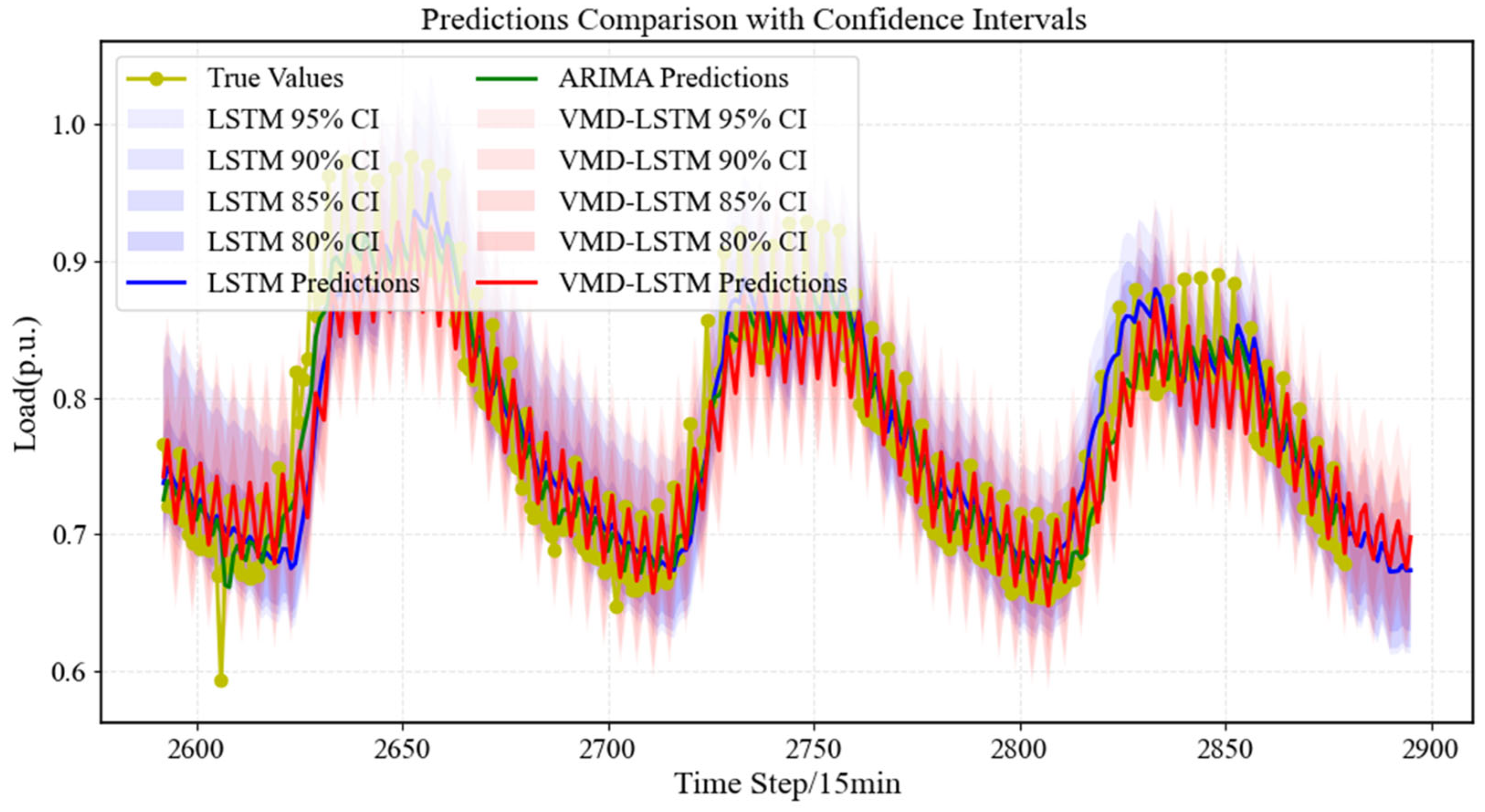
3.2.3. Predicted Results

When making predictions, the VMD-LSTM model and the LSTM model were compared separately in order to show more clearly the accuracy of the VMD-LSTM model in prediction, and then the predicted values were plotted along with the real load values. In addition, to demonstrate the predictive ability of the models, the loads were predicted in steps of 15 min. Finally, the obtained predicted values are output in the form of confidence intervals of predicted values with probabilities based on the Quantile Regression model. Based on the VMD processing of data, the obtained difference frequency characteristics are shown in Figure 5. In Figure 5, IMF1 represents the long-term frequency characteristics, IMF2 represents the short-term frequency characteristics, and the sum of IMF1 and IMF2 is approximately equal to the original signal (i.e., the original load time-series data). The deviation is caused by the influence of high-frequency noise. Based on this, the VMD-LSTM-QR prediction results, the traditional LSTM prediction results, and the traditional ARIMA prediction results are shown in Figure 6, and the comparison of the performance of the evaluation indexes of the three algorithms is shown in

Table 3. Comparison of results of forecasting models.

Indicators	LSTM (S1)	ARIMA (S2)	VMD-LSTM-QR (S3)	Precision Improvement (Mean)
MSE	10.57 × 10−3	14.17 × 10−3	6.79 × 10−3	39.38%
	74.59%	100%	47.92%
RMSE	102.79 × 10−3	107.64 × 10−3	82.45 × 10−3	21.15%
	95.49%	100%	76.60%
MAE	36.51 × 10−3	31.36 × 10−3	25.77 × 10−3	22.36%
	100%	85.89%	70.58%
PICP	-		84.21% (90% CI)	-

.

We conducted experiments on the prediction part using a CPU on a computer platform. The computing environment was as follows: 12th Gen Intel (R) Core (TM) i7-12700, 32 GB RAM. The times taken by the traditional algorithm (LSTM) and the method proposed in this paper (VMD-LSTM-QR) were 56.78 s and 176.39 s, respectively. Since VMD-LSTM-QR needs to analyze and predict each frequency feature, it consumes more computing resources and time. However, compared with its prediction time scale (prediction of output and load for the next 24 h), it only takes a few minutes, so it does not affect its application value. From the comparative analysis of the prediction results in Table 3 and the prediction curves in Figure 6, it can be seen that the VMD-LSTM-QR model proposed in this paper significantly reduces the MSE and RMSE and exhibits good prediction results compared with the LSTM method only. Compared with the LSTM model, the prediction model proposed in this paper reduces the MSE, RMSE, and MAE by 39.38%, 21.15%, and 22.36%, respectively, with a high prediction accuracy of 91.75%. Therefore, the VMD-LSTM model proposed in this paper can effectively extract the high-dimensional features in the time-series and map them to the low-dimensional space by combining the VMD variational modal decomposition technique, extracting different frequency features from the load data, and predicting them individually, which enhances the ability of the LSTM model in capturing the complex dynamic relationship of the time-series and thus improves the prediction accuracy. In addition, at a 90% confidence level, the PICP of the proposed uncertainty interval prediction model is as high as 84.21%. The model proposed in this paper can provide prediction intervals with a confidence level through Quantile Regression, which greatly enhances the reliability of the prediction results.

3.3. Robust Optimization Results for Active Distribution Networks Considering Source–Load Uncertainty

3.3.1. Basic Data

In order to make the scheduling results closer to reality, this paper increases the node load models in IEEE 33 from one to four. Nodes 1–8, nodes 9–17, nodes 18–24, and nodes 25–32 belong to four load behavior models, respectively. When using the traditional point prediction model, the future four distributed PV output power and four load behavior prediction results in this region are shown in Figure 7. A confidence level of 80% is determined based on the decision maker’s preference, and combined with the source–load uncertainty interval prediction method described in the previous section, the source–load uncertainty intervals for the region are obtained as shown in Figure 8 and Figure 9. The solid lines in Figure 8 and Figure 9 represent the values obtained by the point prediction method, while the shaded areas correspond to the uncertainty intervals obtained by the interval prediction method described in this paper. It is not difficult to see that the method described in this paper captures the inherent variability of solar power generation and load. During periods of high variability (such as sunrise/sunset or cloud cover events), wider bands of photovoltaic output are typically observed.

3.3.2. Model Robustness Validation

In order to verify the superiority of the proposed day-ahead robust planning optimization economic dispatch model and the effectiveness of the proposed robust optimization solution method, two scenarios of deterministic optimization and uncertainty optimization are set up for comparison in this paper. In the deterministic optimization, the distributed PV generation output and nodal electricity load are adopted as the values in Figure 7; in the uncertainty optimization, the distributed PV generation output and nodal electricity load are adopted as the intervals in Figure 8 and Figure 9. A comparison of costs under the robust optimization scheduling scheme and the deterministic optimization scheduling scheme is shown in

Table 4. Cost comparison between robust and deterministic optimization.

	Gas Turbine Costs (CNY)	PV Abandonment Penalties (CNY)	Network Loss Cost (CNY)	Total Cost (CNY)
Deterministic optimization (S3)	6681.8749	0	215.8463	6897.7212
Robust optimization (S4)	7427.5819	0	231.2719	7658.8538
Incremental share	10.04%	0%	6.67%	9.94%

. The functional flow balances under the two scheduling schemes are shown in Figure 10, the real-time voltages at each node for the whole day are shown in Figure 11, the current pairs of each line are shown in Figure 12, and the two distributed energy storage scheduling strategies are shown in Figure 13.

The total operating cost of the microgrid obtained by the robust optimal scheduling strategy (CNY 7658.85) is higher than that obtained by deterministic optimal scheduling (CNY 6897.72), representing an increase of approximately 9.94%. This increase stems primarily from higher gas turbine generation costs (increased by 10.04%) and network loss costs (increased by 6.67%), as detailed in Table 4. This cost difference arises because robust optimization explicitly considers worst-case scenarios within the predicted uncertainty intervals (95% confidence level in this case). Under these adverse conditions, which are characterized by potentially increased loads and lower active output from renewable sources, the system relies more heavily on dispatchable gas turbines to meet demand, leading to higher fuel costs. Concurrently, the altered power flow patterns under these scenarios result in increased resistive losses on the network lines. The cost components are calculated based on the following unit costs: gas turbine generation at 0.15 CNY/kWh, a PV curtailment penalty at 0.25 CNY/kWh (though no curtailment occurred in these scenarios), and a network loss penalty at 0.20 CNY/kWh. While robust optimization incurs a higher operational cost under nominal conditions, its key benefit lies in significantly enhancing operational reliability under uncertainty. Observing Figure 11 and Figure 12, it is evident that the robust optimization strategy ensures voltage and power flow fluctuations remain within stable and acceptable ranges even when subjected to uncertain renewable power output and load shocks. Specifically, robust optimization results in more uniform current and voltage distributions compared with deterministic optimization, effectively mitigating the specific high current and voltage peaks observed under deterministic conditions. This reduces the risk of thermal overload on lines and transformers. Critically, robust optimization ensures strict voltage compliance within the allowable ±7% deviation limits across all nodes and time periods, eliminating the risk of voltage violations observed in deterministic schedules under adverse scenarios (e.g., reducing the maximum voltage deviation at node 17 by 17.36%).

To evaluate the advantages of the proposed uncertainty-optimized scheduling scheme in handling intermittent renewable energy variability and to compare robust optimization with deterministic approaches, we analyze three key metrics: (1) the gas turbine’s active power output (representing the largest share of total active output), (2) nodal voltages during peak PV generation (12:00, when voltage deviation is maximum), and (3) hourly line currents (focusing on line 1 with the highest current), as illustrated in Figure 14.

As can be seen from Figure 14, the gas turbine output has a high degree of trend identity with the current of line 1. The gas turbine in the robust optimization sends out more active power in order to cope with the uncertain power loading scenario to ensure that the loads at each node can be adequately satisfied even after considering the uncertainty. In addition, by analyzing the time period with the largest voltage shift in the distribution network (12:00) and comparing the voltage at each node in the distribution network at this time, it is not difficult to find that the robust economic optimization scheduling method proposed in this paper is able to reduce the voltage fluctuation of the node (node 17) by about 16.71% and the voltage shift of the node (node 17) with the largest voltage shift of the entire microgrid by about 17.36%.

Notably, deterministic scheduling may lead to voltage violations during periods of high PV generation, potentially compromising system security. Our uncertainty optimization method significantly reduces the probability of such violations, consistently maintaining both voltage and line current within safe operating limits throughout all periods. These improvements facilitate greater integration of renewable energy sources into distribution networks.

In summary, the proposed closed-loop smart microgrid framework not only enhances operational efficiency and reliability but also offers valuable insights for grid planners and regulators. By providing a robust tool for uncertainty quantification and optimization, the model facilitates more informed decision-making regarding the integration of renewable energy sources into distribution grids. This approach can aid in the strategic placement and sizing of renewable assets, ensuring that grid expansion and reinforcement efforts are aligned with both technical capabilities and policy objectives. Ultimately, the framework supports the broader goal of promoting sustainable energy practices while maintaining grid stability and security.

3.3.3. Trade-Off Analysis Between Reliability and Cost of the Solution

This section presents a sensitivity analysis that quantifies the relationship between solution reliability (robustness against uncertainty) and operational cost. Reliability is governed by the confidence interval $\xi$ of the source–load uncertainty sets (Section 2.3.1), reflecting the decision-maker’s risk tolerance. Higher $\xi$ values widen the uncertainty intervals, enhancing system security but increasing conservatism and cost.

As depicted in Figure 15, the total cost exhibits a nonlinear increase with $\xi$. At $\xi =80\%$, the cost is CNY 7500 (baseline deterministic: CNY 6898). Increasing reliability to $\xi =90\%$ raises costs to CNY 9215 (+25.14% vs. deterministic), while $\xi =95\%$ incurs CNY 10,047. The marginal cost curve reveals a critical inflection point at $\xi =90\%$. Below this threshold, each 1% reliability gain costs approximately CNY 160; beyond it, costs surge to CNY 170–180 per 1%, indicating diminishing returns. Finally, we suggest selecting the $\xi =90\%$ solution as the optimal trade-off using the elbow method, which is often used in the process of selecting the number of clusters.

3.3.4. Validation of the Effectiveness of the Second-Order Cone Convex Relaxation Strategy

In order to verify the accuracy of the proposed model, the second-order cone error indicator ${\Delta }_{ij,t}=\left|P_{ij,t}^2+Q_{ij,t}^2-{\mathit{U}}_{i,t}{\overline{\mathit{I}}}_{ij,t}\right|$ is defined, where $P_{ij,t}$ and $Q_{ij,t}$ are the active and reactive power flowing from node i to node j in the branch ij, respectively. ${\overline{\mathit{I}}}_{ij,t}$ is the conjugate form of the currents on line ij containing the phase angle obtained by derivation. ${\mathit{U}}_{i,t}$ refers to the form of the voltage phasor at node i at the time t. Figure 16 is a plot of the current error check of the second-order cone relaxation optimization at each node every 15 min, and the overall error in index order of magnitude is controlled at 10⁻³ order of magnitude, which can meet the practical application requirements.

4. Conclusions

This study establishes a closed-loop smart microgrid framework integrating three core innovations: (1) High-precision interval prediction via a VMD-LSTM-QR architecture, enabling adaptive uncertainty quantification with multi-scale feature extraction. (2) Convex AC optimization modeling through second-order cone relaxation, overcoming traditional DC approximation limitations while ensuring computational tractability. (3) Robust decision-making that bridges prediction intervals with operational preferences, enhancing resilience against source–load uncertainties. Validation using real-world Dongguan grid data demonstrates a 21.15% prediction error reduction, 16.71% voltage fluctuation mitigation, and 17.36% decrease in maximum voltage deviation. These improvements directly address critical challenges in distribution networks with high-penetration renewables, notably reducing overvoltage risks during distributed PV integration, detailed as follows:

(1)

Significant Improvement in Prediction Accuracy: Compared with the traditional LSTM model, the combined prediction architecture based on VMD, LSTM, and QR proposed in this paper is able to effectively extract the difference frequency features in the time-series, improve the ability of the LSTM model to capture the complex dynamic relationships in the time-series, and reduce the prediction error by 21.15%.

(2)

Model Accuracy Enhancement: Traditional models mostly use DCs, and the resulting scheme is difficult to adapt to the distribution network operation under the impact of large-scale distributed PV. In this paper, a second-order cone relaxation strategy is used to control the AC power flow errors to 10⁻³ orders of magnitude, which verifies the rigor of the convex relaxation process and meets the practical application requirements.

(3)

System Robustness Enhancement: The robust decision of the microgrid at the 95% confidence level results in an increase of 10.04% in the total operating cost but manifests itself as a significant improvement in key safety parameters. Voltage fluctuations in the microgrid are reduced by 16.71%, and the largest voltage offset is reduced by about 17.36%, which significantly reduces the voltage over-limit risk in the distribution network under large-scale distributed PV shocks.

The framework proposed in this paper provides grid operators with a deployable toolkit for enhancing operational security amid renewable variability. By converting uncertainty into actionable confidence intervals, it supports policy goals for distributed energy integration without requiring structural grid upgrades. Future work will extend this approach to multi-microgrid coordination and hydrogen storage synergy, while specifically incorporating demand response flexibility to better leverage consumer-side resources in balancing supply–demand variations. Additionally, we will explore advanced uncertainty quantification methods such as distributionally robust optimization to further bridge the gap between stochastic and robust paradigms, with particular attention to how demand-side management interacts with these optimization frameworks.

References

1. Haoxin, D.; Qiyuan, D.; Chaojie, L.; Nian, L.; Zhang, W.; Hu, M.; Xu, C. A comprehensive review on renewable power-to-green hydrogen-to-power systems: Green hydrogen production, transportation, storage, re-electrification and safety. Appl. Energy 2025, 390, 125821. [Google Scholar] [CrossRef]
2. Useche-Arteaga, M.; Gil-González, W.; Gomis-Bellmunt, O.; Cheah-Mane, M.; Lacerda, V. Robust energy management in active distribution networks using mixed-integer convex optimization. Electr. Power Syst. Res. 2024, 241, 111367. [Google Scholar] [CrossRef]
3. Zhang, G.; Xu, B.; Liu, H.; Hou, J.; Zhang, J. Wind Power Prediction Based on Variational Mode Decomposition and Feature Selection. J. Mod. Power Syst. Clean Energy 2021, 9, 1520–1529. [Google Scholar] [CrossRef]
4. Li, G.; Wang, W.; Pang, D.; Wang, Z.; Tan, W.; Wang, Z.; Ge, J. A cloud-edge collaborative optimization control strategy for voltage in distribution networks with PV stations. Int. J. Electr. Power Energy Syst. 2025, 167, 110632. [Google Scholar] [CrossRef]
5. Ouyang, J.; Zuo, Z.; Wang, Q.; Duan, Q.; Zhu, X.; Zhang, Y. Seasonal distribution analysis and short-term PV power prediction method based on decomposition optimization Deep-Autoformer. Renew. Energy 2025, 246, 122903. [Google Scholar] [CrossRef]
6. Peng, S.; Zhu, J.; Wu, T.; Yuan, C.; Cang, J.; Zhang, K.; Pecht, M. Prediction of wind and PV power by fusing the multi-stage feature extraction and a PSO-BiLSTM model. Energy 2024, 298, 131345. [Google Scholar] [CrossRef]
7. Wang, L.; Mao, M.; Xie, J.; Liao, Z.; Zhang, H.; Li, H. Accurate solar PV power prediction interval method based on frequency-domain decomposition and LSTM model. Energy 2023, 262, 125592. [Google Scholar] [CrossRef]
8. Abou Houran, M.; Bukhari, S.M.; Zafar, M.H.; Mansoor, M.; Chen, W. COA-CNN-LSTM: Coati optimization algorithm-based hybrid deep learning model for PV/wind power forecasting in smart grid applications. Appl. Energy 2023, 349, 121638. [Google Scholar] [CrossRef]
9. Al-Dahidi, S.; Alrbai, M.; Rinchi, B.; Alahmer, H.; Al-Ghussain, L.; Hayajneh, H.S.; Alahmer, A. Techno-economic implications and cost of forecasting errors in solar PV power production using optimized deep learning models. Energy 2025, 323, 135877. [Google Scholar] [CrossRef]
10. Riedel, P.; Belkilani, K.; Reichert, M.; Heilscher, G.; von Schwerin, R. Enhancing PV feed-in power forecasting through federated learning with differential privacy using LSTM and GRU. Energy AI 2024, 18, 100452. [Google Scholar] [CrossRef]
11. Dong, H.; Shan, Z.; Zhou, J.; Xu, C.; Chen, W. Refined modeling and co-optimization of electric-hydrogen-thermal-gas integrated energy system with hybrid energy storage. Appl. Energy 2023, 351, 121834. [Google Scholar] [CrossRef]
12. Wang, S.; Sun, Y.; Zhang, S.; Zhou, Y.; Hou, D.; Wang, J. Very short-term probabilistic prediction of PV based on multi-period error distribution. Electr. Power Syst. Res. 2023, 214, 108817. [Google Scholar] [CrossRef]
13. Qiu, L.; Ma, W.; Feng, X.; Dai, J.; Dong, Y.; Duan, J.; Chen, B. A hybrid PV cluster power prediction model using BLS with GMCC and error correction via RVM considering an improved statistical upscaling technique. Appl. Energy 2024, 359, 122719. [Google Scholar] [CrossRef]
14. Tang, G.; Wu, Y.; Li, C.; Wong, P.K.; Xiao, Z.; An, X. A Novel Wind Speed Interval Prediction Based on Error Prediction Method. IEEE Trans. Ind. Inform. 2020, 16, 6806–6815. [Google Scholar] [CrossRef]
15. Massidda, L.; Bettio, F.; Marrocu, M. Probabilistic day-ahead prediction of PV generation. A comparative analysis of forecasting methodologies and of the factors influencing accuracy. Sol. Energy 2024, 271, 112422. [Google Scholar] [CrossRef]
16. Yi, T.; Li, Q.; Zhu, Y.; Shan, Z.; Ye, H.; Xu, C.; Dong, H. A hierarchical co-optimal planning framework for microgrid considering hydrogen energy storage and demand-side flexibilities. J. Energy Storage 2024, 84, 110940. [Google Scholar] [CrossRef]
17. Wang, S.; Hou, Y.; Guan, X.; Liu, S.; Huo, Z. Resiliency-informed optimal scheduling of smart distribution network with urban distributed photovoltaic: A stochastic P-robust optimization. Energy 2024, 313, 133449. [Google Scholar] [CrossRef]
18. Nasiri, N.; Zeynali, S.; Ravadanegh, S.N.; Kubler, S.; Le Traon, Y. A convex multi-objective distributionally robust optimization for embedded electricity and natural gas distribution networks under smart electric vehicle fleets. J. Clean. Prod. 2023, 434, 139843. [Google Scholar] [CrossRef]
19. Jodeiri-Seyedian, S.-S.; Fakour, A.; Nourollahi, R.; Zare, K.; Mohammadi-Ivatloo, B.; Zadeh, S.G. Nodal pricing of renewable-oriented distribution network in the presence of EV charging stations: A hybrid robust/stochastic optimization. J. Energy Storage 2023, 70, 107943. [Google Scholar] [CrossRef]
20. Li, P.; Wu, Z.; Yin, M.; Shen, J.; Qin, Y. Distributed data-driven distributionally robust Volt/Var control for distribution network via an accelerated alternating optimization procedure. Energy Rep. 2023, 9, 532–539. [Google Scholar] [CrossRef]
21. Li, G.; Xu, X.; Cheng, X.; Wang, Q.; Zhang, Y.; Wu, H.; Liu, D. Robust configuration planning for net zero-energy buildings considering source-load dual uncertainty and hybrid energy storage system. Build. Environ. 2025, 282, 113239. [Google Scholar] [CrossRef]
22. Wei, Z.; Xu, H.; Chen, S.; Sun, G.; Zhou, Y. Learning-aided distributionally robust optimization of DC distribution network with buildings to the grid. Sustain. Cities Soc. 2024, 113, 105649. [Google Scholar] [CrossRef]
23. Gholami, K.; Azizivahed, A.; Li, L.; Zhang, J. Accuracy enhancement of second-order cone relaxation for AC optimal power flow via linear mapping. Electr. Power Syst. Res. 2022, 212, 108646. [Google Scholar] [CrossRef]
24. Jiang, Z.; Yu, Q.; Xiong, Y.; Li, L.; Liu, Y. Regional active distribution network planning study based on robust optimization. Energy Rep. 2021, 7, 314–319. [Google Scholar] [CrossRef]
25. Udenze, P.I.; Gong, J.; Soltani, S.; Li, D. A deep neural network with two-step decomposition technique for predicting ultra-short-term solar power and electrical load. Appl. Energy 2024, 382, 125212. [Google Scholar] [CrossRef]
26. Yang, C.; Li, S.; Gou, Z. Spatiotemporal prediction of urban building rooftop photovoltaic potential based on GCN-LSTM. Energy Build. 2025, 334, 115522. [Google Scholar] [CrossRef]
27. Hu, Y.; Deng, X.; Yang, L. Interval prediction model for residential daily carbon dioxide emissions based on extended long short-term memory integrating quantile regression and sparse attention. Energy Build. 2025, 333, 115481. [Google Scholar] [CrossRef]
28. Dong, H.; Xu, C.; Chen, W. Modeling and configuration optimization of the rooftop photovoltaic with electric-hydrogen-thermal hybrid storage system for zero-energy buildings: Consider a cumulative seasonal effect. Build. Simul. 2023, 16, 1799–1819. [Google Scholar] [CrossRef]
29. Alizadeh, A.; Allam, M.A.; Cao, B.; Kamwa, I.; Xu, M. On the application of the branch DistFlow using second-order conic programming in microgrids. Electr. Power Syst. Res. 2025, 245, 111574. [Google Scholar] [CrossRef]
30. Ji, B.-X.; Liu, H.-H.; Cheng, P.; Ren, X.-Y.; Pi, H.-D.; Li, L.-L. Phased optimization of active distribution networks incorporating distributed photovoltaic storage system: A multi-objective coati optimization algorithm. J. Energy Storage 2024, 91, 112093. [Google Scholar] [CrossRef]
Figure 1. Technical roadmap of this paper.
Processes 13 02458 g001
Figure 2. Branch circuit trend model.
Processes 13 02458 g002
Figure 3. Adjusted IEEE 33-node system network topology.
Processes 13 02458 g003
Figure 4. Distribution grid, node load, and distributed PV historical data.
Processes 13 02458 g004
Figure 5. Differential frequency features extracted by VMD.
Processes 13 02458 g005
Figure 6. VMD-LSTM-QR prediction results and traditional methods prediction results.
Processes 13 02458 g006
Figure 7. Distributed PV and load timing distribution at distribution network nodes.
Processes 13 02458 g007
Figure 8. Load uncertainty interval for distribution networks obtained based on VMD-LSTM-QR.
Processes 13 02458 g008
Figure 9. Distributed PV output uncertainty interval for distribution grids obtained based on VMD-LSTM-QR.
Processes 13 02458 g009
Figure 10. Comparison of active scheduling schemes in robust and deterministic optimization scenarios.
Processes 13 02458 g010
Figure 11. Comparison of Node Voltage schemes in robust and deterministic optimization scenarios.
Processes 13 02458 g011
Figure 12. Comparison of Line current in robust and deterministic optimization scenarios.
Processes 13 02458 g012
Figure 13. Real-time output and remaining storage capacity of distributed energy storage in the day-ahead dispatch scheme.
Processes 13 02458 g013
Figure 14. Specific comparison between robust and deterministic optimization scenarios.
Processes 13 02458 g014
Figure 15. Trade-off between reliability and cost of the solution.
Processes 13 02458 g015
Figure 16. Residual of the second-order cone relaxation.
Processes 13 02458 g016