Abstract
Asphaltene deposition remains a critical challenge in water-injected reservoirs, where pressure and compositional variations destabilize the oil phase, triggering precipitation and formation damage. This study explores the application of intermittent waterflooding (IWF) as a practical mitigation strategy, combining alternating injection and well shut-in times to stabilize fluid conditions. A synthetic reservoir model was developed in Eclipse 300 to evaluate how key parameters such as shut-in time, injection rate, and injection timing affect asphaltene behavior under varying operational regimes. Comparative simulations against traditional continuous waterflooding reveal that IWF can significantly suppress near-wellbore deposition, preserve permeability, and improve overall oil recovery. The results show that early injections and optimized cycling schedules maintain reservoir pressure above the bubble point, thereby reducing the extent of destabilization. This study offers a simulation-based framework for IWF design, providing insights into asphaltene control mechanisms and contributing to more efficient reservoir management in fields prone to flow assurance issues.
1. Introduction
As the oil industry increasingly depends on enhanced oil recovery (EOR) methods to maximize production from mature reservoirs, flow assurance challenges related to crude oil components, particularly asphaltenes, have become critical [1,2]. Water injection is one of the most cost-effective secondary recovery strategies for maintaining reservoir pressure. However, continuous water injection often alters pressure and fluid composition, reducing heavy components’ solubility and inducing asphaltene precipitation (Carrera et al. [3]). Once precipitated, asphaltenes can clog pore throats, reduce permeability, damage rock structure, and even impair surface facilities [4].
Fahes et al. [5] demonstrated that even trace levels of asphaltene deposits can significantly hinder flow in sandstone cores. Khurshid et al. [6] further found that continuous water injection can cause mineral dissolution and redeposition, forming cements that worsen formation plugging. Additional variables, such as salinity, pressure fluctuations, and injection timing, also influence the extent and location of asphaltene deposition [7]. Recent studies using compositional simulation have explored these effects. For example, Milad et al. [8] conducted core-scale experiments and history-matched simulations to examine how pressure and flow rate affect asphaltene buildup in porous media.
Several interventions have been proposed to mitigate asphaltene-related risks, including pressure management, aromatic solvent injection (e.g., toluene), surfactants, nanofluids, and chemical inhibitors [9]. However, Shekarifard et al. [10] noted that field-wide deployment of these treatments is often limited due to high costs and environmental concerns. As an alternative, intermittent waterflooding (IWF)—a technique alternating between injection and shut-in phases—has gained interest as a dynamic strategy to stabilize reservoir conditions and suppress asphaltene precipitation. Khurshid et al. [6] emphasized the role of injection rate and shut-in time on deposition behavior; their “huff-and-puff” model revealed that frequent pressure cycling may worsen deposition, highlighting the need to optimize these operational parameters.
Asphaltenes are complex organic molecules that are insoluble in light alkanes but soluble in aromatics. Under stable reservoir conditions, they remain dispersed as micelles. However, pressure, temperature, or oil composition changes can destabilize them, triggering precipitation and flocculation [11]. In water-injected reservoirs, common deposition triggers include (1) pressure drops near injectors, (2) compositional changes that raise local asphaltene concentrations, and (3) chemical interactions between injected water constituents (e.g., divalent ions like Ca2+ and Mg2+) and asphaltenes. Deposits often accumulate near injectors and in oil sweep zones, raising injection pressures, reducing permeability, causing earlier water breakthroughs, and diminishing sweep efficiency. Additionally, deposition may alter wettability toward oil-wet conditions, which traps more oil and impedes recovery [12].
Modern simulation tools like Schlumberger Eclipse and CMG-GEM include thermodynamic precipitation, flocculation, surface adsorption, entrainment, and plugging models. These frameworks also account for changes in porosity and permeability over time. Khurshid et al. [6] extended this approach by incorporating mineral dissolution and redeposition, successfully simulating permeability impairment from water injection. Although asphaltene dynamics are sensitive to reservoir conditions, compositional simulators offer a flexible environment to test operational strategies, including varying injection rates, shut-in times, and cyclic designs. Similar findings were reported by Mehrabi et al. (2023) [13], who showed that lower injection rates in carbonate cores resulted in intensified asphaltene deposition near the injection well, validated through both experimental and simulation-based analysis.
This study investigates intermittent waterflooding (IWF) as a flexible strategy to delay asphaltene formation by cyclically adjusting injections and shut-in times. By managing reservoir pressure and oil-phase stability before precipitation occurs, IWF may reduce the likelihood of floc formation and near-wellbore plugging.
Although IWF has been studied in microbial souring and thermal recovery, limited work has addressed its application for asphaltene control. Different screening methods have also been developed in the laboratory to assess the stability of asphaltenes along with simulation-based techniques. For example, Ali et al. [14] presented a deposit level test (along with a spot test), which is a straightforward and qualitative strategy to determine whether or not asphaltene precipitation has occurred in crude oils. Recent research has highlighted the importance of employing data-driven and mechanistic modeling approaches to predict and mitigate asphaltene-related flow assurance issues [15]. For example, Moosavi et al. (2024) [16] developed a fuzzy Gaussian support vector regression (SVR) model in order to enhance the robustness of porosity prediction model under noisy conditions, showing that employing machine learning tools can greatly enhance reservoir characterization where traditional core data may not be available or uncertain. Also, Hassanpouryouzband et al. (2018) [17] developed a particle-scale two-dimensional model that simulated asphaltene precipitation, aggregation, and deposition with the thermodynamic—kinetic interaction framework. They found that smaller nanoaggregates exhibit greater diffusivity and subsequently deposited more easily on pipe and wellbore surfaces, which contributed to clogging near the wellbore. Understanding the behavior of asphaltenes through data-oriented and mechanistic modeling has significantly advanced insights into their deposition mechanisms. However, less work has been undertaken to understand how operational strategies, in this case, cyclic water injection protocols, can dynamically control the onset and severity of deposition.
This study uses the Eclipse 300 compositional simulator to fill this gap and compare continuous injections and IWF schemes. It analyzes how shut-in time, injection rate, and cycle duration influence deposition and recovery. The goal is to determine the sensitivity of IWF to key parameters and define optimal operating conditions to guide field practice [8].
2. Mitigation Strategies and Modeling Framework
The mitigation of asphaltene deposition during water injection was modeled using Schlumberger’s Eclipse 300 simulator (2015 version, developed by Schlumberger Limited, Houston, TX, USA), which offers specialized options for compositional asphaltene modeling. This simulator includes a framework to simulate the multi-stage behavior of asphaltene precipitation, flocculation, and deposition and their impact on flow properties. The modeling strategy employed in this study utilizes a simplified kinetic model capable of capturing the essential asphaltene mechanisms, which can be flexibly tuned using field or laboratory data.
2.1. Thermodynamic Precipitation Modeling
The simulation begins by activating asphaltene tracking via the ASPHALTE keyword in the RUNSPEC section. Precipitation is modeled using the ASPREWG keyword, which defines the maximum weight percentage of asphaltenes that can remain dissolved in the oil phase as a function of pressure, temperature, or molar fraction. This weight threshold is derived from laboratory PVT experiments. This study selected pressure-dependent limits as the controlling parameter using ASPP1P. If the limit is exceeded, the excess component precipitates.
To define the onset and extent of precipitation, the dissolved fraction of asphaltene (Wa-dissolved) is evaluated against the pressure-dependent limit:
where E is the excess precipitate fraction, and asplim(P) is derived from tabulated inputs or analytic functions. Components marked using ASPFLOC are monitored for this precipitation process and routed into the flocculation model.
2.2. Asphaltene Flocculation
Flocculation occurs when precipitated fines aggregate to form larger structures known as flocs. Eclipse models this with a reversible kinetic reaction between fine particles and flocs, expressed as
where is the concentration of precipitated fines, is the floc concentration, is the flocculation rate, and is the dissociation rate. These rates are specified using the ASPFLRT keyword. This formulation accommodates partial reversibility, allowing the model to track changes in floc concentrations over time dynamically.
In this study, the kinetic flocculation model was chosen over more complex thermodynamic models such as PC-SAFT due to both computational practicality and data availability constraints. The kinetic approach enables direct simulation of precipitation, flocculation, and deposition via user-defined rate constants, which are natively supported in Eclipse 300 using the ASPFLRT, ASPREWG, and ASPDEPO keywords. In contrast, thermodynamic models like PC-SAFT require detailed calibration using laboratory-derived phase behavior and interaction data, which were not available for this study [18]. As a result, the kinetic model was adopted to realistically capture asphaltene dynamics in a transparent and efficient manner.
2.3. Asphaltene Deposition and Plugging
As flocs grow, they may adsorb onto pore surfaces or become trapped within the rock matrix, leading to deposition. The volume fraction of deposited solids in the direction , denoted εi, is governed by
The variable d denotes the problem’s dimensionality, while εᵢ represents the volume fraction of deposited solids along the flow direction i. The parameter α serves as the adsorption or static deposition coefficient [1/day], describing how readily flocs adhere to the pore walls. Φ indicates the current porosity of the medium at time t, which evolves as deposition progresses. Cₐ is the volumetric concentration of asphaltene flocs suspended in the oil phase [mol/m3], and Fₒᵢ is the Darcy flux [m/day] of the oil in direction i. The γ parameter quantifies the plugging coefficient [1/(m·day)], reflecting the extent to which deposited flocs reduce permeability, while β is the entrainment coefficient [1/day] governing the remobilization of previously deposited material. Uₒᵢ denotes the local oil-phase velocity [m/day], and U_cr is a user-defined critical velocity threshold [m/day].
The symbol “+” indicates that entrainment occurs only if ∣Uₒᵢ∣ > Ucr. Deposition parameters α, γ, β, and Ucr are defined using the ASPDEPO keyword, with values typically derived from core flood experiments. The parameter values used in this study are summarized in Table 1 below. These values are primarily drawn from the ECLIPSE 300 manual or adapted from, with some calibrated or assumed based on prior modeling studies.

Table 1.
Kinetic parameters for asphaltene precipitation and transport modeling.
The key simulation parameters are summarized in Table 2. The reservoir temperature is assumed to be 160 °F throughout the entire model domain. Initial fluid saturations are assigned using equilibrium initialization (EQUIL keyword) to reflect typical oil-wet reservoir behavior. The oil component is represented by a seven-component system and assumed to be spatially uniformly distributed to maintain reservoir homogeneity. The injected water in this study is considered freshwater. While salinity can influence asphaltene stability, this factor was omitted in order to reduce model uncertainty and isolate pressure-driven and flow-related precipitation mechanisms.
Table 2.
Key reservoir and fluid properties used in the simulation.
The deposition can optionally incorporate plugging behavior using ASPLCRT, which activates critical thresholds for deposition volume (εcr) and floc concentration (Cacr). When either exceeds its threshold, the plugging coefficient becomes active,
where
γ = γ if ε > εcr and/or Ca > Cacr,
γ = 0 if ε < εcr and/or Ca < Cacr.
This mechanism is especially important in simulating the dynamic plugging behavior observed near injection wells during continuous flooding.
2.4. Rock Property Degradation
Porosity Reduction:
The cumulative effect of asphaltene deposition leads to porosity damage, modeled as
where Φo is initial porosity, ε is the volume fraction of asphaltene deposition, and t is time.
Permeability Impairment:
Experiments have shown that sedimentation has a relatively small effect on porosity but a significant effect on permeability. The permeability damage is then taken as a parametrized power law quantified by
where is a user input, k is permeability at time t, and ko is initial permeability. This model is activated under the ASPHALTE keyword with the second argument set to PORO.
Alternatively, permeability reduction can be defined using tabulated input (TAB) via the ASPKDAM keyword, allowing custom curves derived from experimental data.
2.5. Oil Viscosity Modification
Oil viscosity will change as asphaltenes precipitate and deposit. The change in viscosity is caused by the introduction of colloidal fines during precipitation and loss of oil phase components during deposition. The third argument of the ASPHALTE keyword will determine which of three models will be used to quantify viscosity changes. The ASPVISO keyword is used in conjunction with these arguments to specify parameter values of the three models. The following three models may be used to quantify changes in viscosity:
- (1)
- Einstein Model (one parameter)
This model is applicable to low concentrations of asphaltene, and a is slope of relative viscosity with respect to volume concentration of precipitate, and Cp is the volume concentration of precipitate, and μo is the oil viscosity at Cp = 0, and μ is the current oil viscosity.
- (2)
- Krieger–Dougherty Model
- (3)
- Tabulated Data
A look-up table may be utilized rather than a formulated model to determine oil viscosity changes. The third argument under the ASPHALTE keyword is TAB for this model. The ASPVISO keyword is used to input the look-up table. This table lists oil viscosity multipliers as a function of the mass fraction of precipitate. The table values can be determined from laboratory experiments on an oil sample. Extrapolation is used to determine values between sets of table data. However, if a mass fraction value is outside of the bounds identified in the table, no extrapolation is made, and the nearest viscosity multiplier is applied.
All three models are configured by ASPVISO to dynamically update the oil-phase viscosity for each grid. The IWF strategy allows for the re-dissolution of asphaltenes, reduction in and viscosity, and restoration of mobility during periods of water shutdown. Continuous water injection often leads to accumulation, reduced mobility, and increased plugging. Therefore, the viscosity model plays a bridge role in the integrated modeling of asphaltene, effectively coupling the fluid state with the physical changes in rocks. In this study, the tabulated viscosity model was employed. Due to the lack of empirical parameters required for the Einstein and Krieger–Dougherty models, we chose this method. The tabulated model allows the viscosity to be updated according to the laboratory-determined multiplier coefficients as the mass fraction of precipitated asphalt changes, thereby capturing the viscosity changes during the precipitation and deposition of asphalt in a flexible and data-consistent manner.
3. Results Analysis and Discussion
3.1. Production Trends and Saturation Changes
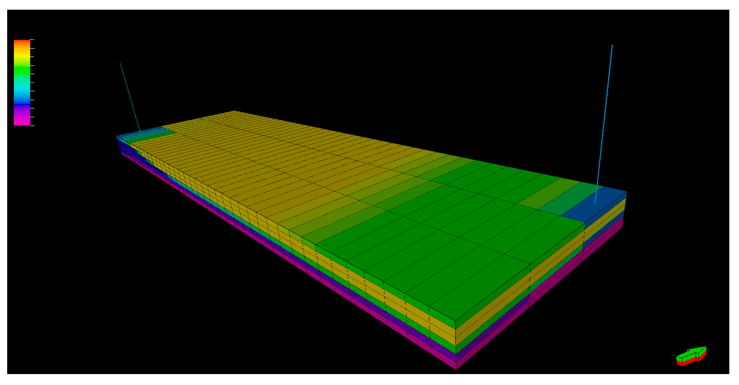
The compositional model built in Eclipse 300 was used to monitor oil, water, and gas saturation changes throughout the production cycles, specifically focusing on phase behavior and asphaltene dynamics under different operational conditions. Primary depletion resulted in pressure reduction below the bubble point, leading to gas liberation and asphaltene precipitation, which was modeled using thermodynamic and kinetic flocculation-deposition equations. The simulation was conducted using a simplified grid with a resolution of 40 × 3 × 6 to reduce computational costs while capturing overall reservoir behavior. However, this coarse grid resolution may not adequately reflect small-scale heterogeneity such as permeability, porosity, or flow paths, which are known to influence asphaltite deposition and blockage dynamics. Although the grid resolution is sufficient to demonstrate the general response trend of asphaltene to intermittent water injection strategies, it may underestimate local effects such as near-wellbore blocking or flow path deflection caused by heterogeneity. Future studies should adopt a finer grid resolution and incorporate actual geological heterogeneity to more accurately quantify deposition risks and validate model predictions.
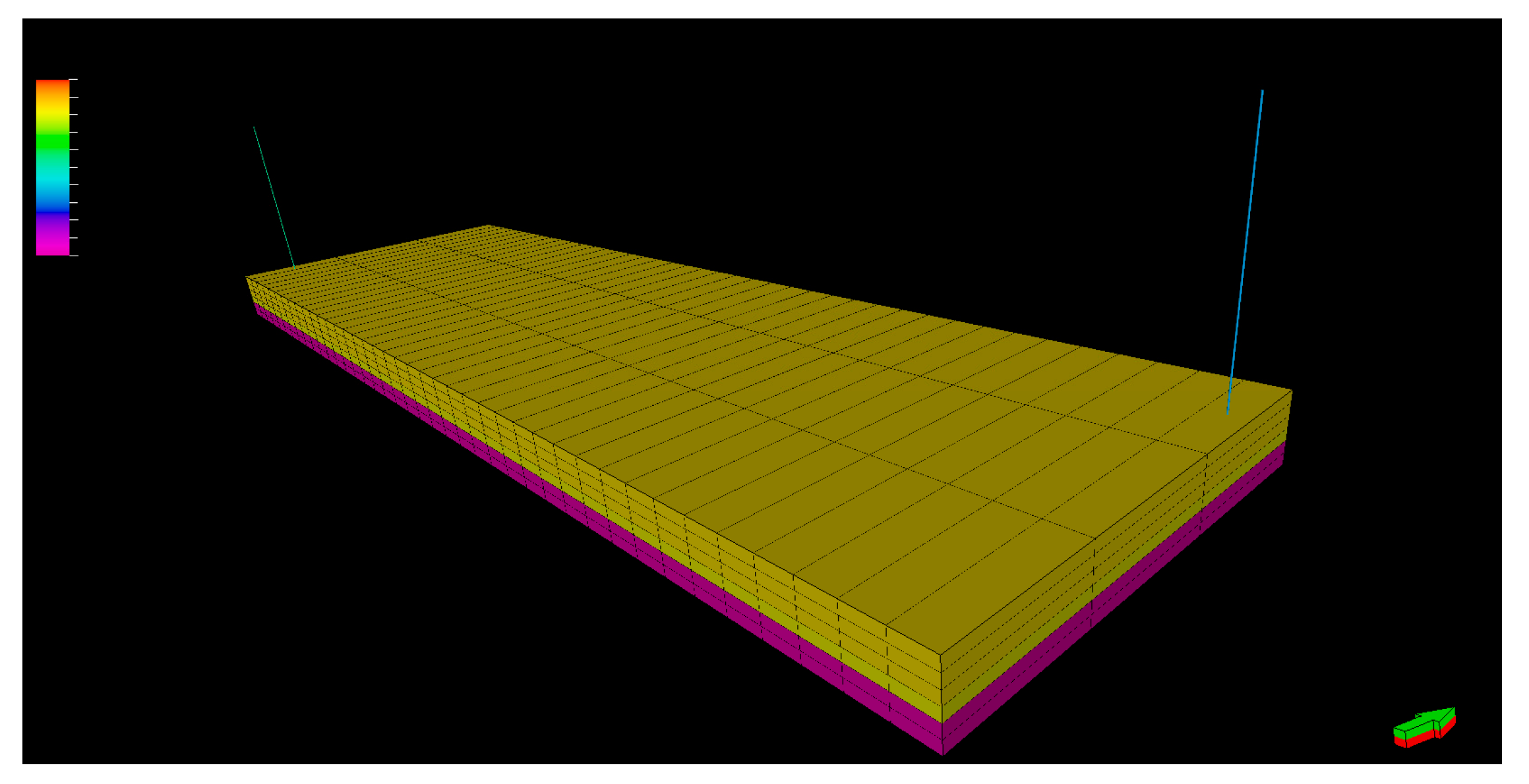
Figure 1 and Figure 2 show the initial oil saturation, with the top four layers predominantly saturated with oil and the bottom two layers with water. Gas saturation was initially zero across the domain.

Figure 1.
Oil saturation before production and injection.

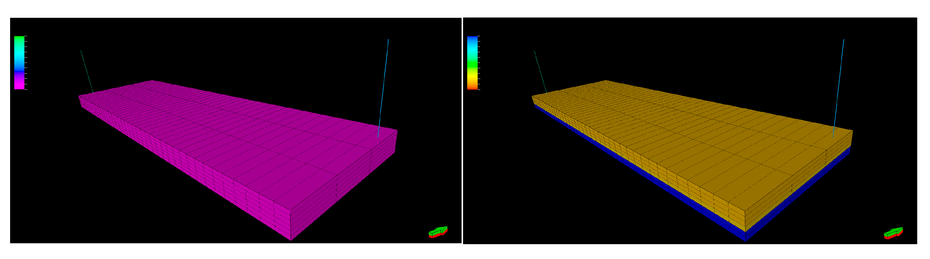
Figure 2.
Initial gas (left) and water (right) saturations. This figure shows the gas and water saturations in the reservoir before production and injection.
Following the first production cycle (primary depletion), Figure 3 and Figure 4 illustrate a drop in oil saturation and the formation of a gas cap, indicating that pressure has fallen below the bubble point. Gas emerges in the reservoir, particularly in the upper layers, while water saturation increases slightly due to fluid displacement.
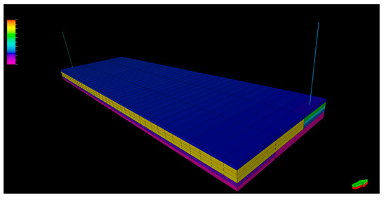
Figure 3.
Oil saturation after primary depletion. This figure shows the oil saturation following the first production interval.

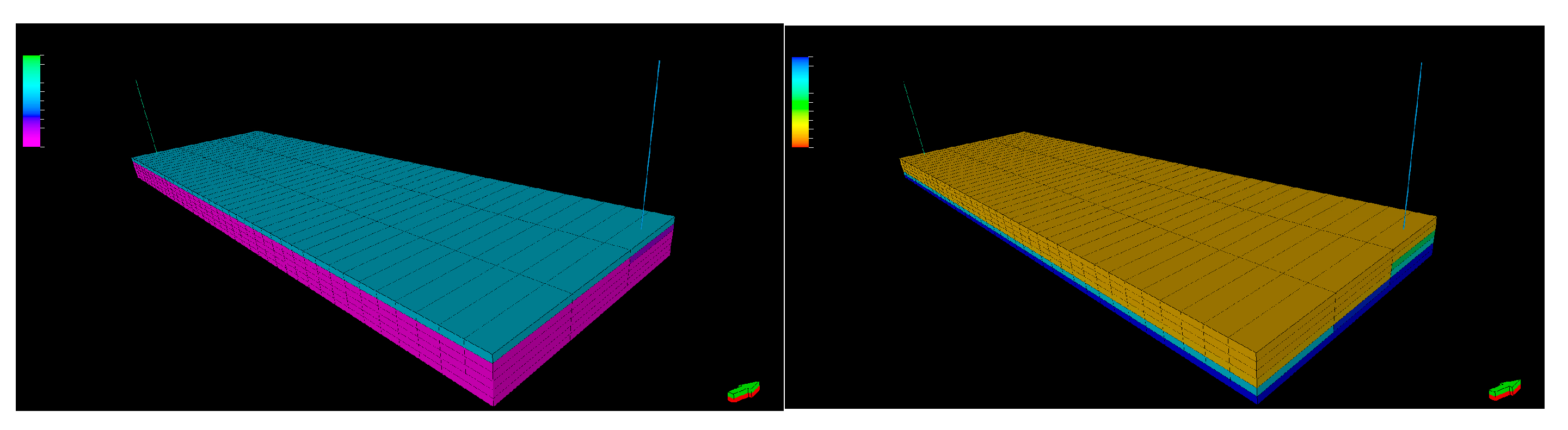
Figure 4.
Gas (left) and water (right) saturations after primary depletion. This figure shows the gas and water saturations following the first production interval.
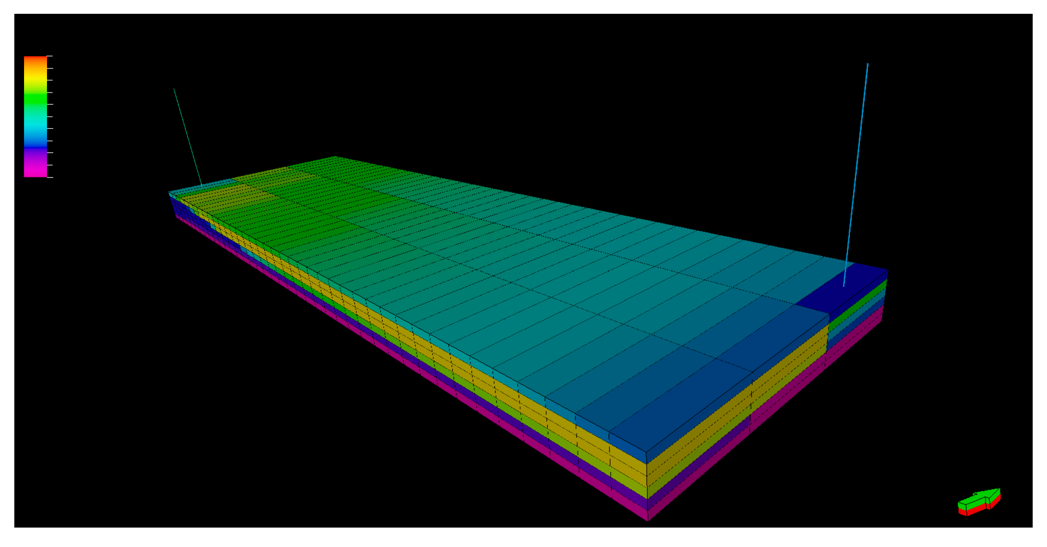
During the intermittent waterflooding phase, the injection of cooler water re-pressurizes the reservoir and changes the thermal and kinetic environment. Figure 5 and Figure 6 demonstrate how gas is partially reabsorbed into the oil phase as pressure increases above the updated bubble point. However, due to compositional changes in the oil (resulting from primary depletion), the new bubble point is different from the original, and a portion of the gas remains free.

Figure 5.
Oil saturation after injection. This figure shows the oil saturation following the intermittent waterflood interval.
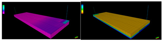
Figure 6.
Gas (left) and water (right) saturation after injection. This figure shows the gas and water saturations following the intermittent waterflood interval.
After waterflooding, the system enters a second depletion phase. Figure 7 and Figure 8 show that a second gas cap forms, but the saturation magnitude is smaller than that observed after primary depletion. This behavior confirms the shift in the phase envelope due to component redistribution and removal during production. The oil saturation continues to decline, with asphaltene deposition and permeability damage becoming more severe near the producer.
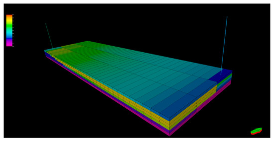
Figure 7.
Oil saturation after secondary depletion. This figure shows the oil saturation following the final production interval.
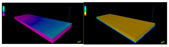
Figure 8.
Gas (left) and water (right) saturation after secondary depletion. This figure shows the gas and water saturations following the final production interval.
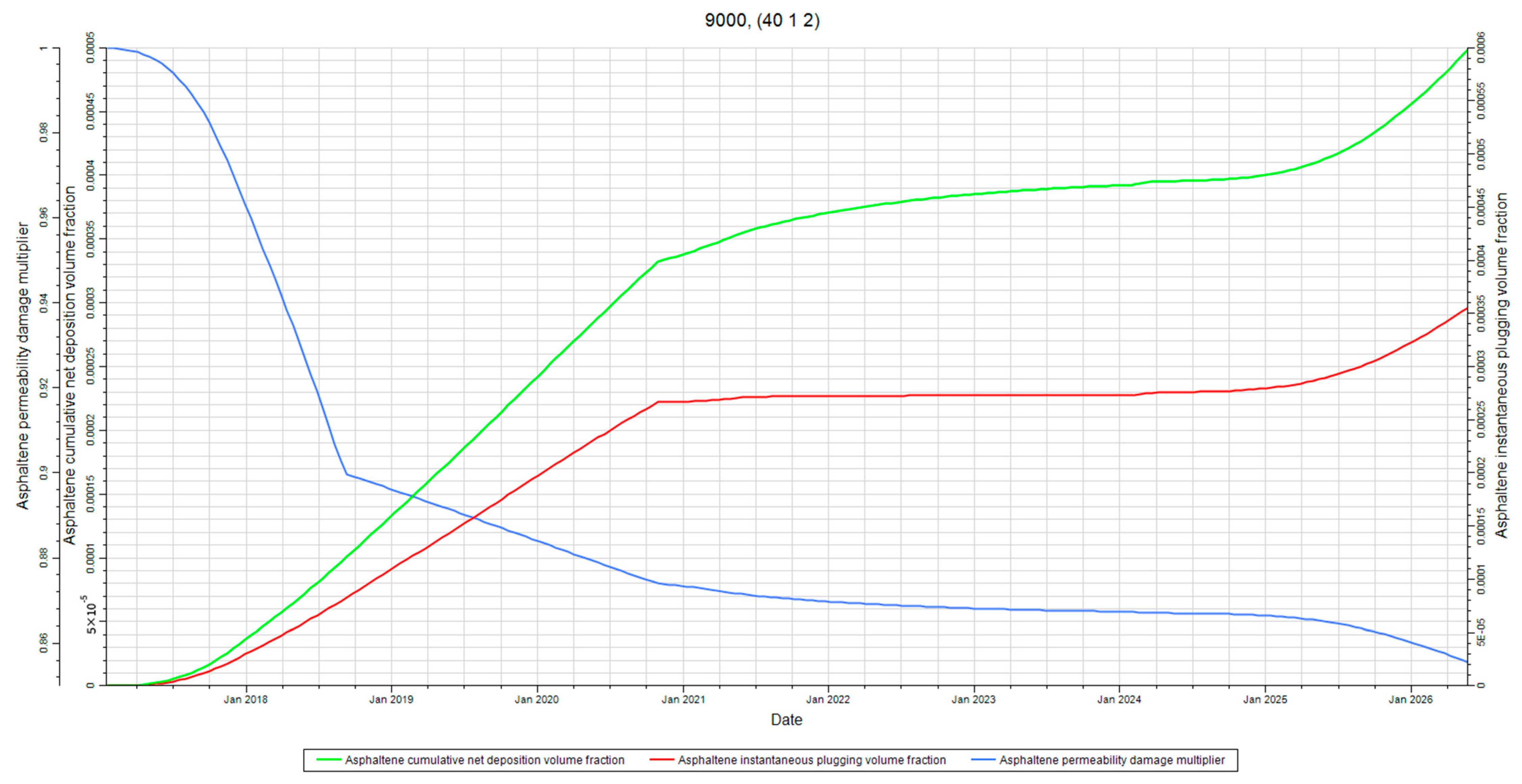
Figure 9 illustrates key reservoir parameters (pressure, gas saturation, and deposition) over time at a central grid block. The sharp drop in pressure during production corresponds to increased gas liberation and a steep rise in asphaltene deposition. The start of water injection shows a temporary spike in deposition due to cold water effects (thermal shock), followed by a stabilization trend. This re-stabilization is critical: it prevents the exponential buildup of colloidal fines and flocs that would otherwise worsen near-wellbore plugging.
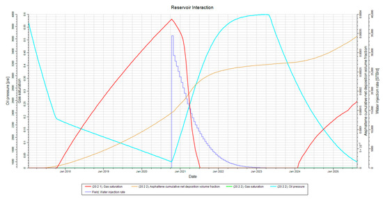
Figure 9.
Reservoir interaction. This figure illustrates various processes and behaviors in the reservoir for the entirety of the study.
3.2. Reservoir Shut-In Time Sensitivity
A sensitivity analysis was conducted to determine the influence of reservoir shut-in time on asphaltene deposition and subsequent formation damage. In this analysis, the shut-in time refers to the period between the end of the intermittent waterflooding cycle and the onset of the second production phase, during which the reservoir is completely isolated from flow.
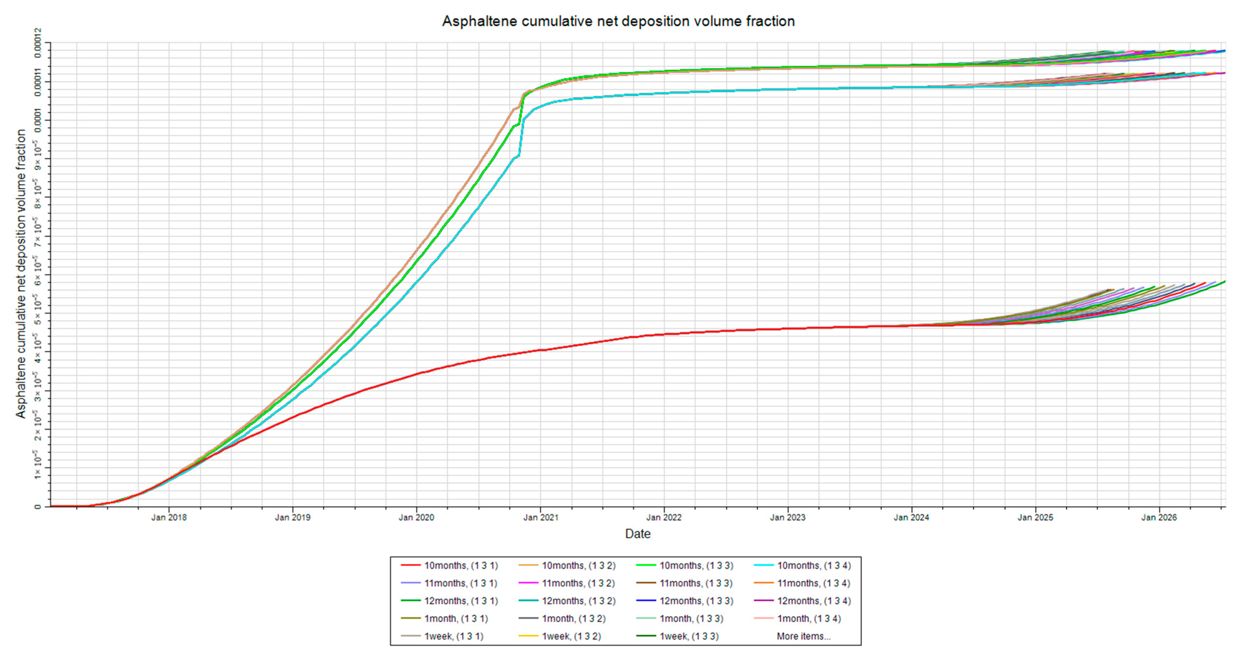
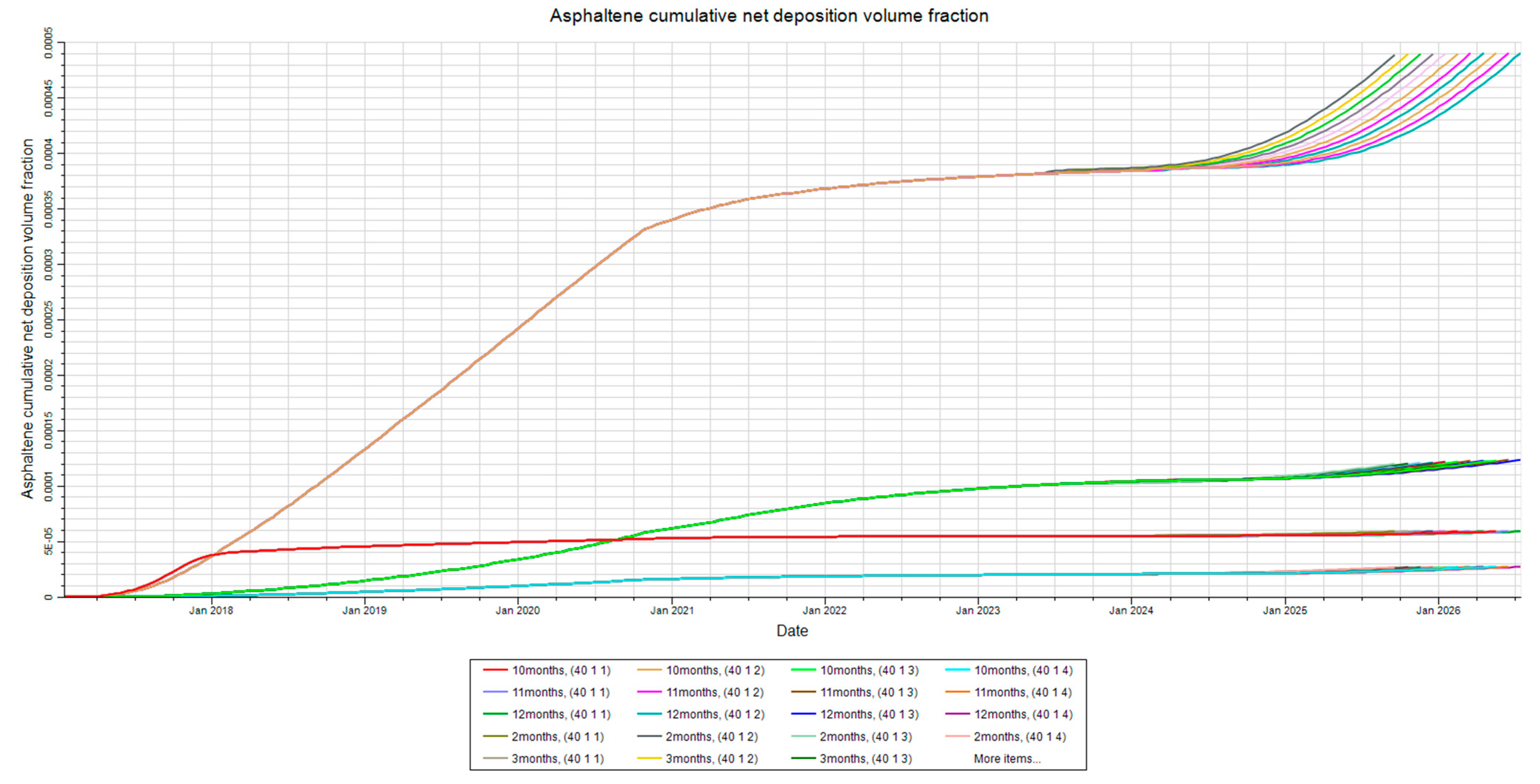
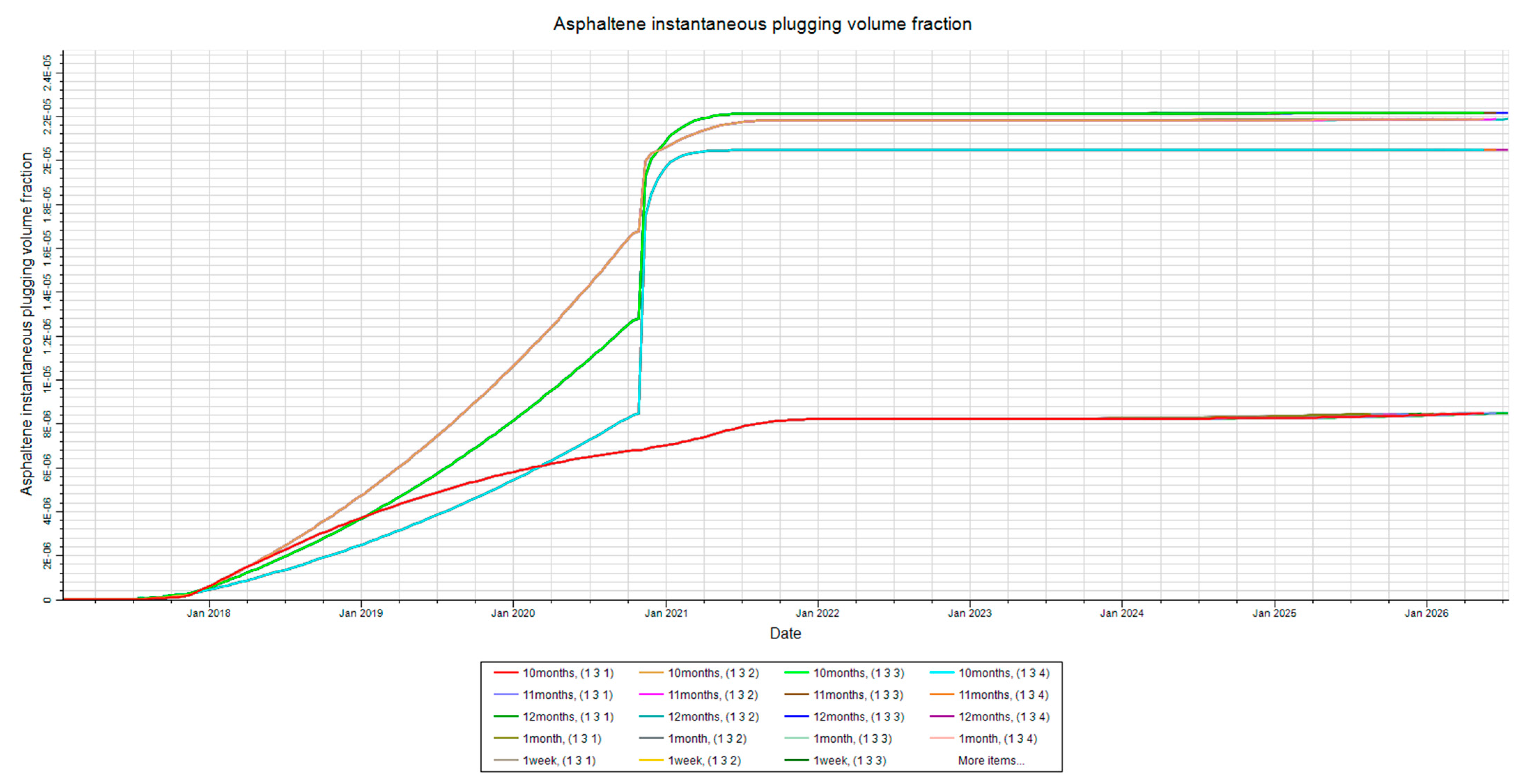
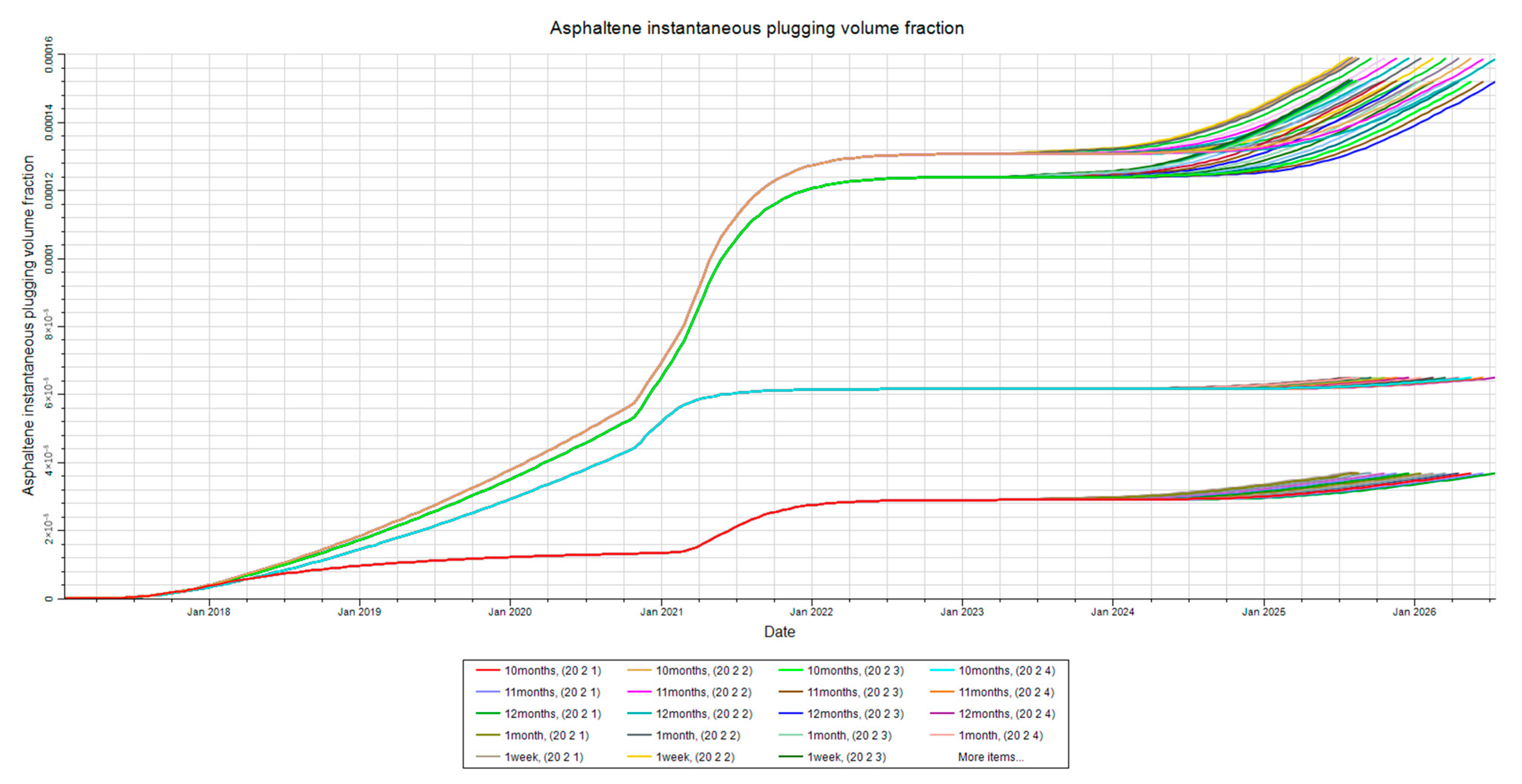
Figure 10 illustrates the varied shut-in periods tested, with the base case set at 800 days. This extended duration allows the reservoir to reach a quasi-static condition; however, simulations reveal that net deposition does not change significantly over this time frame. As shown in Figure 10, Figure 11 and Figure 12, the top asphalt deposit curves representing different well closure durations converge closely at the right end of the simulation timeline. The cumulative volume fraction values indicate minimal vertical separation, and the curves are almost parallel and overlap after 800 days. The close clustering of the upper curves indicates that the net amount of asphalt deposit tends to stabilize regardless of the well closure duration, with only minor differences in the final results. This observation suggests that prolonged shut-in may not yield additional benefits in terms of asphaltene re-dissolution and could delay oil recovery, thereby reducing economic efficiency.
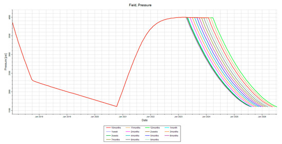
Figure 10.
Reservoir shut-in sensitivity. This figure illustrates the time shut-in time parameter that is varied for this sensitivity analysis.

Figure 11.
Deposition by injector. This figure shows the asphaltene deposition at the injector in layers 1–4 for the shut-in time sensitivity analysis.
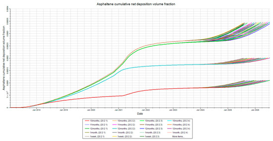
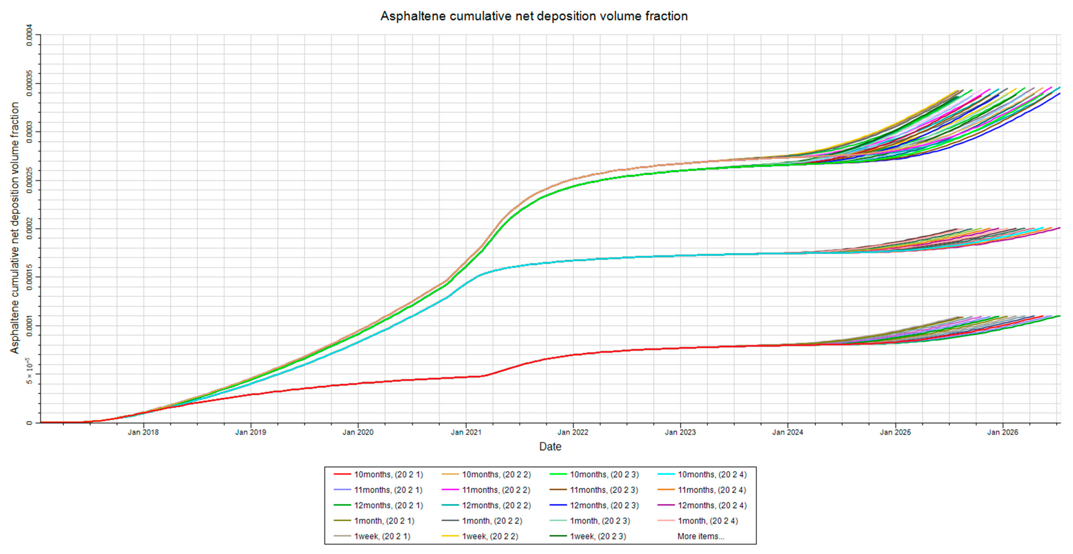
Figure 12.
Deposition at mid-point. This figure shows the asphaltene deposition at the mid-point in layers 1–4 for the shut-in time sensitivity analysis.
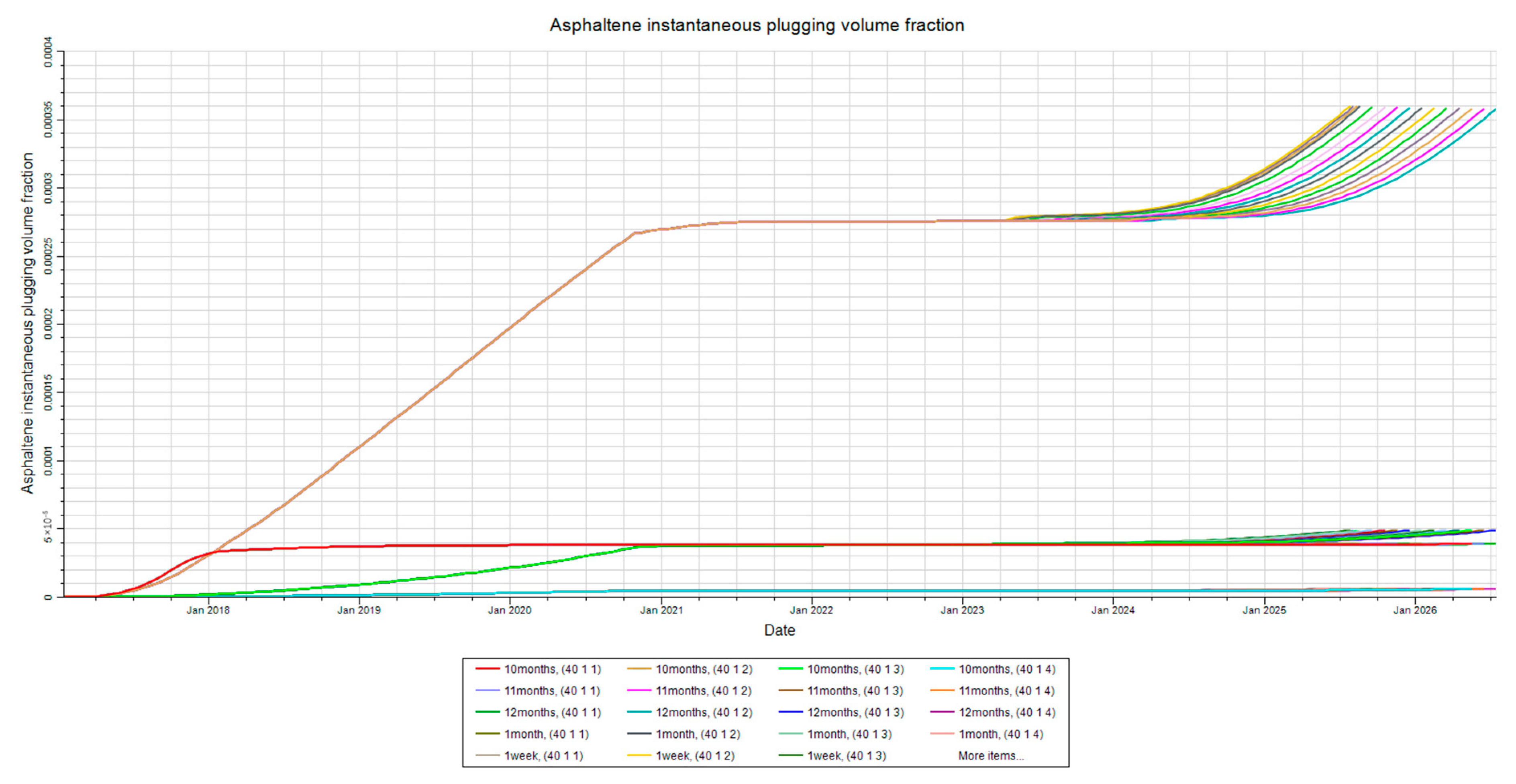
Deposition trends were analyzed at three critical locations: near the injector, at the reservoir mid-point, and near the producer. Figure 11, Figure 12 and Figure 13 display the cumulative asphaltene deposition profiles for these locations under different shut-in times. The results indicate minor fluctuations in deposition magnitudes, attributable to slight pressure drifts during the simulated shut-in, likely an artifact of the simulator’s numerical stabilization processes rather than physical flow.
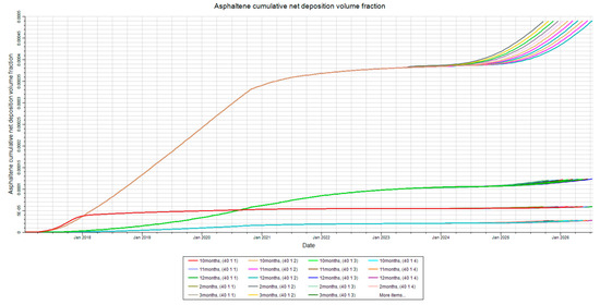
Figure 13.
Deposition at the producer. This figure shows the asphaltene deposition at the producer in layers 1–4 for the shut-in time sensitivity analysis.
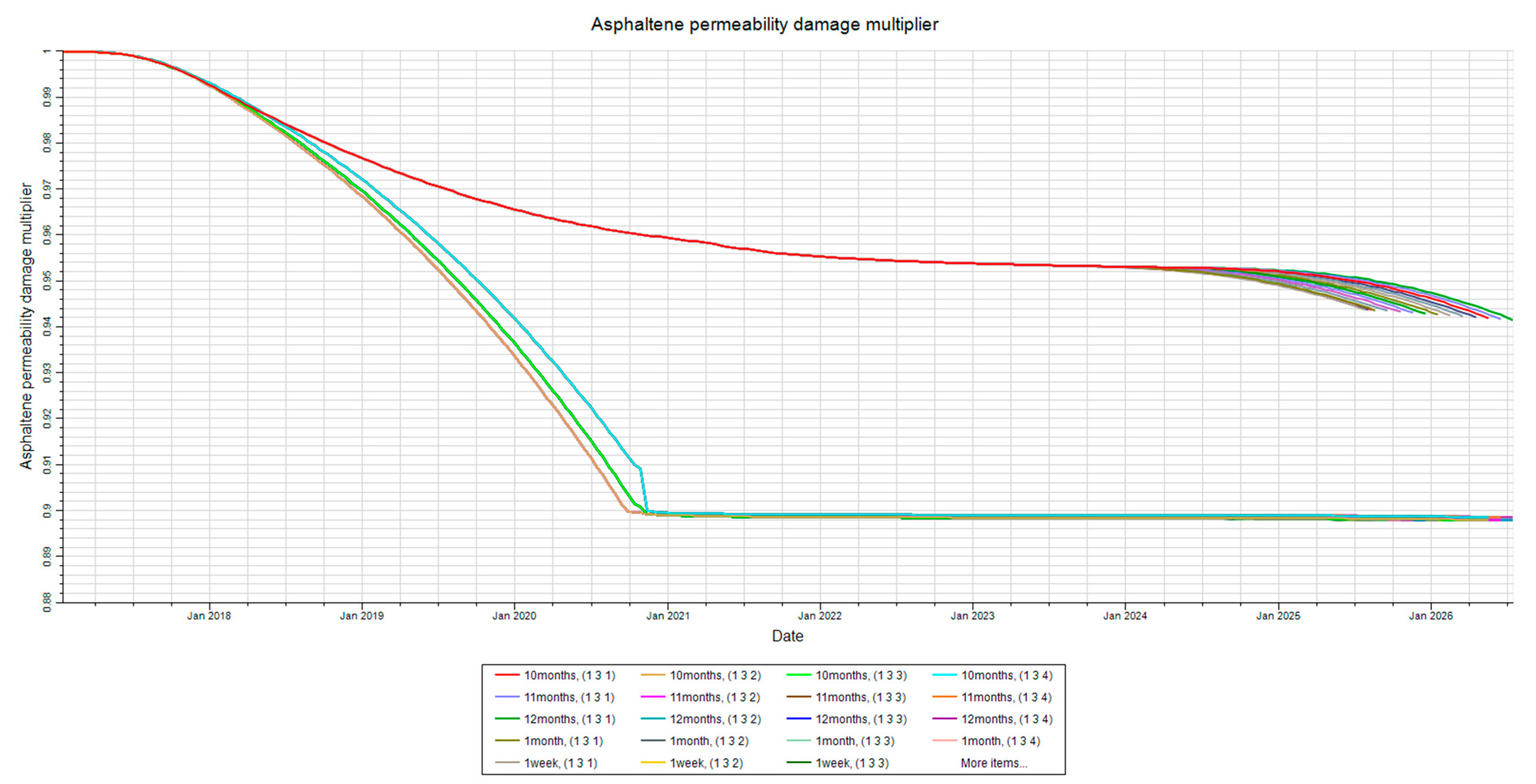
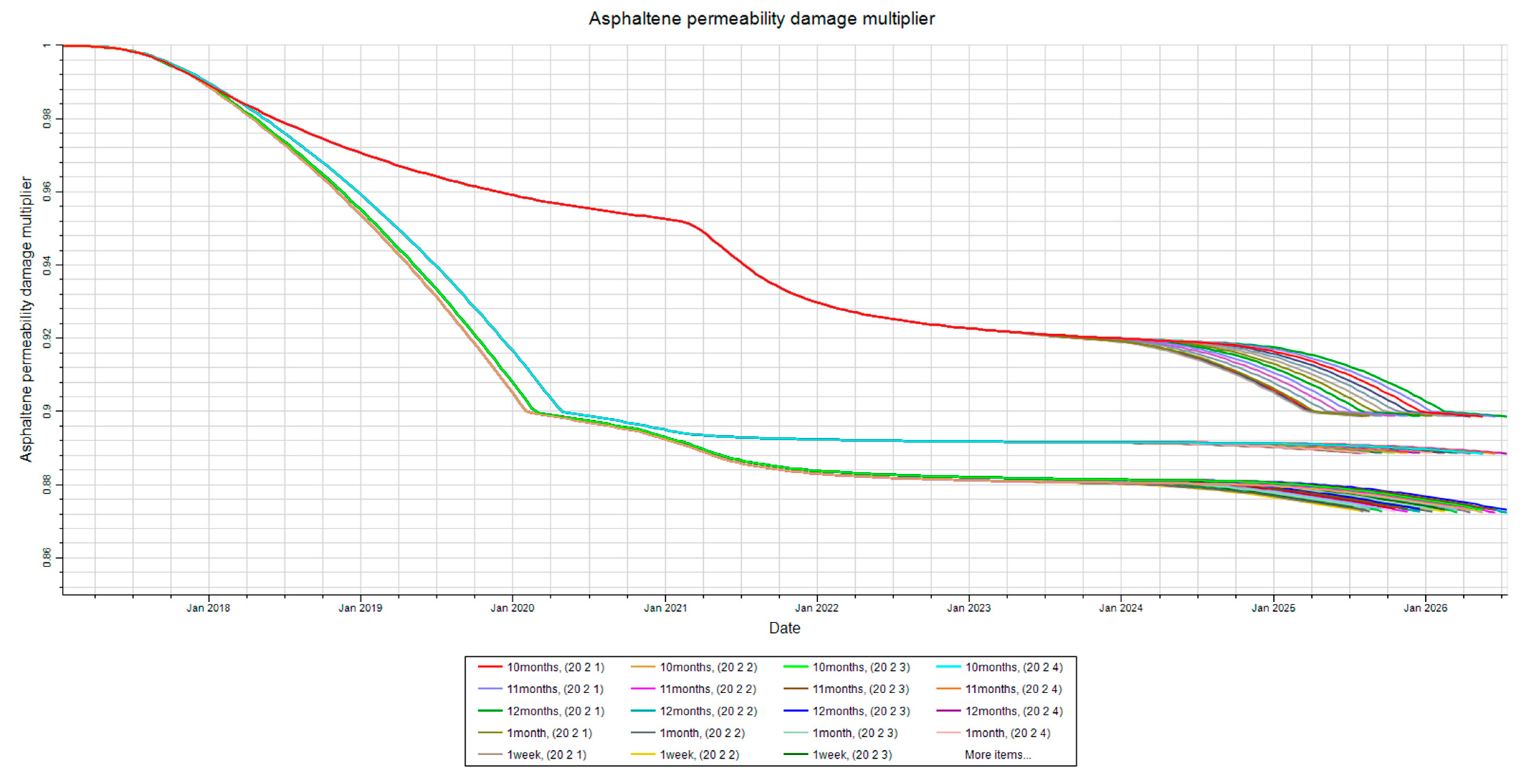
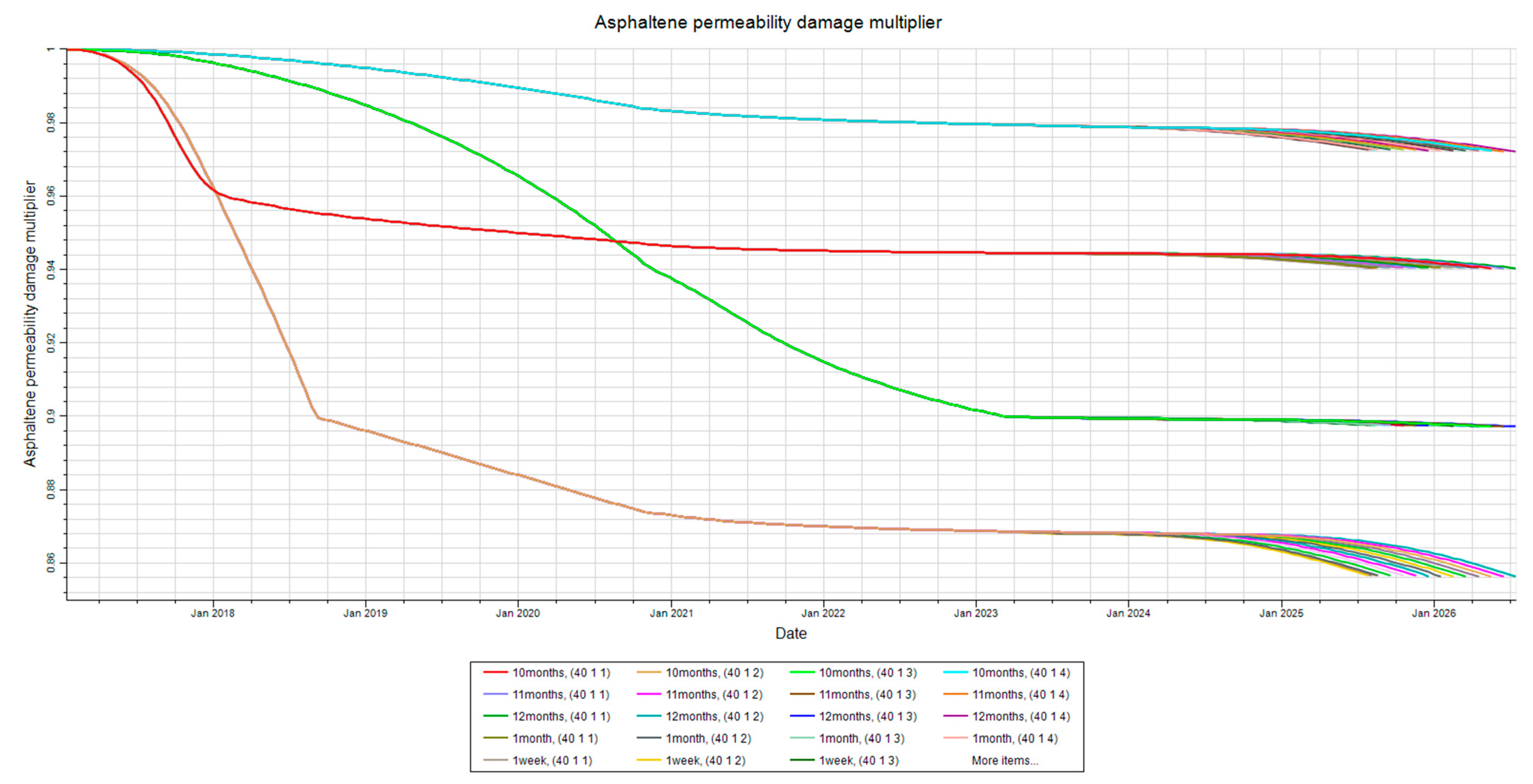
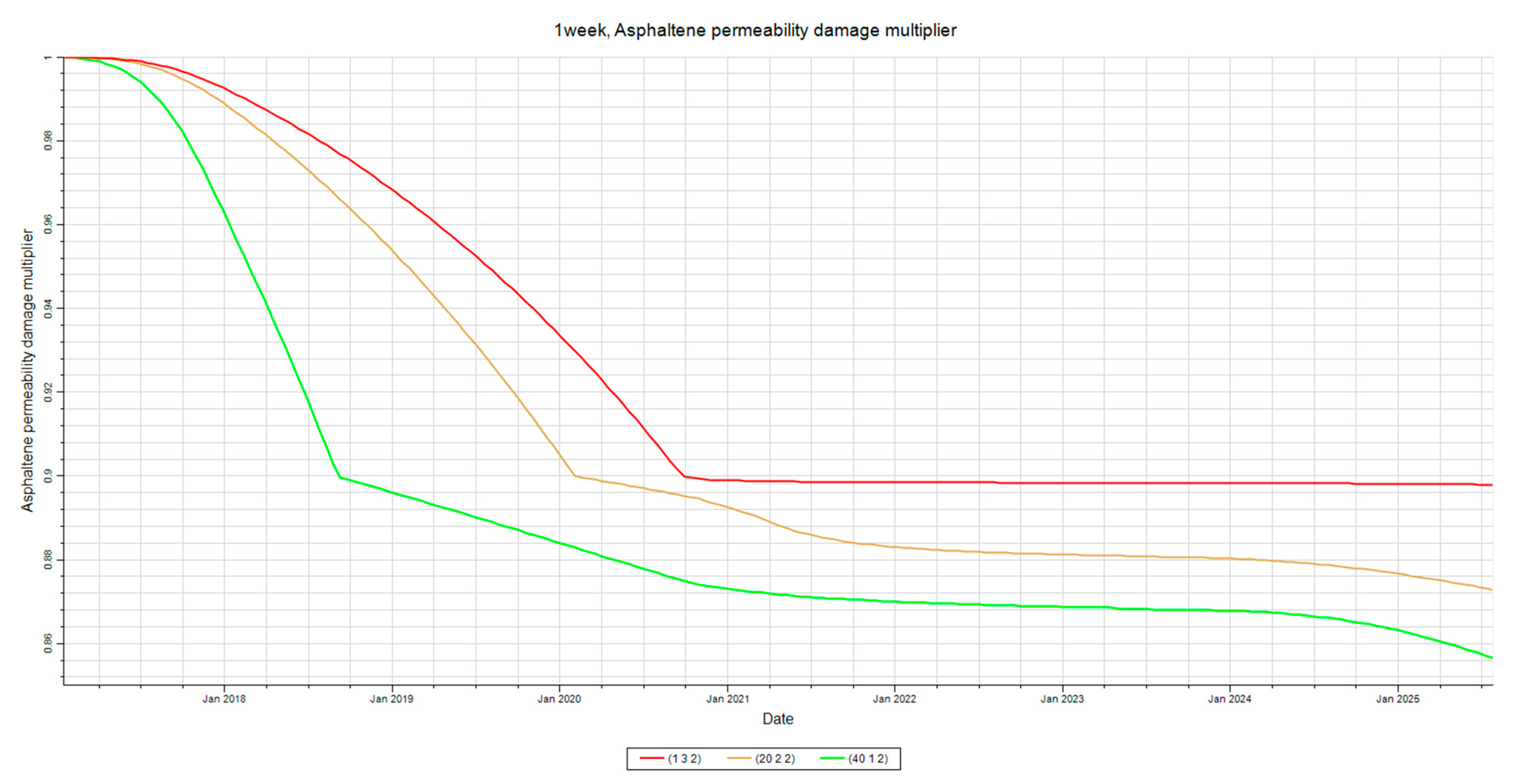
Permeability impairment resulting from asphaltene plugging follows similar patterns. Figure 14, Figure 15 and Figure 16 present the permeability damage factors at the injector, mid-point, and producer, respectively. Damage remains relatively stable across all shut-in cases, reinforcing the conclusion that extended shut-in does not significantly mitigate deposition-induced flow restrictions.
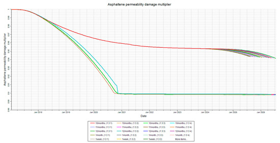
Figure 14.
Permeability damage at the injector. This figure shows the permeability damage, quantified as a multiplier, due to asphaltene deposition at the injector in layers 1–4 for the shut-in time sensitivity analysis.
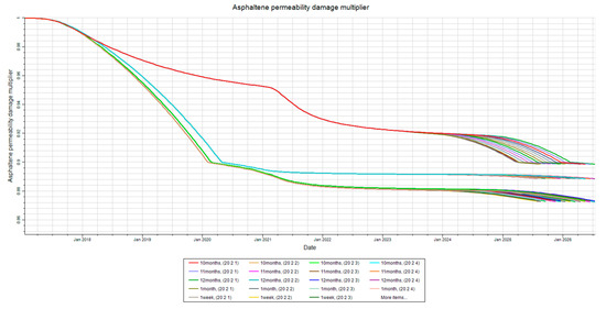
Figure 15.
Permeability damage at mid-point. This figure shows the permeability damage, quantified as a multiplier, due to asphaltene deposition at the mid-point in layers 1–4 for the shut-in time sensitivity analysis.
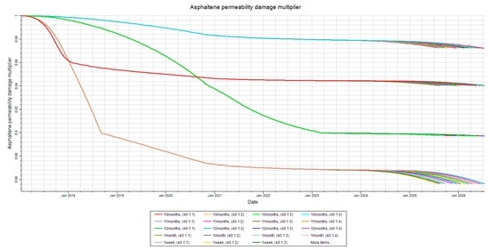
Figure 16.
Permeability damage at the producer. This figure shows the permeability damage, quantified as a multiplier, due to asphaltene deposition at the producer in layers 1–4 for the shut-in time sensitivity analysis.
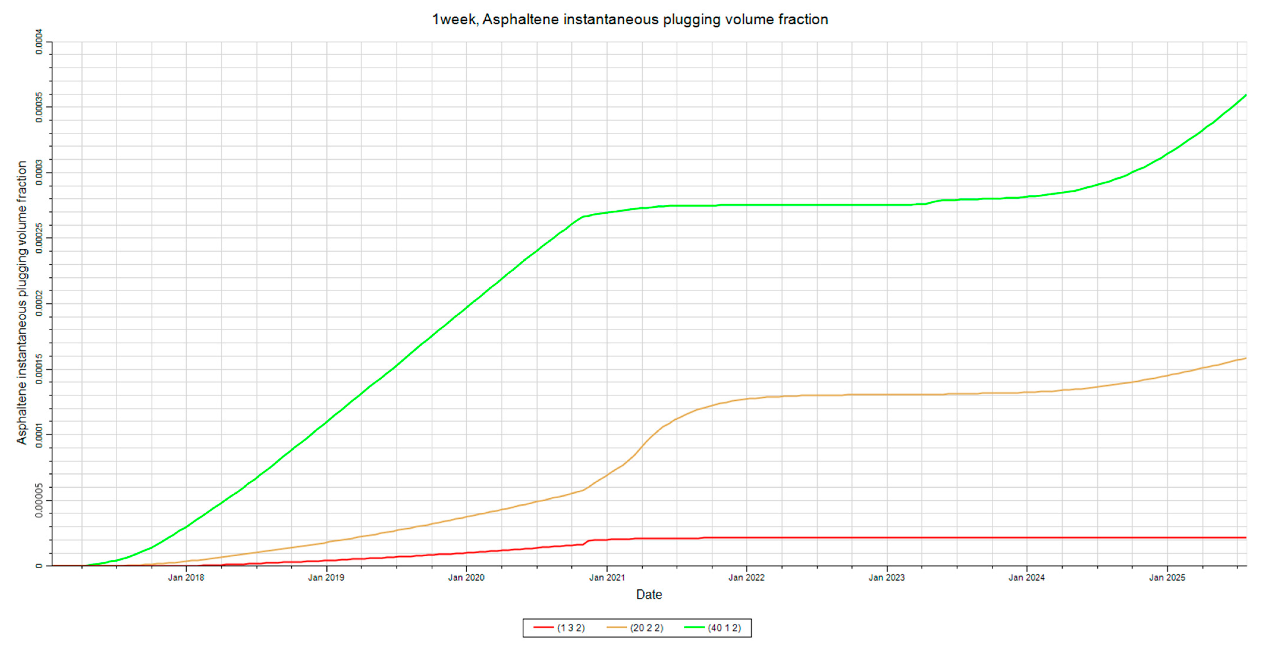
Plugging trends, shown in Figure 17, Figure 18 and Figure 19, further validate this observation. The volume fraction of asphaltene solids actively contributing to pore throat plugging remains almost constant, with negligible variations linked to numerical fluctuations rather than genuine dynamic change.

Figure 17.
Plugging at the injector. This figure shows the volume fraction of the asphaltene that is responsible for plugging pore throats in layers 1–4 for the shut-in time sensitivity analysis.
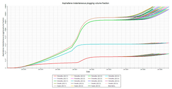
Figure 18.
Plugging at mid-point. This figure shows the volume fraction of the asphaltene that is responsible for plugging pore throats in layers 1–4 for the shut-in time sensitivity analysis.
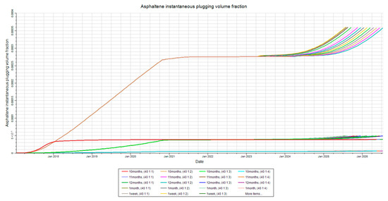
Figure 19.
Plugging at the producer. This figure shows the volume fraction of the asphaltene that is responsible for plugging pore throats in layers 1–4 for the shut-in time sensitivity analysis.
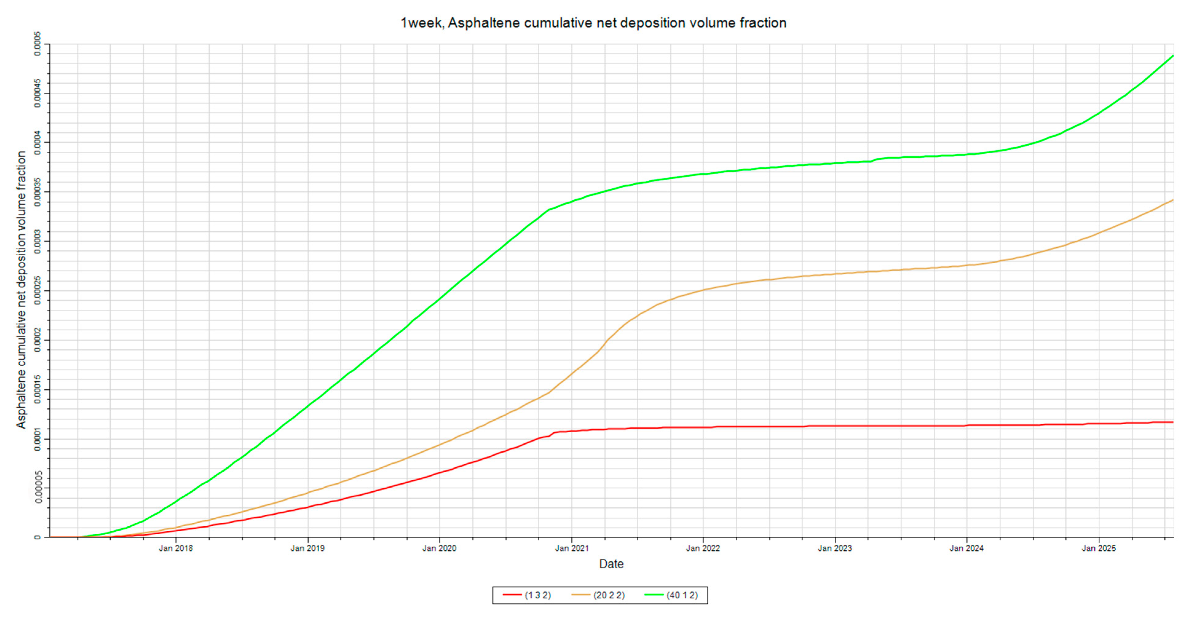
Finally, Figure 20, Figure 21 and Figure 22 consolidate deposition, permeability damage, and plugging effects by location for a representative layer, demonstrating that the near-producer region consistently experiences the highest damage due to increased drawdown and streamline convergence.
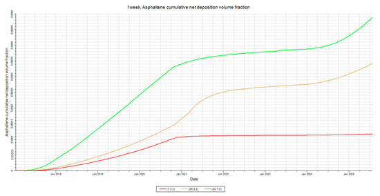
Figure 20.
Deposition at the producer, mid-point. This figure shows the asphaltene deposition in layer two at all three locations of inspection for the shut-in time sensitivity analysis.
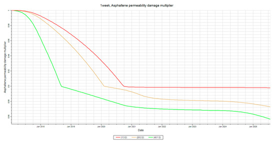
Figure 21.
Permeability damage at the injector, mid-point, and the producer. This figure shows the permeability damage in layer two at all three locations of inspection for the shut-in time sensitivity analysis.
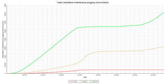
Figure 22.
Plugging at the injector, mid-point, and the producer. This figure shows the asphaltene volume responsible for plugging pore throats in layer two at all three locations of inspection for the shut-in time sensitivity analysis.
These findings emphasize that while intermittent waterflooding inherently helps manage asphaltene deposition by introducing cyclic re-stabilization, the shut-in duration must be carefully optimized to balance reservoir re-equilibration with economic oil recovery targets. Based on these results, production should ideally resume within the first week after waterflooding to maintain operational feasibility and minimize deferred production.
3.3. Spatial Deposition Trends Under Shut-In Sensitivity
Spatial analysis of asphaltene behavior reveals that deposition effects are most severe in the near-producer region, consistent with expectations regarding pressure drawdown and streamline convergence. Figure 20, Figure 21 and Figure 22 previously established that deposition, permeability impairment, and plugging were highest at the producer. This section provides additional insights into the spatial behavior of asphaltenes during shut-in sensitivity runs, focusing on how flow dynamics influence the distribution of deposition-related damage.
Figure 13, Figure 14 and Figure 15 illustrate that asphaltene effects—namely deposition, plugging, and permeability damage—diminish with increasing distance from the producer. These results follow physical expectations and align with previous studies. The fundamental mechanism involves pressure drawdown and kinetic energy gradients. As fluid flows toward the producer, suspended asphaltene flocs experience drag and aggregation, resulting in concentrated flocculation near the wellbore. The destabilized oil phase in this region is more prone to precipitate asphaltenes, which subsequently aggregate and deposit.
Furthermore, the accumulation of flow streamlines near the production well intensifies this phenomenon. As shown in Figure 23, streamline convergence amplifies local floc concentrations and kinetic energy changes, further promoting deposition. The destabilization of the oil phase in this zone increases the probability of irreversible floc formation and pore-scale damage.
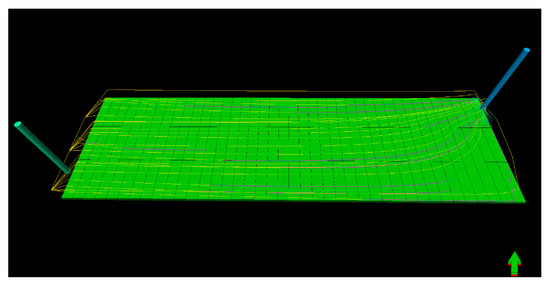
Figure 23.
Streamlines during production. This figure illustrates the streamlines at a point in time during production in order to highlight the convergence at the producer.
The combined effect of fluid drag, drawdown-induced destabilization, and streamline convergence results in a higher exposure of pore throats to asphaltene flocs, increasing the risk of plugging and permeability loss. These dynamics explain the consistent observation of maximum damage near the producer, even under varying shut-in durations. The mid-point and injector regions experience lower drawdown and weaker convergence, which explains their relatively lower asphaltene-related damage.
These spatial trends validate the importance of tailoring operational strategies—especially production restart timing and flowrate ramp-up—to limit damage in critical zones. Maintaining system stability near the producer is crucial for sustaining injectivity and overall recovery efficiency in reservoirs susceptible to asphaltene-related flow impairment.
3.4. Injection Rate Sensitivity
Injection rate plays a critical role in asphaltene deposition, as it governs thermal, compositional, and flow-induced changes in the reservoir. This section evaluates the sensitivity of deposition and plugging behavior to different water injection rates under fixed pressure constraints.
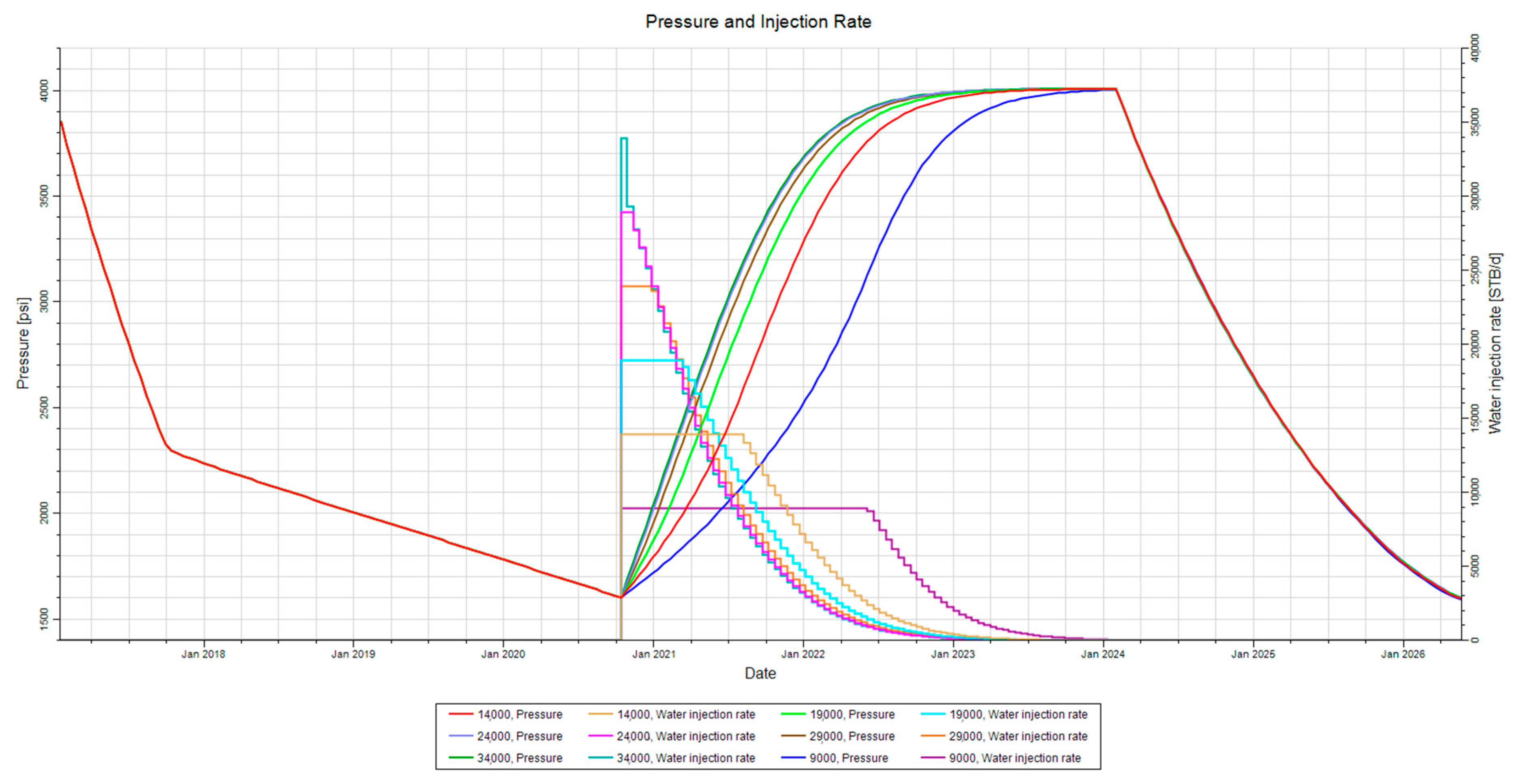
Figure 24 shows the five injection rates examined, ranging from 9000 to 34,000 stb/day, with a 5000 stb/day increment (ΔQi = 5000 stb/day). Each case was capped at a maximum bottomhole pressure (BHP) of 4000 psi, selected to remain below the estimated fracture pressure of the formation. This BHP ceiling terminates injection once the pressure limit is reached, ensuring physical realism.

Figure 24.
Injection rate variance. This figure illustrates how the injection rate is varied for this sensitivity analysis.
3.4.1. Deposition Trends at Key Locations
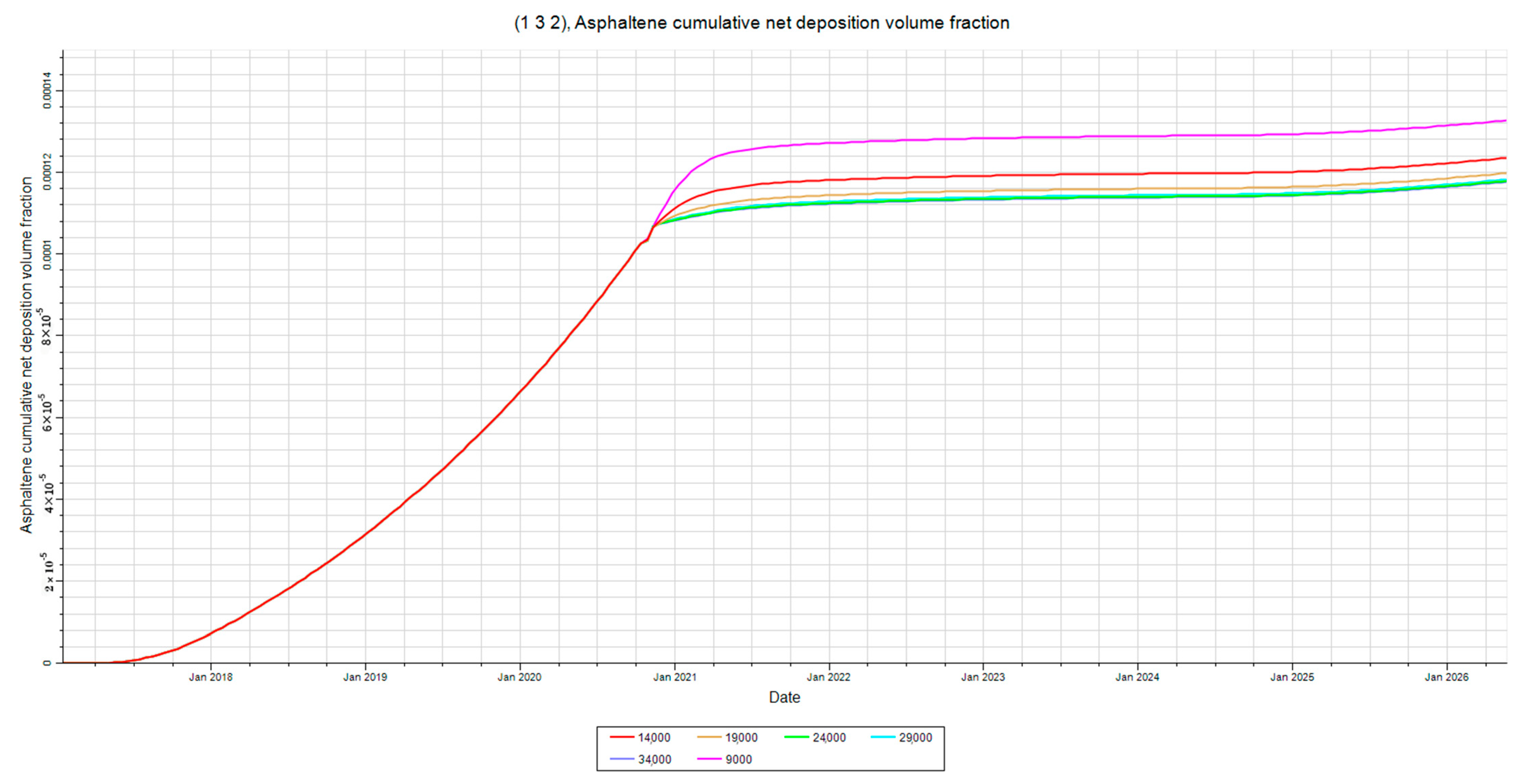
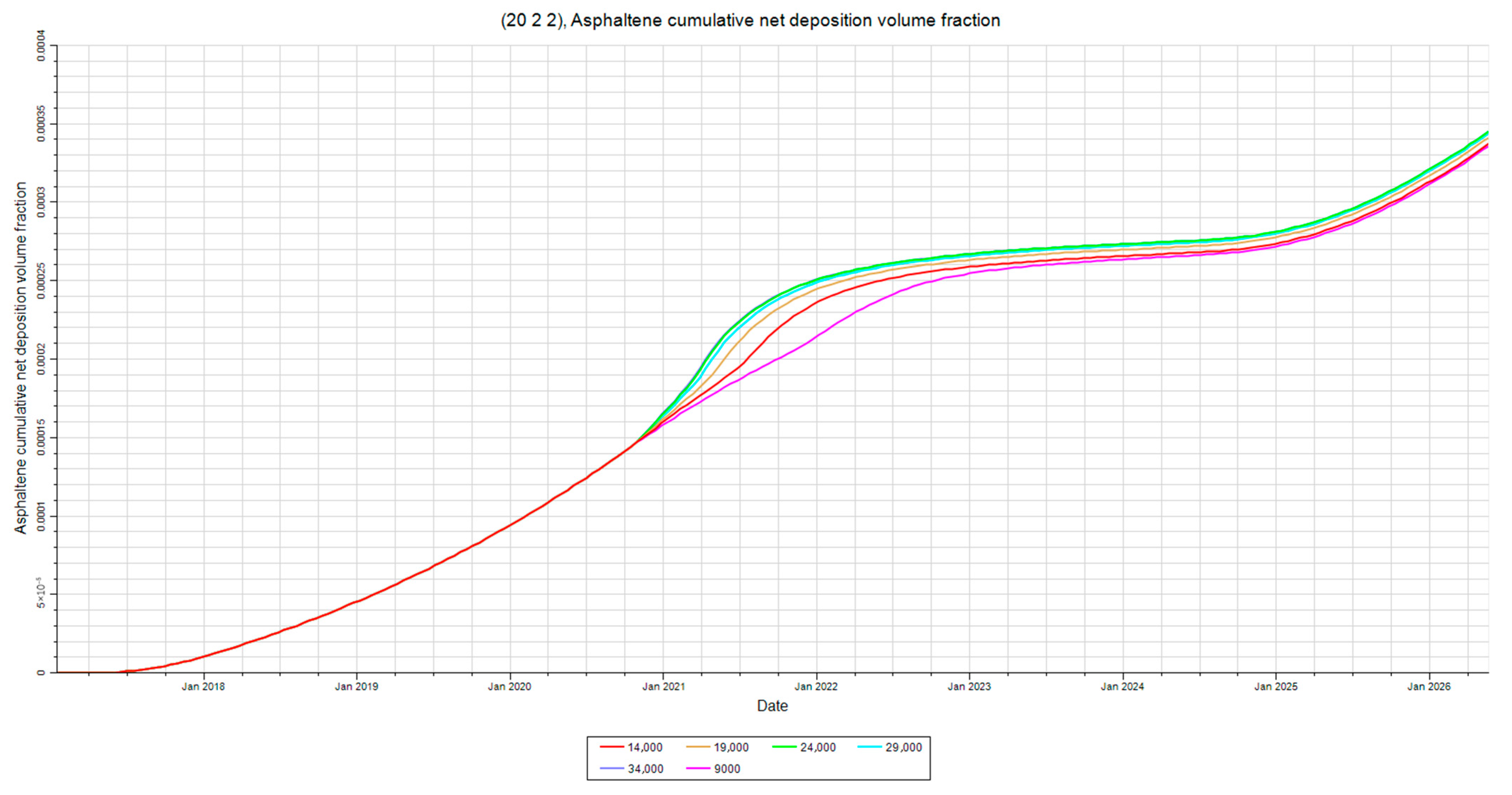
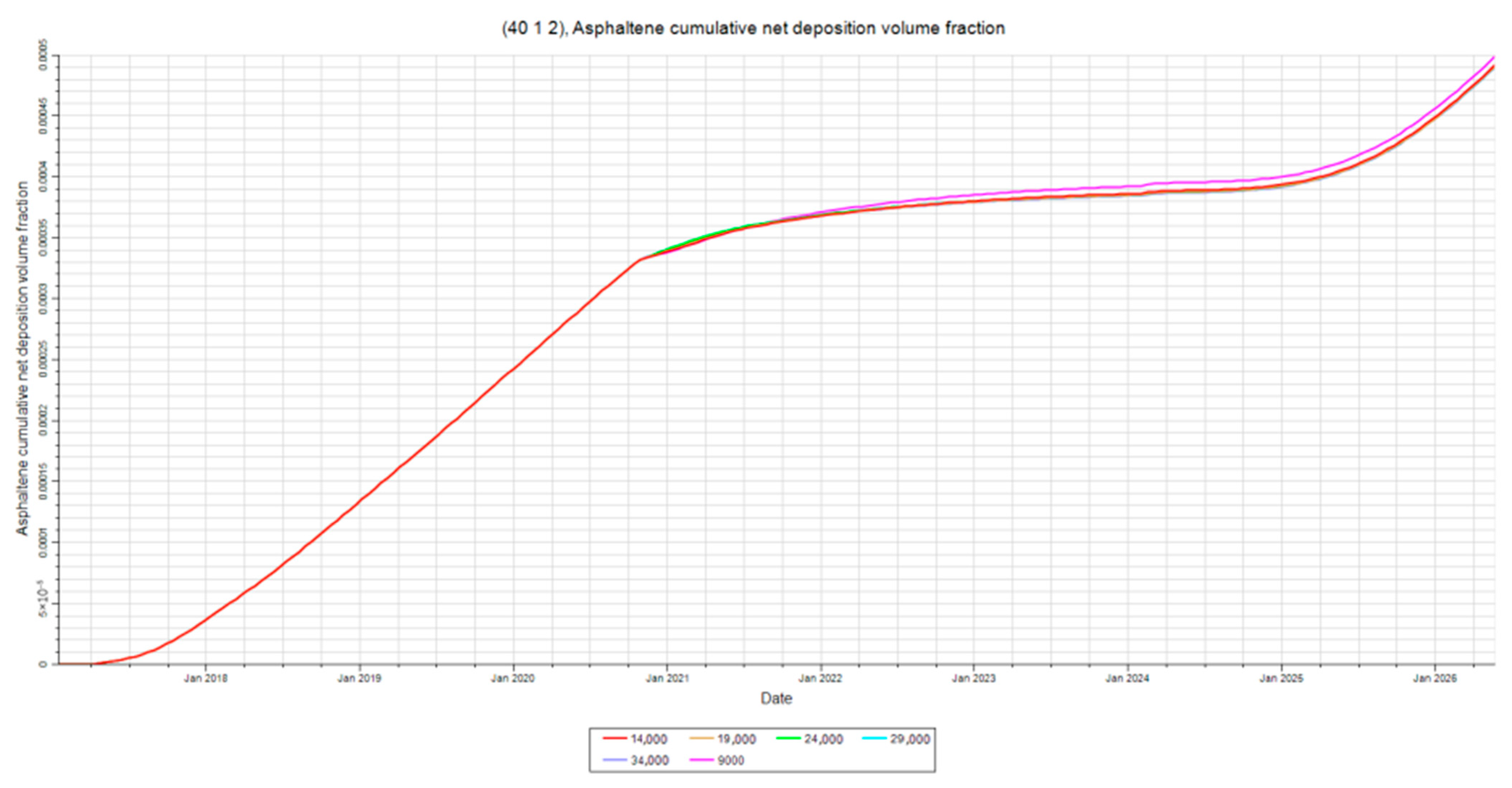
Figure 25, Figure 26 and Figure 27 illustrate asphaltene deposition responses at the injector, reservoir midpoint, and producer for each injection rate tested.
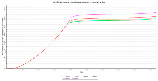
Figure 25.
Deposition at the injector. This figure shows the asphaltene deposition at the injector in layer 2 for the injection rate sensitivity analysis.
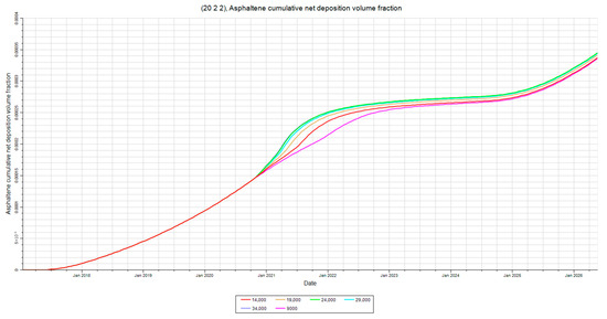
Figure 26.
Deposition at mid-point. This figure shows the asphaltene deposition at the mid-point in layer 2 for the injection rate sensitivity analysis.
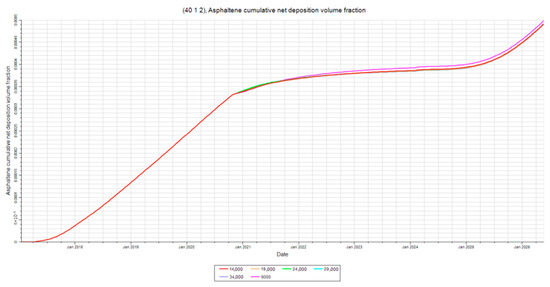
Figure 27.
Deposition at the producer. This figure shows the asphaltene deposition at the producer in layer 2 for the injection rate sensitivity analysis.
At injection rates above 19,000 stb/day, deposition trends plateau, suggesting a limit to flow-induced destabilization. However, lower injection rates result in markedly higher deposition near the injector and producer. This is attributed to longer injection durations under these low-flow conditions, which increase thermal disequilibrium between the cold water and the formation, enhancing flocculation near wellbores.
Interestingly, deposition decreases at the mid-point under lower flow rates. This trend is likely driven by heavy component accumulation in the central reservoir zone, which stabilizes asphaltenes locally. Conversely, higher injection rates accelerate floc transport toward the mid-point, increasing deposition there.
Table 3 the summarizes estimated asphaltene deposition at the injector, mid-point, and producer locations for various injection rates, based on the trends observed in Figure 25, Figure 26 and Figure 27. It also includes an approximation of the maximum permeability reduction associated with each scenario. These values provide a comparative view of how injection rate influences deposition distribution and reservoir damage, supporting the conclusion that higher injection rates mitigate producer-end plugging and improve reservoir flow conditions.
Table 3.
Effect of injection rate on asphaltene deposition and permeability reduction.
In the simulation, the role of flocculate entrainment in asphalt transport was accounted for through the “entrain” parameter in the ASPDEPO keywords. Although deposition and blocking effects were more pronounced in the results, entrainment plays a subtle yet important role in redistributing flocculates under dynamic flow conditions. Especially during the water injection phase, entrained flocculates may be transported to areas beyond the injection point and subsequently re-deposit in low-flow velocity zones or accumulate in the medium-oil layer. This mechanism explains the spatial variation in deposition patterns, particularly the increase in midpoint deposition at high water injection rates. Although entrained mass was not explicitly tracked in the output summary, its contribution is implicitly captured through changes in local deposition profiles. Future studies will conduct a dedicated sensitivity analysis of the entrained mass coefficient to more clearly isolate and quantify this effect.
3.4.2. Plugging and Permeability Impairment
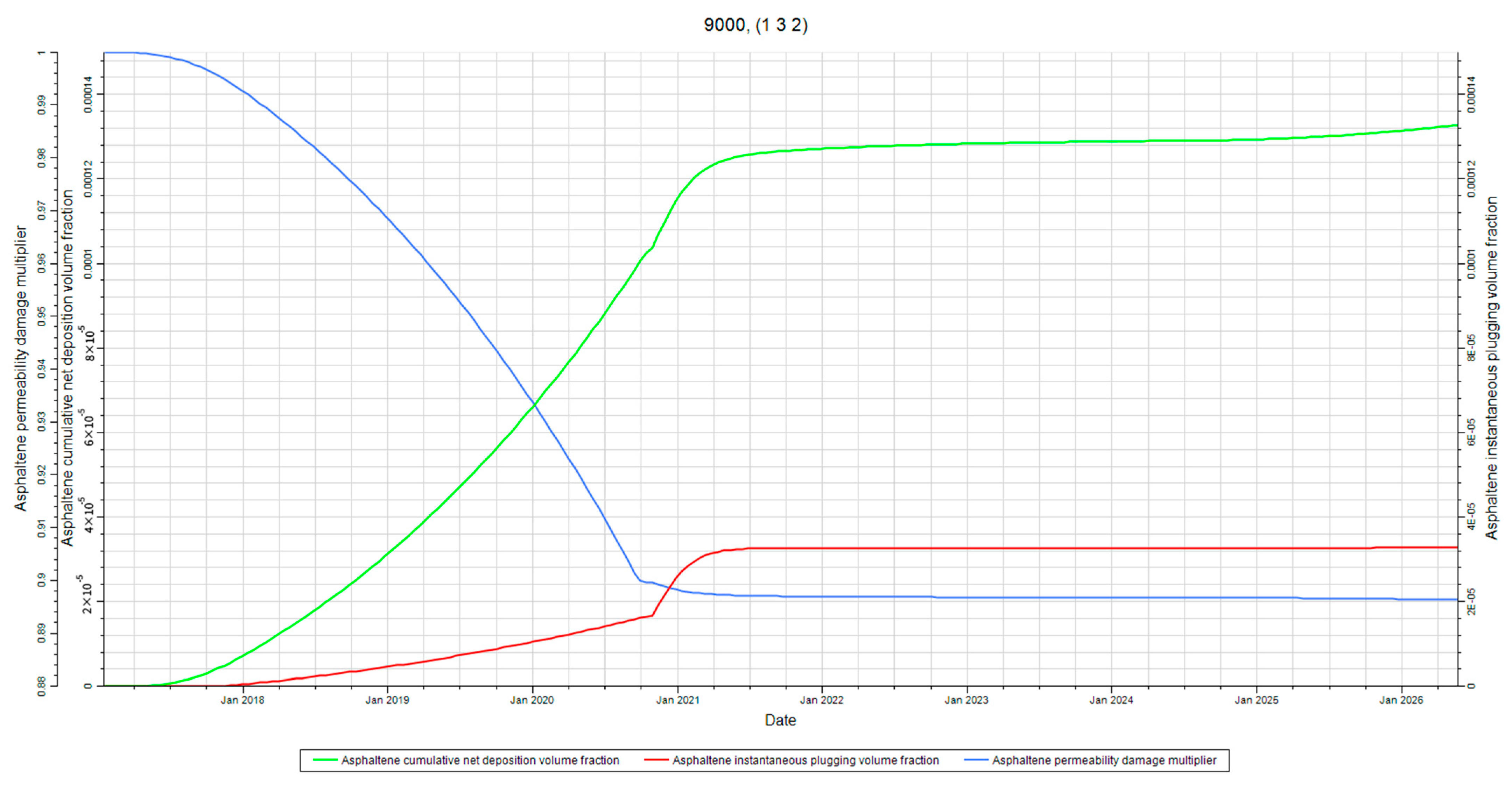
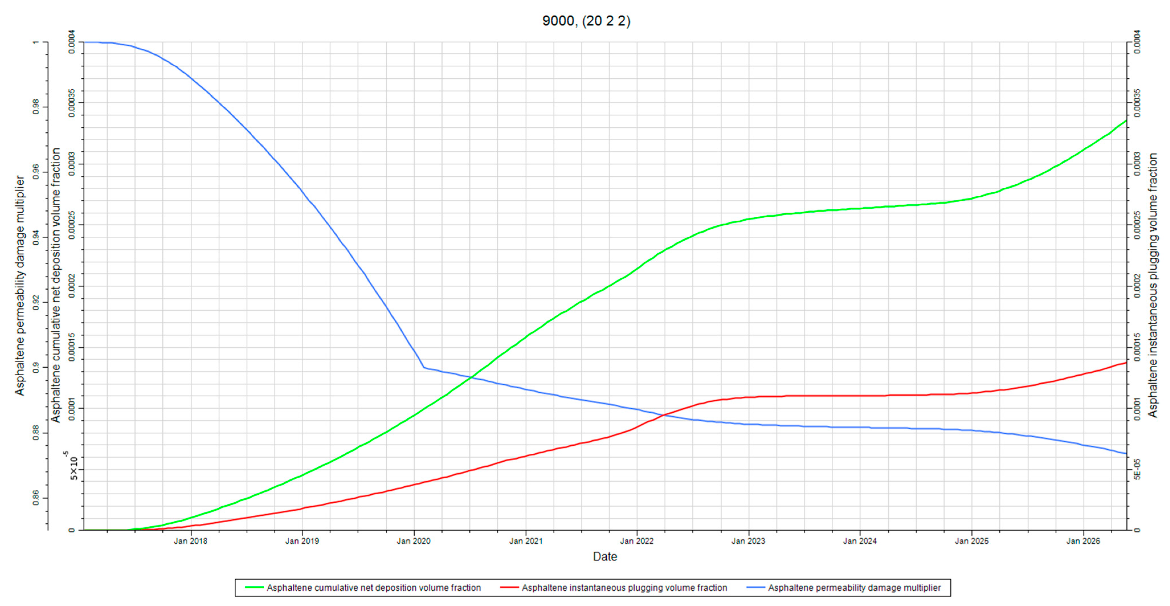
Figure 28, Figure 29 and Figure 30 consolidate the deposition, permeability damage, and plugging factors at the same three locations. These figures show that plugging and permeability loss track closely with deposition trends, reaffirming the link between floc concentration and pore-scale damage.
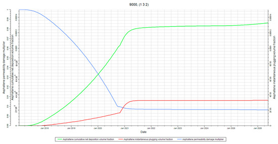
Figure 28.
Deposition, permeability, and plugging at the injector. This figure shows all three outputs evaluated for this study at the injector in layer 2.

Figure 29.
Deposition, permeability, and plugging at mid-point. This figure shows all three outputs evaluated for this study at the mid-point in layer 2.
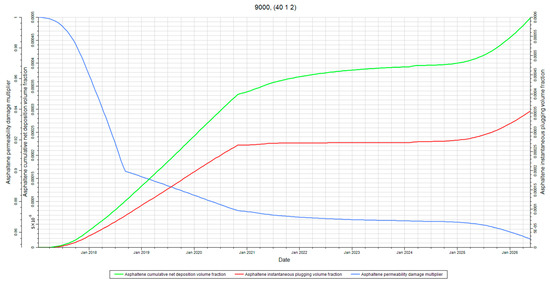
Figure 30.
Deposition, permeability, and plugging at the producer. This figure shows all three outputs evaluated for this study at the producer in layer 2.
A notable pattern emerges: plugging effects converge spatially toward the producer, regardless of injection rate. This is consistent with the physical mechanisms discussed in Section 3.2—specifically streamline convergence and drawdown-enhanced destabilization. The pressure gradient near the producer intensifies floc movement and aggregation, exposing more pore throats to plugging.
3.4.3. Operational Implications
These results suggest that higher injection rates are favorable in mitigating near-producer deposition and enhancing economic feasibility. Faster injection reduces contact time between the cold water and crude oil, minimizing temperature-induced destabilization and decreasing the duration of low-mobility conditions.
In field applications, this finding supports the use of aggressive injection during cycling, provided formation integrity is preserved. Minimizing deposition at the producer protects long-term productivity and delays the onset of severe plugging or permeability impairment.
3.5. Time of Injection Sensitivity
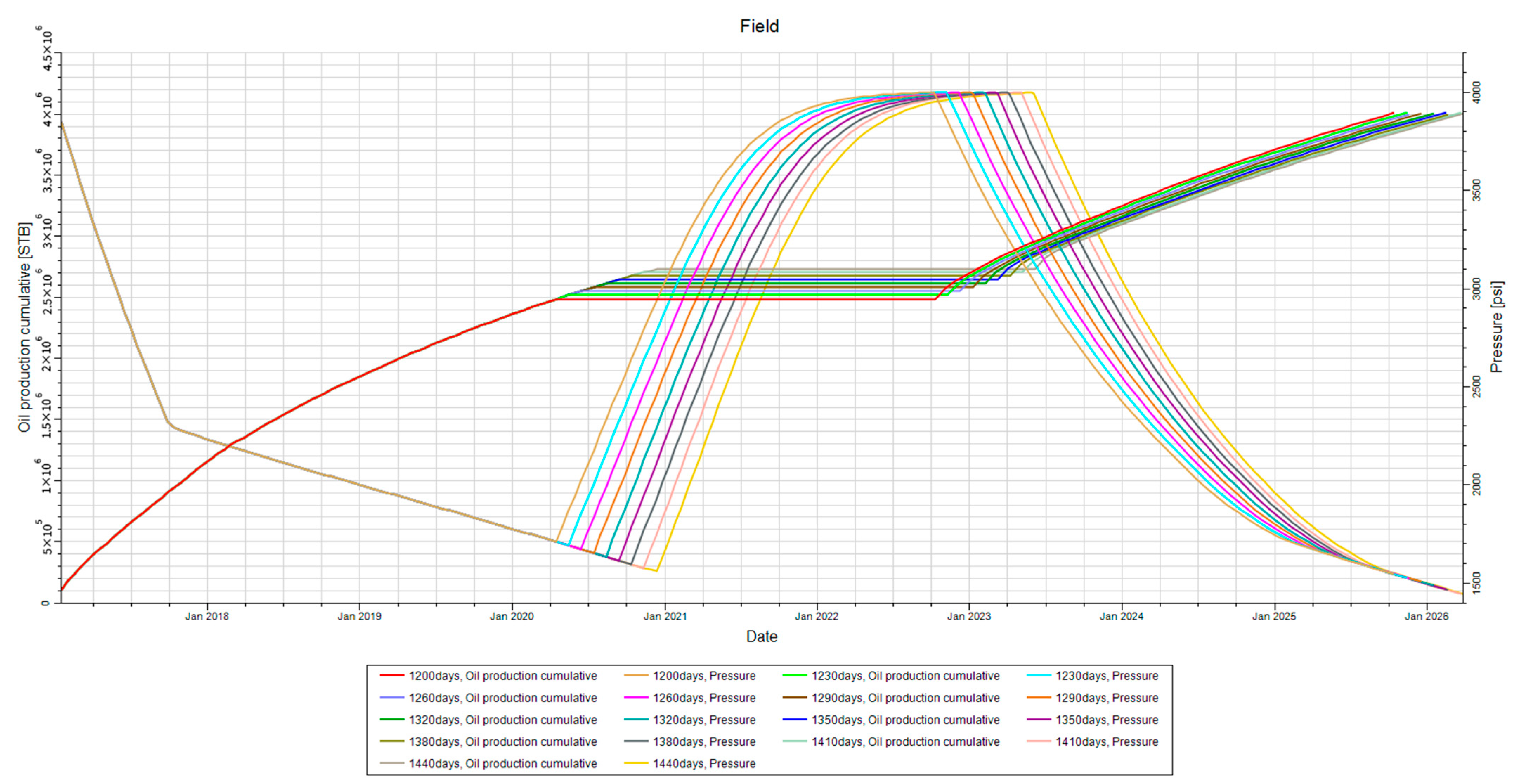
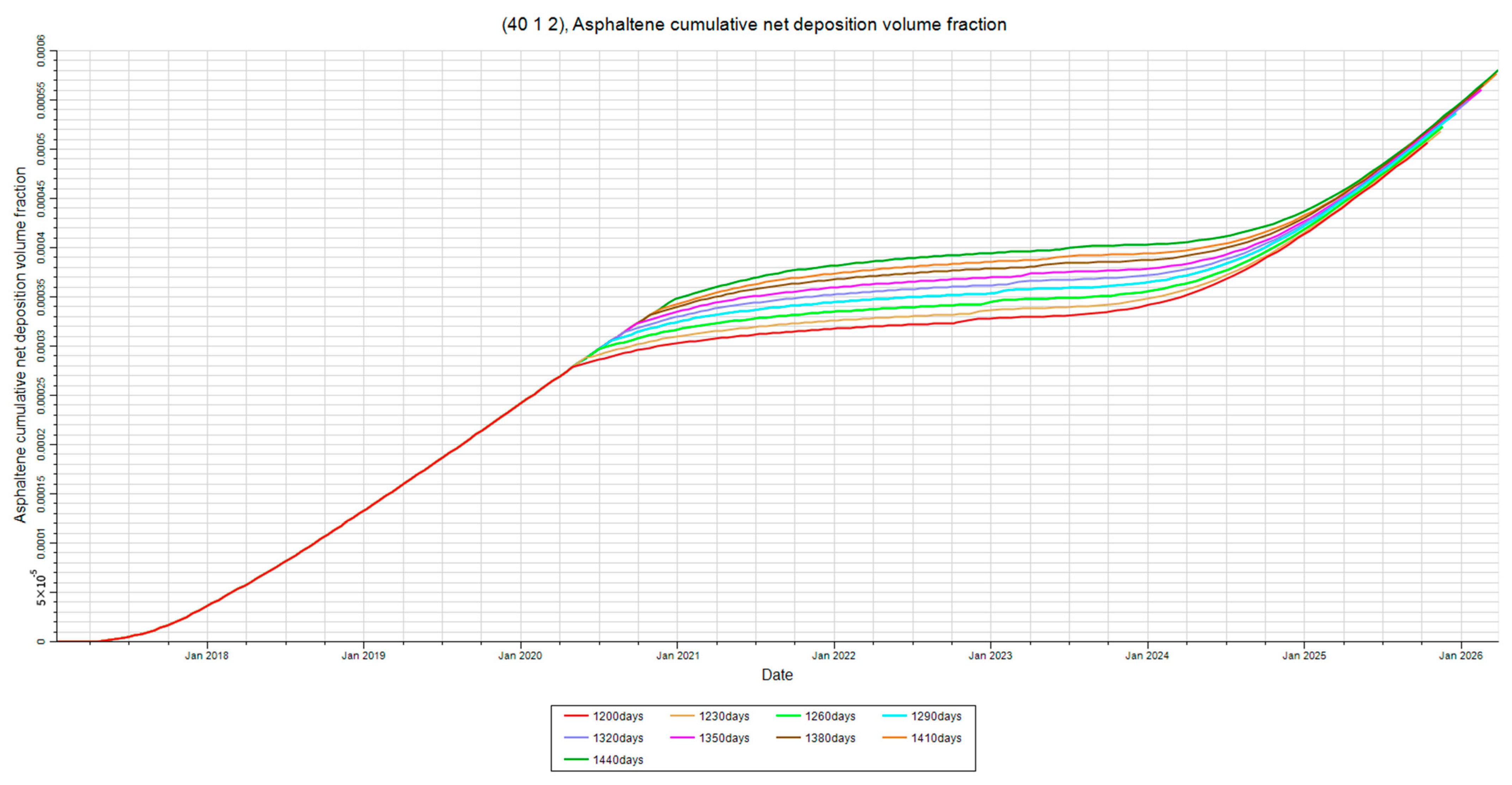
Figure 31 demonstrates how the simulation for the time of injection sensitivity analysis was conducted. The timing of water injection following primary depletion significantly affects asphaltene behavior due to evolving pressure and compositional dynamics. To evaluate this sensitivity, several cases were simulated with the injection start time varied by one-month increments, while maintaining a fixed one-week shut-in period and a maximum injection BHP of 4000 psi. All simulations were set to terminate after producing 4,000,000 stb of oil, ensuring uniform hydrocarbon withdrawal across cases.
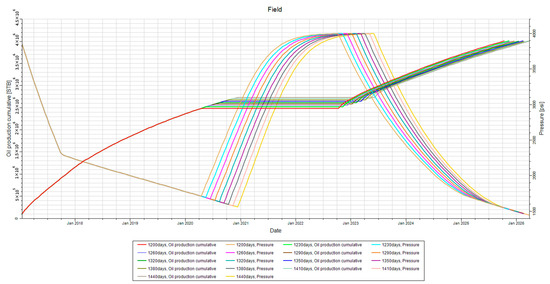
Figure 31.
Time of injection sensitivity. This figure illustrates how the injection time was varied for this analysis while keeping the cumulative produced oil constant.
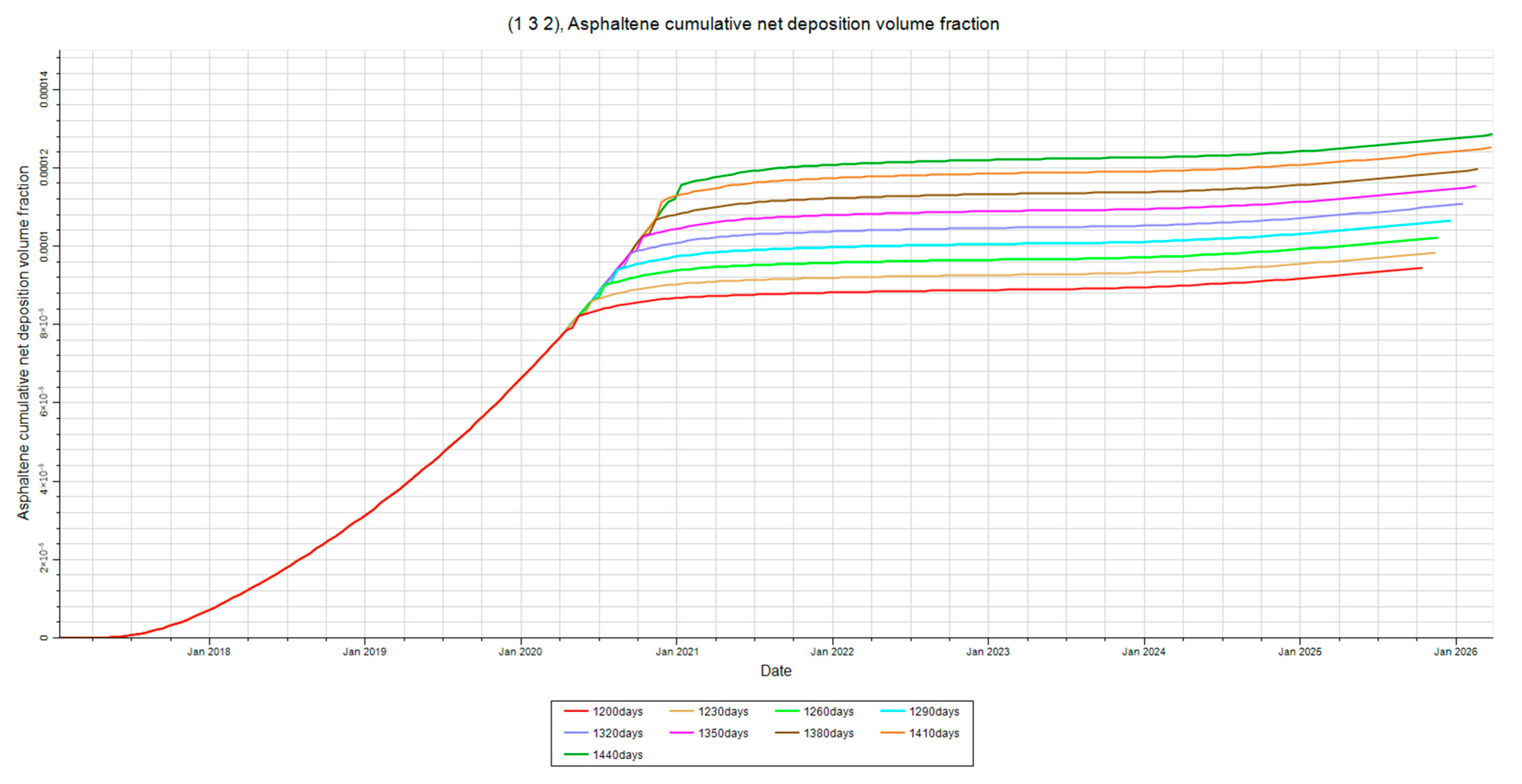
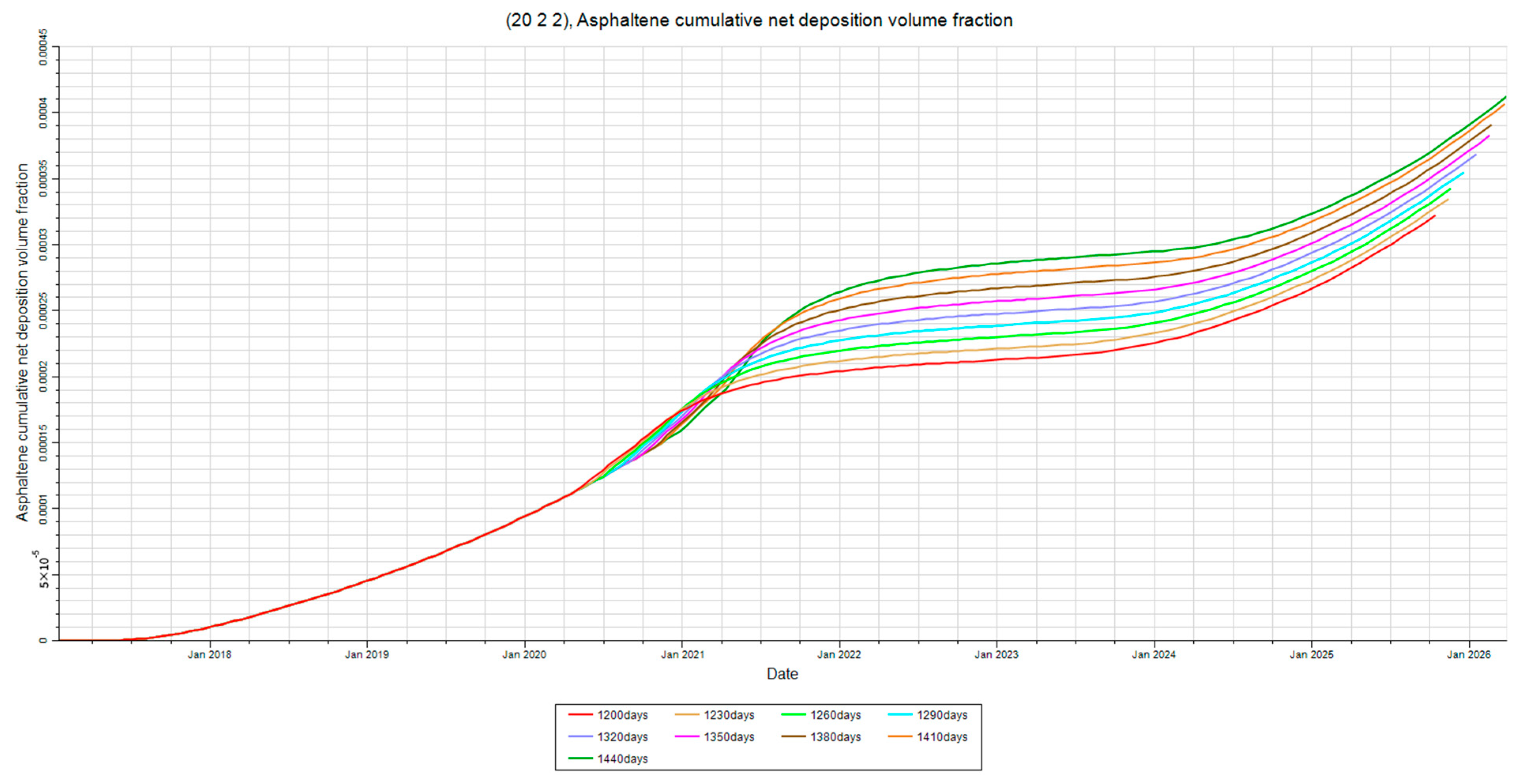
3.5.1. Deposition Behavior Across Injection Timing
Figure 32, Figure 33 and Figure 34 show that asphaltene deposition increases significantly with delayed injection. Longer primary depletion periods allow the reservoir pressure to fall further below the bubble point, destabilizing the oil phase. This causes an increase in flocculation rates due to both pressure-driven compositional changes and declining kinetic energy within the fluid system.
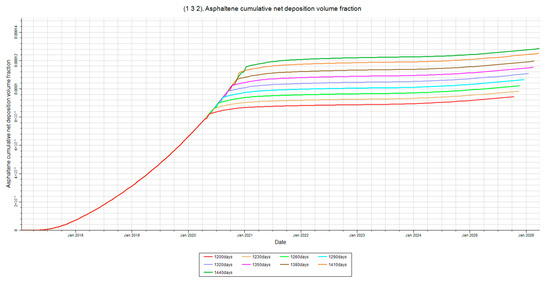
Figure 32.
Asphaltene deposition at the injector. This figure shows the asphaltene deposition at the injector in layer two for the injection time sensitivity analysis.
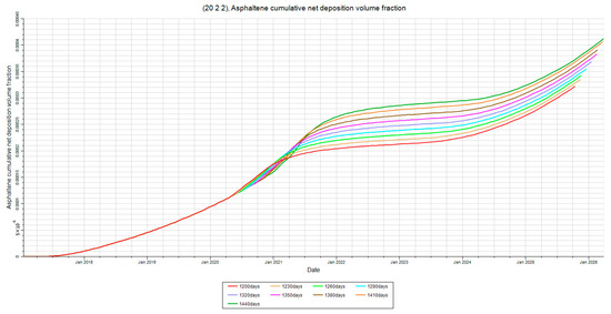
Figure 33.
Asphaltene deposition at mid-point. This figure shows the asphaltene deposition at the mid-point in layer two for the injection time sensitivity analysis.
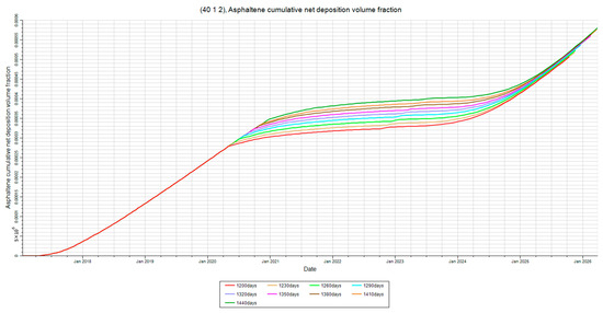
Figure 34.
Asphaltene deposition at the producer. This figure shows the asphaltene deposition at the producer in layer two for the injection time sensitivity analysis.
In early injection scenarios, the system is stabilized before significant colloid aggregation can occur, reducing net deposition. Conversely, when injection is delayed, more components critical to floc suspension (e.g., resins and light hydrocarbons) are lost, exacerbating deposition during the second production phase.
3.5.2. Mechanistic Interpretation and System Re-Stabilization
The observed behavior is governed by two key mechanisms:
- (1)
- Reservoir destabilization during depletion:
As pressure drops, kinetic energy decreases, and the crude loses its capacity to keep asphaltenes dispersed. Flocculation begins and escalates with time, especially near flow outlets like the producer.
- (2)
- Partial re-stabilization during water injection:
When injection begins, pressure restoration can re-dissolve non-deposited flocs, depending on how much destabilization has already occurred. However, this reversal is incomplete—largely due to thermal gradients and irreversible compositional changes. Early injection captures the reservoir in a less deteriorated state, allowing for better floc control.
These trends suggest that injection timing must be carefully optimized. Early waterflood initiation enhances system stability, minimizes deposition, and extends reservoir productivity, particularly in systems prone to asphaltene damage [19].
3.6. Comparison of Traditional W.F. to I.W.F. Effects on Asphaltene Damage
This section contrasts the performance of intermittent waterflooding (IWF) and traditional continuous waterflooding (WF) in mitigating asphaltene-related damage. The same reservoir model was used for both cases, with production constrained to 4,000,000 stb of oil to isolate deposition effects from cumulative recovery differences.
Figure 35 illustrates how the processes of the intermittent waterflood differs from that of the traditional waterflood. In the IWF case, operational parameters were optimized using results from prior sensitivity analyses (Section 3.1, Section 3.2, Section 3.3, Section 3.4 and Section 3.5). In contrast, the traditional WF scenario was modeled with continuous injection at a maximum BHP of 2000 psi, designed to maintain pressure and support displacement. This differential setup isolates the impact of re-pressurization dynamics unique to IWF from the steady-state pressure support in traditional WF.
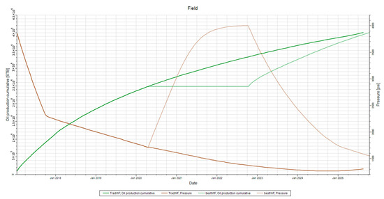
Figure 35.
Intermittent vs. traditional waterflood pressure and production. This figure highlights the differences between a traditional waterflood and an intermittent waterflood.
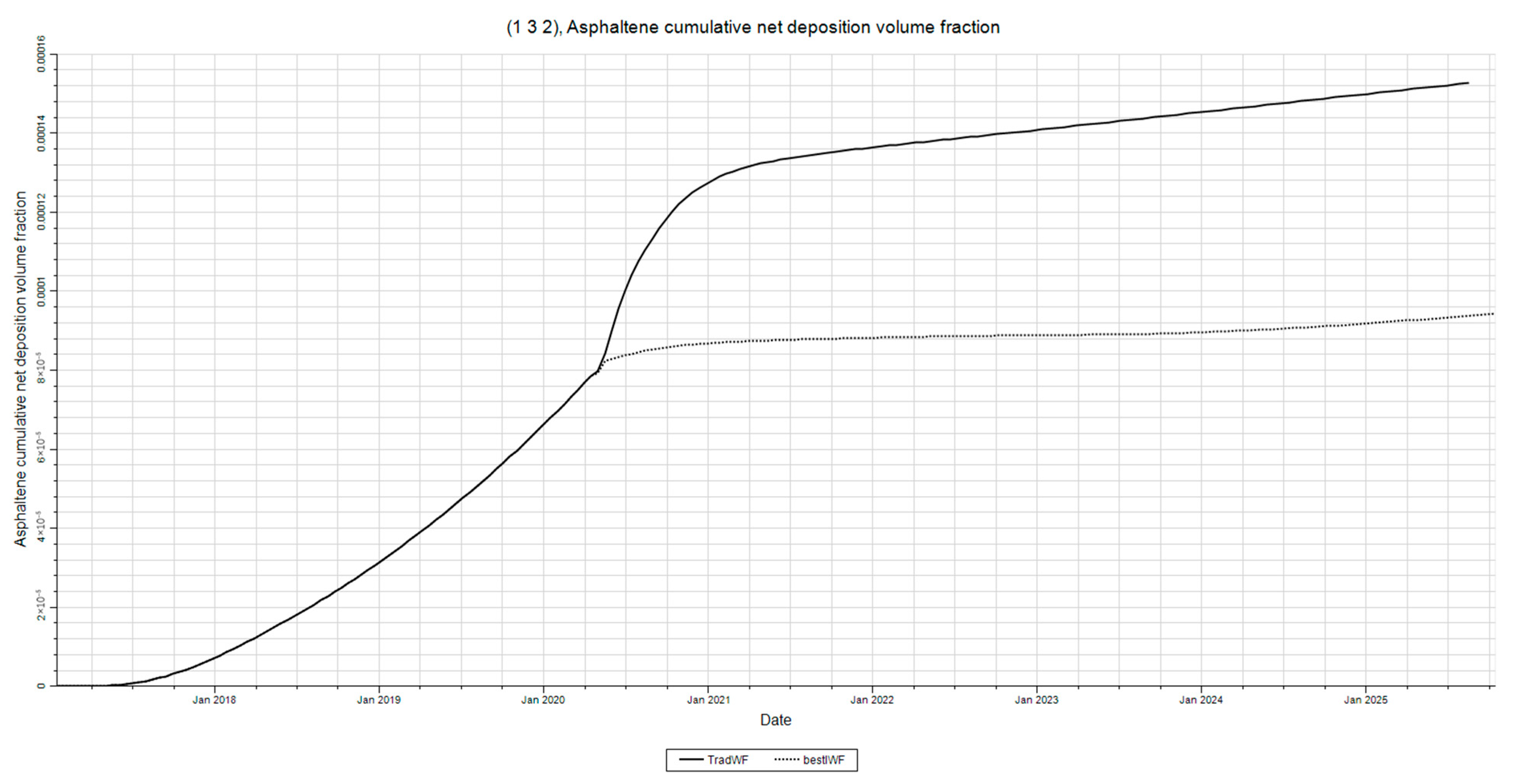
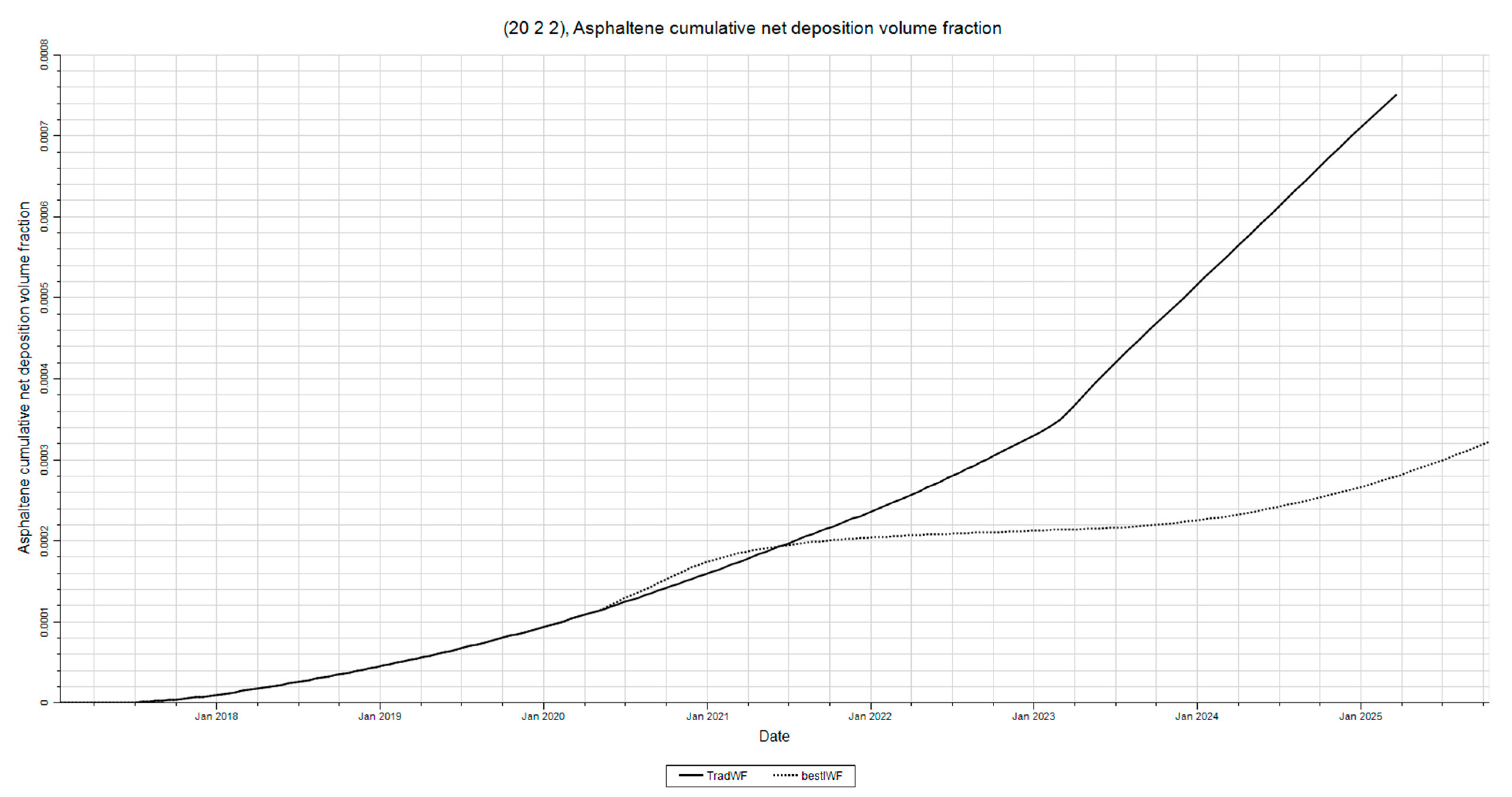
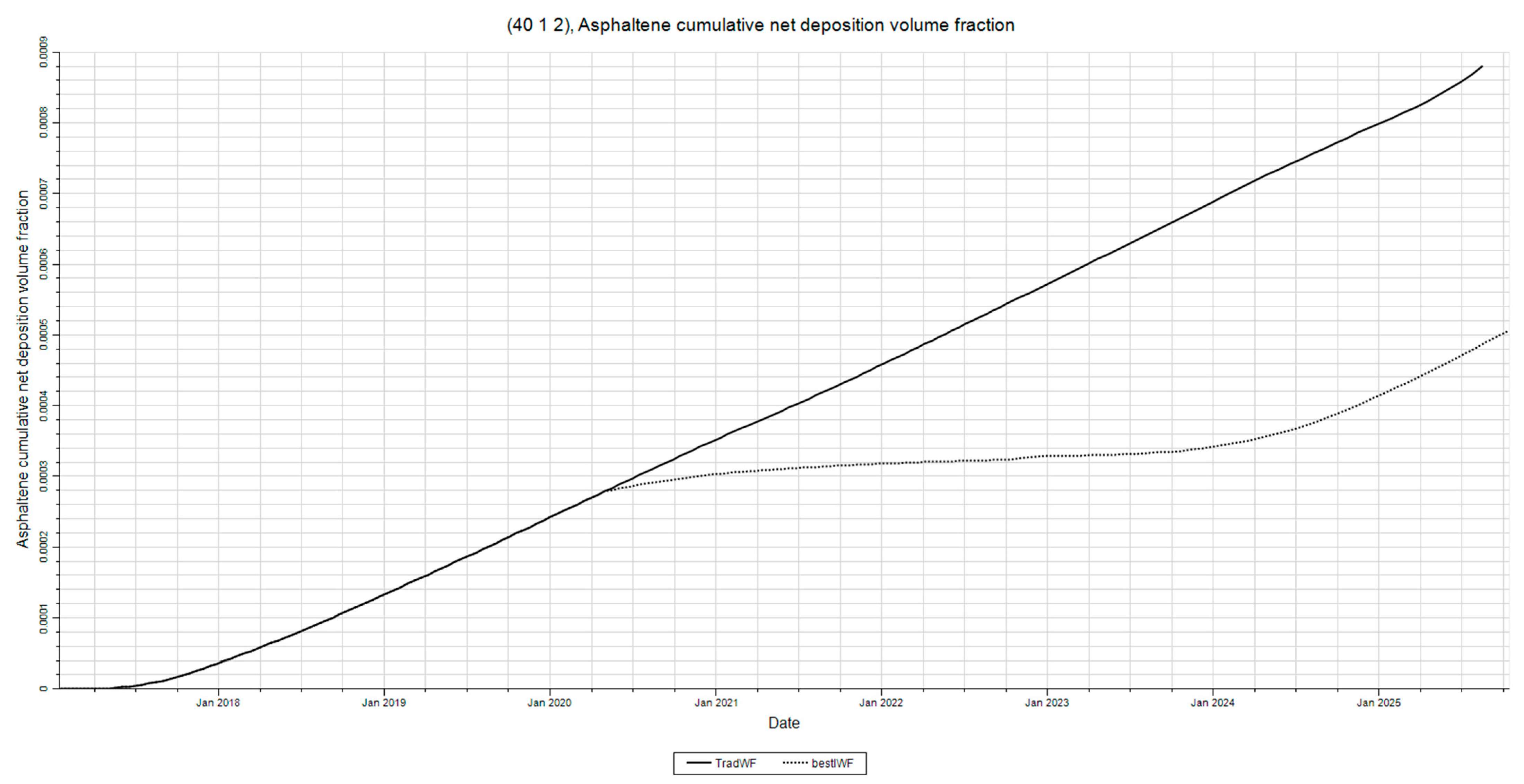
3.6.1. Deposition Comparison at Key Locations
Figure 36, Figure 37 and Figure 38 compare asphaltene deposition at the injector, midpoint, and producer. In all locations, IWF consistently demonstrates lower net deposition than traditional WF. This finding supports the hypothesis that periodic re-pressurization during IWF interrupts the flocculation-deposition cycle, allowing partial redissolution of suspended fines and reducing near-wellbore plugging.

Figure 36.
I.W.F. vs. traditional waterflood asphaltene deposition at the injector. This figure shows how I.W.F. can reduce asphaltene deposition at the injector.
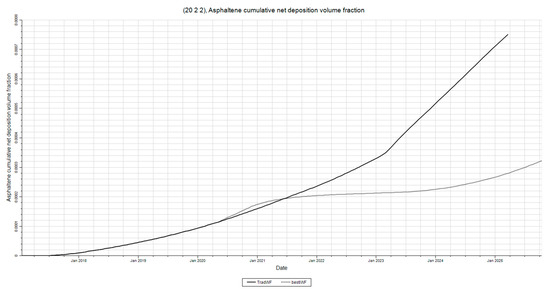
Figure 37.
I.W.F. vs. traditional waterflood asphaltene deposition at mid-point. This figure shows how I.W.F. can reduce asphaltene deposition at the mid-point.
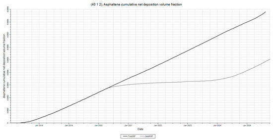
Figure 38.
I.W.F. vs. traditional waterflood asphaltene deposition at producer. This figure shows how I.W.F. can reduce asphaltene deposition at the producer.
Traditional WF, by contrast, maintains constant flow and temperature conditions that allow precipitation and flocculation to proceed unchecked once the destabilization threshold is reached. The lack of restabilization windows leads to higher cumulative damage.
3.6.2. Field Implications
The results validate IWF as an effective operational strategy to mitigate asphaltene deposition. The temporary shut-in periods enable the reservoir to partially re-equilibrate, especially in the near-producer region where drawdown and streamline convergence amplify deposition risks.
In field development planning, this approach can be particularly beneficial in reservoirs where asphaltene instability is a known risk or where continuous injection strategies have led to premature injectivity loss and plugging [20,21,22]. Implementing cyclic injection profiles, even short cycles, may enhance recovery while preserving permeability and flow assurance integrity [23].
4. Conclusions
This study demonstrates that intermittent waterflooding (IWF) can serve as an effective operational strategy to mitigate asphaltene deposition in oil reservoirs. Various sensitivity analyses were conducted using a compositional model in Eclipse 300 to evaluate how shut-in time, injection rate, and injection timing influence the extent and spatial distribution of asphaltene-related damage.
The key findings include
- (1)
- Shut-in time beyond a few days offers negligible additional benefit in reducing deposition, suggesting that extended reservoir idle periods delay recovery without significantly improving flow conditions.
- (2)
- Spatial trends show that the producer region consistently experiences the highest deposition, plugging, and permeability damage, largely due to pressure drawdown and streamline convergence.
- (3)
- Higher injection rates reduce near-wellbore deposition and shorten injection duration, offering both flow assurance and economic advantages.
- (4)
- Earlier injection timing helps stabilize the reservoir system before irreversible precipitation and flocculation occur, thereby minimizing cumulative damage.
- (5)
- Compared to traditional waterflooding, IWF substantially reduces asphaltene deposition at all key locations, particularly near the producer. This advantage is attributed to the re-pressurization phase that interrupts and reverses the flocculation-deposition cycle.
Collectively, the results support IWF as a practical, low-cost alternative to chemical mitigation strategies for managing asphaltene-related flow assurance risks. The findings also emphasize the importance of tailoring injection schedules to reservoir dynamics—particularly timing, pressure response, and phase behavior—to limit irreversible permeability loss and maximize oil recovery.
Supplementary Materials
The following supporting information can be downloaded at: https://www.mdpi.com/article/10.3390/pr13072143/s1, File S1: Data.
Author Contributions
Conceptualization, R.T. and H.T.; Writing—original draft, E.D.M.; Writing—review & editing, J.X., I.I. and N.O.; Supervision, F.B. All authors have read and agreed to the published version of the manuscript.
Funding
This research received no external funding.
Data Availability Statement
The data presented in this study are available in the Supplementary Material.
Conflicts of Interest
The authors declare no conflict of interest.
References
- Arunagiri, A.T.; Gnanasundaram, N.; Wilfred, C.D.; Rashid, Z.; Murugesan, T. A comprehensive review on recent advances in petroleum asphaltene aggregation. J. Pet. Sci. Eng. 2019, 176, 249–268. [Google Scholar] [CrossRef]
- Mohammed, I.; Mahmoud, M.; Al Shehri, D.; El-Husseiny, A.; Alade, O. Asphaltene precipitation and deposition: A critical review. J. Pet. Sci. Eng. 2020, 197, 107956. [Google Scholar] [CrossRef]
- Carrera, M.; Zarooni, M.; Olayiwola, O.; Nguyen, V.; Boukadi, F. Impacts of asphaltene deposition on oil recovery following a waterflood—A numerical simulation study. J. Pet. Chem. Eng. 2024, 2, 1–8. [Google Scholar] [CrossRef]
- Ghadimi, M.; Ghaedi, M.; Malayeri, M.R.; Amani, M.J. A new approach to model asphaltene induced permeability damage with emphasis on pore blocking mechanism. J. Pet. Sci. Eng. 2020, 184, 106512. [Google Scholar] [CrossRef]
- Fahes, M.; Abraham, J.; Mehana, M. The impact of asphaltene deposition on fluid flow in sandstone. J. Pet. Sci. Eng. 2019, 174, 676–681. [Google Scholar] [CrossRef]
- Khurshid, I.; Al-Attar, H.; Alraeesi, A.R. Modeling cementation in porous media during waterflooding: Asphaltene deposition, formation dissolution, and their cementation. J. Pet. Sci. Eng. 2018, 161, 359–367. [Google Scholar] [CrossRef]
- Qi, J.; Fan, C.; Li, S. Characteristics of lignite char derived from oxy-pyrolysis. Fuel 2021, 291, 120261. [Google Scholar] [CrossRef]
- Lo, P.A.; Tinni, A.O.; Milad, B. Experimental study on the influence of flow rate and pressure on the deposition of asphaltenes in a sandstone core sample. Fuel 2022, 310, 122420. [Google Scholar] [CrossRef]
- Stratiev, D.; Nikolova, R.; Veli, A.; Shishkova, I.; Toteva, V.; Georgiev, G. Mitigation of asphaltene deposit formation via chemical additives: A review. Processes 2025, 13, 141. [Google Scholar] [CrossRef]
- Shekarifard, A.; Shakib-Taheri, J.; Naderi, H. Experimental investigation of asphaltene deposition in porous media under ultrasonic and microwave fields. J. Pet. Sci. Eng. 2018, 163, 453–462. [Google Scholar] [CrossRef]
- Xiong, R.; Guo, J.; Kiyingi, W.; Li, Q. Method for judging the stability of asphaltenes in crude oil. ACS Omega 2020, 5, 23131–23140. [Google Scholar] [CrossRef] [PubMed]
- Tahernejad, E.; Bazvand, M.; Shadizadeh, S.R. Asphaltene Deposition Effects on Reservoir Rock Wettability and Permeability: An Experimental Study. Sci. Rep. 2024, 14, 15249. [Google Scholar] [CrossRef]
- Mehrabi, A.; Bagheri, M.; Nabi Bidhendi, M.; Delijani, E.B.; Behnood, M. Porosity estimation of carbonate reservoirs using a hybrid deep neural network model based on well data. Iran. J. Geophys. 2024, 18, 143–164. [Google Scholar] [CrossRef]
- Ali, S.I.; Lalji, S.M.; Haneef, J.; Tariq, S.M.; Junaid, M.; Ali, S.M.A. Determination of asphaltene stability in crude oils using a deposit level test coupled with a spot test: A simple and qualitative approach. ACS Omega 2022, 7, 14165–14179. [Google Scholar] [CrossRef] [PubMed]
- Saboor, A.; Yousaf, N.; Haneef, J.; Ali, S.I. Performance of asphaltene stability predicting models in field environment and development of a new predictor. J. Pet. Explor. Prod. Technol. 2022, 12, 1423–1436. [Google Scholar] [CrossRef]
- Moosavi, N.; Bagheri, M.; Nabi-Bidhendi, M. Hydrocarbon Reservoir Parameter Estimation Using a Fuzzy Gaussian Based SVR Method. Bull. Geophys. Oceanogr. 2024, 65, 1–14. Available online: https://bgo.ogs.it/sites/default/files/pdf/bgo00454_Moosavi.pdf (accessed on 24 May 2025).
- Hassanpouryouzband, A.; Joonaki, E.; Taghikhani, V.; Bozorgmehry Boozarjomehry, R.; Chapoy, A.; Tohidi, B. New two-dimensional particle-scale model to simulate asphaltene deposition in wellbores and pipelines. Energy Fuels 2018, 32, 2661–2672. [Google Scholar] [CrossRef]
- Mohebbinia, S.; Sepehrnoori, K.; Johns, R.T.; Kazemi Nia Korrani, A. Simulation of asphaltene precipitation during gas injection using PC-SAFT EOS. J. Pet. Sci. Eng. 2017, 158, 693–706. [Google Scholar] [CrossRef]
- Wang, S.; Civan, F. Preventing Asphaltene Deposition in Oil Reservoirs by Early Water Injection. In SPE Production Operations Symposium, Society of Petroleum Engineers; SPE: St Bellingham, WA, USA, 2005. [Google Scholar]
- Imqam, A.; Elturki, M. Experimental investigation of asphaltene deposition and aggregation in ultra-low permeability reservoirs under CO2 injection. In Proceedings of the SPE Canada Energy Technology Conference, Calgary, AB, Canada, 16–17 March 2022. SPE-208563-MS. [Google Scholar]
- Yin, D.; Li, Q.; Zhao, D. Investigating asphaltene precipitation and deposition in ultra-low permeability reservoirs during CO2-EOR. Sustainability 2023, 16, 4303. [Google Scholar] [CrossRef]
- Choiri, M.; Hamouda, A.A. Enhanced Oil Recovery by CO2 Flooding Effect on Asphaltene Stability Envelope and Compositional Simulation of Asphaltenic Oil Reservoir; SPE 141329; SPE: St Bellingham, WA, USA, 2011. [Google Scholar]
- Hussain, M.; Boukadi, F.; Hu, Z.; Adjei, D. Optimizing oil recovery: A sector model study of CO2-water-alternating-gas and continuous injection technologies. Processes 2025, 13, 700. [Google Scholar] [CrossRef]


Disclaimer/Publisher’s Note: The statements, opinions and data contained in all publications are solely those of the individual author(s) and contributor(s) and not of MDPI and/or the editor(s). MDPI and/or the editor(s) disclaim responsibility for any injury to people or property resulting from any ideas, methods, instructions or products referred to in the content. |
© 2025 by the authors. Licensee MDPI, Basel, Switzerland. This article is an open access article distributed under the terms and conditions of the Creative Commons Attribution (CC BY) license (https://creativecommons.org/licenses/by/4.0/).