Abstract
Accurate prediction of key environmental parameters is crucial for intelligent control and optimization, yet it remains challenging due to gradient instability in deep learning models, like Long Short-Term Memory (LSTM), during time series forecasting. This study introduces a novel adaptive optimization algorithm, NadamClip, which integrates gradient clipping directly into the Nadam framework to address the trade-off between convergence efficiency and gradient explosion. NadamClip incorporates an adjustable gradient clipping threshold strategy that permits manual tuning. Through systematic experiments, we identified an optimal threshold range that effectively balances model performance and training stability, dynamically adapting to the evolving convergence characteristics of the network across different training phases. Aquaculture systems are regarded as similar to modern biomanufacturing systems. The study evaluated an aquaculture dataset for ammonia concentration prediction in aquaculture environmental control processes. NadamClip achieved outstanding results on key metrics, including a Root Mean Square Error (RMSE) of 0.2644, a Mean Absolute Error (MAE) of 0.6595, and a Coefficient of Determination (R2) score of 0.9743. Compared to existing optimizer enhancements, NadamClip pioneers the integration of gradient clipping with adaptive momentum estimation, overcoming the traditional paradigm where clipping primarily serves as an external training control rather than an intrinsic algorithmic component. This study provides a practical and reproducible optimization framework for intelligent modeling of dynamic process systems, thereby contributing to the broader advancement of machine learning methods in predictive modeling and optimization for data-driven manufacturing and environmental processes.
1. Introduction
The growing global demand for efficient and sustainable production systems has heightened the requirements for real-time prediction and control of key parameters in biologically based, environmentally driven systems, such as water treatment and fermentation reactors. Ammonia is a common metabolic byproduct in water. Fluctuations in its concentration can significantly compromise system stability under conditions of elevated temperature and high pH. Furthermore, ammonia can generate secondary pollutants, such as nitrite, through nitrification processes, thereby degrading process performance [1]. Traditional physical and chemical models struggle to capture the dynamic variations in ammonia concentration, which are driven by the complex interplay of biological excretion, environmental disturbances, and nonlinear metabolic transformations [2]. Consequently, there is a pressing need for deep-learning-based time series prediction methods to enhance the accuracy and robustness of parameter monitoring.
In recent years, Long Short-Term Memory networks (LSTM) have been widely applied to ammonia concentration prediction due to their strong time series modeling capabilities [3]. However, LSTM training relies on stochastic gradient descent (SGD) and its variants (e.g., Adam, Nadam) for parameter optimization, making it susceptible to gradient explosion—where excessive gradient accumulation during backpropagation leads to severe parameter oscillations, causing training instability and entrapment in local optima [4]. Gradient clipping is a widely used technique in deep neural network training, primarily employed to prevent gradient explosion and enhance training stability [5]. In recent years, researchers have directly embedded clipping techniques into various SGD algorithms and their variants to improve the robustness of the optimization process.
In standard SGD, Marshall et al. suppressed gradient fluctuations in high-dimensional linear regression through fixed-threshold clipping [6]. In Momentum SGD, Mai and Johansson introduced a clipping mechanism into the momentum update procedure, ensuring stable convergence in non-smooth scenarios [7], while Zhang et al. achieved clipping-equivalent effects through normalization operations [8].
For adaptive optimizers, Chezhegov et al. embedded clipping into the updates of AdaGrad and Adam, effectively enhancing convergence performance under heavy-tailed noise [8]. Seetharaman et al. proposed AutoClip, which dynamically sets clipping thresholds and is compatible with optimizers like Adaptive Moment Estimation (Adam) and Root Mean Square Propagation (RMSProp) [9] In distributed SGD, Liu et al. integrated clipping into local updates, improving communication efficiency and stability [10]. In Differentially Private SGD (DP-SGD), Tang et al. balanced privacy protection and training performance through per-sample clipping [11]. Additionally, Qian et al. demonstrated clipping’s effectiveness in controlling fluctuations within incremental SGD [12], while Ramaswamy et al. proposed a unified modeling framework for clipping [13].
Although these methods have achieved some success in enhancing the performance of optimization algorithms, they are inherently constrained by the stochastic gradient descent (SGD) framework, which typically lacks the integration of the Nesterov momentum mechanism. This limitation hinders their ability to effectively balance gradient trend prediction with training stability, thereby imposing constraints when tackling complex, non-convex problems. Within this context, Nesterov-accelerated Adaptive Moment Estimation (Nadam), which incorporates the Nesterov momentum mechanism into the adaptive learning rate framework of Adam, demonstrates faster convergence rates and enhanced update foresight [14]. However, existing research has yet to explore the explicit integration of gradient clipping techniques within the Nadam optimizer itself. This gap presents a promising research direction for further improving training stability and generalization capability. Therefore, this study aims to develop and validate an enhanced optimization algorithm, NadamClip, which integrates the gradient clipping mechanism into the Nadam optimizer, with the goal of improving the stability and accuracy of complex time series prediction tasks.
This paper first introduces the developmental background of gradient clipping technology and its current application status in various stochastic gradient descent algorithms in the Introduction section. It explicitly proposes integrating a clipping mechanism into the Nadam optimizer to enhance the training stability and convergence efficiency of LSTM models for ammonia nitrogen prediction in aquaculture. Subsequently, Section 2 details the construction process of the NadamClip algorithm, provides theoretical proofs of its correctness and stability, and describes the experimental design and parameter settings. Section 3 validates the effectiveness of NadamClip through comparative experiments with multiple optimization algorithms and analyzes the results. Finally, Section 4 presents the discussion, and Section 5 concludes the paper and outlines future research directions.
2. Materials and Methods
2.1. Proposed Algorithm
The NadamClip algorithm embeds a gradient clipping mechanism directly within the Nadam optimizer. It not only preserves the advantages of Nadam’s Nesterov momentum and adaptive learning rate [15] but also dynamically constrains gradient magnitudes in real time via an adjustable clipping threshold. This effectively prevents parameter oscillations caused by gradient explosions during training. This approach transcends conventional limitations that treat gradient clipping as an external operation, establishing for the first time a deeply integrated, unified framework where clipping is intrinsically coupled with the Nadam optimizer’s internal mechanisms. Consequently, it enhances training stability and convergence efficiency. This integrated design enables more precise and dynamic gradient control, significantly improving model optimization performance in non-stationary environments.
2.1.1. Nadam Formula
Nadam (Nesterov-accelerated Adaptive Moment Estimation) is an optimization algorithm that combines the adaptive learning rate mechanism of Adam with the lookahead gradient approach of Nesterov accelerated gradient (NAG). While traditional momentum methods adjust parameter updates based on accumulated gradients from previous steps, Nesterov momentum anticipates future gradient directions, enabling more informed updates. Nadam integrates this foresight into Adam’s adaptive update framework, allowing parameters to converge more efficiently toward optimal solutions [14].
This integration leads to faster convergence and improved stability during training, especially in non-convex optimization problems or when dealing with noisy gradients. Compared to the original Adam optimizer, Nadam is more effective in mitigating oscillations and often shows better performance in the early stages of training. In various deep learning tasks, Nadam has been observed to outperform standard momentum methods, RMSProp, and Adam, particularly when handling sparse features or complex network architectures [16]. As a result, Nadam has been widely adopted as an enhanced optimizer in neural network training, playing a significant role in improving training efficiency and overall model performance [17]. To enhance clarity and preserve the structural presentation of the original Nadam algorithm as proposed by Dozat (2016) [14], its complete workflow is organized in Algorithm 1.
| Algorithm 1: Nesterov-accelerated Adaptive Moment Estimation (Nadam) |
|
Hyperparameters (first/second moment vectors) not converged do end while |
Learning rate at time step ttt; it controls the step size during parameter updates. A common value is 0.001.
: Exponential decay rate for the first moment estimates (similar to β1 in Adam, typically around 0.9); it determines how much past gradients influence the current moment estimate.
: Exponential decay rate for the second moment estimates (similar to β2 in Adam, often close to 0.999); it smooths the squared gradients.
A small constant added to the denominator for numerical stability (usually 10−8).
t: The maximum number of training steps or iterations (used to denote the training horizon or the step index limit).
: The gradient of the loss function with respect to parameters at time step t.
: The first moment estimate (i.e., the exponential moving average of past gradients) at time step t, initialized to 0.
: The second moment estimate (i.e., the exponential moving average of squared gradients) at time step t, initialized to 0.
Bias-corrected estimate of the first moment, combining the exponential average and the current gradient in a Nesterov-style lookahead.
: Bias-corrected estimate of the second moment.
: The model parameters at time step t.
2.1.2. Gradient Clipping
Standard gradient clipping constrains gradient magnitudes to maintain training stability at the cost of introducing estimation bias. U-Clip improves this paradigm through a dynamic buffering mechanism that retains clipped gradient components and strategically reapplies these residual values to subsequent gradient updates [18]. This design ensures constrained cumulative update deviations while achieving long-term unbiased optimization, thereby simultaneously enhancing training stability and convergence efficiency. The bias mitigation properties of U-Clip in stochastic gradient clipping are mathematically demonstrated through Equations (1)–(5):
For , coordinate clipping to scale γ > 0 is given by
Introduction of U-Clip:
Gradient clipping:
Update buffer: 4.1
where is the updated buffer.
Parameter update:
: Gradient
Gradient clipping threshold, limiting the maximum value of the gradient. You can choose a fixed value, such as 0.5.
A buffer that holds the gradient that was clipped in the previous steps.
: The gradient after clip function processing.
: Learning rate, control parameter update step size. Usually, the learning rate value can be 0.01 or 0.001.
: Weights and biases need to be trained.
2.1.3. Proposed New Algorithm
This section proposes a new algorithm, NadamClip. The NadamClip algorithm performs an error-compensated gradient clipping operation during each iteration. Its core innovation lies in applying clipping not directly to the raw gradient, , but to the composite gradient modified through historical compensation. The clipping operation scales the composite gradient via the scaling factor , generating the effective gradient UtUt while simultaneously calculating the truncated gradient component . This component propagates as error compensation to subsequent iterations. This design uniquely positions gradient clipping before momentum updates, enabling clipping operations to directly influence the momentum system’s evolutionary trajectory.
During the momentum update phase, the algorithm employs a dual-channel mechanism for gradient processing. The first-moment vector mtmt integrates historical momentum and clipped gradient through exponential moving averaging, while the second-moment vector smooths with an independent decay rate . This decoupled treatment allows the adaptive learning rate mechanism to accurately capture the statistical properties of clipped gradients. The critical bias correction step exhibits an innovative dual-component structure: The corrected momentum simultaneously incorporates the immediate contribution of the current clipped gradient (weighted by ) and a forward-looking projection of the future momentum decay coefficient (implemented via Nesterov acceleration), creating a unique temporal fusion. In contrast, the second-moment correction applies conventional scaling.
Finally, during parameter updating, the algorithm combines the corrected momentum with the adaptive learning rate to determine the update direction. This mechanism exhibits fundamental structural differences from conventional optimizers. First, gradient clipping precedes momentum computation, enabling the momentum system to receive norm-constrained gradients that suppress gradient explosion propagation at the source. Second, the error compensation term propagates residual clipping information across iterations, preserving and rectifying gradient information throughout the update chain to enhance long-term training consistency and robustness. Finally, the Nesterov acceleration mechanism within the momentum correction step incorporates forward-looking information via the future momentum decay coefficient , strengthening momentum path regulation to significantly improve optimization responsiveness and dynamic adaptability. The NadamClip algorithm formula is presented in Algorithm 2.
| Algorithm 2: Nesterov-accelerated Adaptive Moment Estimation Clipping (NadamClip) |
|
Hyperparameters (clipping region) (first/second moment vectors) not converged do end while |
: The maximum number of training steps or iterations (used to denote the training horizon or step index limit).
: The gradient of the loss function with respect to parameters at time step t.
: The model parameters at time step t.
: The gradient after clip function processing.
Gradient clipping threshold, limiting the maximum value of the gradient. You can choose a fixed value, such as 0.5
A buffer that holds the gradient that was clipped in the previous steps.
: The first moment estimate (i.e., the exponential moving average of past gradients) at time step t, initialized to 0.
: Exponential decay rate for the first moment estimates (similar to β1 in Adam, typically around 0.9); it determines how much past gradients influence the current moment estimate.
: The second moment estimate (i.e., the exponential moving average of squared gradients) at time step t, initialized to 0.
: Exponential decay rate for the second moment estimates (similar to β2 in Adam, often close to 0.999); it smooths the squared gradients.
Bias-corrected estimate of the first moment, combining the exponential average and the current gradient in a Nesterov-style lookahead.
: Bias-corrected estimate of the second moment.
Learning rate at time step ttt; it controls the step size during parameter updates. A common value is 0.001.
A small constant added to the denominator for numerical stability (usually 10−8).
The core operational logic of NadamClip involves calculating gradient norms during each training iteration and applying truncation or scaling operations when norms exceed predefined thresholds, thereby constraining maximum gradient magnitudes to prevent explosion phenomena. The system continuously monitors peak gradient norms throughout the training phase, records these values at epoch completion, and utilizes them as empirical baselines for adaptive threshold calibration. By evaluating MAE, RMSE, and R2 performance across multiple threshold configuration, the optimal dynamic threshold range was determined to balance model accuracy with gradient stability. This methodology not only prevents overemphasis on transient gradient patterns but also ensures stable parameter update consistency, ultimately accelerating LSTM convergence rates while improving prediction fidelity. This mathematical formula derivation analysis confirms that NadamClip maintains the adaptive learning advantages of Nadam while incorporating gradient norm constraints, providing both theoretical guarantees and practical stability for optimization in high-variance scenarios. For completeness, the full proof of formula correctness is provided in Appendix A.
2.2. Experimental Setup
To empirically verify the theoretical basis of NadamClip, we adopted a structured experimental protocol, including data collection and preprocessing, model setup, specified architecture configuration, baseline optimizer parameters, and gradient clipping threshold range experimental design. The platform used for these experiments was Google Collaboratory (Colab). The studies utilized the v2-8 Tensor Processing Unit (TPU), comprising eight TPU cores. TensorFlow version 2.15.0, which provides a comprehensive framework for building and deploying machine learning models, improves usability and interacts with Keras to accelerate model building and experimentation [18].
2.2.1. Data Collection and Preprocessing
In aquaculture environments, ammonia generation and accumulation are influenced by multiple water quality parameters, with water temperature (TP), dissolved oxygen (DO), and pH value being the primary influencing factors. Ammonia primarily originates from the decomposition of nitrogen-containing organic matter in water bodies and the metabolic excretion of fish, existing in two forms: free ammonia (NH3) and ammonium ions (NH4+). The transformation between these two forms is strongly regulated by temperature and pH. Specifically, elevated temperatures and higher pH values promote the conversion of NH4+ into the more toxic NH3, consequently increasing ammonia toxicity risks. Furthermore, dissolved oxygen levels serve as indicators of water self-purification capacity and nitrogen cycle activity. Under low DO conditions, impaired nitrification processes lead to accelerated ammonia accumulation.
Consequently, this study employs a primary dataset from a single aquaculture pond in Kaggle, comprising temperature, dissolved oxygen, pH, and ammonia measurements. This IoT-tagged dataset, compiled for aquaculture water quality monitoring, was collected by the HiPIC Research Group at the Department of Computer Science, Nsukka University, Nigeria. Funded through the 2020 Lakuna Prize for Agriculture in sub-Saharan Africa and administered via the Meridian Institute in Colorado, USA, the dataset contains sensor-recorded aquaculture pond measurements spanning June to mid-October 2021.
The dataset contains 83,127 entries available through the Sensor-Based Aquaponics Fish Pond Dataset. Optimal aquaculture conditions maintain temperatures between 20 and 30 °C, dissolved oxygen levels at 5–8 mg/L, and pH values within 6.5–8.5. Safety thresholds are defined as <0.2 mg/L for chronic total ammonia exposure and 2.9–5.0 mg/L for acute toxicity limits. Representative data samples are shown in Table 1.

Table 1.
Sample of dataset P1.
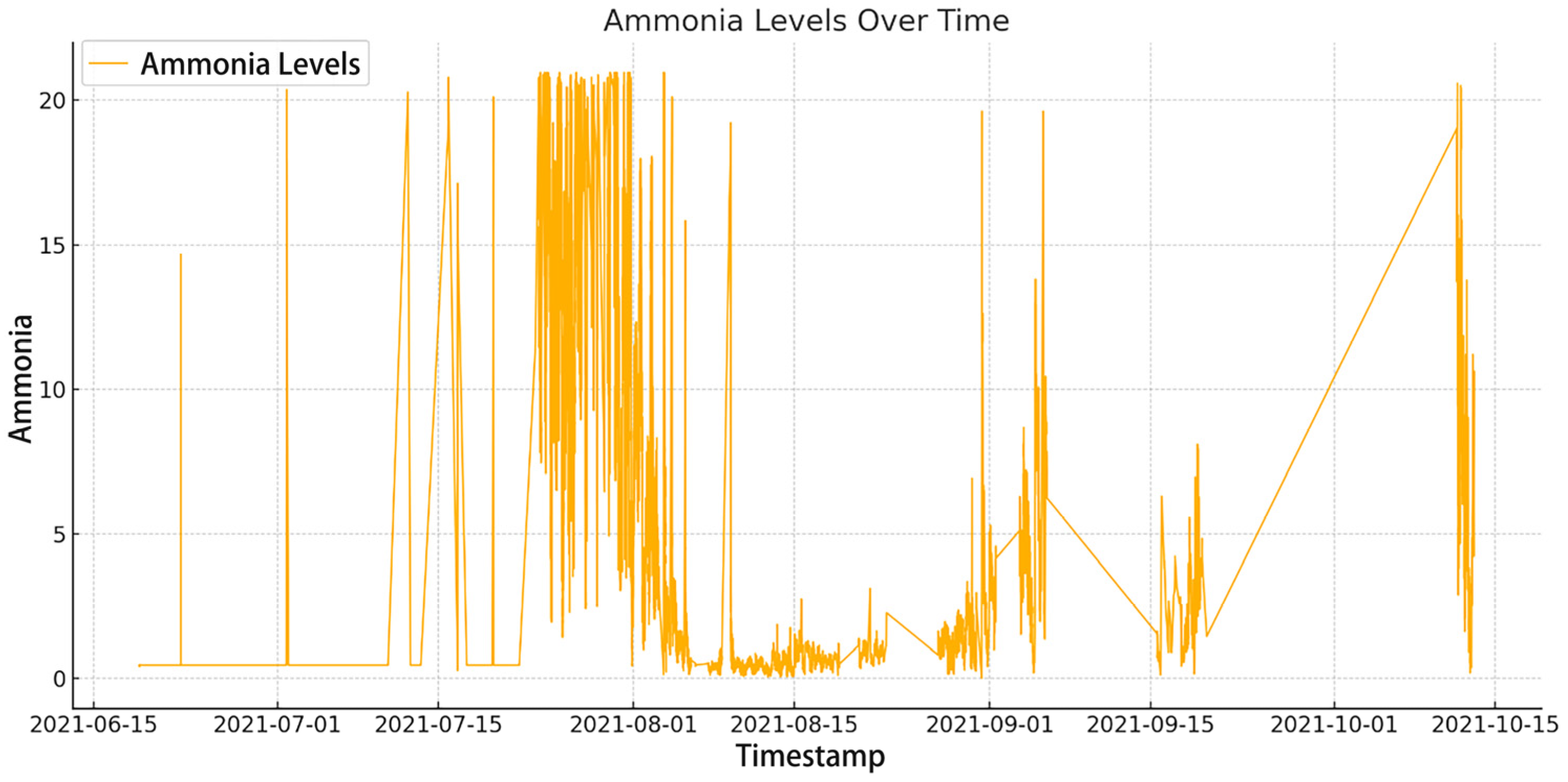
The Figure 1 visualizes the data of ammonia.

Figure 1.
P1 dataset ammonia visualization.
Figure 1 illustrates continuous ammonia concentration monitoring over time, with the horizontal axis (X-axis) corresponding to the temporal dimension and the vertical axis (Y-axis) depicting ammonia levels. The fundamental characteristic of this time series data lies in its chronological observation sequence. Each plotted point corresponds to a specific timestamp, demonstrating the inherent temporal dependency of ammonia concentration measurements—a critical attribute enabling effective LSTM model training.
- Data Correlation Analysis
To systematically investigate the temperature, dissolved oxygen, and pH effects on ammonia prediction, we performed correlation analysis of historical data to establish statistical foundations for deep-learning-based prediction model development. The Pandas corr() method was employed to quantify inter-variable correlation coefficients, with results presented in Figure 2.
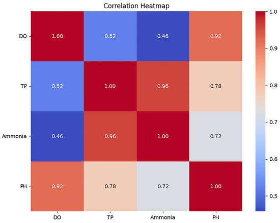
Figure 2.
Heat map of variable correlations.
The analysis revealed the strongest positive correlation between temperature and ammonia concentration (r = 0.96), demonstrating that thermal variations exerted significant effects on ammonia dynamics. Dissolved oxygen showed moderate positive correlation with ammonia (r = 0.46), reflecting its indirect role in redox-mediated processes rather than direct ammonia regulation. pH demonstrated substantial correlation with ammonia levels (r = 0.72), highlighting its critical influence on ammonia speciation. These robust correlations collectively explain 83% of ammonia concentration variability (R2 = 0.83), establishing temperature, dissolved oxygen, and pH as essential predictors for ammonia forecasting models in aquaculture systems.
- 2.
- Data Normalization
The quality of the data utilized by machine learning algorithms dictates their efficacy. Consequently, data preparation techniques, such as data normalization, are essential for normalizing the values of input and output variables to a defined range. This inquiry will utilize Min Max Normalization, with its definition presented in Formula (1).
The results of normalization are presented in Table 2.
Table 2.
Sample table for data normalization process.
Through the above data collection and preprocessing steps, this paper ensures the integrity and quality of the input data of the model.
2.2.2. Model Settings
Prior to hyperparameter optimization, the dataset underwent stratified partitioning with an 80:20 ratio between training–validation and test subsets. The training–validation set was further divided using identical proportions, resulting in final allocations of 64% training data (10,278 samples), 16% validation data (12,847 samples), and 20% test data. This tripartite division ensured rigorous separation for model training, hyperparameter validation, and final performance evaluation. The hyperparameter search process implemented a hybrid stochastic search with 3-fold cross-validation, systematically evaluating 100 unique parameter configurations per fold through 300 total model fittings. Experimental results demonstrated significant performance variance across parameter combinations, with the optimal configuration (Table 3) achieving superior balance between training efficiency and predictive accuracy.
Table 3.
Results of hyperparameter optimization.
The optimized architecture consists of two stacked LSTM layers with 144 and 124 units, respectively. Empirical evaluations demonstrate that a learning rate of 0.001 prevents overfitting through controlled parameter updates while enhancing generalization performance. A batch size of 32 was found to optimize computational efficiency while maintaining model convergence stability.
2.2.3. Gradient Clipping Threshold Range Design
Gradient clipping serves as a critical stabilization mechanism in deep learning, effectively mitigating gradient explosion risks while ensuring training process continuity [19]. This fundamental principle operates through threshold-based gradient regulation; when gradients exceed predefined thresholds, the algorithm systematically rescales excessive gradients to maintain update stability through constrained parameter adjustments [7]. Optimal threshold selection requires empirical determination via hyperparameter optimization—a critical process balancing convergence speed with update precision to maximize model performance.
This study conducted a systematic experiment to examine the effects of various thresholds on training loss, validation loss, and other metrics (refer to experimental Table 4), aiming to determine the optimal threshold range for mitigating gradient anomalies. This approach significantly reduces the cost of trial and error, enhances model convergence stability, maximizes the efficiency of gradient information utilization, and provides reliable training assurance for complex tasks.
Table 4.
Proposed gradient range setting.
The experiment began by establishing a high initial gradient threshold (no clipping applied) while simultaneously recording the original gradient norms and model performance metrics (RMSE, MAE, R2). The threshold was progressively decreased with defined step sizes (0.05–0.1), and performance fluctuations during retraining under each adjusted threshold were systematically recorded. Through multiple iterations, the critical threshold range associated with significant performance improvement was identified, after which the step size was refined (0.01–0.005) within this interval to determine the optimal threshold. This ideal threshold was required to simultaneously reduce RMSE/MAE, maximize R2, and ensure both training stability and convergence efficiency. The threshold’s effectiveness in controlling gradient explosion and preventing overfitting was confirmed through multiple validation cycles, thereby improving the model’s generalization capability.
2.2.4. Performance Metrics
This proposed study will employ three performance evaluation measures to assess the efficacy of the upgraded NadamClip algorithms across various datasets. This proposed study depends on the analysis of time series data, making it essential to highlight the importance of utilizing an appropriate assessment metric. The choice of a suitable evaluation metric is of utmost importance, as it justifies the anticipated outcomes. This study used MAE, RMSE, and R2 as measures for performance evaluation. MAE quantifies the average absolute magnitude of the error between expected and actual values, thus illustrating prediction accuracy. RMSE quantifies the root mean square of prediction errors, highlighting the influence of bigger errors on model efficacy. R2 is utilized to evaluate the degree to which the model accounts for the variability in the dependent variable, reflecting the model’s goodness of fit [20]. The performance evaluation index formulas of MAE, RMSE, and R2 are shown in Formulas (7), (8), and (9), respectively [21].
This study will conduct a comparative experimental analysis to systematically evaluate the effectiveness of the NadamClip optimizer in the LSTM architecture for predicting ammonia concentrations in aquatic environments. The investigation maintained methodological consistency by employing standardized datasets (uniformly pre-processed and partitioned) with identical initialization parameters, benchmarking NadamClip against Adam, SGD, RMSprop, and clipping-enhanced variants, including SGD-Clip [22]. Gradient clipping thresholds were systematically varied to quantify their influence on training stability (gradient explosion suppression) and prediction metrics (RMSE, MAE [23], R2 [24]), thereby identifying optimal threshold boundaries. All experimental trials rigorously documented hyperparameter configurations, training protocols, and performance outcomes to ensure cross-method comparability, enabling comprehensive evaluation of NadamClip’s synergistic advantages in accelerating model convergence, enhancing prediction precision, and strengthening generalization capacity.
3. Results
Building on the proposed algorithm and its theoretical foundations, this section presents experimental results to evaluate the optimization performance and practical effectiveness of the NadamClip method.
3.1. Model Training
The following is the LSTM model trained by the NadamClip algorithm. The hyperparameters of all training are unified, and the number of training iterations is 100.
3.1.1. Initial Training
The subsequent experimental phase evaluates the true efficacy of the NadamClip algorithm by setting an appropriate gradient clipping threshold for comparison and demonstrating the model’s optimization performance within a suitable gradient range.
When the gradient clipping threshold is set to 100, the gradient remains untrimmed. After completing 100 training iterations, the model’s performance is evaluated, with the results presented in Table 5.
Table 5.
Training Model Evaluation Results with Gradient Threshold of 100.
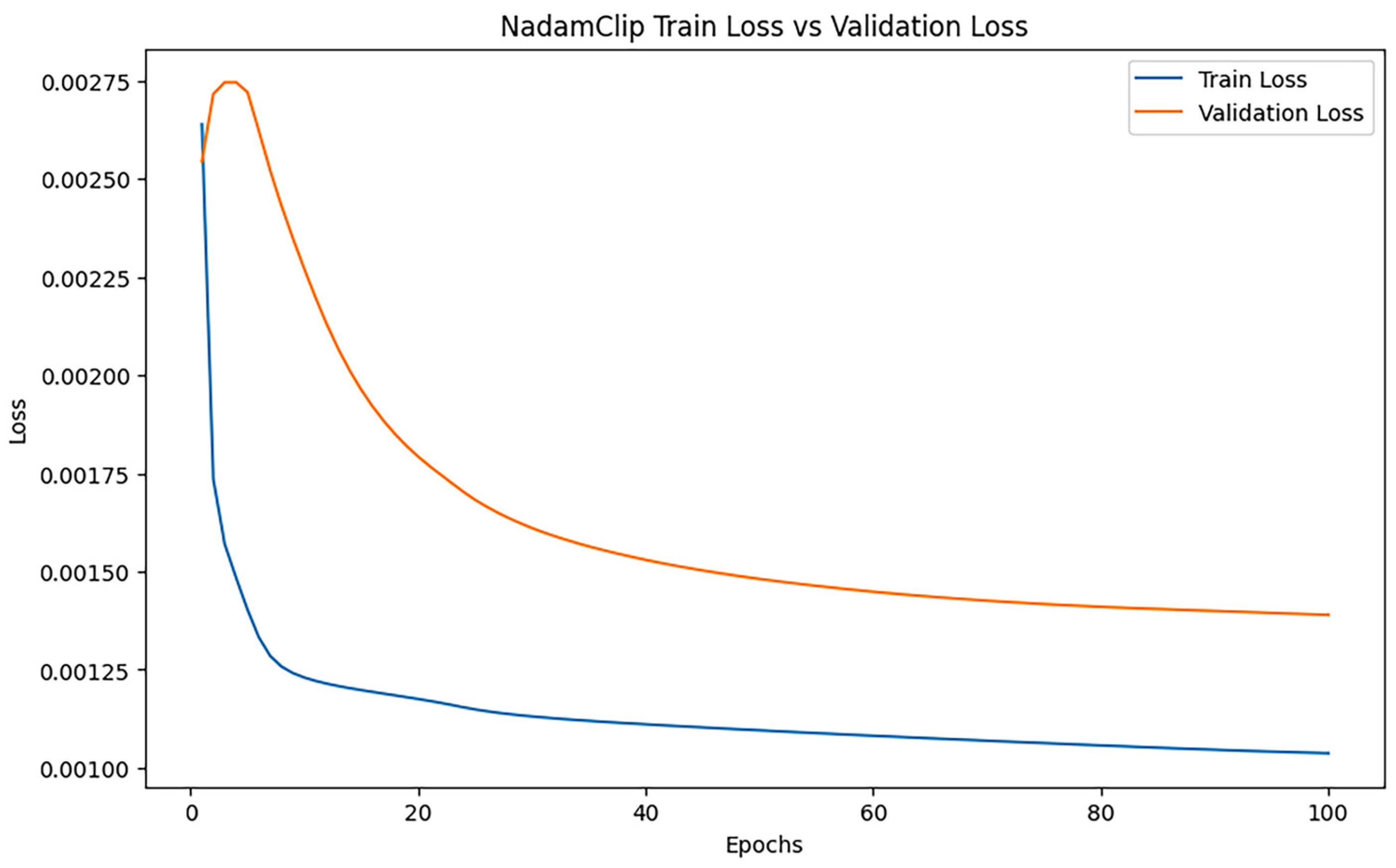
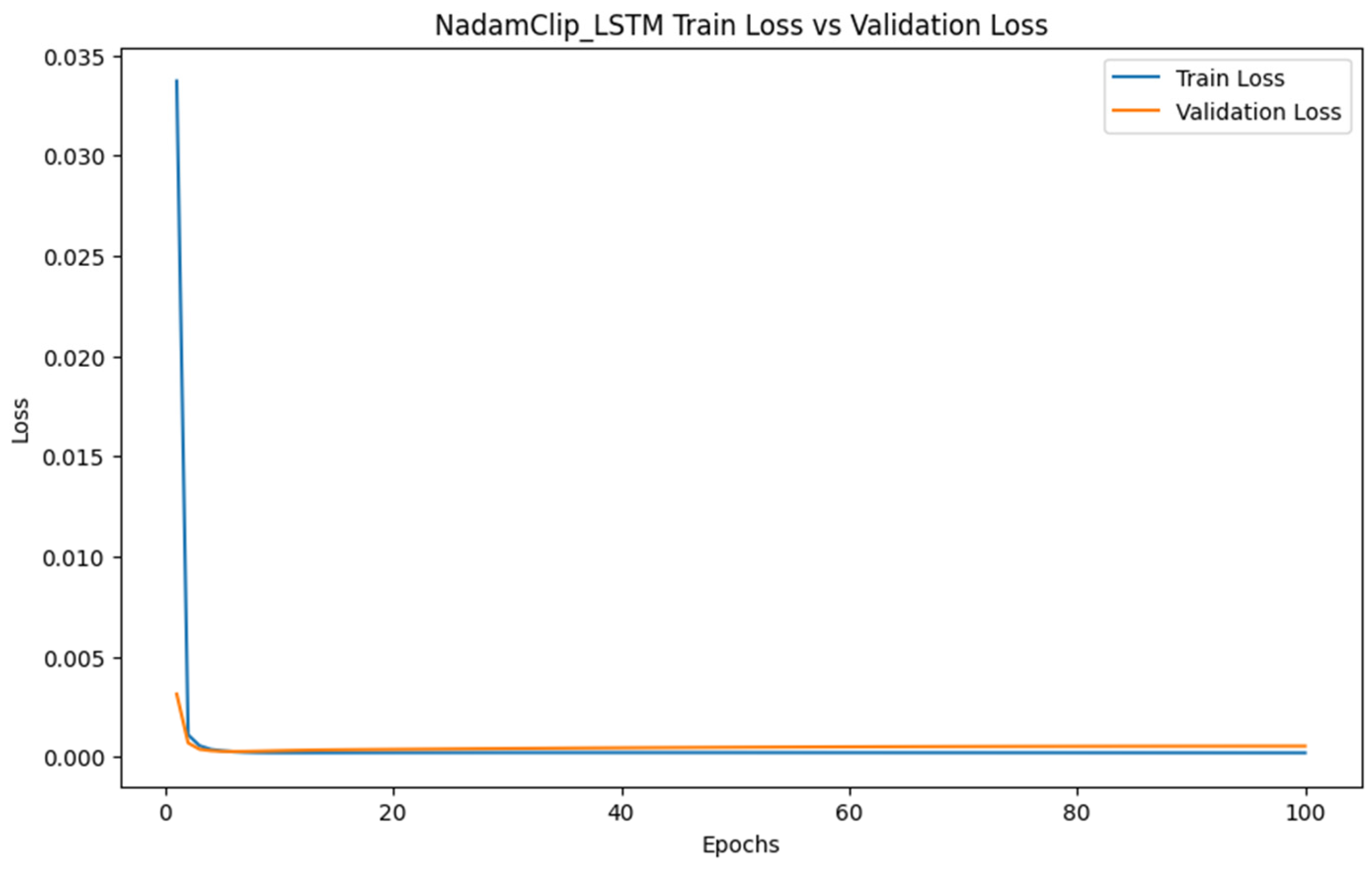
Training dynamics are visualized in Figure 3 and Figure 4, with loss trajectories and gradient norm evolution presented in the left and right panels, respectively. Figure 4 illustrates loss variations, where blue curves denote training losses and orange curves represent validation losses. Figure 5 displays gradient norm fluctuations, using blue to depict maximum unclipped gradients and orange to indicate clipped counterparts following threshold application.
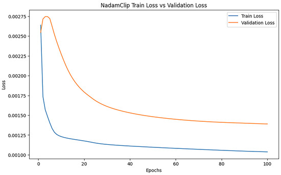
Figure 3.
NadamClip loss changes when clipping threshold is 100.

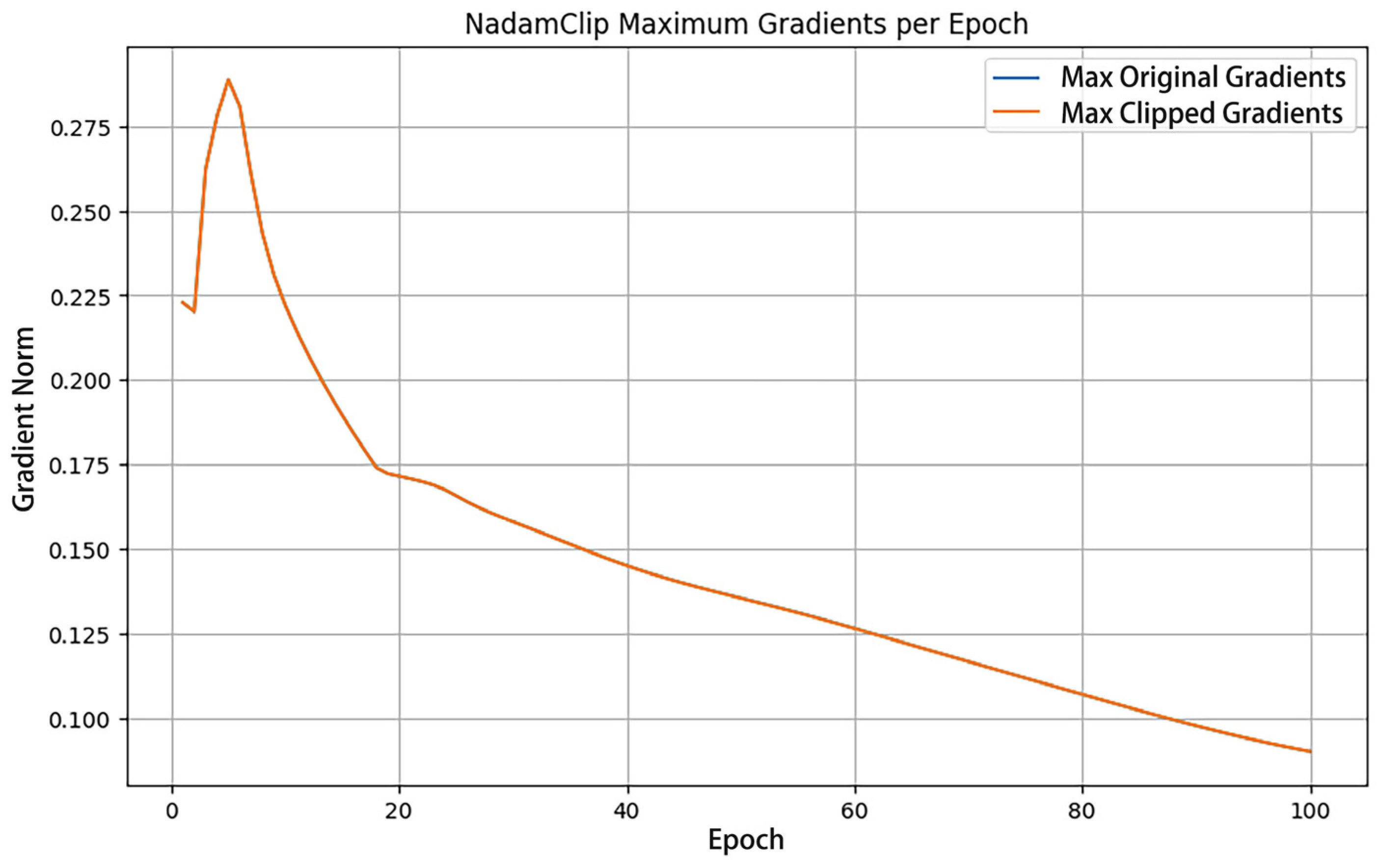
Figure 4.
Gradient norm change when clipping threshold is 100.
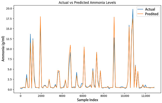
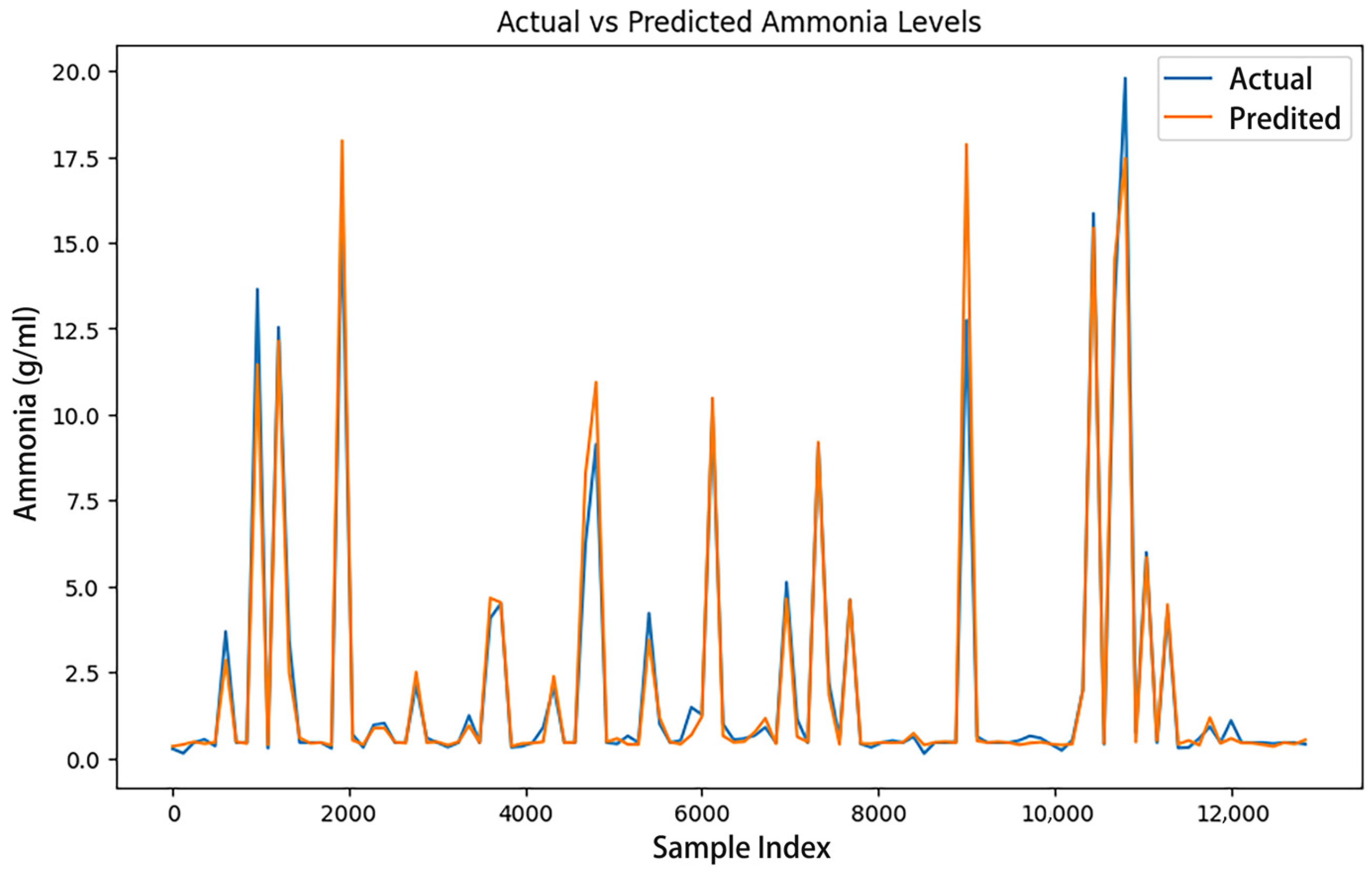
Figure 5.
NadamClip training model real value and predicted value comparison.
Figure 4 illustrates a gradient variation plot that compares the maximum original gradient with the clipped maximum gradient across each epoch. The figure illustrates that the maximum original gradient and the maximum clipped gradient coincide; thus, the gradient is not genuinely clipped. Concurrently, the value of the maximum gradient consistently rises or remains stable during the training process, signifying that the model’s optimization progressively approaches the ideal solution as training advances. This trend suggests that despite the rise in training losses, the model’s optimization remains effective, exhibiting stability and robust gradient updates.
Despite the gradient not being effectively clipped in this experiment, the model can nevertheless sustain a very stable updating process and gradually converge. However, even in the absence of explicit gradient explosion during training, gradient clipping remains a valuable technique. It serves as a preventive measure against occasional extreme gradient spikes, stabilizes parameter updates by limiting their magnitude, and enhances the overall robustness of the training process. Additionally, gradient clipping can have a regularization effect, guiding the model toward flatter minima and thereby improving generalization. Thus, it is not only a safeguard against instability but also a general strategy for promoting more reliable and effective training in complex models.
3.1.2. Gradient Clipping Range Experiment
This experiment aims to identify a gradient clipping range that optimally balances mitigating gradient explosion and preserving the model’s learning capacity. The original maximum gradient clipping value is 0.28. Based on this, a series of studies were conducted in which the gradient threshold was gradually reduced, with the adjustment calibrated to specific absolute values (e.g., 0.05). Initially, the gradient threshold was set to 0.25, a value chosen to effectively suppress gradient explosion without substantially diminishing the gradient. The corresponding model performance metrics, including RMSE, MAE, and R2, were then recorded.
- The gradient threshold is set to 0.25 as a large clipping value, meaning that during training, the gradient is clipped only if its absolute value exceeds 0.25. The model’s performance evaluation yielded the following metrics: MAE of 0.27233783261115885, RMSE of 0.6707561284835654, R2 of 0.9734625679547213, and gradient norm max of 0.2625596225261688.
- To optimize model performance, the gradient threshold was set to 0.2 to systematically evaluate the effects of controlled gradient norms on model training. This adjustment from 0.25 to 0.2 imposes stricter constraints on gradient update magnitudes. After completing 100 training epochs, the model’s evaluation showed an MAE of 0.2631191206486008, an RMSE of 0.662192962731887, an R2 of 0.9741358197337582, and a gradient norm max of 0.26188525557518005.
- The gradient threshold was configured at 0.15 to stabilize model training dynamics. Following rigorous training over 100 epochs, quantitative evaluation results included an MAE of 0.26790952024984593, an RMSE of 0.6687321135613868, an R2 of 0.9736224803807937, and a gradient norm max of 0.31249192357063293.
Experimental results demonstrate peak model performance at a gradient threshold of 0.2 (MAE = 0.2631, RMSE = 0.6622, R2 = 0.9741, maximum gradient norm = 0.2), significantly outperforming the 0.25 threshold configuration while maintaining moderate clipping intensity that achieves optimal equilibrium between training stability and model adaptability. Conversely, when reducing the threshold to 0.15, the MAE (0.2679) and RMSE (0.6687) show measurable increases with a corresponding R2 reduction (0.9736). Simultaneously, the maximum gradient norm rises to 0.3125, indicating that aggressive clipping not only restricts global gradient magnitudes but also triggers momentum accumulation effects in the optimizer, ultimately resulting in training oscillations and predictive performance degradation.
Consequently, the optimal threshold should be constrained within the 0.2–0.25 interval. Precision tuning experiments (0.21, 0.22, 0.23) reveal 0.2 as a critical balance point where gradient clipping effectively suppresses pathological oscillations while maintaining adequate parameter update flexibility to safeguard model expressiveness. This empirical evidence confirms the intrinsic trade-off in gradient truncation between constraint severity and learning potential, demonstrating that suboptimal thresholds (e.g., 0.15) destabilize the equilibrium state, whereas the 0.2–0.25 range achieves optimal regulatory effectiveness.
- The gradient threshold is established at 0.21 to enhance the stability of model training. Following iterative training for 100 epochs, performance assessment recorded an MAE of 0.26790952024984593, an RMSE of 0.6687321135613868, an R2 of 0.9736224803807937, and a gradient norm max of 0.31249192357063293.
- Set the gradient threshold to 0.22. After training iterations with epoch = 100, model evaluation produced an MAE of 0.2675364506810387, an RMSE of 0.6716723562013663, an R2 of 0.973390020165747, and a gradient norm max of 0.25483882427215576.
- Set the gradient threshold to 0.23. After training iterations with epoch = 100, performance metrics showed an MAE of 0.2649279389603518, an RMSE of 0.6644888459309692, an R2 of 0.9739561618993233, and a gradient norm max of 0.25819098949432373.
- Set the gradient threshold to 0.24. After training iterations with epoch = 100, evaluation results indicated an MAE of 0.2643528489751698, an RMSE of 0.6594540048675472, an R2 of 0.9743493357271562, and a gradient norm max of 0.2894490659236908.
All of the above training results are summarized in Table 6.
Table 6.
Results summarized.
The experimental results show that when the gradient threshold is 0.24, the model has the best performance (MAE = 0.2644, RMSE = 0.6595, R2 = 0.9743, maximum gradient norm = 0.2894), and the fitting error is minimal and the generalization ability is best while the gradient anomaly fluctuation is suppressed.
Figure 5 illustrates the comparison between the actual value and the forecasted value when the gradient threshold is set at 0.24.
Figure 5 shows that the anticipated value of the NadamClip optimizer closely aligns with the actual value, and the curve’s trajectory nearly coincides, indicating that the NadamClip optimizer effectively fits the data during training, resulting in more precise predictions. Throughout the entire data range, NadamClip’s predicted values exhibit reduced fluctuations and align consistently with the true values, demonstrating its superior performance in model fitting and predictive accuracy.
3.2. Comparison with Stochastic Gradient Descent Algorithm
This segment of the experiment examines the efficacy of the NadamClip method in comparison to conventional gradient descent algorithms. The prevalent algorithms comprise SGD, Adaptive Gradient Algorithm (AdaGrad) [25], Adaptive Delta Algorithm (AdaDelta) [26], Root Mean Square Propagation (RMSProp), Adam [27], and Nadam and Adam with Weight Decay (AdamW) [28]. The algorithm that combines the stochastic gradient descent algorithm and the gradient clipping technique is DPSGD [29], SGD with Clip, Clipped Reweighted AdaGrad with Delay (Clip-RadaGradD) [30], AdamW with Adaptive Gradient Clipping (AdamW_AGC) [31], and Clipped Gradient Adam (CGAdam) [32]. The aforementioned techniques possess extensive applicability and research significance in the optimization tasks of deep learning. Through the comparison of these algorithms, we can thoroughly examine the convergence characteristics, stability, and application of NadamClip in various training circumstances, thereby acquiring a deeper grasp of its attributes and potential.
3.2.1. SGD Algorithm
To evaluate the merits and drawbacks of the SGD and NadamClip optimization techniques, this experiment was conducted over 100 epochs, with all other parameters aligned with the hyperparameters of the NadamClip training model. The training results indicated an MAE of 0.7505734623731953, an RMSE of 1.1711739274031217, and an R2 of 0.9190955541603905. The loss changes (Figure 6) in the training process are shown as follows.
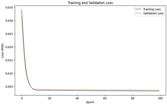
Figure 6.
SGD loss changes.
Figure 6 shows the absence of large fluctuations or increases in SGD losses, and the overall drop was minimal, suggesting a marginally diminished capacity for generalization. Consequently, NadamClip typically attains superior model performance more rapidly under same training settings.
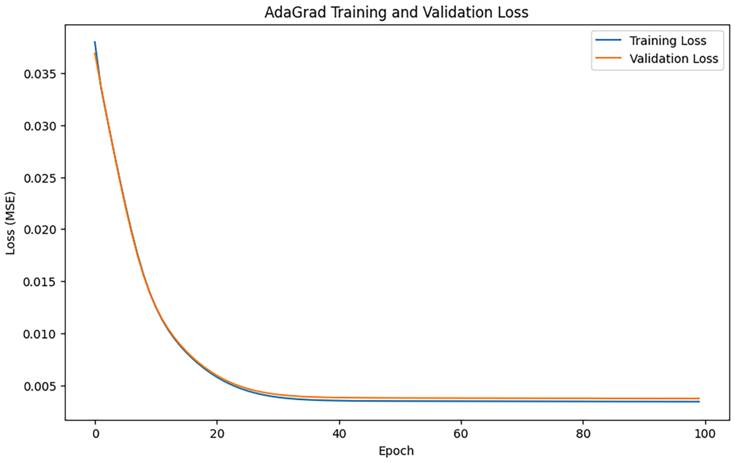
3.2.2. AdaGrad Algorithm
After training iterations with epoch = 100, the performance of the model was evaluated, and the training results indicated an MAE of 0.7821207436452577, 1.2046766764728003, and an R2 of 0.9144006236449291. Figure 7 shows the loss change of the AdaGrad algorithm.
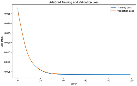
Figure 7.
AdaGrad loss changes.
Figure 7 illustrates that the training loss and the validation loss decline swiftly in the initial phase, signifying that the model effectively assimilates the data properties early on. Following approximately 20 iterations, the loss numbers stabilize, signifying that the model is nearing convergence. The training loss and validation loss curves are closely aligned, suggesting that the model did not experience substantial overfitting or underfitting issues during training.
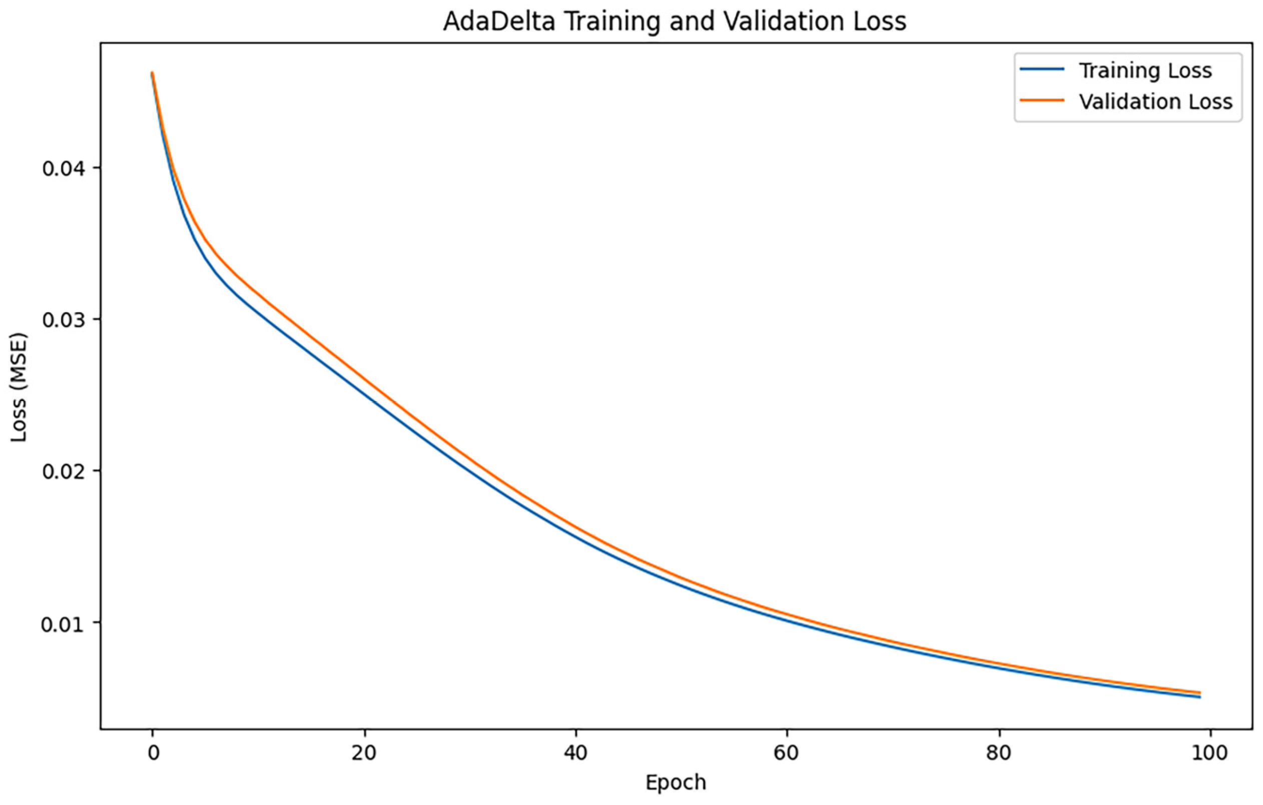
3.2.3. AdaDetla Algorithm
After training iterations with epoch = 100, the performance of the model was evaluated, and the training results indicated an MAE of 0.9210511548045627, 1.4274229448826565, and an R2 of 0.8798192407754606. Figure 8 shows the loss change of the AdamDetla algorithm.
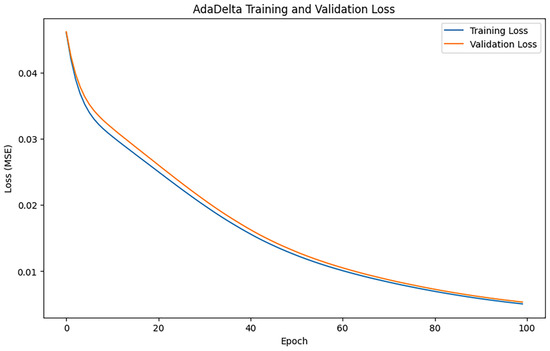
Figure 8.
AdaDetla loss changes.
Figure 8 illustrates a consistent decline in both training loss and validation loss, signifying that the model is persistently learning and optimizing. In comparison to other optimization techniques, AdaDelta exhibits a more gradual decline in loss, particularly during the later stages of iteration, where the decrease in loss values becomes significantly constrained.
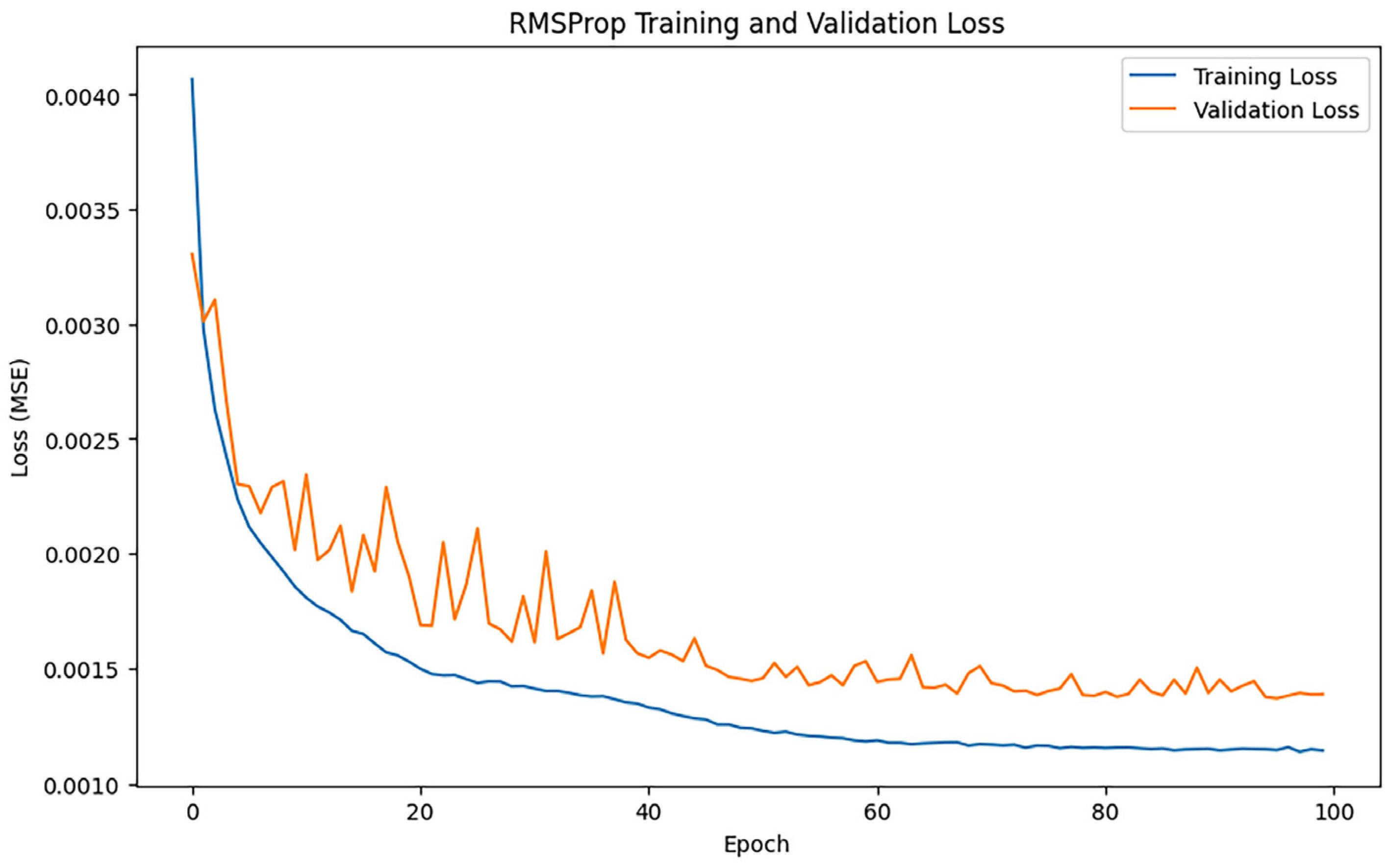
3.2.4. RMSProp Algorithm
After training iterations with epoch = 100, the performance of the model was evaluated, and the training results indicated an MAE of 0.3220789522245996, 0.6784517512974149, and an R2 of 0.9728501439025696. Figure 9 shows the loss change of the RMSProp algorithm.
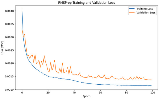
Figure 9.
RMSProp loss changes.
Figure 9 illustrates that both training loss and validation loss decline swiftly during the early phase, signifying the model’s effective acquisition of data properties at this time. The validation loss curve exhibits significant fluctuations, particularly during the mid and late stages of training, suggesting that the model’s performance on the validation data lacks stability, potentially influenced by noise or the constraints of the model’s generalization capacity.
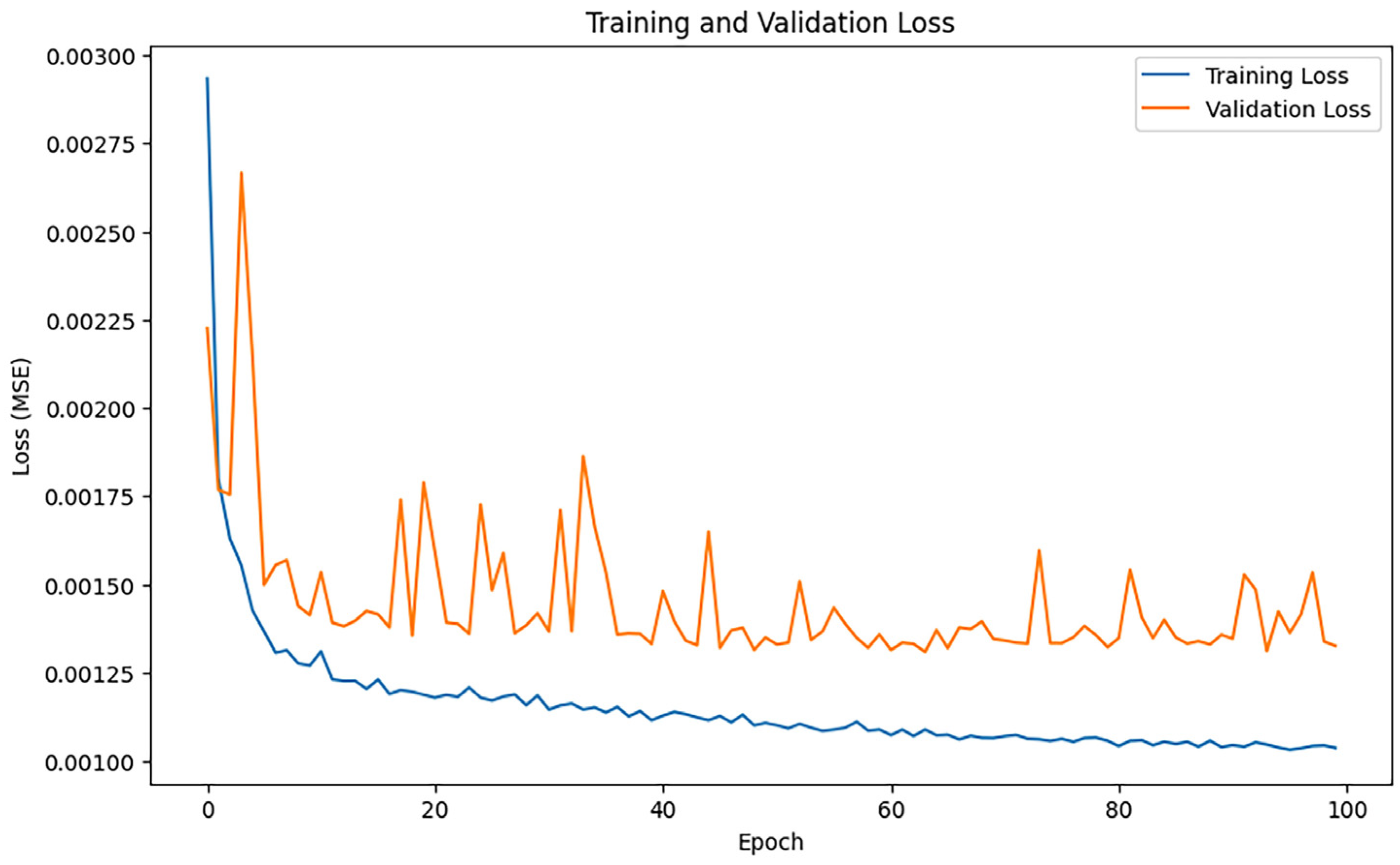
3.2.5. Adam Algorithm
Following 100 training epochs, the model’s performance was assessed, and the training results indicated an MAE of 0.26517207121185304, 0.6520466855995359, and an R2 of 0.974922341745961. Figure 10 shows the loss change of the Adam algorithm.

Figure 10.
Adam loss changes.
As illustrated in Figure 10, the training loss of Adam exhibited a rapid decline, with a pronounced reduction during the initial phase; however, in the subsequent phase, the training loss stabilized, and the rate of drop diminished progressively. The validity loss diminishes swiftly during the initial period but persists in fluctuating.
3.2.6. AdamW Algorithm
After training iterations with epoch = 100, the performance of the model was evaluated, and the training results indicated an MAE of 0.28577964900318875, 0.6770786502305564, and an R2 of 0.9729599284872327. Figure 11 shows the loss change of the AdamW algorithm.
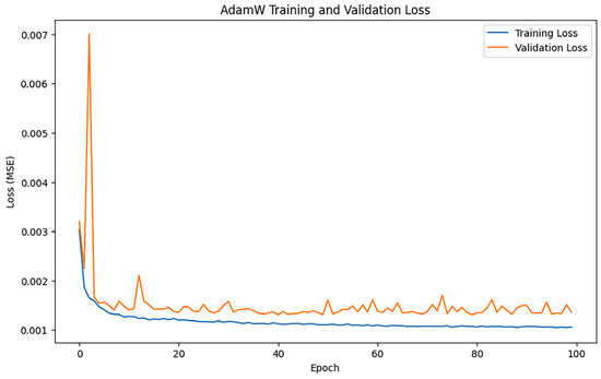
Figure 11.
AdamW loss changes.
Figure 11 illustrates the trends of training loss and validation loss for the AdamW algorithm throughout the training process. The training loss exhibits a swift decline and smooth convergence, signifying that AdamW effectively optimizes the model’s parameters.
3.2.7. Nadam Algorithm
Following 100 training epochs, the model’s performance was assessed, and the training results indicated an MAE of 0.2684995375430839, 0.6678549834047971, and an R2 of 0.9736916301768074. Figure 12 shows the loss change of the Nadam algorithm.
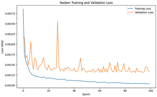
Figure 12.
Nadam loss changes.
As shown in Figure 12, the training loss of Nadam decreases faster in the initial phase, but the loss curve fluctuates significantly as the training progresses.
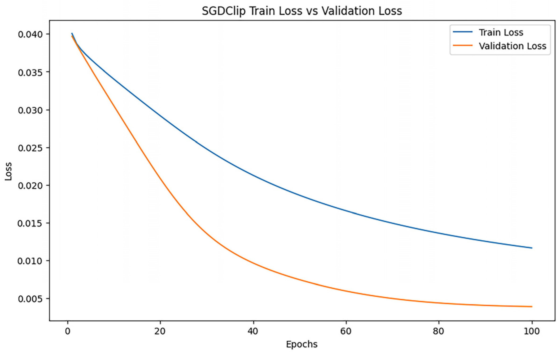
3.2.8. SGD with U-Clip Algorithm
After training iterations with epoch = 100, the performance of the model was evaluated, and the training results indicated an MAE of 0.8108290857223689, 1.2470619331350854, and an R2 of 0.9082712149511512. Figure 13 shows the loss change of SGD with the U-Clip algorithm.
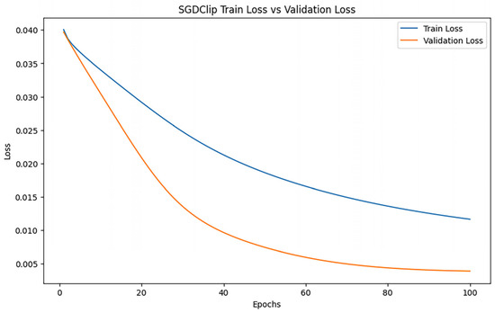
Figure 13.
SGD with U-Clip loss changes.
Figure 13 shows that the model can fit well on both training data and validation data, and the training process is smooth. However, with the deepening of training, the performance of the model did not continue to improve significantly, and the verification loss remained at a relatively stable low level, indicating that the training process was close to convergence but could not be further optimized.
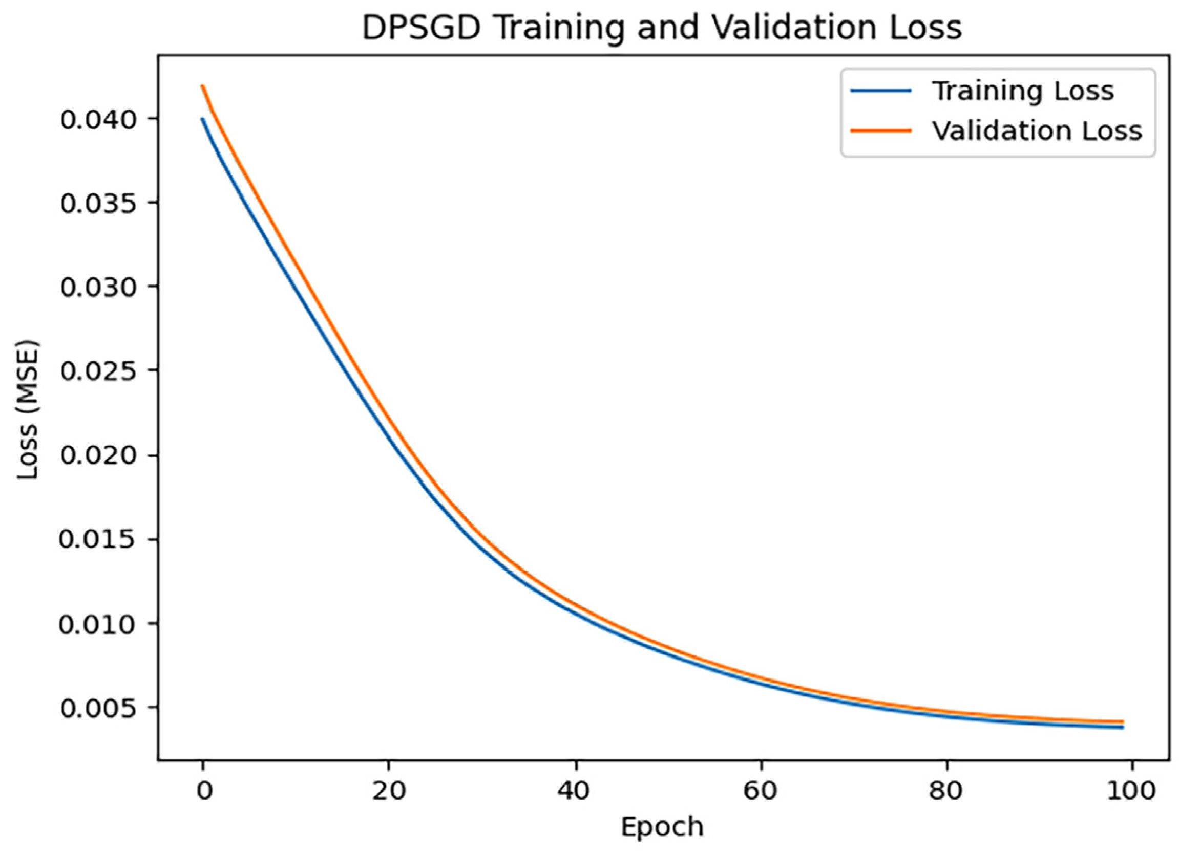
3.2.9. DPSGD
After training iterations with epoch = 100, the performance of the model was evaluated, and the training results indicated an MAE of 1.2594584818344572, 0.8108990966161156, and an R2 of 0.9064384716813607. Figure 14 shows the loss change of the DPSGD algorithm.
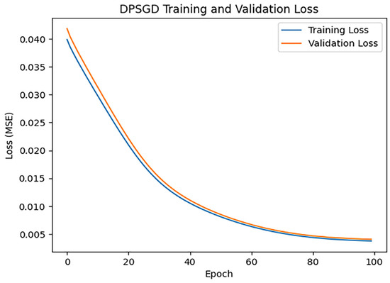
Figure 14.
DPSGD loss changes.
Figure 14 illustrates a more gradual decline in the loss. This may be attributable to the introduction of gradient clipping and noise in the gradient update by DPSGD, which may constrain the model’s capacity for rapid optimization while safeguarding privacy.
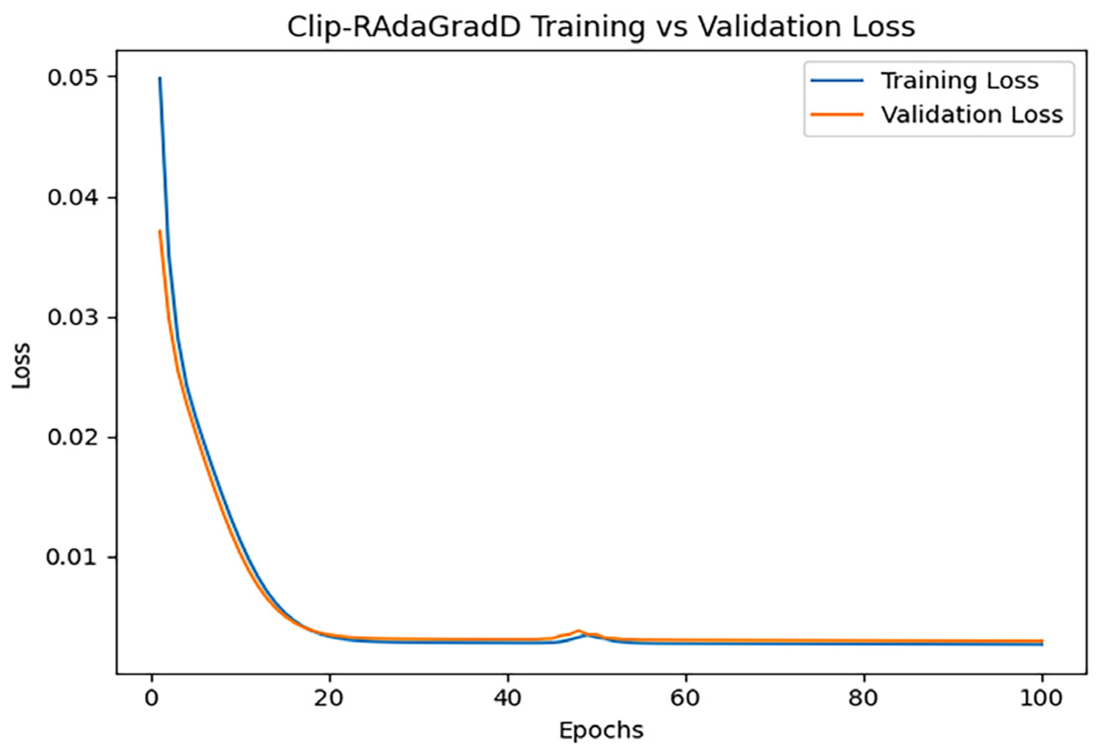
3.2.10. Clip-RAdaGradD
After training iterations with epoch = 100, the performance of the model was evaluated, and the training results indicated an MAE of 0.6614861471415543, 1.07210966116476, and an R2 of 0.9322033842309119. Figure 15 shows the loss change of the Clip-RAdaGradD algorithm.
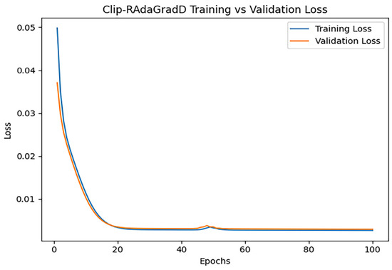
Figure 15.
Clip-RAdaGradD loss changes.
Figure 15 illustrates a rapid decline in both training loss and validation loss during the initial phase, signifying the model’s efficient learning of data features. Following approximately 20 iterations, the loss numbers settle, indicating that the model has effectively converged.
3.2.11. CGAdam
After training iterations with epoch = 100, the performance of the model was evaluated, and the training results indicated an MAE of 0.26186467218314385, 0.6581578685817608, and an R2 of 0.9744500677986624. Figure 16 shows the loss change of the CGAdam algorithm.
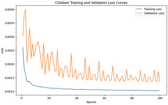
Figure 16.
CGAdam loss changes.
As can be seen from Figure 16, the training loss decreases rapidly and flattens out in the early stage, indicating that CGAdam is able to optimize the model quickly and converge stably. However, the curve of the validation loss shows obvious fluctuations, especially in the early and middle phases, showing some instability despite the overall trend of slow decrease.
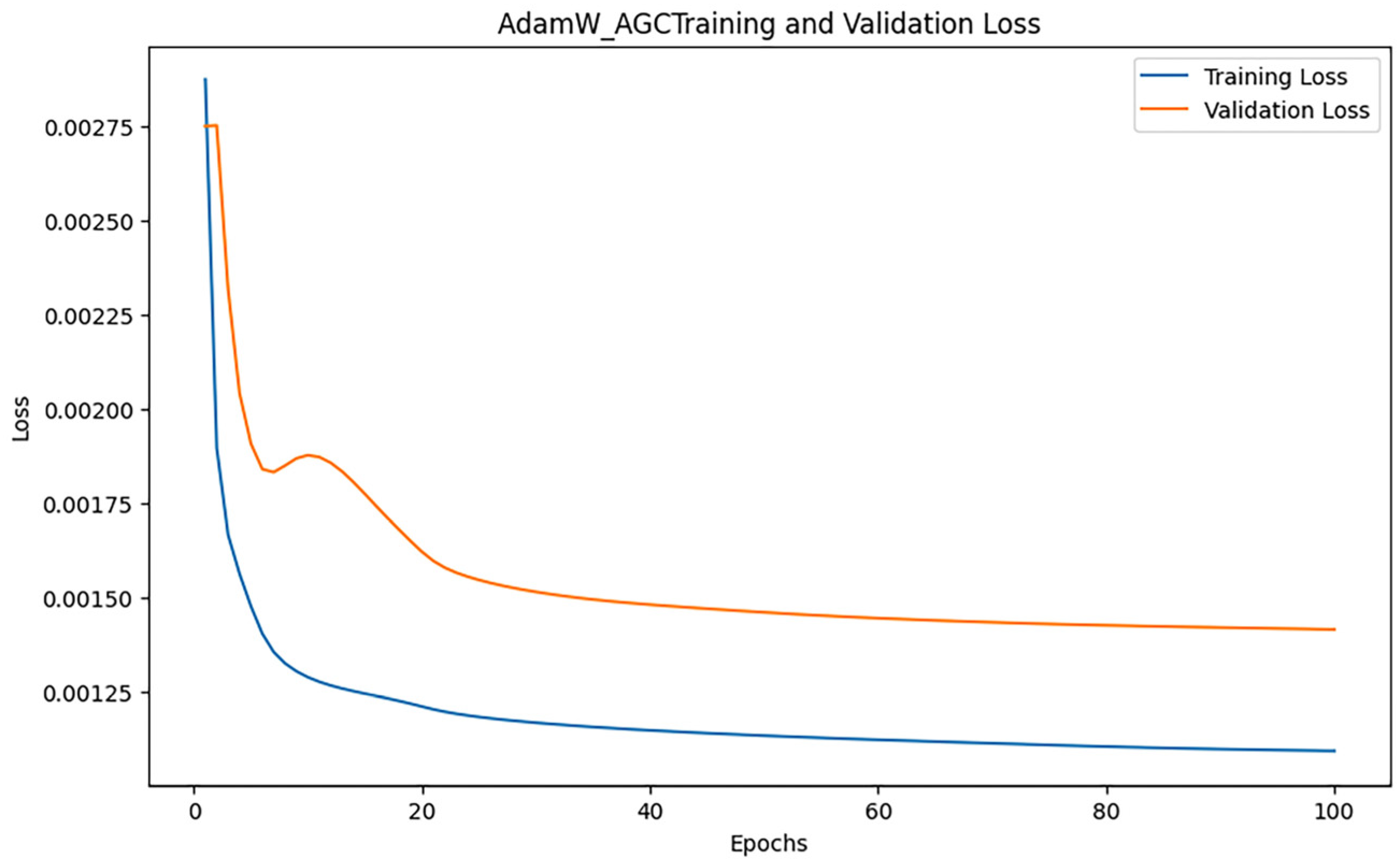
3.2.12. AdamW_AGC
After training iterations with epoch = 100, the performance of the model was evaluated, and the training results indicated an MAE of 0.27305611051047424, 0.6829421034527225, and an R2 of 0.9724895704203821. Figure 17 shows the loss change of the AdamW_AGC algorithm.
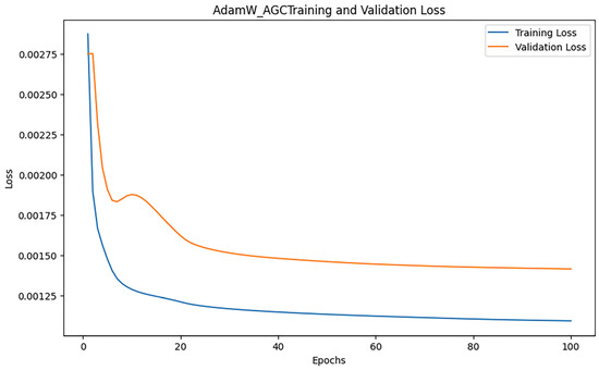
Figure 17.
AdamW_AGC loss changes.
Figure 17 illustrates the trend of training loss and validation loss of the AdamW_AGC algorithm according to the epoch throughout the training process. The training loss exhibits a rapid decline in the initial phase and stabilizes in the later phase, indicating the swift convergence capability of AdamW_AGC.
3.3. Comparison of Measurement Results
To comprehensively evaluate the prediction accuracy of different optimization algorithms, the evaluation results of the aforementioned 13 optimization algorithms have been summarized, as shown in Table 7. Comparing the performance of these algorithms in terms of RMSE, MAE, and R2 can provide a deeper understanding of the adaptability and performance differences of these algorithms in different tasks and provide a more scientific basis for model selection.
Table 7.
Summary of 13 algorithmic measurements.
Among the evaluated algorithms, CGAdam, NadamClip, and Adam demonstrate superior performance. Within this top tier, CGAdam achieves the lowest RMSE (0.2619), marginally outperforming both NadamClip (0.2644) and Adam (0.2652), establishing it as the overall leader in this metric. Its MAE (0.6582) also ranks competitively, second only to Adam’s optimal value (0.6520), while its R2 (0.9745) indicates an effective balance between precision and model fit. Adam distinguishes itself with the best MAE (0.6520) and the highest R2 (0.9749), reflecting exceptional stability. Although NadamClip slightly trails CGAdam and Adam across metrics, it remains highly robust, with near-optimal performance in all three criteria.
In contrast, traditional or privacy-enhanced optimizers—including SGD, AdaDelta, SGD with U-Clip, and DPSGD—exhibit markedly inferior results. DPSGD yields the highest RMSE (1.2594), a substantially elevated MAE (0.8108), and the lowest R2 (0.9064), demonstrating that its privacy guarantees sacrificed substantial model accuracy. AdaDelta performs particularly poorly in MAE (1.4274), coupled with a high RMSE (0.9211), indicating fundamentally inadequate fitting capability for this task.
Mid-tier performers comprise RMSProp, Nadam, AdamW, and AdamW_AGC. RMSProp achieves an RMSE of 0.3221, moderately higher than Adam-type optimizers yet still surpassing traditional SGD, while its R2 (0.9729) confirms strong fitting competence. AdamW_AGC delivers balance though unexceptional metrics across all criteria, outperforming algorithms like AdaGrad and Clip-RAdaGradD in stability despite falling short of Adam and CGAdam.
CGAdam, NadamClip, and Adam emerge as the most effective optimizers for this regression task, making them ideal for modeling scenarios strictly requiring high precision. Conversely, traditional and privacy-preserving algorithms incur significant accuracy trade-offs.
3.4. Comparison of Loss Results
This section contrasts NadamClip, SGD, AdaGrad, AdaDelta, RMSProp, Adam, Nadam, AdamW, DPSGD, and SGD with U-Clip, alongside the loss trends of Radagadd, CGAdam, and AdamW_AGC algorithms throughout training, to assess their efficacy under varying training settings.
3.4.1. Comparison of Training Loss
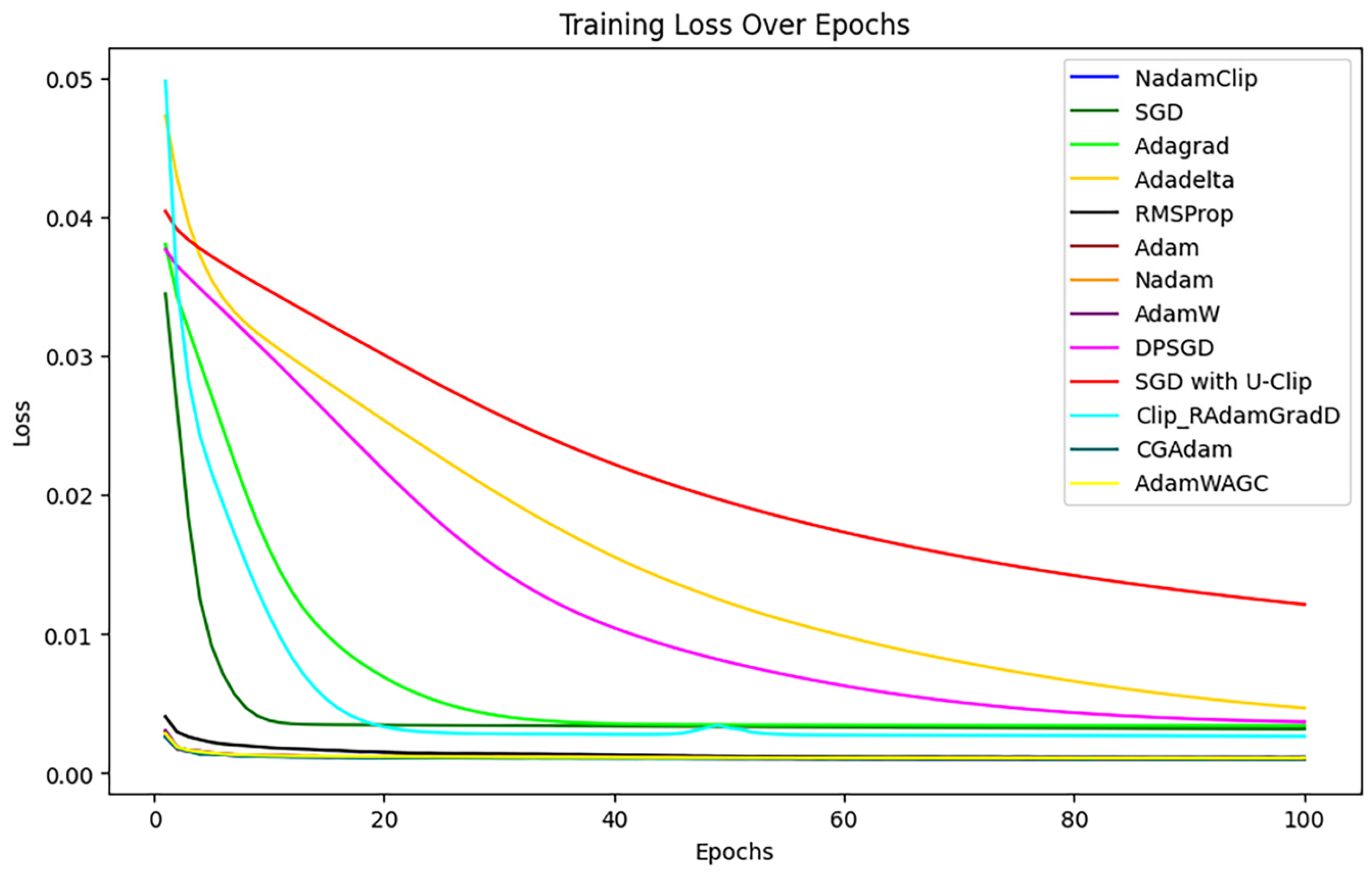
First, the training loss of each algorithm is visualized with the change of time or number of iterations, as shown in Figure 18 below.
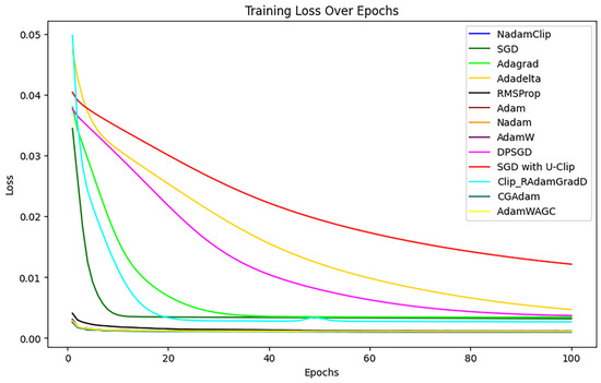
Figure 18.
Training loss comparison.
The experiment demonstrated that the loss of SGD with U-Clip (red), AdaDelta (yellow), and DPSGD (pink) diminished gradually throughout the initial phase of training, particularly SGD with U-Clip, which exhibited a mild loss curve and the least reduction.
For a clearer comparison, the overlapping loss curves were magnified, as shown in Figure A2 in Appendix B. It was observed that the RMSProp loss diminishes at a markedly slower rate than the other algorithms, resulting in a final loss that exceeds that of the alternatives. Hence, RMSProp was excluded from further comparisons.
The comparison then continues with other algorithms, as show in Figure A2 in Appendix B. The loss curves of Nadam, Adam, CGAdam, and AdamW exhibit a certain degree of oscillation throughout the training phase. The oscillation phenomenon typically indicates the model’s sensitivity to gradient variations during optimization, perhaps resulting in recurrent adjustments in specific areas and an inability to converge stably to the global optimal solution. NadamClip and AdamW_AGC exhibit relative stability, while Nadam and Adam have been excluded to facilitate a clearer comparison of the performance between NadamClip, AdamW_AGC, CGAdam, and AdamW, as illustrated in Figure 19.
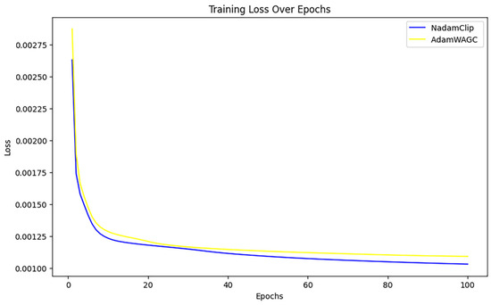
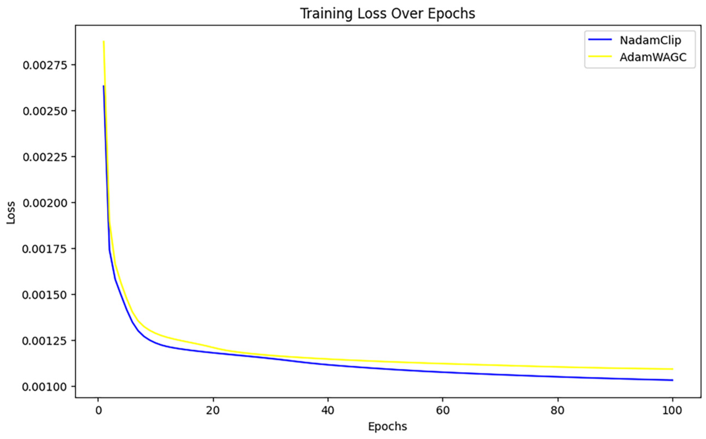
Figure 19.
Comparison of training losses for NadamClip, AdamW_AGC Tran.
Figure 19 illustrates that the loss curves of both optimization techniques decline swiftly in the initial phase, indicating a more rapid convergence rate. As training progresses, the curves of both models increasingly stabilize, signifying improved convergence in the later stages of training.
The training loss of NadamClip is marginally smaller than that of AdamW_AGC during the training process, particularly in the later stages, where the disparity becomes more pronounced. This indicates that NadamClip has superior optimization efficiency and final loss management, demonstrating an enhanced capacity to adapt to training data and identify optimal solutions more effectively. In conclusion, while both exhibit commendable optimization performance, NadamClip demonstrates less loss in the latter stages of training and marginally superior convergence compared to AdamW_AGC.
Therefore, in this comparison, NadamClip outperforms and enhances the model’s stability during training.
3.4.2. Verification Loss Comparison
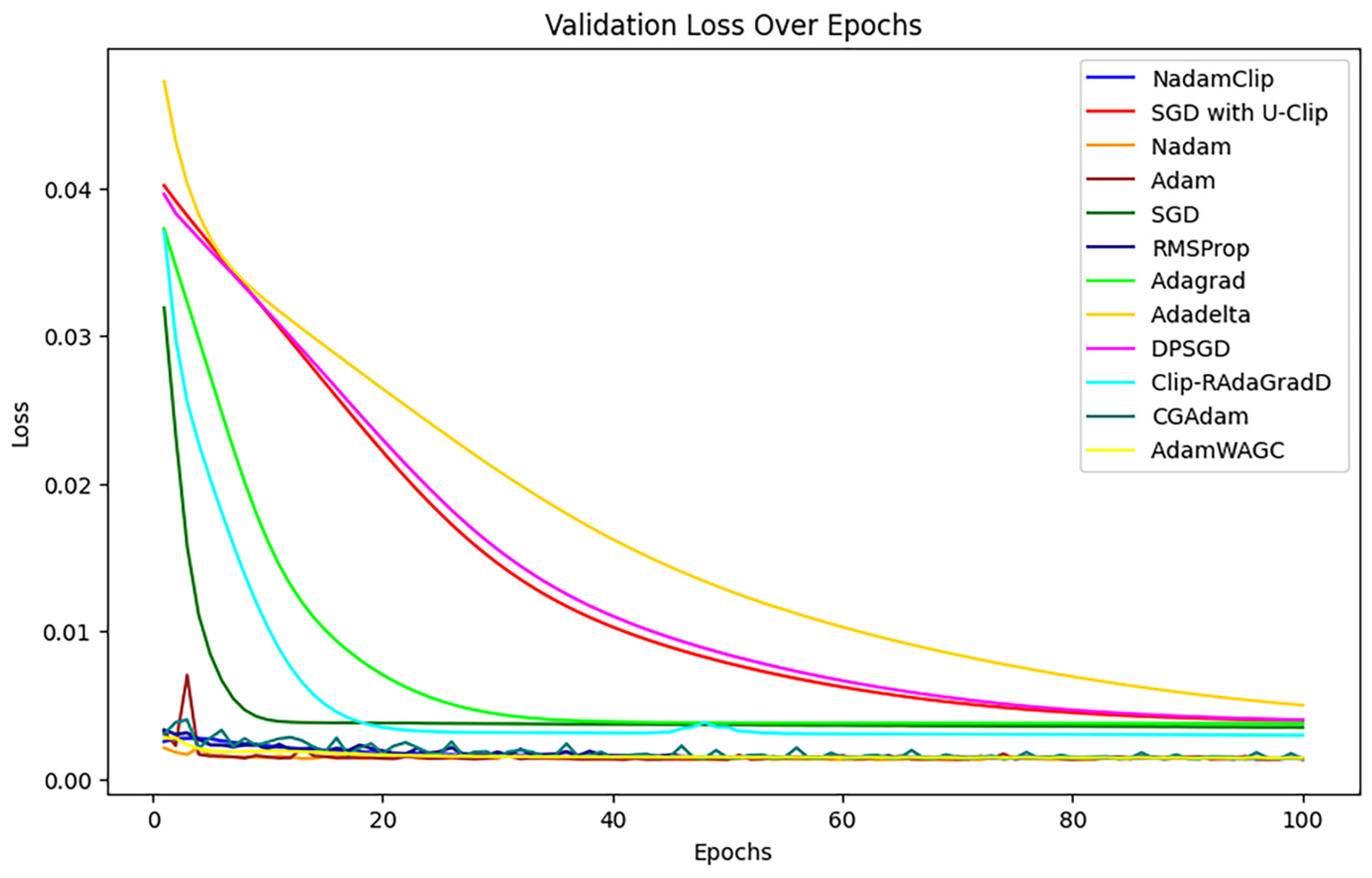
Subsequent comparisons were made to verify the change in loss, as shown in Figure 20.
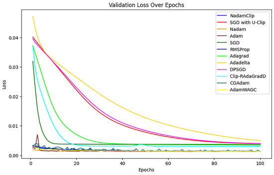
Figure 20.
Comparison of validation losses.
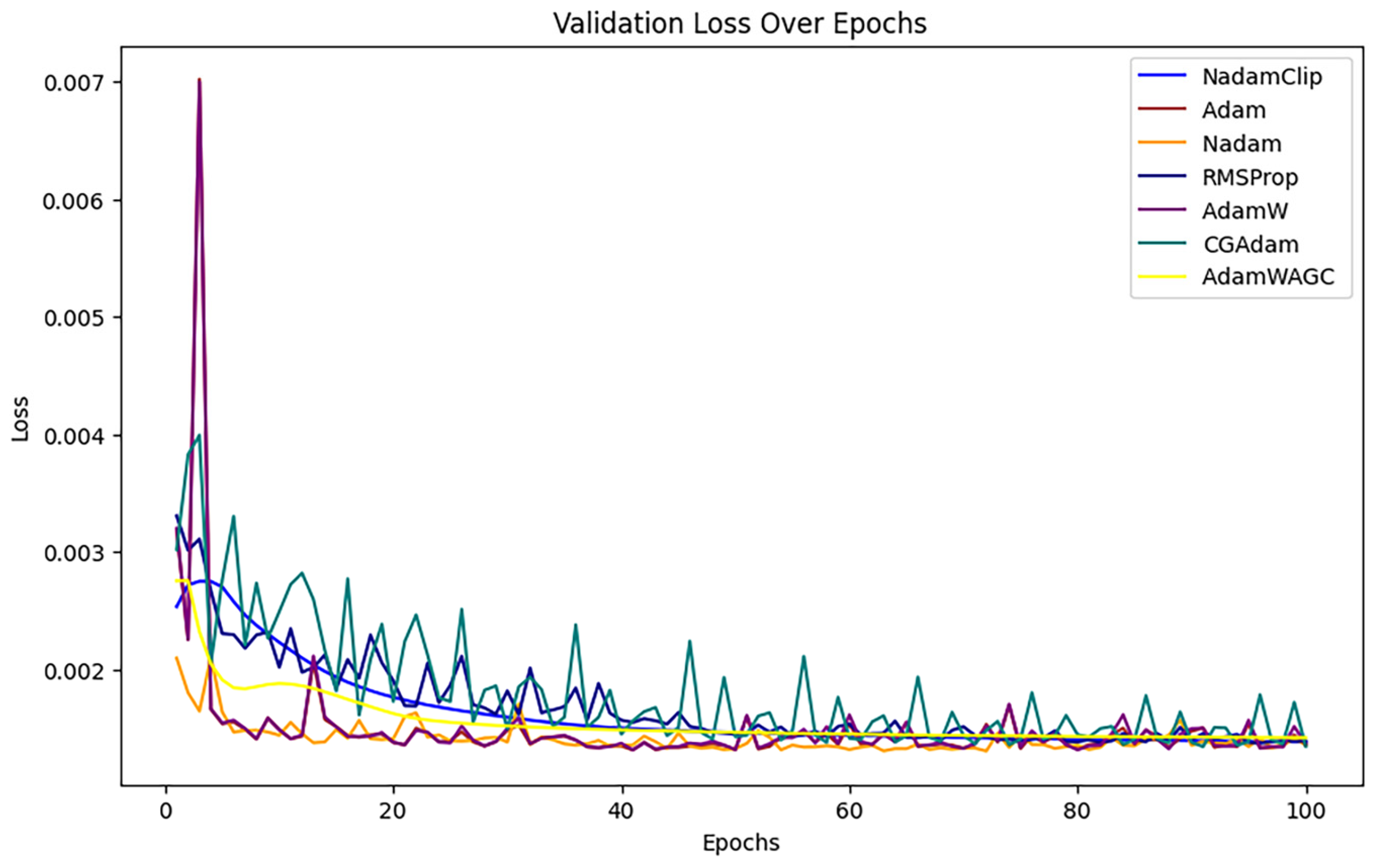
NadamClip, RMSProp, Adam, Nadam, AdamW, CGAdam, and AdamWAG exhibit better results relative to SGD with U-Clip, AdaDelta, DPSGD, AdaGrad, Clip_RAdamGradD, and SGD, indicating ongoing overlap in their efficacy. Therefore, we magnified them to continue the comparison, referring to Figure A3 in Appendix B.
Upon magnification, the loss curves of Nadam, Adam, CGAdam, and AdamW exhibit discernible oscillations during the training phase. Their exclusion facilitates a more direct comparative analysis between NadamClip and AdamW_AGC.
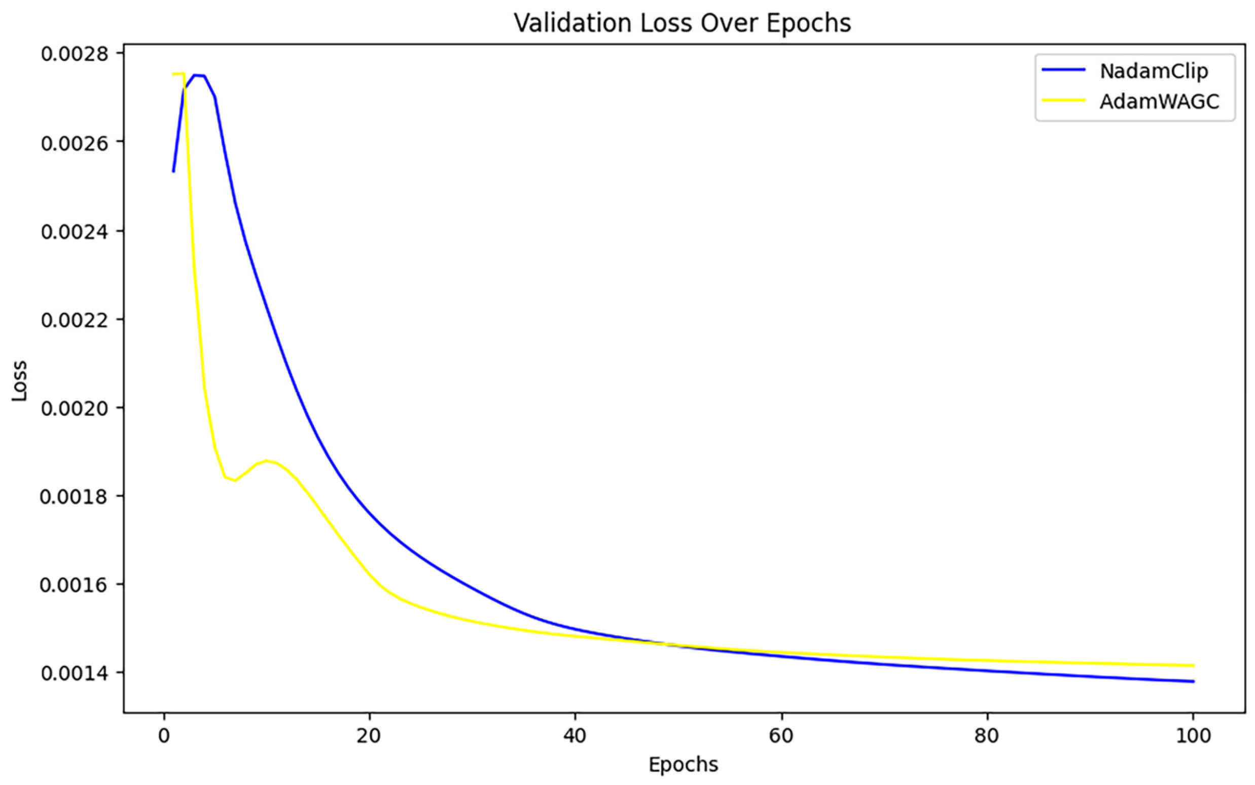
Figure 21 compares the final validation loss between the two algorithms. It reveals that the final validation loss of AdamW_AGC and NadamClip at the conclusion of training is nearly identical, and NadamClip is slightly better than AdamW_AGC.
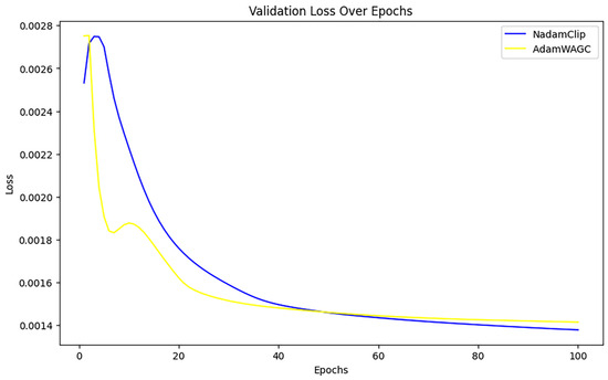
Figure 21.
Comparison of validation losses for NadamClip, AdamW_AGC.
3.5. Comparison of Computing Resource Consumption
During the training of the algorithms, the training time, Current Memory Usage, and Peak Memory Usage of each algorithm were recorded, as shown in Table 8.
Table 8.
Summary of computational overhead results for 13 algorithms.
Experimental evaluations reveal significant differences in computational efficiency and resource requirements among the different optimization algorithms. Clip-RadaGrad exhibits the optimal training efficiency (488.3 s) and maintains a moderate memory footprint, highlighting its strength in time-sensitive scenarios. In contrast, DPSGD has the highest computational overhead (15,721.7 s) and significantly higher peak memory consumption (42.5 MB) than the other algorithms, indicating its resource-intensive nature. Among the commonly used methods, AdamW is efficient in terms of training time (642.7 s) and memory usage (12.2 MB peak). NadamClip has a longer training time (12,114.7 s), but its memory consumption is the lowest (11.0 MB peak), demonstrating its excellent memory efficiency. AdamW_AGC has a moderate training time (7856.5 s) but a higher memory requirement (11.0 MB peak). AdamW_AGC has a moderate training time (7856.5 s) but a high memory requirement (32.0 MB peak). Traditional methods, such as SGD, AdaGrad, and RMSProp, are moderately efficient, but AdaGrad’s peak memory (17.3 MB) is particularly impressive, while SGD with U-Clip achieves the lowest memory footprint (5.0 MB peak) at the expense of a significantly longer training time (10,245.2 s) (7.6 MB peak memory, 12,567.7 s training time). In summary, Clip-RadaGrad and AdamW lead in overall efficiency, while the resource requirements of DPSGD and AdamW_AGC limit their applicability; NadamClip and SGD with U-Clip are the preferred choices for memory-constrained environments. Algorithm selection requires a trade-off between computational speed and resource consumption based on task requirements.
3.6. Applications in Other Datasets
To demonstrate the broad applicability of the NadamClip optimization technique, a Google stock prediction dataset from Kaggle was utilized. The dataset has 14 columns and 1257 rows, with the adjusted high price, adjusted low price, adjusted open price, and adjusted trading volume designated as input characteristics, while the adjusted close price is identified as the goal variable for prediction. The NadamClip optimization approach was employed to train the LSTM model while maintaining consistent hyperparameter settings with the ammonia prediction trials, hence further substantiating the usefulness and resilience of NadamClip for complicated time series tasks across several domains.
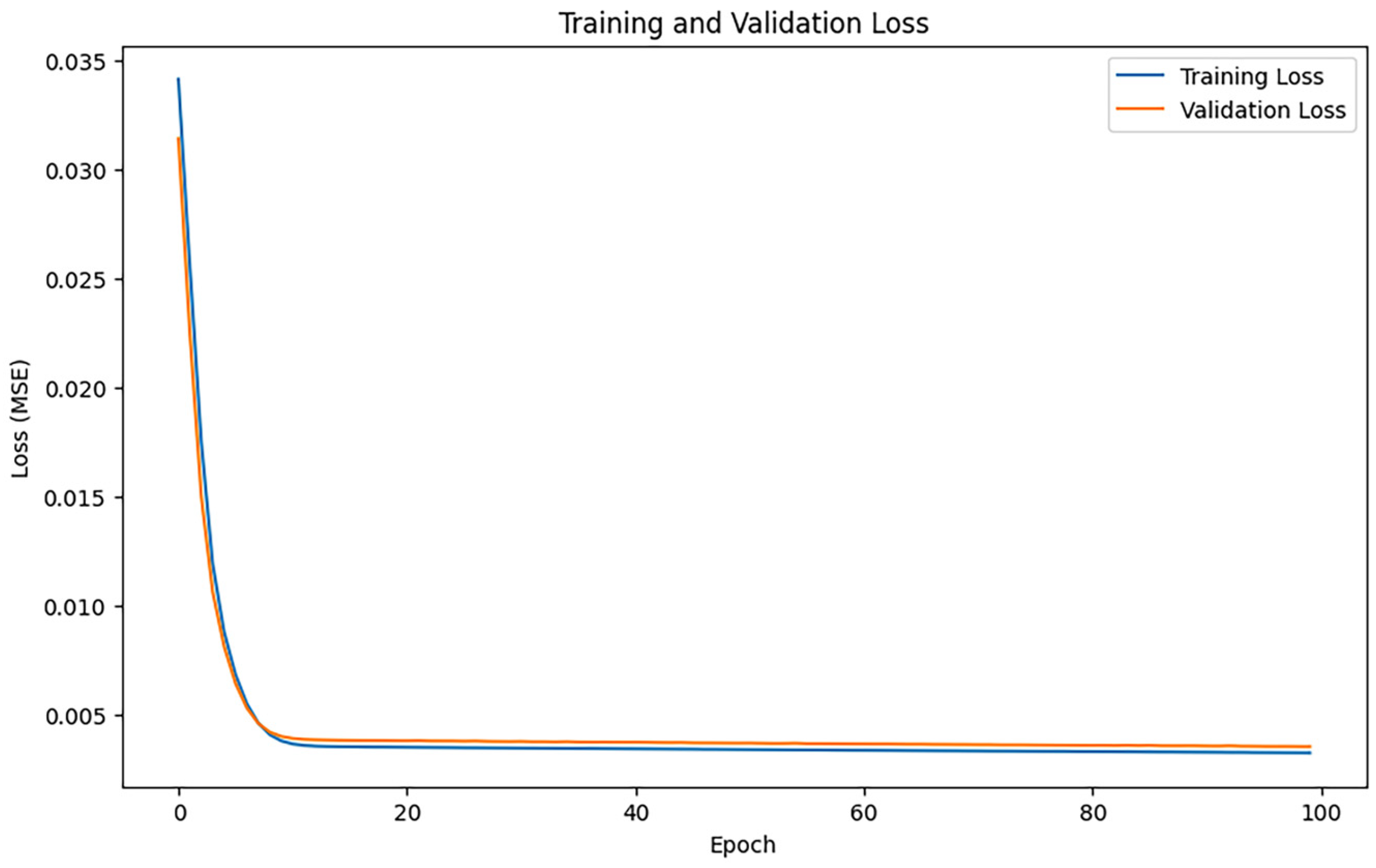
The training yielded a Mean Absolute Error (MAE) of 24.85 and a Root Mean Square Error (RMSE) of 35.72, which corresponded to 2.04% and 2.94% of the mean of the values of the target variable and 1.34% and 1.93% of the extreme deviation of the values of the target variable, respectively. The error proportions are minimal, suggesting that the model’s prediction error is nearly insignificant compared to the scale of the target variable. Furthermore, the model possesses an R2 value of 0.9903, signifying that it accounts for approximately 99% of the variations in the target variable. Collectively, these measurements indicate that the model’s predictive accuracy is exceptionally high and effectively captures stock price trends, offering dependable support for financial time series forecasting endeavors. Figure 22 shows the loss change of the dataset.
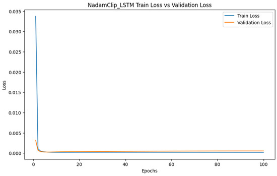
Figure 22.
Stock prediction loss changes.
As shown in Figure 22, both the training loss and validation loss decreased rapidly in the initial phase and subsequently converged to a stable state. The nearly overlapping curves indicate that the model possesses strong generalization capabilities without significant overfitting or underfitting. The smoothness and rapid convergence of the curves demonstrate the stability and efficiency of the NadamClip optimization process, which facilitates effective learning of the relationship between input features and the target variable.
Comprehensive experimental results indicate that NadamClip consistently delivers strong performance across various time series forecasting tasks, exhibiting high accuracy, stability, and generalization ability. Empirical validation on financial time series further confirms the robustness and adaptability of this optimization approach across diverse data and application scenarios.
4. Discussion
In the experimental comparisons in this study, there are differences in the performance of different optimization algorithms in the time series prediction task. Overall, CGAdam, NadamClip, and Adam demonstrate relatively strong performance on several evaluation metrics, achieving high regression accuracy. CGAdam shows a slight advantage on RMSE, while Adam performs slightly better on MAE and R2 metrics. While NadamClip slightly underperforms CGAdam and Adam on individual metrics, it performs very close to both methods on all three core evaluation criteria.
NadamClip’s performance is evident not only in error metrics but also in training stability. During training, this method exhibited smaller oscillation amplitudes and faster convergence compared to other optimizers, particularly in the later stages, where its loss curve became notably smoother. This stability stems from its enhanced mechanism, which integrates an error-compensated gradient clipping strategy on top of the Nadam optimizer. Specifically, after each gradient clipping operation, the algorithm temporarily stores the truncated gradient components and incrementally reintegrates them in subsequent training steps. This effectively mitigates the bias introduced by gradient clipping, thereby enhancing the robustness of the training process and optimizing accuracy. Consequently, it achieves a well-balanced trade-off between prediction accuracy and training stability.
To validate the method’s general applicability, this study employed two distinct types of time series datasets: ammonia nitrogen concentration prediction data from environmental monitoring and stock price time series data from the financial domain. NadamClip demonstrated stable and accurate optimization capabilities in both tasks, indicating its strong adaptability to diverse data structures and application scenarios. This cross-domain consistency further supports the viability of NadamClip as a general-purpose optimizer and suggests its promising generalization potential.
In summary, NadamClip achieves relatively stable convergence, exhibits favorable training dynamics, and holds potential advantages for long-term optimization and generalization. Therefore, within the context of this comparative experiment, NadamClip demonstrated superior overall performance, effectively balancing stability and memory efficiency, making it a suitable choice for training complex models.
5. Conclusions
This study proposes an enhanced adaptive optimizer, NadamClip, designed to address the challenges of stability and accuracy in predicting key parameters within complex bio-process environments typical of manufacturing systems. The method systematically embeds a gradient clipping mechanism within the Nadam optimizer for the first time, achieving deep integration of gradient truncation with momentum estimation and adaptive learning rates. Unlike traditional approaches that treat gradient clipping as an external add-on strategy, NadamClip fundamentally breaks the paradigm of “external control” at the algorithmic architecture level. This enables automatic modulation of the parameter update magnitude during anomalous gradient disturbances, effectively mitigating gradient explosion and enhancing training stability.
Through empirical studies on time series prediction tasks involving non-stationary and dynamic environmental parameters, NadamClip demonstrated high adaptability to network convergence characteristics across multiple training phases. It not only improved model robustness and generalization capabilities but also significantly optimized convergence efficiency and final prediction accuracy. Compared to existing optimizers and their variants, NadamClip achieved a relatively good balance between stability and convergence speed, providing a novel conceptual framework and technical approach for optimizer design in time series forecasting.
Validation on diverse datasets, including representative biological processes and financial modeling, further demonstrates that this optimization method is not only suitable for environmental process control but also readily applicable to a broad range of manufacturing scenarios. These encompass industrial process modeling, process control, and others, demonstrating its strong cross-domain adaptability and promising application prospects. This approach offers replicable and scalable algorithmic support for deep-learning-based prediction and optimization within manufacturing processes. It holds significant potential to accelerate the advancement of intelligent manufacturing systems towards high reliability, adaptive control, and ecological sustainability.
Author Contributions
Conceptualization, J.T. and A.Y.; Methodology, J.T. and N.S.M.; Validation, J.T.; Formal analysis, J.T. and A.Y.; Data curation, J.T.; Writing—original draft, J.T.; Writing—review & editing, A.Y. and N.S.M.; Supervision, A.Y. and N.S.M. All authors have read and agreed to the published version of the manuscript.
Funding
This research received no external funding.
Data Availability Statement
Restrictions apply to the availability of these data. Data were obtained from Kaggle and are available https://www.kaggle.com/datasets/ogbuokiriblessing/sensor-based-aquaponics-fish-pond-datasets?resource=download (accessed on 10 June 2025).
Conflicts of Interest
The authors declare no conflicts of interest.
Appendix A. Proof of Formula Correctness
We prove the convergence and stability of NadamClip through a strict mathematical framework and establish the following theoretical basis.
Appendix A.1. Variational Interpretation of Gradient Clipping
The gradient clipping operation solves a constrained optimization problem:
The Karush–Kuhn–Tucker (KKT) conditions yield the analytical solution:
This is equivalent to
where is the -ball of radius . This projection operator satisfies the following:
- Non-expansiveness: .
- The sub-gradient relation: .
Here, is a regularized form of the original function.
Appendix A.2. Lyapunov Analysis of Momentum System
Define the momentum error vector:
Its dynamics follow:
Construct the Lyapunov function:
where is the optimal solution. Its difference satisfies
Assuming -strong convexity of ,
Proving exponential stability of the momentum system.
Appendix A.3. Stochastic Stability of the Second Moment
Consider the stochastic difference equation for the second moment:
where .
The covariance matrix satisfies
where . The solution to this recurrence inequality is
Proving boundedness in probability for the second moment estimate.
Appendix A.4. Spectral Analysis of Bias Correction
The bias correction term can be rewritten as
Its coefficient matrix satisfies
The bounded condition number ensures numerical stability.
Appendix A.5. Contractivity of Update Operator
The parameter update can be expressed as
where is a nonlinear operator. In the domain ,
The Lipschitz constant is . Combined with stability from Steps 2–4, the update operator is quasi-contractive.
Appendix A.6. Convergence Proof
Under standard non-convex assumptions:
M-smoothness:
Bounded gradient variance:
Define the Lyapunov function:
Define gradient mapping:
Its expected difference satisfies
Selecting yields
Proof sketch: M-smoothness gives .
The boundedness of (from clipping and ) and the stability of complete the bound. Summing over yields the stationary point guarantee.
Appendix A.7. Error Propagation vs. Original Nadam
Let be the original Nadam iteration and the NadamClip iteration. Define the error:
The error dynamics satisfy
Lipschitz continuity gives
When ; otherwise . By the law of large numbers,
The mathematical proof conclusively establishes the validity of the NadamClip formulation through rigorous analysis of its core components. The gradient projection operation is shown to preserve directional information while enforcing Lipschitz continuity, with the momentum system demonstrating exponential stability under Lyapunov criteria. Second-moment estimates maintain bounded variance through stochastic difference equations, while bias correction terms exhibit spectral properties, ensuring numerical robustness. Crucially, the composite update operator satisfies contractive properties that guarantee iterative stability, with global convergence established under standard convexity and smoothness assumptions.
Appendix B. Detailed Loss Curve Comparison

Figure A1.
Comparison of training losses for NadamClip, RMSProp, Adam, Nadam, AdamW, CGAdam, and AdamW_AGC.
Figure A1.
Comparison of training losses for NadamClip, RMSProp, Adam, Nadam, AdamW, CGAdam, and AdamW_AGC.
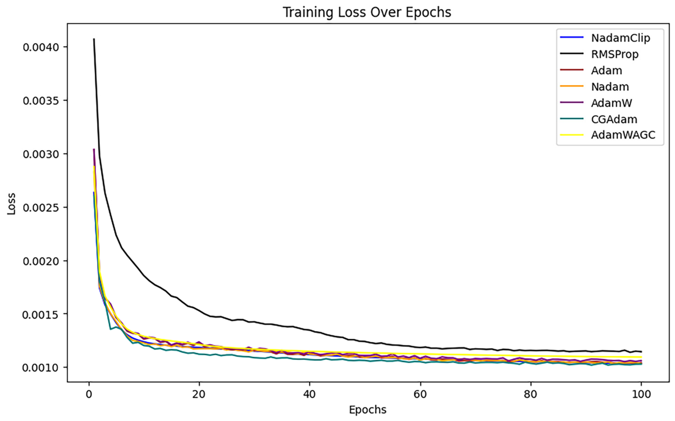
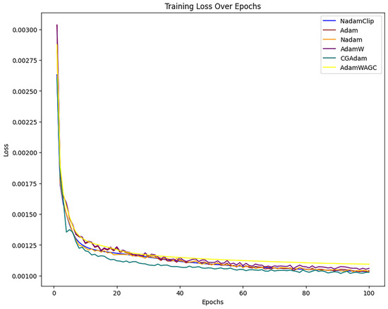
Figure A2.
Comparison of training losses for NadamClip, Adam, Nadam, AdamW, CGAdam, and AdamW_AGC.
Figure A2.
Comparison of training losses for NadamClip, Adam, Nadam, AdamW, CGAdam, and AdamW_AGC.

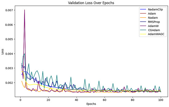
Figure A3.
Comparison of validation Losses for NadamClip, RMSProp, Adam, Nadam, AdamW, CGAdam, and AdamW_AGC.
Figure A3.
Comparison of validation Losses for NadamClip, RMSProp, Adam, Nadam, AdamW, CGAdam, and AdamW_AGC.
References
- Prakash, A.; Khanam, S. Nitrogen Pollution Threat to Mariculture and Other Aquatic Ecosystems: An Overview. J. Pharm. Pharmacol. 2021, 9, 428–433. [Google Scholar] [CrossRef]
- Kaur, G.; Basak, N.; Kumar, S. State-of-the-Art Techniques to Enhance Biomethane/Biogas Production in Thermophilic Anaerobic Digestion. Process Saf. Environ. Prot. 2024, 186, 104–117. [Google Scholar] [CrossRef]
- Wang, S.; Lin, Y.; Jia, Y.; Sun, J.; Yang, Z. Unveiling the Multi-Dimensional Spatio-Temporal Fusion Transformer (MDSTFT): A Revolutionary Deep Learning Framework for Enhanced Multi-Variate Time Series Forecasting. IEEE Access 2024, 12, 115895–115904. [Google Scholar] [CrossRef]
- He, Y.; Huang, P.; Hong, W.; Luo, Q.; Li, L.; Tsui, K.-L. In-Depth Insights into the Application of Recurrent Neural Networks (RNNs) in Traffic Prediction: A Comprehensive Review. Algorithms 2024, 17, 398. [Google Scholar] [CrossRef]
- Rosindell, J.; Wong, Y. Biodiversity, the Tree of Life, and Science Communication. In Phylogenetic Diversity: Applications and Challenges in Biodiversity Science; Springer: Cham, Switzerland, 2018; pp. 41–71. [Google Scholar] [CrossRef]
- Marshall, N.; Xiao, K.L.; Agarwala, A.; Paquette, E. To Clip or Not to Clip: The Dynamics of SGD with Gradient Clipping in High-Dimensions. arXiv 2024, arXiv:2406.11733. [Google Scholar] [CrossRef]
- Mai, V.V.; Johansson, M. Stability and Convergence of Stochastic Gradient Clipping: Beyond Lipschitz Continuity and Smoothness. In Proceedings of the 38th International Conference on Machine Learning, Virtual, 18–24 July 2021; Volume 139, pp. 7325–7335. [Google Scholar]
- Zhang, J.; Karimireddy, S.P.; Veit, A.; Kim, S.; Reddi, S.; Kumar, S.; Sra, S. Why Are Adaptive Methods Good for Attention Models? Adv. Neural Inf. Process. Syst. 2020, 33, 15383–15393. [Google Scholar]
- Seetharaman, P.; Wichern, G.; Pardo, B.; Roux, J. Le Autoclip: Adaptive Gradient Clipping for Source Separation Networks. In Proceedings of the 2020 IEEE 30th International Workshop on Machine Learning for Signal Processing (MLSP), Espoo, Finland, 21–24 September 2020; pp. 1–6. [Google Scholar] [CrossRef]
- Liu, M.; Zhuang, Z.; Lei, Y.; Liao, C. A Communication-Efficient Distributed Gradient Clipping Algorithm for Training Deep Neural Networks. Adv. Neural Inf. Process. Syst. 2022, 35, 26204–26217. [Google Scholar]
- Tang, X.; Panda, A.; Sehwag, V.; Mittal, P. Differentially Private Image Classification by Learning Priors from Random Processes. Adv. Neural Inf. Process. Syst. 2023, 36, 35855–35877. [Google Scholar] [CrossRef]
- Qian, J.; Wu, Y.; Zhuang, B.; Wang, S.; Xiao, J. Understanding Gradient Clipping In Incremental Gradient Methods. Proc. Mach. Learn. Res. 2021, 130, 1504–1512. [Google Scholar]
- Ramaswamy, A. Gradient Clipping in Deep Learning: A Dynamical Systems Perspective. Int. Conf. Pattern Recognit. Appl. Methods 2023, 1, 107–114. [Google Scholar] [CrossRef]
- Dozat, T. Incorporating Nesterov Momentum into Adam. ICLR Work. 2016, 2013–2016. Available online: https://openreview.net/forum?id=OM0jvwB8jIp57ZJjtNEZ (accessed on 1 January 2025).
- Haji, S.H.; Abdulazeez, A.M. Comparison of Optimization Techniques Based on Gradient Descent Algorithm: A Review. PalArch’s J. Archaeol. Egypt/Egyptol. 2021, 18, 2715–2743. [Google Scholar]
- Praharsha, C.H.; Poulose, A.; Badgujar, C. Comprehensive Investigation of Machine Learning and Deep Learning Networks for Identifying Multispecies Tomato Insect Images. Sensors 2024, 24, 7858. [Google Scholar] [CrossRef] [PubMed]
- Kuppusamy, P.; Raga Siri, P.; Harshitha, P.; Dhanyasri, M.; Iwendi, C. Customized CNN with Adam and Nadam Optimizers for Emotion Recognition using Facial Expressions. In Proceedings of the 2023 International Conference on Wireless Communications Signal Processing and Networking (WiSPNET), Chennai, India, 29–31 March 2023. [Google Scholar]
- Pang, B.; Nijkamp, E.; Wu, Y.N. Deep Learning With TensorFlow: A Review. J. Educ. Behav. Stat. 2020, 45, 227–248. [Google Scholar] [CrossRef]
- Kanai, S.; Fujiwara, Y.; Iwamura, S. Preventing Gradient Explosions in Gated Recurrent Units. Adv. Neural Inf. Process. Syst. 2017, 30, 436–445. [Google Scholar]
- Botchkarev, A. Performance Metrics (Error Measures) in Machine Learning Regression, Forecasting and Prognostics: Properties and Typology. arXiv 2022, arXiv:1809.03006. [Google Scholar] [CrossRef]
- Jongjaraunsuk, R.; Taparhudee, W.; Suwannasing, P. Comparison of Water Quality Prediction for Red Tilapia Aquaculture in an Outdoor Recirculation System Using Deep Learning and a Hybrid Model. Water 2024, 16, 907. [Google Scholar] [CrossRef]
- Elesedy, B.; Hutter, M. U-Clip: On-Average Unbiased Stochastic Gradient Clipping. arXiv 2023, arXiv:2302.02971. [Google Scholar] [CrossRef]
- Hodson, T.O. Root-Mean-Square Error (RMSE) or Mean Absolute Error (MAE): When to Use Them or Not. Geosci. Model Dev. 2022, 15, 5481–5487. [Google Scholar] [CrossRef]
- Piepho, H.P. An Adjusted Coefficient of Determination (R2) for Generalized Linear Mixed Models in One Go. Biom. J. 2023, 65, 2200290. [Google Scholar] [CrossRef]
- Duchi, J.; Hazan, E.; Singer, Y. Adaptive Subgradient Methods for Online Learning and Stochastic Optimization. J. Mach. Learn. Res. 2011, 12, 2121–2159. [Google Scholar]
- Zeiler, M.D. ADADELTA: An Adaptive Learning Rate Method. arXiv 2012, arXiv:1212.5701. [Google Scholar] [CrossRef]
- Kingma, D.P.; Ba, J.L. Adam: A Method for Stochastic Optimization. arXiv 2015, arXiv:1412.6980. [Google Scholar] [CrossRef]
- Loshchilov, I.; Hutter, F. Decoupled Weight Decay Regularization. arXiv 2017, arXiv:1711.05101. [Google Scholar]
- Nguyen, T.N.; Nguyen, P.H.; Nguyen, L.M.; Van Dijk, M. Batch Clipping and Adaptive Layerwise Clipping for Differential Private Stochastic Gradient Descent. arXiv 2023, arXiv:2307.11939. [Google Scholar] [CrossRef]
- Chezhegov, S.; Klyukin, Y.; Semenov, A.; Beznosikov, A.; Gasnikov, A.; Horváth, S.; Takáč, M.; Gorbunov, E. Gradient Clipping Improves AdaGrad When the Noise Is Heavy-Tailed. arXiv 2024, arXiv:2406.04443. [Google Scholar] [CrossRef]
- Sun, H.; Cui, J.; Shao, Y.; Yang, J.; Xing, L.; Zhao, Q.; Zhang, L. A Gastrointestinal Image Classification Method Based on Improved Adam Algorithm. Mathematics 2024, 12, 2452. [Google Scholar] [CrossRef]
- Sun, H.; Yu, H.; Shao, Y.; Wang, J.; Xing, L.; Zhang, L.; Zhao, Q. An Improved Adam’s Algorithm for Stomach Image Classification. Algorithms 2024, 17, 272. [Google Scholar] [CrossRef]


Disclaimer/Publisher’s Note: The statements, opinions and data contained in all publications are solely those of the individual author(s) and contributor(s) and not of MDPI and/or the editor(s). MDPI and/or the editor(s) disclaim responsibility for any injury to people or property resulting from any ideas, methods, instructions or products referred to in the content. |
© 2025 by the authors. Licensee MDPI, Basel, Switzerland. This article is an open access article distributed under the terms and conditions of the Creative Commons Attribution (CC BY) license (https://creativecommons.org/licenses/by/4.0/).