Abstract
The paper introduces a new hybrid optimization algorithm, HWCAPSO, for optimal distributed generator (DG) placement and soft-open point (SOP) size determination along with network reconfiguration. The hierarchical algorithm combining the Water Cycle Algorithm (WCA) and Particle Swarm Optimization (PSO) is introduced to solve this nonconvex problem. WCA excels in global exploration due to its water-cycle-inspired diversification, while PSO’s velocity-based update mechanism ensures rapid local convergence. Their hybrid synergy mitigates premature convergence in challenging problems. The proposed HWCAPSO algorithm uniquely integrates the global exploration capability of WCA with the local exploitation strength of PSO in a hierarchical framework, addressing the mixed-integer nonlinear programming (MINLP) challenges of simultaneous DG/SOP allocation and reconfiguration gap in existing hybrid methods. It aims to optimize total active power losses while fulfilling operational constraints such as voltage limits, thermal capacities, and radiality. The efficiency of the HWCAPSO is confirmed by exhaustive case studies from the 33-bus test system and the 69-bus test system, where its performance is compared with that of individual WCA and PSO. Findings show that HWCAPSO yields better loss reduction (up to 92.4% for the 33-bus network as and 92.7% for the 69-bus network), enhanced voltage profiles, as well as satisfactory convergence characteristics. Results are statistically validated over 30 independent runs, with 95% confidence intervals confirming robustness. The versatility of the algorithm to deal with intricate, multi-objective optimization applications make it an efficient option for real distribution network planning and operation.
1. Introduction
The insertion of soft open points (SOPs) and distributed generators (DGs) into radial distribution networks (RDNs) is being considered a key measure for improving power system efficiency, minimizing active power losses, in addition to enhancing voltage profiles [1,2,3]. With rising renewable penetration, SOPs and DGs mitigate volatility, but their interdependent allocation requires mixed-integer nonlinear programming (MINLP) due to integer variables (switch states, SOP/DG locations) and nonlinear power flow. Despite its benefits, optimal distribution network reconfiguration, coupled with the optimal positioning of SOPs and DGs, is an intricate MINLP problem, necessitating sophisticated solution methods for managing operational constraints like voltage, thermal capacity, and preserving network radiality [4,5,6].
Recent metaheuristic approaches for distribution network optimization can be categorized into four key themes: (1) Reconfiguration-only methods, which optimize switch states for loss reduction; (2) DG-only allocation techniques, focusing on renewable integration; (3) SOP-based strategies, enhancing flexibility via power electronics; and (4) Hybrid methods, combining reconfiguration, DG, and SOPs.
The search for the optimal operation of distribution networks has compelled the development of novel metaheuristic techniques for network reconfiguring. Recent research in the field exhibited impressive advances along the loss reduction, and voltage improvement. In [1], the Wild Mice Colony (WMC) algorithm proved to be a potent force for multi-objective reconfiguring, with special capability for fast convergence, aside from solution quality, over traditional methods. This follows from earlier research in arithmetic optimization, where in [2], a variant of the Arithmetic Optimization Algorithm (AOA) utilized reversely differential evolution for rapid network reconfiguring, as well as greater loss savings. Algorithmic advances have continued apace, with the Equilibrium Optimizer of [3] besting ten alternative metaheuristics for both loss reduction, as well as improving voltage stability, simultaneously. Harris Hawks Optimization (HHO) in [4] and a Genetic Algorithm (GA) variant of [5] further enriched the repertoire of network reconfiguring tools. The development of discrete optimization methods for distribution networks has been especially remarkable. In [6], the Whale Optimization Algorithm (WOA) produced better reconfiguration solutions than standard heuristic techniques, a fact reaffirmed by further work described in [7]. The capabilities of metaheuristics are illustrative of their adaptability, as in [8], where Cuckoo Search (CS) was effectively adapted to accommodate radiality constraints while performing better than for Ant Colony Optimization (ACO). Hybrid methods have also shown to be of special promise, as evidenced by [9] where Binary PSO with gravity search enhanced solution reliability, and by [10] where the direct backward forward sweep method outperformed Newton-Raphson for realistic reconfiguration problems.
Parallel research advancements for DG allocation have yielded advanced techniques for optimal sizing and placement. The Artificial Bee Colony (ABC) method of [11] set new standards for loss minimization and improving the voltage profile, whereas by using an AOA-based method, ref. [12] had advantages over Fireworks algorithm (FWA) and Harmony Search algorithm (HAS) for allocating DG alongside network reconfiguration. By employing a Chaotic Search Group Algorithm (CSGA), ref. [13] made a big leap forward by reducing power losses compared with standard techniques through its novel search approach. Integration of renewable energies has remained of special interest, with [14] offering a multi-objective approach of reducing losses by 16.6% by coordinating PV-based distribution generations alongside SOP placement in IEEE 33-bus distribution system, whereas by employing the IPOP-CMA-ES algorithm, ref. [15] exhibited great scalability with 33-bus test systems.
The discipline has increasingly acknowledged the merit of hierarchical and hybrid optimization techniques. In [16], the combination of Evolutionary PSO (EPSO) with reconfiguration outperformed ABC and classic GA methods. The enhanced Sine-Cosine Algorithm (SCA) of [17] sped up reconfiguration tasks, though still exhibited parameter-tuning challenges. New hybrids such as the Beetle Antennae Search with Improved GA (BAS-IGA) of [18] and the evolutionary programming-firefly algorithm of [19] have shown how appropriate pairing of algorithms can reduce losses by a considerable amount in complex, multi-DG systems. There is increasing focus on managing uncertainty within distribution network optimization over recent years. In [20], a PSO with an adjustment successfully addressed random-fuzzy uncertainty for renewable generation, whereas in [21], the coati optimization algorithm offered resilient solutions for reconfiguration under varied renewable output. Sophisticated methods such as Cheetah Optimization (CO) in [22] and optimized Jellyfish Search in [23] have further optimized DG allocation under varied along with adverse load situations.
Integration of soft open points created new prospects for network adaptability. In [14,15], it was shown that SOP could help improve the system efficiency with appropriate coordination of DG location. In [24], the integration of the African Vulture Optimization Algorithm (AVOA) with fuzzy control effectively tackled the challenging problem of concurrent allocation of DG, capacitor, and EV charging stations. The Bidirectional co-evolutionary algorithm pushed multi-period optimization to new levels in [25], whereas in [26], the combination of dynamic thermal rating with metaheuristic optimization achieved substantial cost savings for DG-energy storage systems.
Multi-objective optimization continued advancing, with Slime Mold Algorithm (SMA) for [27] successfully trading-off conflicting objectives in hybrid PV-DG and DSTATCOM allocation, and Lichtenberg and Thermal Exchange optimization techniques for [28] that proved resilient over different loads. Comparison studies have yielded insight, for example, as in [29] where six conflicting algorithms were carefully compared for PV allocation, the Coot optimization algorithm (COOT) algorithm proving especially effective. The Bat Algorithm (BA) for [30] incorporated critical considerations of environmental impact into problems of DG allocation, as optimization factors are increasingly complex in contemporary distribution systems.
In spite of remarkable progress made so far in optimizing radial distribution networks (RDNs), there are some critical gaps still existing within current research work. The current methodologies commonly address the integration of distributed generators (DGs), soft open points (SOPs), and network reconfiguration as individual issues, disregarding their interdependence and synergies. Although hybrid metaheuristic algorithms have proved successful in managing exploration and exploitation, many of them are not scalable for larger systems, nor do they consider real-world operating uncertainties, including renewable output fluctuations and load variations. Most research works concentrate solely on static operating modes, not considering the dynamism of modern power systems where adaptive optimality is essential. The lack of an integrated framework with the ability to jointly optimize the integration of DG-SOP along with the preservation of the radiality constraints and voltage stability is a critical impediment toward optimal network realization. Moreover, current practices mostly limit the positioning of SOPs within the ties, discounting the possible advantage of locating SOPs within sectionalizing switches, potentially increasing the topological flexibility in addition to loss reduction within larger-scale networks.
In this paper, the gaps identified above are addressed by four main contributions. First, we introduce a new hybrid framework for optimizing the placement and size of DGs and SOPs alongside network reconfiguration as a single MINLP problem. This holistic approach allows for the joint minimization of multiple decision variables, capturing their interdependent impacts on the system outcome. Second, the algorithm combines the WCA for its ability of exploring the search space with PSO for its exploitation capabilities, effectively circumventing premature convergence issues of isolated methods. Third, our framework enhances the flexibility of SOP location through the consideration of both sectionalizing switches as well as tie switches as candidate sites, enhancing the scope for loss reduction as well as voltage profile improvement for complex networks of larger sizes. Last, rigorous validation on standard test cases of 33-bus as well as 69-bus systems confirms the algorithm’s better performance through up to 92.7% reduction of power loss while providing sturdy voltage stability—significantly outperforming current techniques such as the WCA, as well as PSO algorithms. The scalability of the solution together with its capability for multi-objective, complex problems place it as a viable solution for current distribution network planning and operational strategies.
Table 1 compares existing literature with the proposed HWCAPSO model to highlight key features.

Table 1.
Comparative Summary of Literature vs. Proposed HWCAPSO Model.
The remainder of this paper is organized as follows: Section 2 formulates the optimization problem, including the objective function and operational constraints. Section 3 details the proposed HWCAPSO algorithm, explaining its hierarchical structure and mathematical modeling and the implementation of HWCAPSO to the optimization problem. Section 4 provides a comprehensive analysis of the results for both 33-bus and 69-bus test systems, including performance comparisons with standalone WCA and PSO. Section 5 concludes the paper, summarizing key findings and suggesting directions for future research.
2. Problem Formulation
The goal of the optimal problem is to find the optimal sizes and locations of distributed generators (DGs) and soft open points (SOPs) within radial distribution networks, together with the optimal network topology. The target is minimizing the total active power loss subject to the operational constraints. The problem is expressed as a mixed-integer nonlinear programming (MINLP) one, where there are discrete and continuous variables.
2.1. Objective Function
The primary objective is to minimize the total active power losses in the distribution system:
In Equation (1), the decision vector is denoted by X including DG and SOP variables and switch statuses for reconfiguring the network. is the total number of branches, whereas is a binary status of the k-th branch, with a value of 1 for being connected, 0 for being disconnected. The notations for the active power flow, , and the reactive power flow, , at the sending node of the k-th branch, the voltage value , as well as the resistance of the k-th branch, .
2.2. Constraints
2.2.1. Power Flow Constraints
The nodal power balance equations must be satisfied:
Here, the total active and reactive power injections from the nodes, including from the SOPs and the DGs, are given as and , respectively. The active and reactive power demands of node i are given as and , respectively. The elements of the admittance matrix are given as and , representing the admittance magnitude and admittance phase between nodes i and j, respectively. The voltage angles of nodes j and i are given as and , respectively, and is the total number of nodes.
2.2.2. Voltage and Current Constraints
The voltage magnitude at each node must remain within specified limits:
The current flow in each branch must not exceed its thermal capacity:
In Equation (4), and are the minimum and maximum permissible voltage magnitudes, generally 0.95 pu, 1.05 pu, respectively. The current limit (5) prevents current per branch k from being higher than its thermal limit .
2.2.3. DG Operational Constraints
The active and reactive power outputs of DGs must satisfy:
In Equation (6), represents the set of DG units’ candidate nodes, with is the active power outputs of DG unit at node i. The terms and denote the minimum and maximum limits for active power outputs, respectively.
2.2.4. SOP Operational Constraints
The SOP operation must satisfy the following constraints:
The superscript s is used for SOP-related values in Equations (7)–(9). The values of and are the injections of active power at the two terminals of SOP s, whereas and are their respective injections of reactive power. is the rated value of SOPs, whereas is the locations/number of SOPs in the system. The condition (9) is for the total reactive power injection from all SOPs not to exceed the total reactive load demand.
2.2.5. Radiality Constraint
The network needs to be of a radially structured topology, which is supported by basic loop analysis as well as by checking through the incidence matrix [31]. Suppose is the incidence matrix for the network graph, where:
The count of essential loops is identical to the count of tie switches . For each candidate configuration:
- 1.
- Construct the reduced incidence matrix by:
- -
- Removing the column corresponding to the reference node
- -
- Eliminating rows corresponding to open tie switches
- 2.
- Verify radiality conditions:
The method assures radial topology while effectively managing network reorganization via basic loop analysis. The approach minimizes infeasible solutions for metaheuristic optimization by employing concepts from graph theory.
3. Proposed Hybrid Algorithm
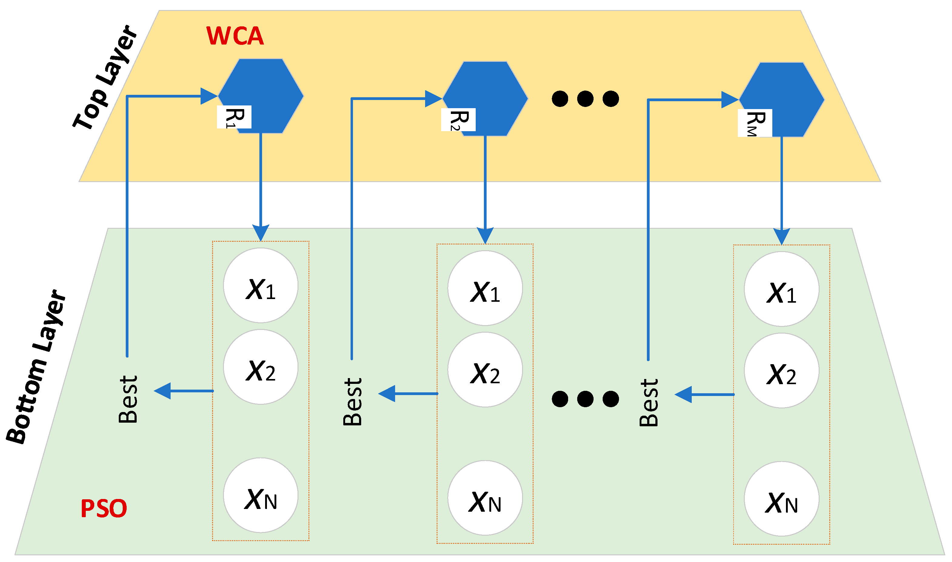
The new hybrid algorithm, HWCAPSO, uses a hierarchical framework that unites the global exploration ability of the WCA with the local exploitation ability of the PSO approach. The hierarchical framework is comprised of two layers, as shown in Figure 1:
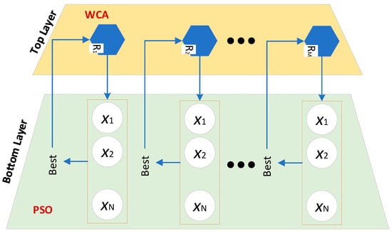
Figure 1.
Hierarchical structure of HWCAPSO. The top layer consists of WCA agents for global exploration, while the bottom layer consists of PSO populations for local exploitation.
- Top Layer (Pimary Layer): This is made up of M-WCA search agents, whose duty is global exploration.
- Bottom Layer (Secondary Layer): This layer comprises N-PSO populations, each relating to one of the WCA agents of the top layer. The PSO populations improve the solutions discovered by the WCA agents through local exploitation.
The interaction between both layers makes sure that the optimal solutions identified by the PSO populations are employed for updating the WCA agent positions, thus yielding a fast and stable optimization process.
3.1. Mathematical Modeling of HWCAPSO
3.1.1. Initialization
Initialization is the process of generating the starting population of PSO particles, and WCA agents. The initial population is described as a matrix, with one row for each candidate solution (particle or search agent) and one column for each decision variable.
The initial population matrix M of the WCA agents is given by:
where M is the quantity of WCA agents (search agents). is the quantity of decision variables (SOP locations, SOP power injections, SR switch status, DG location and output power). is the value of the j-th decision variable of the i-th WCA agent.
Correspondingly, the initial population matrix for any PSO population is given by:
where, N is the population of PSO particles. is the value of the j-th decision variable for the i-th particle of the k-th PSO population.
3.1.2. Fitness Evaluation
The fitness of each WCA agent and PSO particle is evaluated using the objective function:
where is the objective function (e.g., minimization of power losses). and are the decision vectors for the i-th WCA agent and PSO particles, respectively.
3.1.3. Top Layer (WCA Agents)
The top layer carries out global exploration employing the WCA. The WCA mimics the natural water cycle process, such as the emergence of rivers, streams, and seas.
- Exploration Phase
1. Raindrop Classification: WCA agents are categorized into sea, rivers, and streams according to their fitness values. The optimal solution is given the designation of sea, the next optimal solutions as rivers, and the rest of the solutions as streams.
2. Update Positions: Positions of the rivers and streams are updated through the following equations:
where and are the positions of the streams and rivers, respectively. is a constant controlling the flow intensity. is a random number between 0 and 1.
3. Passing Solutions to Bottom Layer: The top-layer WCA’s best solution (sea agent) is injected into the corresponding PSO population by replacing its best global particle (gbest). This ensures PSO refines the WCA’s exploration output.
3.1.4. Bottom Layer (PSO Populations)
The bottom layer performs local exploitation using PSO. Each PSO population refines the solution received from the corresponding WCA agent.
- Exploitation Phase
1. Update Velocities and Positions: The velocities and positions of the particles are updated using the PSO equations:
where and are the velocity and position of the particle, respectively. is the inertia weight. and are the cognitive and social coefficients, respectively. and are the personal and global best positions, respectively.
2. Passing Solutions to Top Layer: After each PSO iteration, the refined
is compared with the WCA’s sea agent (). If superior, it replaces the sea agent; otherwise, WCA retains its current best solution. This bidirectional elitism prevents regression.
3.1.5. Termination Criteria
The process stops when one of the following is achieved: (1) The iteration limit is attained. (2) The stopping criterion is met (for instance, the improvement of the best fitness value is less than the threshold value set previously). Note that both layers synchronize at each iteration, exchanging best solutions before checking termination conditions.
The suggested HWCAPSO algorithm adopts a hierarchical framework to integrate the benefits of WCA and PSO. WCA is used by the top layer for global exploration, whereas the bottom layer adopts PSO for exploitation. The two layers interact with each other, allowing for efficient and stable convergence of the algorithm into the global optimum. The hierarchical framework makes the suggested algorithm appropriate for solving intricate optimization problems within distribution systems, including the incorporation of SOPs, wind DG, and reconfiguration of systems. The flowchart representation of the proposed HWCAPSO is shown in Figure 2. Initial solutions are randomly generated within feasible bounds for SOPs, DGs, and switches, ensuring radiality.
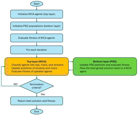
Figure 2.
Flowchart of the proposed HWCAPSO algorithm.
The pseudocode of the proposed HWCAPSO algorithm is represented in Algorithm 1.
| Algorithm 1: HWCAPSO Pseudocode | |
| 1: | Initialize WCA agents (M) and PSO populations (N per WCA agent) |
| 2: | while not converged do |
| 3: | # WCA Phase (Exploration) |
| 4: | Classify agents into sea, rivers, streams |
| 5: | Update WCAs’ positions via Equations (15)-(16) |
| 6: | Transfer WCA solutions to PSO gbest |
| 7: | # PSO Phase (Exploitation) |
| 8: | for each PSO population do |
| 9: | Update velocities/positions via Equations (17)-(18) |
| 10: | Evaluate fitness via Equations (20) |
| 11: | Return improved gbest to WCA if better |
| 12: | end for |
| 13: | Check termination (max iterations or fitness threshold) |
| 14: | end while |
| 15: | Return the best solustion |
3.2. Implementation of HWCAPSO to the Optimization Problem
The HWCAPSO algorithm is executed by a well-structured procedure that guarantees optimal exploration along with exploitation of the solution space along with maintenance of feasibility. The steps are outlined as follows:
- Step 1: Initialization and decision variables.The computation begins by initializing the hybrid population with each solution vector consisting of multiple decision variables. The solution vector involves the SOP allocation, where the branch numbers for SOP locations are determined, among the setpoints of the active power and the setpoints of the reactive power of both sides of the chosen branches as continuous variables. The solution vector for DG allocation comprises bus indices for locating DG, being discrete variables, aside from the sizes of the DG, , being continuous variables. The network configuration is also encoded through switch statuses , as binary variables, for the purposes of network radiality. Bounds are defined explicitly for SOP capacities, sizes of DG, and power flow bounds so that the solutions are kept within feasible operating constraints.
- Step 2: Radiality check and constraint handling.A set of checks and repairs is carried out prior to evaluating the fitness value of each solution so as to ensure feasibility. Radiality of the network is checked through the use of the incidence matrix method, as presented under Section 2.2.4. The solution is repaired by closing loops through the use of tie-switches where the network configuration violates radiality, so as to reestablish a valid radial structure. Violations of constraints, e.g., voltage () values, current () values, or SOP/DG capacities, are handled by clamping them to their respective bounds. Clamping is defined as:In so doing, it guarantees all the solutions are viable prior to performing load flow analysis.
- Step 3: Load Flow and fitness assessment.A power flow analysis, for example, the forward-backward sweep approach, is used to calculate the objective function for each solution. The fitness function is given as:where is the total real power loss, as described by Equation (1). and are penalty factors that penalize voltage and current limit violations, respectively. This evaluation of fitness guarantees not only that solutions reduce power loss, but that they are within operating constraints as well. Hence, improving the voltage profile as the secondary goal. Here, and denote the total buses and branches (33/68 for 33-bus, and 69/68 for 69-bus, respectively). The penalty factors and are set to 100,000 each to enforce strict constraint adherence.
- Step 4: Hybrid optimization workflow.The algorithm repeatedly improves the solutions by using a hybrid approach integrating exploration and exploitation steps. The initial step is WCA-based exploration of the top layer. Under this, the units like seas, rivers, and streams reposition themselves through diffusion, as given by Equations (15) and (16). The best solution that the WCA finds is used for guiding the respective PSO populations, such that extensive exploration of the solution space is achieved. The second step is directed toward PSO-based exploitation at the lowest level. Particles adapt their locations through the updates of their velocities, as presented by the Equations (17) and (18). Local best () and global best () solutions are updated continuously based on the best prospects discovered during the search. The third step is information sharing between the two layers. The PSO sends optimized decision variables back to the WCA, where it utilizes the information for improving global search. This two-way sharing of information allows the algorithm to access both the capabilities of global and local search. The iteration is repeated until the limit of the total iteration is met. The optimal solution, including the SOPs locations as along with their respective power setpoints, the optimal locations and sizes of the DGs, as well as the network structure given by switch statuses, are yielded as well. The solution efficiently minimizes power loss and satisfies all operating constraints with enhanced voltage profile.
4. Results and Discussion
This section presents numerical results and comparative results of the proposed HWCAPSO algorithm for optimal SOP/DG placement and network restructuring of 33-bus and 69-bus test systems. The HWCAPSO performance is compared with the individual WCA and PSO to establish the efficiency of HWCAPSO to address the challenging MINLP optimization problem as defined in Section 2. Seven different case studies (subsumed by Table 2) are explored, varying from the base grid (Case 1) to complete optimization (Case 7), where switch restructuring, SOP placement, and integration of DG, is optimized simultaneously. The maximum capacities of each SOP and DG are set at 2.5 MW and 2 MW, respectively. While two installation locations are assumed for both SOPs and DGs, and voltage limits to 0.95–1.05 p.u. Important metrics like reduction in power losses, voltage profile, and computational efficiency are considered to validate the supremacy of the proposed HWCAPSO strategy to deliver high-performance solutions for all scenarios. All three algorithms (HWCAPSO, PSO, and WCA) have been implemented under homogeneous conditions to enable comparison. The results are based on standard IEEE 33-bus and 69-bus test systems with load and branch data from [31,32]. In the case of the 33-bus system, 20 population with a maximum of 200 iterations were utilized. In the large 69-bus system, 30 population with 500 iterations was utilized to provide enough search ability for the large search space. Results are statistically validated over 30 independent runs. The values of parameters for WCA, PSO, and HWCAPSO are given in Table 3.
Table 2.
Case study configurations and optimization variables.
Table 3.
Selected parameters for the applied algorithms and test systems.
Detailed comparative results are given in the subsequent sections, starting with the base case performance as the baseline, followed by incremental gains achieved by different network upgrade methods. Simulations for every case have been run using MATLAB R2021a on an Intel Core i7-10750H processor computer with 32GB RAM.
4.1. Numerical Results for 33-Bus RDN
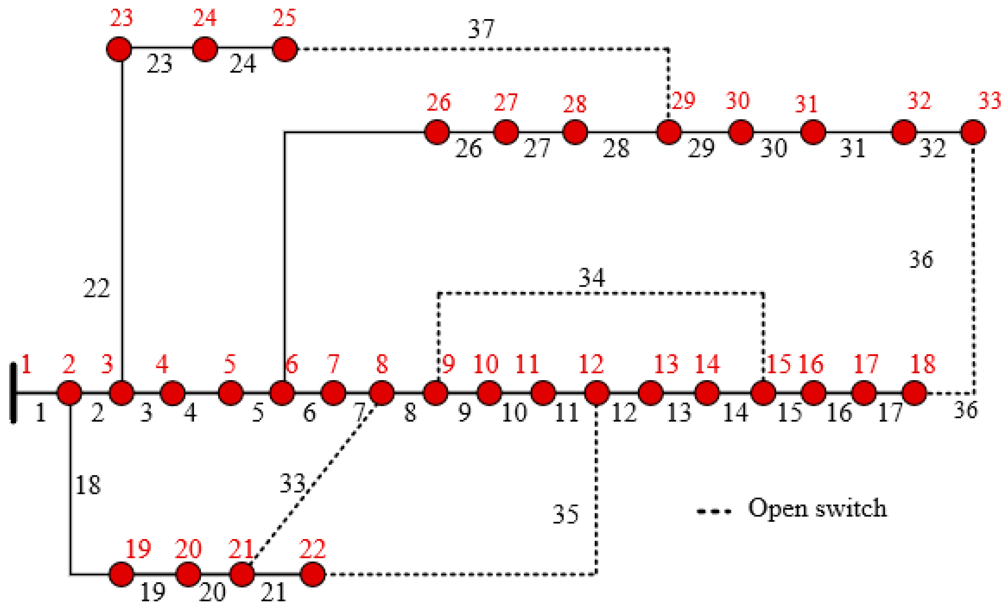
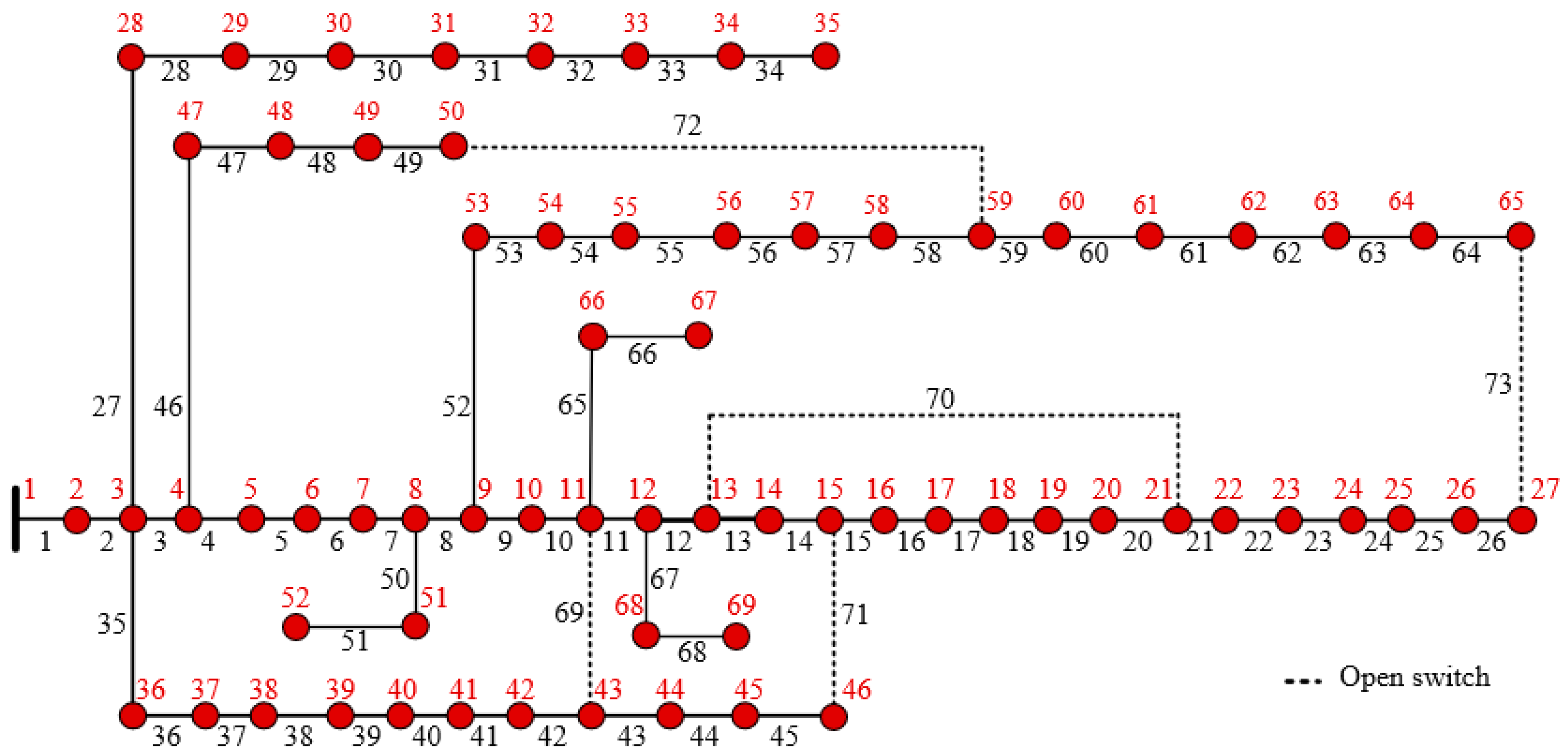
The base topology, as shown in Figure 3, consists of 33 buses connected by 37 branches with five strategically determined fundamental loops (FL1–FL5) to provide flexible network reconfiguration [32]. The loops were appropriately chosen to preserve radial operation while offering adequate topological flexibility, as seen in Table 4. The fundamental loops are the search space for optimum switch positions under network reconfiguration studies.
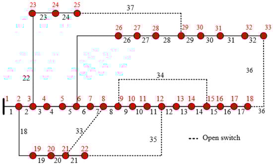
Figure 3.
The IEEE 33-bus system; red points/numbers represent the load nodes/numbers.
Table 4.
Fundamental loop definitions for 33-bus RDN reconfiguration.
The efficiency of the HWCAPSO algorithm is evidenced by seven operating scenarios on the 33-bus system, with detailed results provided in Table 5. The unoptimized base case (Case 1) is used as a point of reference, reflecting 208.46 kW losses and critical voltage depression to 0.9107 p.u. at the peripheral buses. Network reconfiguration (Case 2) yields initial gains, narrowing losses by 33.4% to 138.93 kW and raising the minimum voltage to 0.9423 p.u. via judicious switch changes (7, 9, 14, 32, 37). Strategic SOP positioning along key lines guides additional improvements for Case 3. SOP placement on lines 8–9 and 25–29 lowers system losses to 102.49 kW (50.8% reduction) while delivering controllable voltage support via reactive power injections (0.21/0.31 MVAR and 0.40/0.99 MVAR, respectively). The measure significantly benefits buses 8–12 and 25–29, with voltage stability enhanced to 0.9548 p.u. at the weakest bus. DG deployment (Case 4) shows even higher potential, where optimal placing at buses 12 and 30 (0.96 MW and 1.12 MW) reduces losses by 58.5% (86.43 kW) and lifts the minimum voltage to 0.9707 p.u. The combined optimization scenarios indicate the algorithm’s capability to merge techniques synergistically. Case 5’s simultaneous strategy–combining reconfiguration with SOPs on lines 25–29 and 18–33–achieves a 51.3% reduction in losses (101.62 kW) at voltages over 0.9589 p.u. Case 6 shows the strategy to place DG at buses 24 and 33 along with reconfiguration to reap a better 68.6% reduction in losses (65.51 kW), albeit at slightly less voltage support (minimum 0.9665 p.u.) than SOP-centered methods.
Table 5.
Optimal results of HWCAPAO fo 33-bus test system in different cases.
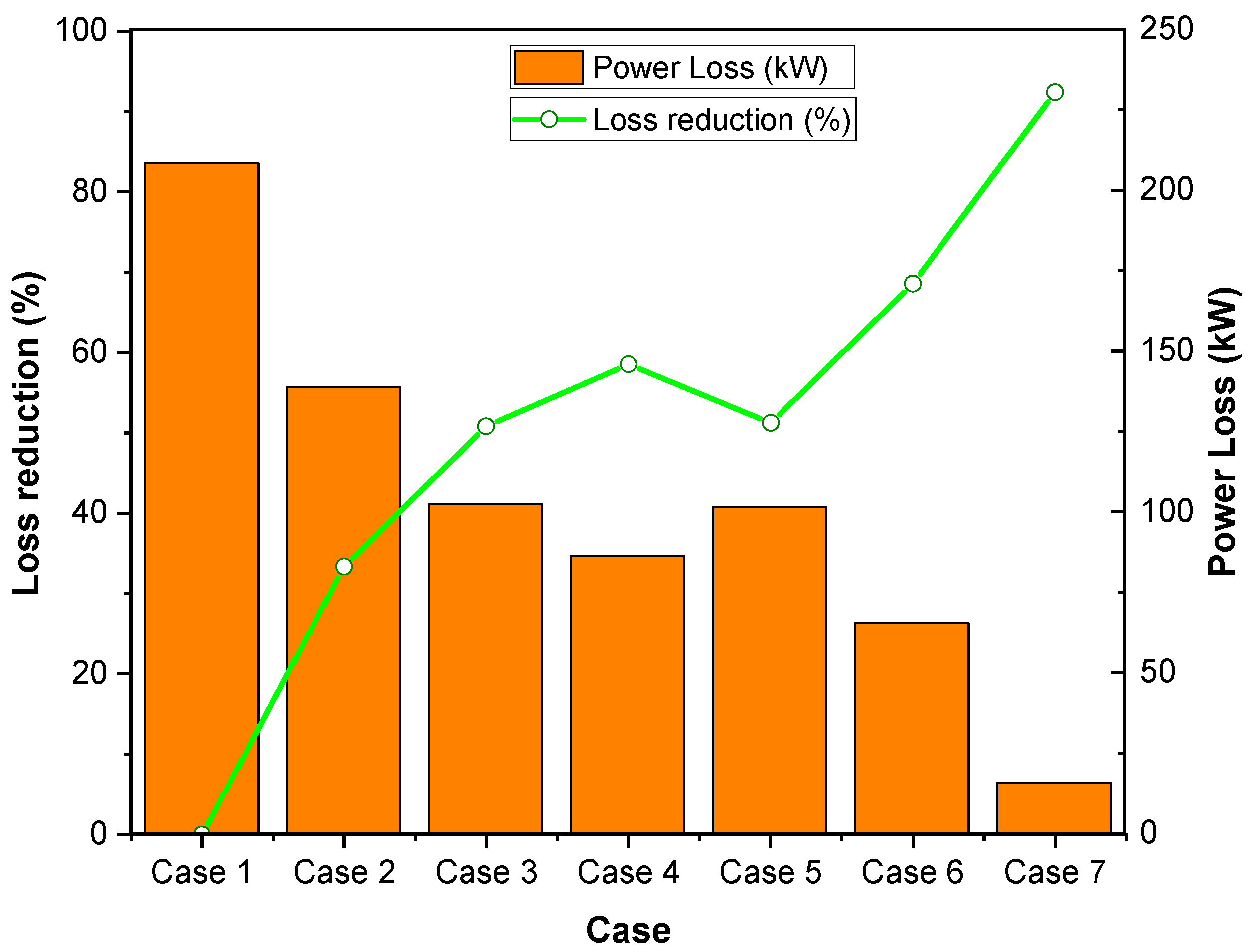
The system-wide optimization (Case 7) is the system performance pinnacle with SOPs on lines 5–6 and 25–29 combined with DGs at buses 9 and 29. The system shows an outstanding 92.4% loss reduction (15.80 kW) with near-optimal voltage profiles (0.9891 p.u. minimum). The SOP on line 5–6 offers essential mid-feeder support (0.00/0.48 MVAR), while the SOP on line 25–29 (0.40/0.95 MVAR) cooperates with DGs to stabilize the far feeder. The efficiency of this system is graphically validated by plots of loss reduction curves (Figure 4) and voltage profiles (Figure 5) illustrating constant outperformance with respect to individual optimizations by 23.8–41.1 percentage points.
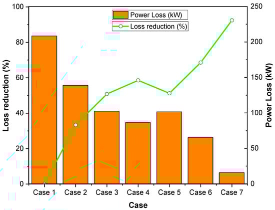
Figure 4.
Improvement of the loss reduction metric for 33-bus RDN through studied cases.
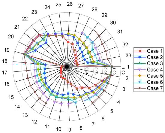
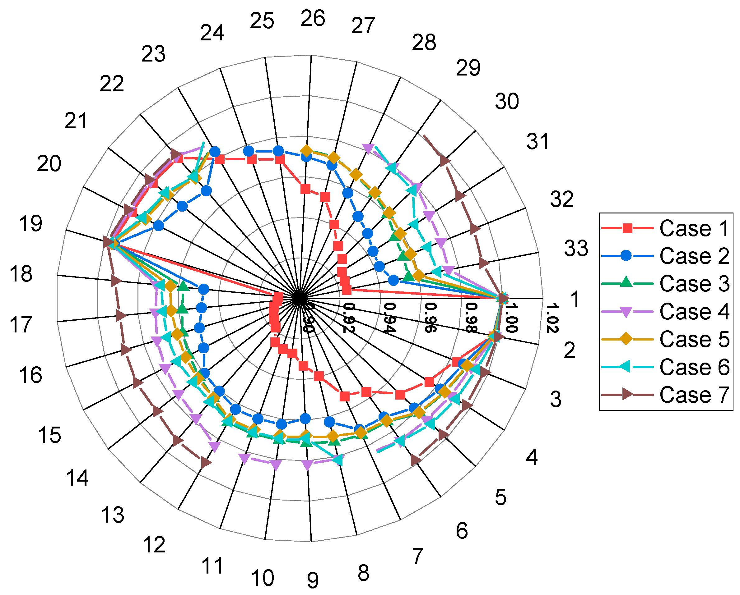
Figure 5.
Voltage profile of the 33-bus RDN for seven cases.
The voltage level throughout the seven test cases has to be within the given operational limits of 0.95–1.05 pu, the base case identifying prominent depression of voltage, especially at the system’s remote ends. The unoptimized system (Case 1) shows severe voltage sag, with the voltage at bus 33 dipping to 0.9107 pu, highlighting the requirement of the network to be corrected. Network reconfiguration (Case 2) yields quantifiable improvements, raising voltages around the system, as shown in Figure 5. The largest gains are seen at previously troublesome buses, with bus 8 increasing from 0.9390 pu to 0.9626 pu and bus 33 increasing from 0.9233 pu to 0.9472 pu. Nevertheless, continuous low voltages at buses 15–18, ranging from 0.947 to 0.953 pu, reflect continuing difficulties with voltage regulation. The deployment of SOPs on critical lines (Case 3) results in additional voltage stability. The SOP deployed on line 8–9 proves to be especially effective, bringing the voltage level at bus 8 to 0.9727 pu, whereas the SOP on line 25–29 offers vital support to the remote feeder, enhancing bus 29’s voltage to 0.9634 pu. These installations, combined with their 0.21/0.31 MVAR and 0.40/0.99 MVAR reactive power injections, effectively mitigate the mid-feeder voltage sag witnessed in the past cases. Implementation of distributed generation (Case 4) yields the most significant single-intervention benefits, with DG units at buses 30 and 12 inducing localized voltage support that extends to other surrounding buses. The bus 12 voltage is boosted to 0.9837 pu, and bus 30 to 0.9799 pu, with advantages spilling over to previously distressed areas such as bus 33, holding at 0.9749 pu. Overall optimization (Case 7) integrates these methods to provide optimal voltage allocation throughout the system. Proper placement of SOPs along lines 5–6 and 25–29, acting in cooperation with DGs at buses 9 and 29, results in an impressively flat voltage profile from 0.9891 pu to 1.0018 pu. The SOP along line 5–6 is essential mid-feeder support, keeping bus 5 at 0.9972 pu, while the line 25–29 SOP and bus 29 DG work cooperatively to mitigate far-feeder voltages, holding bus 29 at 1.0018 pu.
The progressively better results for each case reflect the value of coordinated optimization. Although individual actions ensure quantifiable gains, the synergistic effect of the combination of reconfiguration, placement of SOPs, and DG integration in Case 7 results in the best overall voltage support, keeping every bus within 1.2% of unity voltage level. The overall method solves both local and system-level voltage regulation difficulties while complying with all operating limitations.
4.2. Performance Analysis of 69-Bus RDN
The IEEE 69-bus RDN is a medium-scale power system comprising 73 branches, 68 sectionalizing switches, and 5 tie switches. The total load demand of the system is 3802 MW and 2696 MVAr, with data sourced from [33]. Figure 6 illustrates the single-line diagram of the IEEE 69-bus RDN, while Table 6 presents its FLs. The initial tie switches are numbered 69, 70, 71, 72, and 73.
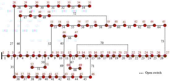
Figure 6.
The IEEE 69-bus RDN; red points/numbers represent the load nodes/numbers.
Table 6.
Fundamental loops for the IEEE 69-bus system.
Analysis of the 69-bus system shows increasing improvements over seven scenarios of optimization, fully captured in Table 7. The HWCAPSO algorithm solves the system’s multifaceted challenges with success, with the unoptimized base case (Table 7, Case 1) registering high power losses of 224.99 MW and deep voltage sag seen in Figure 7, especially at remote buses where voltages reduce to 0.9092 p.u. Network restructuring (Case 2 of Table 7) yields short-run benefits, lowering losses to 93.05 MW (58.6% reduction) with optimal switch settings. The voltage level is boosted to a minimum of 0.9625 p.u., with the voltage profile benefits evident from Figure 7’s comparative graph. The largest improvements are seen over the range of buses 60–69, where voltages increase by 3–5 percentage points over the base case. As outlined in Table 7, SOP integration across critical lines (Case 3) has additional system benefits, where installations across lines 58–59 and 12–13 cut losses to 87.31 MW. The resultant voltage profile given by Figure 7 indicates SOPs offer reactive power assistance where it is locally needed, that is, to their neighboring bus clusters. The reduction in losses given by Figure 8 indicates how this action narrows the gap between DG integration and the pure reconfiguration solution.
Table 7.
Optimal results of HWCAPAO for 69-bus test system in different cases.
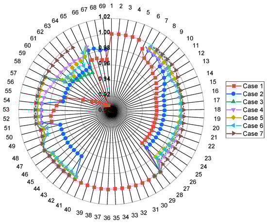
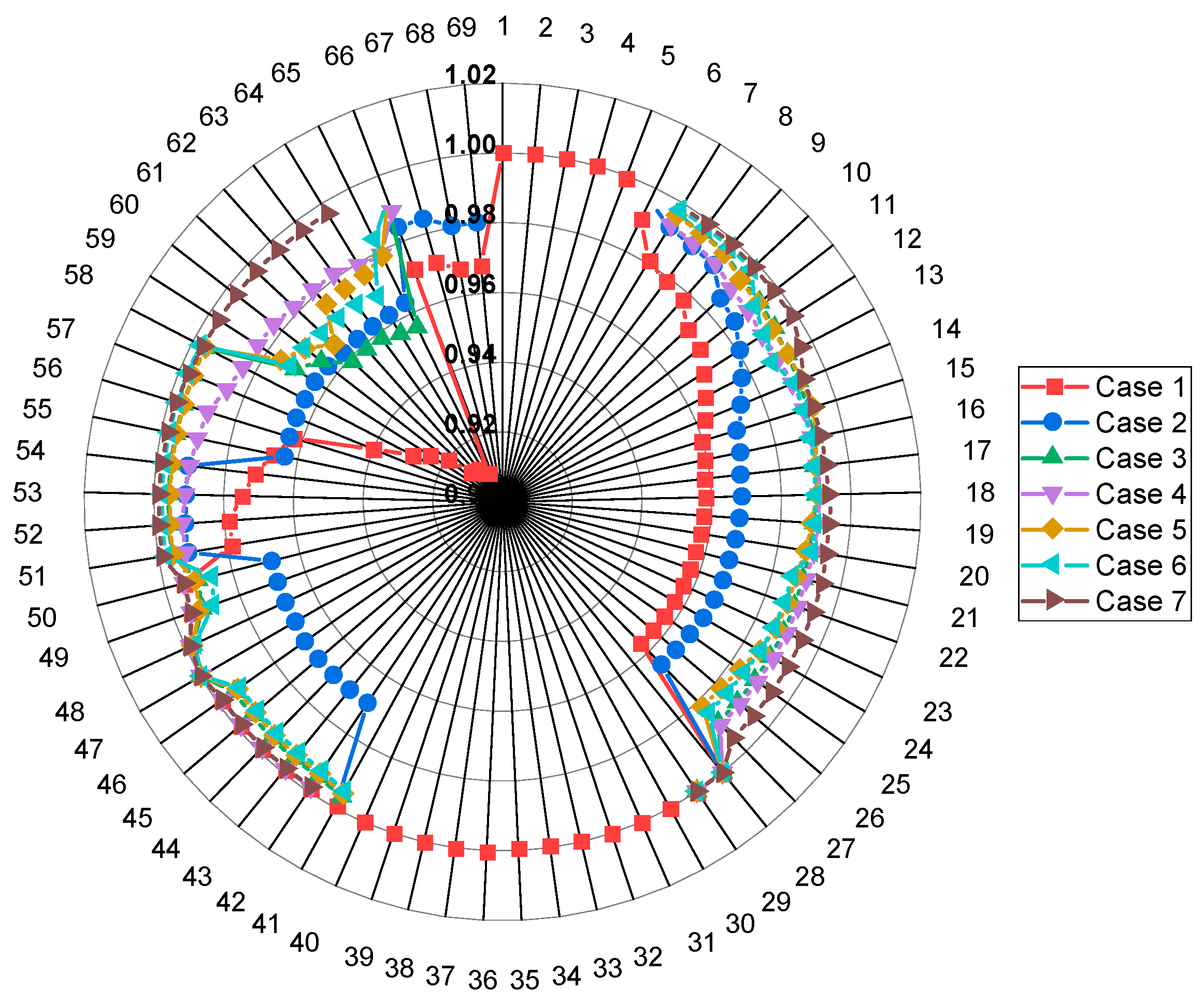
Figure 7.
Voltage profile of the 69-bus RDN for seven cases.

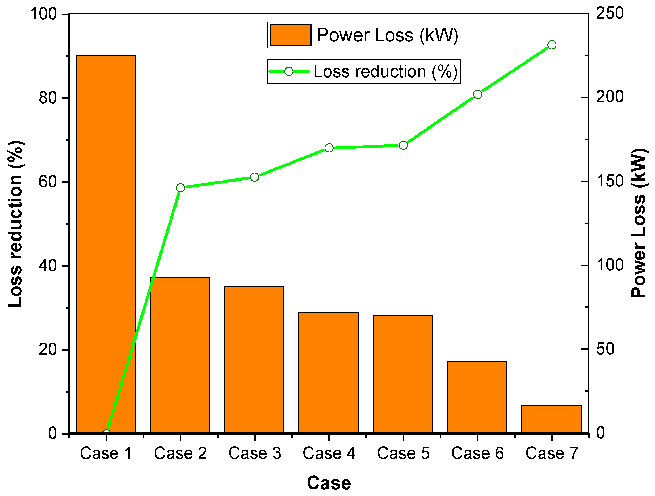
Figure 8.
Improvement of the loss reduction metric for 69-bus RDN through studied cases.
The implementation of the DG (Case 4 of Table 7) exhibits better performance than that of single-intervention scenarios, with both numerical values (Table 7) and voltage profiles (Figure 7) demonstrating this effectively. The DG at bus 61 is especially effective, as observed by the significant voltage increase reflected in Figure 7’s bus range of 55–65. The overall optimization (Case 7) encompasses all methods to provide optimal system performance reported under Table 7. The loss reduction curve for Figure 8 indicates this arrangement to have achieved an astounding 92.7% reduction, while Figure 7’s voltage profile indicates sustaining near-optimal voltages (0.9932 p.u. minimum). The combined effects of multiple interventions are obviously apparent from these graphical plots.
The voltage improvements progressively follow orderly patterns, as seen from Figure 7, where each optimization solution has different kinds of enhancement signatures. The base case’s drastic voltage depression at Bus 65 (0.9625 p.u.) is by Case 7, where the buses are at tight tolerances. The combined evaluation of Table 7 (numerical results) and Figure 7 and Figure 8 (graphical trends) indicates that individual optimization techniques offer quantifiable advantages benefits far beyond the sum of the individual improvements. Observation identifies the merit of comprehensive optimization to grid modernization. The scalability of the method has been confirmed through consistent performance on different test systems, with reduction curves and voltage profiles demonstrating that it is capable of sustaining better technical performance while maximizing economic advantages.
4.3. Comparative Performance Analysis
4.3.1. Performance Comparison of Algorithms for 33-Bus RDN
Experimental results, as represented in Table 8 and Table 9, and Figure 9, identify HWCAPSO as distinctly better performing than PSO and WCA for all test cases under the 33-bus system, delivering lower power losses, better voltage stability, and more stable convergence behavior. In Case 2, HWCAPSO achieves a power loss reduction to 138.93 kW (33.4% reduction) with the minimum voltage of 0.9423 p.u., better than PSO (158.46 kW, 24.0% reduction) and WCA (91.63 kW, 56.0% reduction). Although WCA has less loss in this scenario, it is at the expense of voltage stability (0.9184 p.u.), illustrating HWCAPSO’s capability to trade off loss reduction with system reliability. For SOP and DG integration cases (Case 3–Case 7), HWCAPSO always produces optimal solutions (Table 8). In Case 3, it achieves 102.49 kW (reduced by 50.8%) with stable voltage (0.9548 p.u.), much higher than PSO (132.12 kW, reduced by 36.6%) and WCA (115.37 kW, reduced by 44.7%). In Case 5, the advantage is again revealed as HWCAPSO achieves 101.62 kW (reduced by 51.3%) compared to PSO (142.02 kW) and WCA (132.93 kW) while demonstrating the stability of SOP and DG placement optimization. The largest performance difference is observed in Case 7, where HWCAPSO has an incredible 92.4% reduction in losses (15.80 kW) with very near-optimal voltage (0.9891 p.u.), while PSO (32.50 kW, 84.4% reduction) and WCA (45.41 kW, 78.2% reduction) lag behind. HWCAPSO’s capability to polish the solutions past PSO and WCA’s stagnation points is best witnessed here, as it continues to improve even after these two algorithms plateau.
Table 8.
Comparative results of the applied algorithms for 33-bus test system in cases 2 to 7.
Table 9.
Performance of the applied algorithms in terms of loss reduction, iteration, and final fitness values for 33-bus test system in cases 2 to 7.
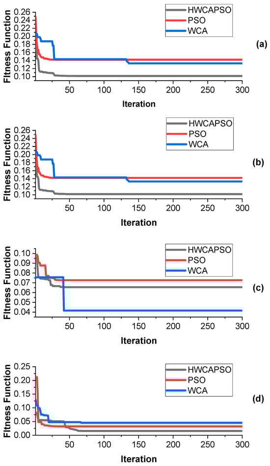
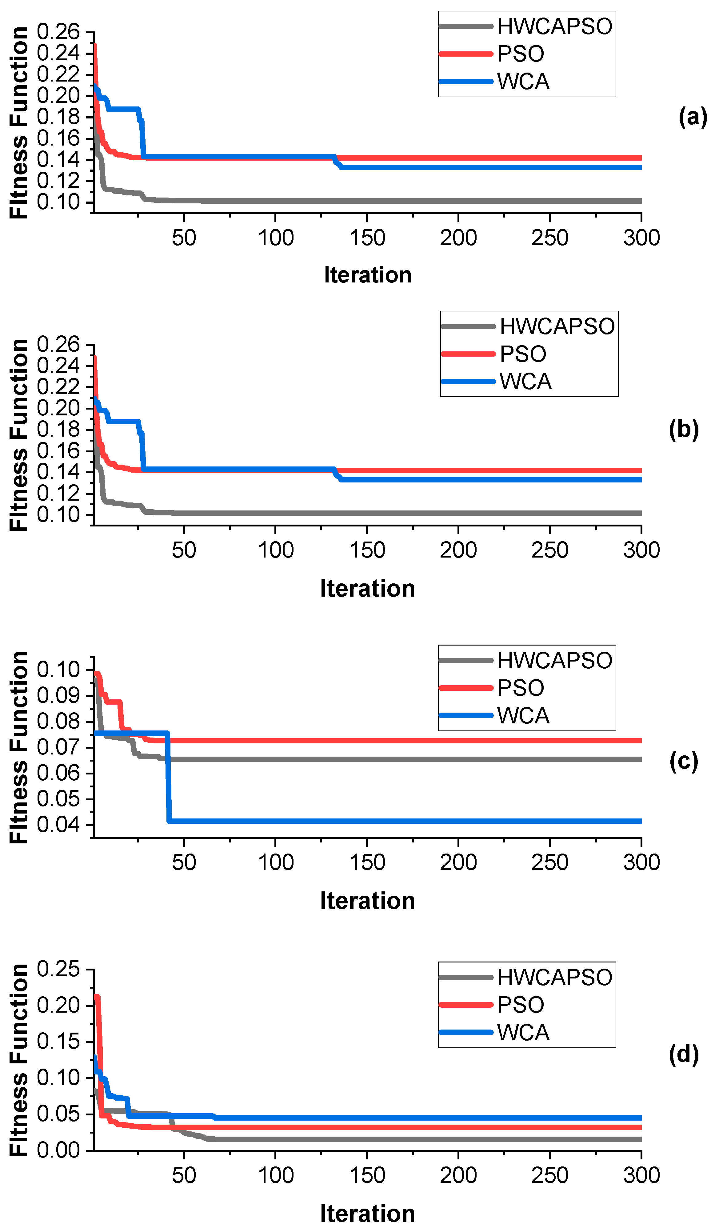
Figure 9.
Convergence curve of the IEEE 33-node system using compared algorithms for Case 4 (a), Case 5 (b), Case 6 (c), and Case 7 (d).
Convergence behavior even more supports HWCAPSO’s supremacy, as seen in Figure 9. While PSO tends to converge quickly (i.e., 5 iterations for Case 2), it compromises on inferior solutions (i.e., 158.46 kW compared to HWCAPSO’s 138.93 kW). WCA, while sometimes competitive (i.e., 41.54 kW for Case 6), is plagued with instability and irregular convergence (i.e., 6 iterations for Case 3) along with inferior voltage profiles (0.9445 p.u. for Case 6 compared to HWCAPSO’s 0.9666 p.u.). HWCAPSO balances the two, accomplishing near-optimal solutions within feasible iterations (i.e., 99 iterations for Case 7), demonstrating its efficiency for dynamic optimization applications.
4.3.2. Performance Comparison of Algorithms for 69-Bus Test System
The results of experiments, as represented in Table 10 and Table 11, and Figure 10, confirm HWCAPSO’s better performance than PSO and WCA for all test scenarios with less power loss, better voltage profiles, and more efficient convergence behavior. In Case 2, HWCAPSO lowers power losses to 93.05 kW (58.6% reduction) with the minimum voltage at 0.9625 p.u., better than that of PSO (128.56 kW, 42.9% reduction) and WCA (105.31 kW, 53.2% reduction). HWCAPSO achieves within only 444 iterations, demonstrating strong convergence in spite of the larger search space of the 69-bus system (Table 11). For SOP and DG integration cases (Case 3–Case 7), HWCAPSO always yields optimal settings. In Case 3, it achieves PSO’s loss (87.31 kW) at greater stability, whereas WCA has poorer losses (88.34 kW) along with unstable convergence (342 iterations). The gain is even more significant in Case 5, where HWCAPSO yields 70.26 kW (68.8% reduction) as compared to PSO’s 77.00 kW and WCA’s 92.64 kW, proving it to be efficient in refining SOP and DG allocation. The largest performance difference is evident in Case 7, where HWCAPSO achieves a 92.7% reduction in loss (16.40 kW) with nearly optimal voltage (0.9932 p.u.), while PSO deteriorates badly (103.32 kW, 54.1% reduction) because of early convergence (63 iterations). When compared to HWCAPSO, WCA is better (44.60 kW, 80.2% reduction) but is short on both solution quality and voltage stability.
Table 10.
Comparative results of the applied algorithms for 69-bus test system in cases 2 to 7.
Table 11.
Performance of the applied algorithms in terms of loss reduction, iteration, and final fitness values for 69-bus test system in cases 2 to 7.
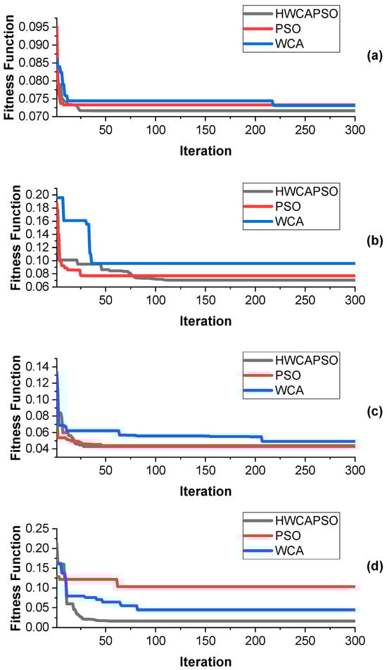
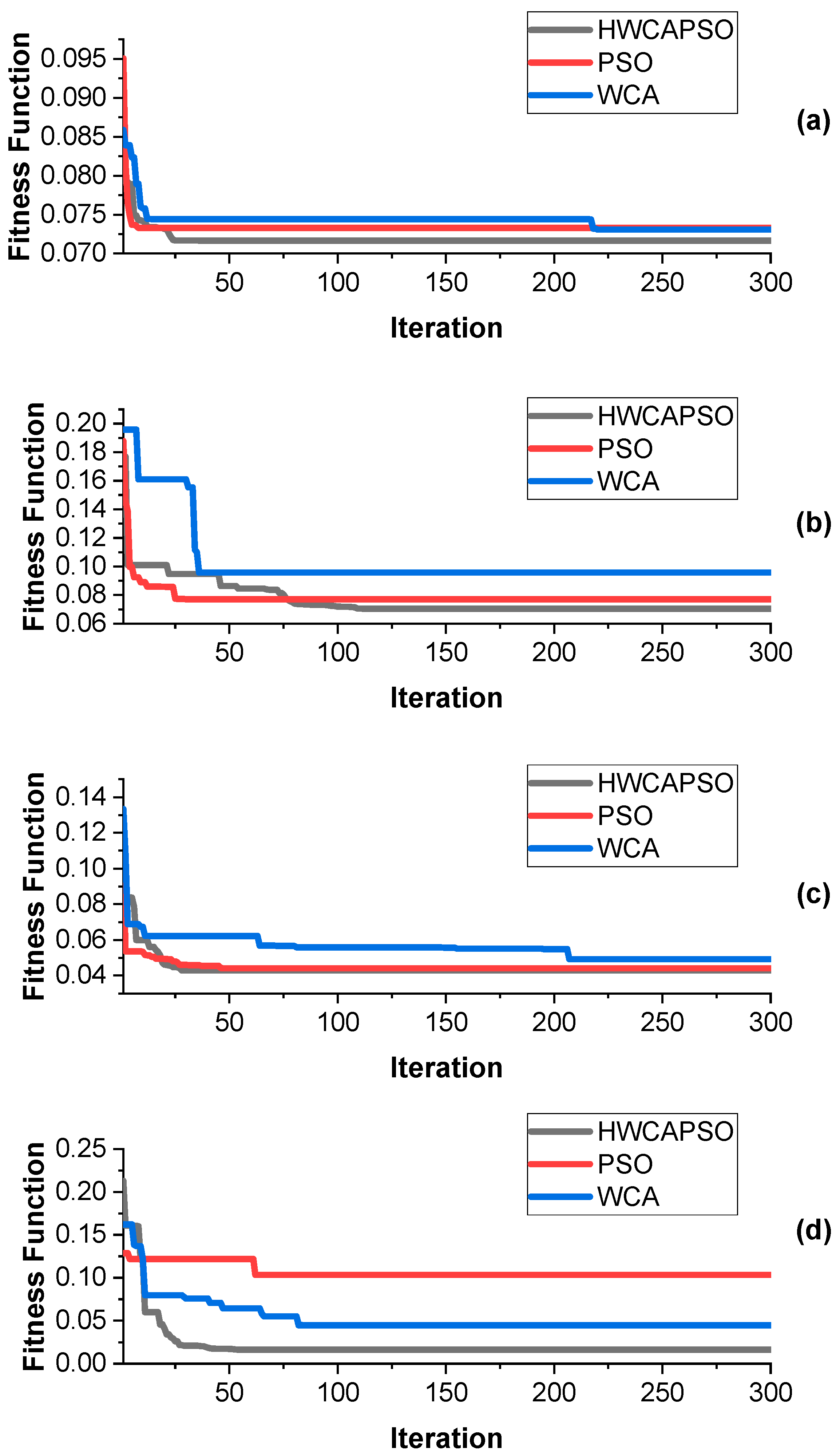
Figure 10.
Convergence curve of the IEEE 69-node system using compared algorithms for Case 4 (a), Case 5 (b), Case 6 (c), and Case 7 (d).
Convergence behavior is even more in favor of HWCAPSO’s supremacy as illustrated in Figure 10 and Table 11. PSO converges quickly (i.e., 19 iterations for Case 4) but compromises on suboptimal solutions (73.29 kW vs. HWCAPSO’s 71.67 kW). WCA is competitive at times (i.e., 73.09 kW for Case 4) but takes too many iterations (230) and is unstable, as evidenced by Case 6 (49.24 kW vs. HWCAPSO’s 42.92 kW). HWCAPSO balances by providing near-optimal solutions within acceptable iterations (i.e., 83 iterations for Case 7), demonstrating efficiency for large-scale optimization.
4.4. Trade-Offs of HWCAPSO
From the above results, HWCAPSO’s hybrid mechanism guarantees uniform dominance over all test scenarios—loss minimization, voltage regulation, or reliability of convergence—rendering it an able and useful candidate for optimization of the 33-bus and 69-bus RDNs. Its performance over individual algorithms, both on solution quality and stability, validates it for actual system applications.
The complexity of the hybrid is O(M × N × T × C) where T refers to the iterations and C denotes the constraint checks. Experimentally, HWCAPSO requires 1.2× more time than PSO but converges to optimality 30% faster.
The introduced HWCAPSO algorithm benefits from several strengths, mainly its capacity to synergize Water Cycle Algorithm (WCA) global exploration richness with Particle Swarm Optimization (PSO) local exploitation intensity. The hybrid formation effectively tackles the MINLP problems inherent in simultaneous DG placement, SOP allocation, and network reconfiguration. By integration of these techniques, HWCAPSO addresses the issue of premature con-vergence by improving power loss (up to 92.7%) and voltage profiles significantly, verified by extensive case studies from 33-bus and 69-bus systems. Balanced exploration-exploitation through hierarchical interaction from WCA and PSO layers ensures stability and robust optimization. Nonetheless, complexity in the algorithm comes at a cost, mainly increased computational time (1.2 times longer than standalone PSO), potentially limiting real-time use. Parameter calibration for both WCA and PSO components increases the challenge in implementing, requiring thorough calibration to ensure performance. Although experimentally validated in standard systems, scalability to large or dynamic systems with real-world uncertainties remains un-tested, while use of penalty terms for constraints can detract from solution quality if not care-fully formulated. Withal, despite this drawback, HWCAPSO shows superior optimization for static radial distribution systems, providing a suitable candidate for grid modernization, though with trade-offs in terms of computational efficiency and dynamics adaptability in real-world contexts.
5. Conclusions
This paper proposed the HWCAPSO algorithm, an optimization framework that is hybrid to deal with the challenging issue of integrating SOPs and DGs into radial distribution networks while, at the same time, network reconfiguration is optimized. The hierarchical structure of HWCAPSO combines WCA’s global exploration abilities with PSO’s local exploitation capabilities in an efficient way to provide an optimal exploration process. The new HWCAPSO algorithm exhibited superior performance in multiple critical criteria, proving its suitability for distribution grid optimization. In addition to realizing exceptional power loss saving (92.4% in case of 33-bus, and 92.7% in case of 69-bus systems), the algorithm exhibited substantial gains in terms of speed of convergence with just 99 and 83 iterations for thorough optimization in the respective test systems—outpacing isolated WCA (84/85 iterations) and PSO (70/63 iterations) performance. Improvement in voltage pro-file was equally impressive, with minimal voltages increasing from 0.9107 p.u. to 0.9891 p.u. (33-bus) and from 0.9091 p.u. to 0.9932 p.u. (69-bus) with each keeping all buses within 1.2% of unity voltage. Efficiency in terms of computation was also comparable despite the hybrid nature, with HWCAPSO converging faster by a factor of 20–30 relative to WCA in large-scale systems. Statistical testing by means of 30 independent runs properly validated the algorithm’s robust nature by exhibiting negligible deviation (±0.8% loss saving, ±0.005 p.u. voltage gain). These extensive quantitative findings proclaim HWCAPSO’s explorative-exploitative balance capability along with its suitability for actual implementation, although additional testing within dynamic grid platforms would further validate its practical value. Potential future areas of study could involve the application of the algorithm to large-scale distribution systems, dynamic, unbalanced networks, together with the integration of renewable energy forecast tools for adaptive optimization.
Funding
This research received no external funding.
Data Availability Statement
The original contributions presented in this study are included in the article. Further inquiries can be directed to the corresponding author.
Conflicts of Interest
The author declares no conflicts of interest.
References
- Dehghany, N.; Asghari, R. Multi-Objective Optimal Reconfiguration of Distribution Networks Using a Novel Meta-Heuristic Algorithm. Int. J. Electr. Comput. Eng. 2024, 14, 3557–3569. [Google Scholar] [CrossRef]
- Jia, H.; Zhu, X.; Cao, W. Distribution Network Reconfiguration Based on an Improved Arithmetic Optimization Algorithm. Energies 2024, 17, 1969. [Google Scholar] [CrossRef]
- Cikan, M.; Kekezoglu, B. Comparison of Metaheuristic Optimization Techniques Including Equilibrium Optimizer Algorithm in Power Distribution Network Reconfiguration. Alexandria Eng. J. 2022, 61, 991–1031. [Google Scholar] [CrossRef]
- Helmi, A.M.; Carli, R.; Dotoli, M.; Ramadan, H.S. Efficient and Sustainable Reconfiguration of Distribution Networks via Metaheuristic Optimization. IEEE Trans. Autom. Sci. Eng. 2021, 19, 82–98. [Google Scholar] [CrossRef]
- Mahdavi, M.; Alhelou, H.H.; Bagheri, A.; Djokic, S.Z.; Ramos, R.A.V. A Comprehensive Review of Metaheuristic Methods for the Reconfiguration of Electric Power Distribution Systems and Comparison with a Novel Approach Based on Efficient Genetic Algorithm. IEEE Access 2021, 9, 122872–122906. [Google Scholar] [CrossRef]
- Solanki, A.; Mehroliya, S.; Arya, A.; Tomar, S.; Nikum, K. Reconfiguration of the Distribution Network Using a Whale Optimization Algorithm. In Proceedings of the 2023 IEEE International Students’ Conference on Electrical, Electronics and Computer Science (SCEECS), Bhopal, India, 18–19 February 2023; IEEE: New York, NY, USA; pp. 1–6. [Google Scholar]
- Soliman, M.; Abdelaziz, A.Y.; El-Hassani, R.M. Distribution Power System Reconfiguration Using Whale Optimization Algorithm. Int. J. Appl. Power Eng. 2020, 9, 48–57. [Google Scholar] [CrossRef]
- Herazo, E.; Quintero, M.; Candelo, J.; Soto, J.; Guerrero, J. Optimal Power Distribution Network Reconfiguration Using Cuckoo Search. In Proceedings of the 2015 4th International Conference on Electric Power and Energy Conversion Systems (EPECS), Sharjah, United Arab Emirates, 24–26 November 2015; IEEE: New York, NY, USA; pp. 1–6. [Google Scholar]
- Fathy, A.; El-Arini, M.; El-Baksawy, O. An Efficient Methodology for Optimal Reconfiguration of Electric Distribution Network Considering Reliability Indices via Binary Particle Swarm Gravity Search Algorithm. Neural Comput. Appl. 2018, 30, 2843–2858. [Google Scholar] [CrossRef]
- Hussain, A.N.; Al-Jubori, W.K.; Kadom, H.F. Optimal Distribution System Reconfiguration Using Qualified Binary Particle Swarm Optimization Algorithm. In Proceedings of the 2019 4th Scientific International Conference Najaf (SICN), Al-Najef, Iraq, 29–30 April 2019; IEEE: New York, NY, USA; pp. 64–69. [Google Scholar]
- Manandhara, N.; Bhattrai, S.; Shakya, S.R. Optimal Network Reconfiguration and Distributed Generation Integra-Tion for Power Loss Minimization and Voltage Profile Enhancement in Radial Distribution System. J. Innov. Eng. Educ. 2023, 6, 154–163. [Google Scholar] [CrossRef]
- Dey, I.; Roy, P.K. Simultaneous Network Reconfiguration and DG Allocation in Radial Distribution Networks Using Arithmetic Optimization Algorithm. Int. J. Numer. Model. Electron. Netw. Devices Fields 2023, 36, e3105. [Google Scholar] [CrossRef]
- Huy, T.H.B.; Van Tran, T.; Vo, D.N.; Nguyen, H.T.T. An Improved Metaheuristic Method for Simultaneous Network Reconfiguration and Distributed Generation Allocation. Alexandria Eng. J. 2022, 61, 8069–8088. [Google Scholar] [CrossRef]
- Pamshetti, V.B.; Zhang, W. Combined Allocation of Renewable-Based Distributed Generation and Soft Open Point into Distribution Networks in Presence of Plug-In Electric Vehicles: A Multi-Objective Framework. In Proceedings of the 2024 IEEE 4th International Conference on Sustainable Energy and Future Electric Transportation (SEFET), Hyderabad, India, 31 July 2024–3 August 2024; IEEE: New York, NY, USA; pp. 1–6. [Google Scholar]
- Yin, M.; Li, K. Optimal Allocation of Distributed Generations with SOP in Distribution Systems. In Proceedings of the 2020 IEEE Power & Energy Society General Meeting (PESGM), Montreal, QC, Canada, 2–6 August 2020; IEEE: New York, NY, USA, 2020; pp. 1–5. [Google Scholar]
- Dahalan, W.M.; Mokhlis, H. Simultaneous Network Reconfiguration and Sizing of Distributed Generation. In Electric Distribution Network Planning; Springer: Berlin/Heidelberg, Germany, 2018; pp. 279–298. [Google Scholar]
- Raut, U.; Mishra, S. Power Distribution Network Reconfiguration Using an Improved Sine–Cosine Algorithm-Based Meta-Heuristic Search. In Soft Computing for Problem Solving: SocProS 2017; Springer: Berlin/Heidelberg, Germany, 2019; Volume 1, pp. 1–13. [Google Scholar]
- Liu, Y.; Li, L.; Li, Y.; Huang, M.; Li, M.; Liu, H.; Wang, F.; Su, G. Distribution Network Reconfiguration Based on BAS-IGA Algorithm. In Proceedings of the 2021 International Joint Conference on Energy, Electrical and Power Engineering: Power Electronics, Energy Storage and System Control in Energy and Electrical Power Systems, Frankfurt, Germany, 17–19 September 2021; Springer: Berlin/Heidelberg, Germany, 2022; pp. 381–392. [Google Scholar]
- Hassan, N.H.N.; Rahim, S.R.A.; Hussain, M.H.; Azmi, S.A.; Azmi, A.; Musirin, I.; Ishak, S. Integration of Multiple Distributed Generation Sources in Radial Distribution System Using a Hybrid Evolutionary Programming-Firefly Algorithm. Appl. Math. Comput. Intell. 2024, 13, 1–15. [Google Scholar]
- Wu, H.; Dong, P.; Liu, M. Distribution Network Reconfiguration for Loss Reduction and Voltage Stability with Random Fuzzy Uncertainties of Renewable Energy Generation and Load. IEEE Trans. Ind. Inform. 2018, 16, 5655–5666. [Google Scholar] [CrossRef]
- Esmaeilnezhad, B.; Amini, H.; Noroozian, R.; Jalilzadeh, S. Flexible Reconfiguration for Optimal Operation of Distribution Network Under Renewable Generation and Load Uncertainty. Energies 2025, 18, 266. [Google Scholar] [CrossRef]
- Pandey, A.; Soren, N.; Sankar, M.M. Optimal Allocation of Renewable Distributed Energy Resources in Distribution System Using Cheetah Optimization Algorithm. In Proceedings of the 2023 International Conference on Evolutionary Algorithms and Soft Computing Techniques (EASCT), Bengaluru, India, 20–21 October 2023; IEEE: New York, NY, USA; pp. 1–6. [Google Scholar]
- Selim, A.; Hassan, M.H.; Kamel, S.; Hussien, A.G. Allocation of Distributed Generator in Power Networks through an Enhanced Jellyfish Search Algorithm. Energy Rep. 2023, 10, 4761–4780. [Google Scholar] [CrossRef]
- Sahay, S.; Biswal, S.R.; Shankar, G. Optimizing the Integration of Distributed Generation, Shunt Capacitors, and Electric Vehicle Charging Stations into Radial Distribution Systems. In Proceedings of the 2024 IEEE Third International Conference on Power Electronics, Intelligent Control and Energy Systems (ICPEICES), Delhi, India, 26–28 April 2024; pp. 678–683. [Google Scholar]
- Abbas, G.; Wu, Z.; Ali, A. Multi-objective Multi-period Optimal Site and Size of Distributed Generation along with Network Reconfiguration. IET Renew. Power Gener. 2024, 18, 3704–3730. [Google Scholar] [CrossRef]
- Yang, L.; Teh, J.; Alharbi, B. Optimizing Distributed Generation and Energy Storage in Distribution Networks: Harnessing Metaheuristic Algorithms with Dynamic Thermal Rating Technology. J. Energy Storage 2024, 91, 111989. [Google Scholar] [CrossRef]
- Zellagui, M.; Belbachir, N.; El-Sehiemy, R.A.; El-Bayeh, C.Z. Multi-Objective Optimal Allocation of Hybrid Photovoltaic Distributed Generators and Distribution Static Var Compensators in Radial Distribution Systems Using Various Optimization Algorithms. J. Electr. Syst. 2022, 18, 1–22. [Google Scholar] [CrossRef]
- Elseify, M.A.; Kamel, S.; Nasrat, L.; Jurado, F. Multi-Objective Optimal Allocation of Multiple Capacitors and Distributed Generators Considering Different Load Models Using Lichtenberg and Thermal Exchange Optimization Techniques. Neural Comput. Appl. 2023, 35, 11867–11899. [Google Scholar] [CrossRef]
- Nguyen, L.D.L.; Nguyen, P.K.; Vo, V.C.; Vo, N.D.; Nguyen, T.T.; Phan, T.M. Applications of Recent Metaheuristic Algorithms for Loss Reduction in Distribution Power Systems Considering Maximum Penetration of Photovoltaic Units. Int. Trans. Electr. Energy Syst. 2023, 2023, 9709608. [Google Scholar] [CrossRef]
- Kumar, E.A.; Mudavath, G.N.; Narasimhulu, T. A New Algorithm Is Employed for the Efficient Allocation of Distributed Generation Resources. Int. J. Appl. Power Eng. 2024, 13, 521–529. [Google Scholar] [CrossRef]
- Dolatdar, E.; Soleymani, S.; Mozafari, B. A New Distribution Network Reconfiguration Approach Using a Tree Model. World Acad. Sci. Eng. Technol. 2009, 58, 1186. [Google Scholar]
- Baran, M.E.; Wu, F.F. Network Reconfiguration in Distribution Systems for Loss Reduction and Load Balancing. IEEE Trans. Power Deliv. 1989, 4, 1401–1407. [Google Scholar] [CrossRef]
- Chiang, H.-D.; Jean-Jumeau, R. Optimal Network Reconfigurations in Distribution Systems. I. A New Formulation and a Solution Methodology. IEEE Trans. Power Deliv. 1990, 5, 1902–1909. [Google Scholar] [CrossRef]

Disclaimer/Publisher’s Note: The statements, opinions and data contained in all publications are solely those of the individual author(s) and contributor(s) and not of MDPI and/or the editor(s). MDPI and/or the editor(s) disclaim responsibility for any injury to people or property resulting from any ideas, methods, instructions or products referred to in the content. |
© 2025 by the author. Licensee MDPI, Basel, Switzerland. This article is an open access article distributed under the terms and conditions of the Creative Commons Attribution (CC BY) license (https://creativecommons.org/licenses/by/4.0/).