Abstract
Laser-induced breakdown spectroscopy (LIBS) is a rapid, cost-effective technique for elemental analysis that enables real-time measurements with minimal sample preparation. However, LIBS datasets are often high-dimensional and imbalanced, limiting the performance of conventional machine-learning models due to small sample sizes. To address this, we propose a novel data augmentation method that generates synthetic samples using normal distribution sampling. This approach is justified by the central limit theorem, since each spectrum in the dataset used in this study results from averaging over 80 measurements per sample, yielding approximately Gaussian-distributed features. We also apply a dimensionality reduction method based on random forest feature importance, selecting features that account for 95% of cumulative importance. This selection reduces model complexity while preserving performance. Using random forest for both feature selection and modeling, our approach achieves superior accuracy for copper and competitive performance for chromium detection in mulberry leaves. Additionally, the selected wavelengths partially match reference lines reported by NIST, supporting model interpretability. These findings highlight the potential of combining data augmentation and machine learning for more robust and interpretable LIBS-based heavy metal detection.
1. Introduction
Heavy metal pollution in water, air, and soil is a persistent environmental threat, with serious implications for human and ecosystem health. These contaminants can accumulate in plants and animals, eventually entering the food chain and posing risks such as kidney, lung, and reproductive cancers [1,2]. Early detection of heavy metals in agricultural systems is therefore critical for ensuring food safety and minimizing long-term exposure.
Traditional analytical techniques, including atomic absorption spectroscopy (AAS) and inductively coupled plasma mass or atomic emission spectroscopy (ICP-MS/AES), offer high sensitivity and accuracy. However, they are costly, require complex sample preparation, and are unsuitable for rapid or on-site analysis. Laser-induced breakdown spectroscopy (LIBS) has emerged as a promising alternative, offering rapid, low-cost, and multi-elemental detection with minimal sample preparation and the potential for field deployment [1,2,3,4].
LIBS has been successfully applied to detect metals such as chromium (Cr) [1,2,3,5,6], copper (Cu) [3,5,6,7], cadmium (Cd) [1,6,8,9], zinc (Zn) [3,6,9], lead (Pb) [6,7,9,10], and nickel (Ni) [3,7] in a variety of environmental and agricultural matrices. Although less commonly studied, LIBS has also been used to detect mercury (Hg) and arsenic (As) [6]. Applications range from assessing heavy metal contamination in soil to analyzing pollutants in aquaculture products [2,3,7], such as saltwater clams and edible algae [9]. In particular, its use in plant analysis has shown promise for assessing heavy metal accumulation in leaves of species such as cabbage, lettuce, and mulberry [1,5,8]. These applications highlight LIBS’s versatility, but also expose methodological gaps, especially in quantitative modeling under conditions of limited data and complex spectral signals.
Despite its advantages, LIBS also presents limitations that must be acknowledged. Matrix effects can impact plasma behavior and spectral signal consistency. Its sensitivity is generally lower than that of ICP-based techniques, and the resulting spectra are complex and high-dimensional, often containing tens of thousands of features per sample. These challenges complicate quantitative modeling and call for advanced data processing strategies. Most LIBS-based studies focus on quantifying the concentration of specific heavy metals in samples. However, another important approach involves classifying samples based on their heavy metal content, distinguishing between healthy and contaminated plants, or categorizing different contamination levels [9].
Despite its practical benefits, LIBS also presents several challenges that can affect its analytical reliability. These include matrix effects, variations in plasma generation, relatively high limits of detection and quantification, and difficulties in achieving quantitative accuracy without appropriate calibration strategies. Nevertheless, recent comparative studies have demonstrated that LIBS, particularly when combined with data processing and multivariate analysis, can yield results comparable to those obtained from traditional techniques, such as ICP-OES, EDX, and LA-TOF-MS [11,12].
This study aims to strengthen LIBS-based detection methods by integrating data augmentation and machine learning. Our approach addresses key LIBS-specific challenges, including the high spectral dimensionality, which affects interpretability and model performance, and the limited number of labeled samples, which constrains the training of robust predictive models. By generating synthetic samples and applying ensemble learning techniques, we aim to improve prediction accuracy, generalization, and model transparency, making LIBS a more viable tool for real-world environmental and agricultural monitoring.
To address these challenges, this paper proposes a methodology that combines synthetic sample generation via normal distribution sampling with machine learning models, particularly random forest, for both feature selection and prediction. Section 2 presents a review of related work. Section 3 details the LIBS dataset, the data augmentation procedure, and the design of the classification and regression models. Section 4 discusses the evaluation of the proposed method, including comparisons between real and synthetic training data and an analysis of feature relevance. Finally, Section 5 summarizes the main contributions and outlines potential directions for future research.
2. Related Work
LIBS data analysis is typically performed using either regression or classification techniques. While both approaches have shown promise, each presents specific limitations and trade-offs that impact their generalizability, complexity, and interpretability. This section critically reviews relevant work, identifying key methodological trends, challenges, and research gaps.
2.1. Regression Approach
Most regression-based LIBS studies rely on multivariate modeling strategies to predict heavy metal concentrations, with simple linear regression (SLR) generally disregarded due to poor performance. As noted in [13], multivariate linear regression (MLR) tends to yield better results, particularly when combined with robust preprocessing and dimensionality reduction.
A typical regression pipeline involves multiple steps: signal preprocessing, feature selection or reduction, model fitting, and validation. However, these steps are often handled using a wide variety of algorithms, making comparisons between studies difficult and undermining model transparency. For example, while normalized autoscaling [8] and Savitzky–Golay smoothing [1] are commonly used to reduce noise, other works employ more complex chains of transformations. The authors in [7] combined logarithmic transformation, MAD filtering, and discrete wavelet transformation—an approach that may increase noise robustness but also adds processing complexity.
Principal component analysis (PCA) has been widely adopted for both preprocessing and dimensionality reduction [5,8,9]. While PCA is effective for compressing high-dimensional spectral data, it often obscures physical interpretability, which can be critical in environmental and agricultural monitoring. In addition, feature selection techniques such as GA, SPA, SOM, UVE, and VIP [5,6,8,14] have been proposed to reduce overfitting, but they are computationally intensive and require tuning, which limits their scalability.
More efficient alternatives, such as the threshold variable (TV) method [6] or intensity-based filtering [15], aim to retain only the most informative wavelengths based on signal characteristics. However, few studies directly compare these simpler methods with established feature selection techniques, making it unclear whether the trade-off in performance is justified. Recent innovations, such as the CCFCV method [16], attempt to enhance variable relevance by cross-referencing selected features with characteristic wavelengths, although its superiority over simpler methods remains context-dependent.
In terms of modeling algorithms, PLSR remains the standard due to its ability to handle collinear data. However, alternative approaches, including PCR, SVR, LASSO, SVM, and LS-SVM, have shown potential for specific metals and matrices [7,14,16]. Nevertheless, these models are typically tested on small datasets (e.g., <100 samples), and the reliance on random train–test splits raises concerns about performance variability [1,6,7,8,9]. Although methods such as the Kennard–Stone algorithm help reduce bias in dataset partitioning, they are underutilized [8].
Moreover, while statistical metrics such as RMSEC, RMSEP, R2c, R2p, and RPD are standard [17,18,19], few studies report the absolute difference (ABS) between calibration and prediction errors, which could offer a more nuanced understanding of model overfitting [5,6,7]. Table 1 summarizes the best-reported results in LIBS regression for heavy metal detection.

Table 1.
Summary of heavy metal detection results using LIBS and regression analysis.
2.2. Classification Methods
Classification models, although less prevalent than regression models in LIBS-based metal detection, offer significant advantages in scenarios where categorizing samples by contamination level is more actionable than quantifying exact concentrations [20,21]. These methods are particularly relevant in agricultural and regulatory contexts, where decision-making often depends on threshold-based groupings.
Unlike regression, classification tasks typically involve discrete output labels. While this simplifies the output interpretation, it places greater demands on feature separability and class balance. Therefore, most classification approaches rely heavily on feature selection and preprocessing to improve signal clarity and minimize intra-class variance.
- RF offers interpretability through feature importance metrics but may suffer from overfitting if not properly regularized, especially with small datasets [8,22].
- KNN, while simple and effective, is highly sensitive to feature scaling and dimensionality, making its performance unstable without rigorous preprocessing [8,9,14].
- PLS-DA and LRC provide useful linear projections but can struggle with nonlinear relationships and overlapping classes [9,14,23,24].
- SRD introduces rank-based evaluation criteria but is less interpretable and harder to generalize beyond specific use cases [9].
Deep learning models such as deep belief networks (DBN) have recently emerged in LIBS-based classification tasks [23,25,26]. These models can automatically extract complex spectral patterns and have achieved higher accuracy in some studies. However, their applicability is limited by the small sample sizes typical of LIBS datasets. Moreover, DBNs lack transparency and demand significant computational resources, which may not be feasible for most labs or in-field implementations.
Across the reviewed studies, preprocessing strategies vary widely. Techniques such as baseline correction, MSC, SNV, and PCA are frequently used [8,9,14], but their effects are not always critically compared, and standardization is lacking. Furthermore, many studies omit a detailed justification for their preprocessing pipeline, which hinders reproducibility.
Regarding evaluation metrics, accuracy remains the most reported measure, although it provides a limited view in the presence of class imbalance. Very few studies report complementary metrics such as precision, recall, or F1-score, which are crucial when contamination classes are underrepresented [27,28]. This raises concerns about the real-world robustness of these models. Table 2 summarizes key classification studies using LIBS for heavy metal detection, highlighting the wide range of models, preprocessing strategies, and reported results.
Table 2.
Summary of heavy metal detection results using LIBS and classification algorithms.
2.3. Gaps and Research Questions
Despite recent advances, two fundamental issues remain pervasive in LIBS-based machine learning studies: data scarcity and spectral dimensionality. Most LIBS datasets contain a limited number of samples, often generated through artificial contamination protocols such as immersion in metal salt solutions [1,5], resulting in high-dimensional datasets with low sample-to-feature ratios and an increased risk of overfitting.
Although dimensionality reduction techniques are widely used, they are not a substitute for larger, more diverse datasets. This limitation forces researchers to adopt complex modeling pipelines involving multiple algorithms for preprocessing, feature selection, and regression or classification, as seen in [5]. These pipelines may improve performance but often obscure how specific wavelengths influence predictions, reducing the interpretability and transparency of the models.
To our knowledge, no previous studies have implemented data augmentation techniques to expand LIBS datasets in heavy metal detection tasks. This represents a significant research gap. By introducing statistically grounded synthetic data generation (e.g., via normal distribution sampling), it is possible to increase training set diversity, reduce the dependence on aggressive dimensionality reduction, and support the development of simpler, more interpretable models.
Based on these gaps, we pose the following research questions:
- Can data augmentation techniques contribute to the development of simpler and more accurate models for LIBS data?
- Are such models interpretable and robust enough for real-world applications?
3. Materials and Methods
The overall methodology adopted in this study is summarized in Figure 1. It consists of six main stages: (i) dataset acquisition using publicly available LIBS spectra of mulberry leaves, (ii) preprocessing through normalization, (iii) data augmentation using normal distribution sampling, (iv) feature selection based on random forest importance values, (v) model training using three machine learning algorithms (LRC, RF, and SVM), and (vi) performance evaluation through classification and regression metrics.
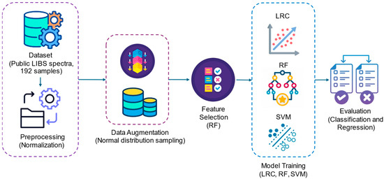
Figure 1.
Overview of the proposed methodology.
3.1. Dataset and Preprocessing
This study aims to leverage data augmentation techniques alongside machine learning algorithms to achieve comparable or superior performance to that reported in [5,16]. The former utilized the same dataset as the present study, while the latter focused on the same heavy metals (Cu and Cr) and sample type (mulberry leaves). Both studies employed regression analysis. Notably, our literature review did not identify any classification studies specifically addressing Cu or Cr detection. This absence may be attributed to the requirement for comparisons with standard spectroscopy schemes, which are costly. Nevertheless, we applied classification algorithms for feature selection and as a benchmark for future research. The performance of regression models was evaluated using R2c, R2p, RMSEC, RMSEP, and ABS, while classification models were assessed based on accuracy.
Two datasets were used, one for chromium and another for copper. Each dataset contains intensity values for five contamination levels, with 20 samples per level, across 22,015 wavelengths. Consequently, each dataset comprises 100 samples and 22,015 features. The dataset is publicly available in [29], where further details on data acquisition can be found.
To provide a clearer overview of the dataset structure and variability, Table 3 presents descriptive statistics of the LIBS dataset used in this study. Each dataset (copper and chromium) consists of 100 samples, each corresponding to a pressed pellet obtained from 0.3 g of mulberry leaf powder. Samples were contaminated with 1 of 5 concentration levels (20 samples per level) and analyzed with LIBS across 22,015 wavelengths. Spectra were averaged from 80 laser-induced measurements per sample. The average intensity and standard deviation across all spectral points were computed to characterize the data distribution.
Table 3.
Summary and descriptive statistics of LIBS dataset for copper and chromium contamination in mulberry leaves.
The spectral data used in this study were originally collected by Yang et al. [5] using a LIBS2000+ system (Ocean Optics, Orlando, FL, USA) coupled with a Q-switched Nd:YAG laser operating at 1064 nm. Fresh mulberry leaves were contaminated by immersion in aqueous CuSO4 and K2CrO4 solutions for 36 h to simulate copper and chromium uptake, respectively. Each sample was pressed into a pellet (10 × 10 × 2 mm, 600 MPa) and analyzed under atmospheric conditions. The laser ablation was performed on 16 positions per sample, with 5 laser shots per position, resulting in 80 individual measurements per sample. The spectra were averaged to reduce variability and improve signal quality, covering a range of 219–877 nm and producing 22,015 data points per sample.
3.2. Data Augmentation Technique
To address data scarcity and improve model robustness, data augmentation was performed using a normal distribution sampling strategy. The method assumes that each spectral feature of the averaged spectra follows an approximately Gaussian distribution, justified by the central limit theorem [30]. This statistical assumption is valid due to the averaging of 80 spectra per sample.
To the best of our knowledge, while data augmentation techniques are common in imaging and text-based machine learning domains, their application to LIBS-based elemental analysis remains scarce. No prior LIBS studies—including [5,6,16]—reported the use of normal-distribution-based sampling to generate synthetic data for model training. Our method addresses this gap by sampling synthetic pseudo-spectra from Gaussian distributions defined by the mean and standard deviation of each feature, grouped by contamination level. This approach preserves spectral variability while maintaining class balance. Figure 2 shows the implemented procedure, which allowed the generation of 500 synthetic samples per metal for model training.
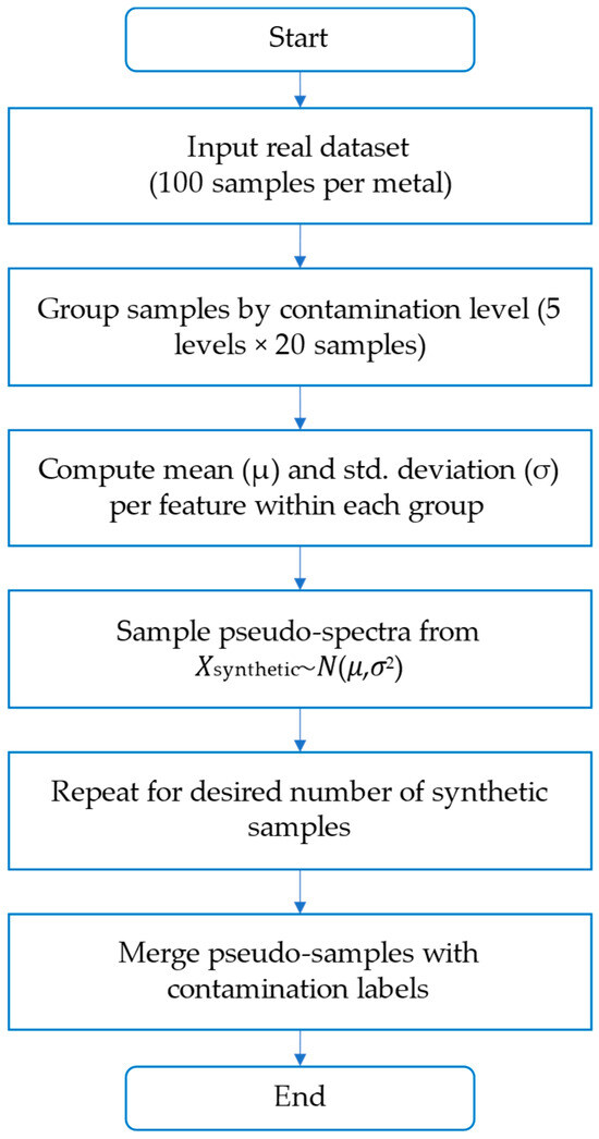
Figure 2.
Flowchart of the data augmentation procedure used in this study.
Pseudo-spectra were generated by sampling from a normal distribution using the mean and standard deviation of each feature within each contamination group. This process enabled the creation of synthetic samples for model training while preserving the structure of the original dataset.
3.3. Machine Learning Models
Most LIBS-based studies rely on regression approaches to predict contamination levels quantitatively [1,5,16]. However, we included classification models for two main reasons:
- To assess the separability of contamination classes using spectral features—an essential step for evaluating whether accurate regression is even feasible.
- To establish a baseline for future classification-oriented LIBS studies, especially since our review revealed no prior classification models targeting Cu or Cr in mulberry leaves.
Moreover, classification helped identify whether the heavy metal levels could be discriminated reliably across contamination categories, supporting feature selection and early screening applications.
We implemented three classification models—random forest (RF), linear regression classifier (LRC), and support vector machine (SVM)—as well as two regression models. Among these, RF was particularly relevant due to its robust ensemble learning capabilities and its ability to evaluate feature importance, which supports both dimensionality reduction and interpretability. More complex models such as gradient boosting regression (GBR), convolutional neural networks (CNNs), and k-nearest neighbors (KNN) were not evaluated in this work primarily to maintain model transparency and due to dataset size constraints. CNNs, for instance, typically require large datasets to avoid overfitting and to fully leverage their feature learning capabilities. Nonetheless, future work could explore the application of these advanced models, particularly in the context of larger, multi-source LIBS datasets, as discussed in the conclusions.
A key novelty of our approach lies in the joint use of data augmentation and RF, applied both as a model and a feature selector. Unlike previous works that rely on multi-stage optimization pipelines, we adopted a single-method strategy for both classification and regression, enabling a more transparent and interpretable modeling process. All the models were trained on the 500 pseudo-samples per metal and tested on the original 100 real samples, using contamination level labels or actual concentrations depending on the task.
For classification tasks, models such as RF, LRC, and SVM were evaluated based on their prediction accuracy, defined as the ratio of correctly classified samples to the total number of samples. In contrast, regression models were assessed using R2c, R2p, RMSEC, RMSEP, ABS, and RPD. This distinction ensures appropriate evaluation of model performance depending on whether the task was classification or regression. In addition to predictive performance and interpretability, computational feasibility was also considered in the model selection process. Given the moderate size of the datasets (n < 1000 samples), all the models (RF, SVM, and LRC) could be trained and tested within reasonable runtimes on standard computing hardware without encountering scalability issues. Therefore, computational cost did not represent a limiting factor in this study.
Among the models evaluated, support vector machine (SVM) offers the advantage of having an explicit mathematical formulation. In classification, SVM seeks the optimal hyperplane that separates the data by maximizing the margin between classes. For a given training set (xi, yi), where xi ∈ ℝn is a feature vector and yi ∈ {−1, +1} is the class label, the linear SVM solves the following optimization problem:
where:
w is the weight vector orthogonal to the separating hyperplane.
b is the bias term (offset).
xi is the i-th input feature vector.
yi is the label of the i-th sample (either +1 or −1).
In our implementation, the scikit-learn SVM classifier was used with default parameters, applying kernel-based decision boundaries when necessary. While our primary focus was model performance, we acknowledge the value of model transparency and reproducibility. Therefore, we consider the use of tools such as WEKA, which can output explicit functional forms for SVM-based regression models, as a valuable addition to future work. Additional implementation details, including the source code for data preprocessing, data augmentation, model training, and evaluation, are provided in the Supplementary Materials (File S1).
4. Results and Discussion
4.1. Evaluation of Data Augmentation Effectiveness
To evaluate the effectiveness of our data augmentation approach, we conducted a series of comparative experiments using the real dataset (without augmentation) and synthetic pseudo-samples generated via normal distribution sampling. These comparisons were designed to assess whether the proposed technique mitigates issues of overfitting or underfitting, and to what extent it improves generalization.
First, an RF classification model was trained using 80% of the dataset (80 randomly selected samples) as the training set, while the remaining 20% was used for testing, establishing a baseline accuracy. Next, the model was trained using an equivalent number of pseudo-samples generated through data augmentation. Finally, the number of pseudo-samples was progressively increased to evaluate its effect on model accuracy.
For the chromium dataset, the baseline accuracy achieved using only real samples was 0.90, with performance remaining stable across different splits. This result indicated a degree of underfitting, likely due to insufficient sample diversity and limited feature variation in the real dataset. Once data augmentation was introduced and at least 215 pseudo-samples were added to the training set, the model’s accuracy improved to 0.95, suggesting that the synthetic data enhanced the classifier’s ability to capture discriminative patterns. It is important to note that the generated pseudo-samples maintained the same distribution across contamination levels. Conversely, for the copper dataset, the baseline accuracy was 1.0, leaving no margin for improvement. When trained with 80 pseudo-samples, the model achieved an accuracy of 0.91, and as the number of pseudo-samples increased to 2100, the accuracy reached 1.0. These results suggest that in this case, training with either real or augmented data yields equivalent performance.
To further validate these findings, k-fold cross-validation (k = 3) was applied to both datasets. When each dataset contained 80 samples, the cross-validation accuracy was 0.8625. However, as the number of pseudo-samples increased, cross-validation accuracy improved accordingly. This highlights a key advantage of this data augmentation approach: the number of pseudo-samples can be freely adjusted to meet experimental needs, whereas real data collection is inherently limited by the feasibility of conducting additional experiments.
In the case of copper, the baseline classification model initially achieved an accuracy of 1.0 on the test set using only real samples. While this result is impressive, it is likely partially attributable to overfitting, given the limited dataset size. The introduction of synthetic pseudo-samples via data augmentation caused a moderate decrease in test accuracy to 0.91, reflecting a more realistic and generalizable performance level. Moreover, three-fold cross-validation experiments showed that the augmented models exhibited more stable accuracy across folds, suggesting that the original perfect accuracy result was sensitive to the limited sampling variability. These findings confirm that data augmentation helps mitigate potential overfitting by enriching the training set diversity.
To further validate that the classification model for copper was not overfitting to noise patterns, we computed a confusion matrix using only real samples for testing and only augmented samples for training. As shown in Figure 3, the random forest model accurately classified most test samples from each contamination level (20 per class), yielding an almost perfect diagonal with only one misclassification. This result supports the claim that the model’s high performance is not due to indiscriminate classification, but rather to its ability to separate spectral patterns across contamination levels. These findings are consistent with the stability observed in cross-validation accuracy reported earlier.
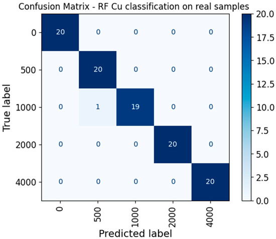
Figure 3.
Confusion matrix for copper classification using a random forest model with an 80/20 train–test split.
A representative LIBS emission spectrum for a copper-contaminated mulberry leaf sample is shown in Figure 4. The most intense emission lines near 324.75 nm and 327.40 nm correspond to characteristic copper transitions. This spectrum was obtained by averaging 80 individual laser-induced measurements, consistent with the dataset used in this study. The illustrated spectral features were considered during model training and feature selection.
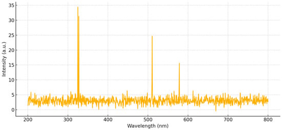
Figure 4.
Representative LIBS emission spectrum for a copper-contaminated mulberry leaf sample.
4.2. Feature Selection and Model Interpretability
Feature selection was performed using the feature_importances attribute of the RF classifier from the scikit-learn package. This method assigns each feature a value between 0 and 1, known as the Gini importance, with the sum of all feature importances equaling 1. To select the most relevant features, we identified the top n features whose cumulative importance reached a predefined threshold of 0.95. Figure 5 and Figure 6 illustrate the cumulative sum of the most significant Gini importance values for the chromium and copper datasets, respectively. The 0.95 threshold was reached with the 500 most important features for chromium and the 300 most important features for copper.
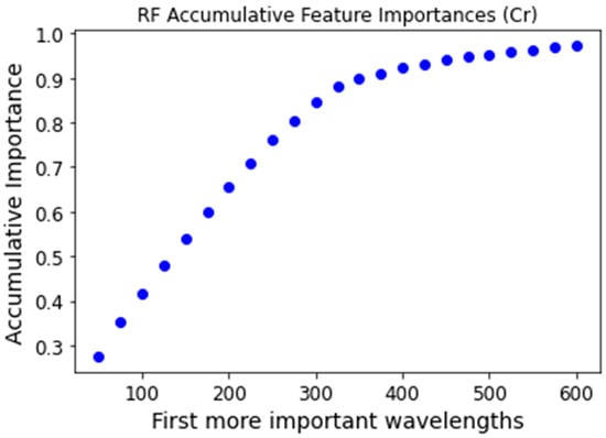
Figure 5.
Chromium accumulative feature importance for the most important features.
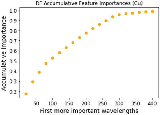
Figure 6.
Copper accumulative feature importance for the most important features.
Beyond feature selection, this approach also enhances model interpretability. Specifically, we investigated whether the selected wavelengths corresponded to those identified by the National Institute of Standards and Technology (NIST). To this end, we examined the overlap between the model-selected wavelengths and NIST-documented wavelengths, applying a ±1% tolerance. NIST reports 91 characteristic wavelengths for copper and 240 for chromium in air [31]. Our models identified 50 and 213 of these wavelengths for copper and chromium, respectively, suggesting that the models exhibit partial interpretability.
The lower matching rate observed for copper (50 out of 91 NIST lines) compared to chromium (213 out of 240 lines) can be attributed to several factors. First, copper spectra in LIBS tend to exhibit lower intrinsic signal-to-noise ratios than chromium under similar acquisition conditions, which can obscure weaker characteristic peaks. Second, overlapping of copper emission lines with background or matrix emissions may reduce the clarity of some features, complicating their identification during feature selection. Lastly, the overall lower variability observed in copper sample intensities may limit the model’s ability to discriminate relevant wavelengths. These aspects highlight the inherent challenges in detecting certain elements and reinforce the need for targeted preprocessing or signal enhancement techniques in future work.
The datasets used for copper and chromium contamination were constructed using standardized contamination levels, spanning five concentration groups for each metal. However, it is important to note that despite the similar design, differences in LIBS spectral characteristics between Cu and Cr were observed. Copper signals exhibited lower average intensities and higher variability in peak strength relative to chromium, potentially due to differences in plasma emission behavior and matrix effects. Moreover, the overlapping of copper emission lines with background noise can obscure weaker peaks and reduce classification or regression performance. These spectral disparities may partly explain the differences in model accuracy observed between the two metals. Figure 7 illustrates the variability of the main LIBS peak intensities for Cu and Cr across the dataset. The variability and lower median intensity observed in copper spectra may contribute to reduced model performance compared to chromium.
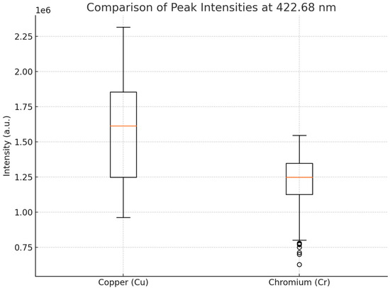
Figure 7.
Boxplot comparison of peak intensities at 422.68 nm for copper (Cu) and chromium (Cr) datasets.
4.3. Model Performance and Comparative Analysis
Three classification models were tested to distinguish between artificial contamination levels: random forest (RF), linear regression classifier (LRC), and support vector machine (SVM). Table 4 summarizes their performance, showing that RF outperformed the other classifiers for both datasets in terms of accuracy. It should be noted that the linear LRC was included in the set of classification models evaluated in this study. However, LRC was not designed for predicting continuous concentration values, and therefore, was not included in the comparison tables for regression models (Table 4 and Table 5). Its performance was evaluated separately within the classification framework.
Table 4.
Classification results.
Table 5.
Chromium regression results.
Additionally, regression analysis was conducted using two approaches: RF and SVM. Table 5 and Table 6 present the regression performance results for the chromium and copper datasets, respectively. As observed, RF achieved the best regression performance in both cases. Notably, SVM yielded a negative coefficient of determination (Table 6), indicating that its regression predictions were unreliable. A negative R2 suggests that the model’s mean squared error (MSE) exceeds the mean total sum of squares (MST), meaning that the regression fit is worse than a trivial baseline represented by a horizontal line at the mean of all training points [32].
Table 6.
Copper regression results.
Table 7 and Table 8 compare the regression models developed in this study with those reported in [5,16]. As shown in Table 7, the copper regression model outperforms all previously proposed models. Notably, our approach employs a single method (random forest) for both feature selection and regression, enhancing model interpretability. Similarly, Table 8 indicates that the chromium regression model achieves performance comparable to that of prior studies. However, our model offers distinct advantages, such as relying on a single algorithm (random forest) and providing greater clarity in its interpretability.
Table 7.
Comparison of copper regression results.
Table 8.
Comparison of chromium regression models.
4.4. Comparison of Real and Augmented Spectra
To assess the realism of the synthetic data generated via normal distribution sampling, we compared representative LIBS spectra from the copper dataset with their corresponding augmented counterparts. Specifically, three real spectra from class 2 were overlaid with three augmented spectra generated from the same class using mean and standard deviation statistics. As shown in Figure 8, the augmented spectra preserve the overall peak structure and intensity profile observed in the real data, while incorporating controlled variability. This result confirms that the data augmentation process respects the physical characteristics of LIBS signals and supports its use as a strategy to enrich small datasets without introducing artifacts.
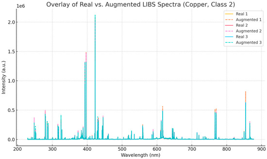
Figure 8.
Overlay of three real and three augmented LIBS spectra from the copper dataset (class 2).
To further support the validity of our data augmentation strategy, we analyzed the intensity histograms for both the real and synthetic samples. Figure 9 (left) presents an example of the distributions for class 3 at a wavelength of 258.51401 nm. The histograms for both the augmented and real data exhibit a shape that resembles the expected bell curve of a normal distribution. Additionally, the Q-Q plots for each distribution are shown in Figure 9 (right). In these plots, the points closely align with a straight line, indicating that both distributions are normal. Furthermore, the intercepts and slopes of the fitted lines are similar, suggesting that the means and standard deviations are also close. This observation reinforces the rationale for using the central limit theorem to justify the application of normal distribution-based sampling for LIBS data augmentation.
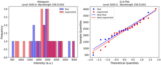
Figure 9.
Real and augmented copper spectra distributions of LIBS intensities (right) and Q-Q plots (left) for class 3 (contamination level: 2000) at wavelength 285.51401 nm.
5. Conclusions
This study evaluated the application of machine learning (ML) models to enhance heavy metal detection through laser-induced breakdown spectroscopy (LIBS), addressing key challenges such as limited sample sizes. Leveraging third-party datasets for copper and chromium detection in plant leaves, a data augmentation strategy based on normal distributions was proposed and validated. The results confirmed that synthetic data generation effectively enriched the training sets, improving model generalization while mitigating potential overfitting. Among the evaluated models, random forest achieved the best performance in both the classification and regression tasks. Feature selection based on Gini importance further enhanced model interpretability, and the agreement of selected wavelengths with National Institute of Standards and Technology (NIST) references validated the physical relevance of the features. Notably, the regression model for copper outperformed previous studies, while the chromium model achieved comparable results with a simpler and more interpretable structure.
Future research could explore alternative dimensionality reduction techniques, such as principal component analysis (PCA), particularly for the chromium dataset, to assess potential performance enhancements. Additionally, applying random forest classification to contamination levels defined by regulatory standards could offer insights into the model’s applicability in real-world scenarios. Further investigation into other data augmentation strategies, such as generative adversarial networks (GANs) and variational autoencoders (VAEs), may provide a comparative assessment of their effectiveness against the normal distribution-based approach.
Another promising direction involves evaluating the generalization capability of the proposed models by testing them on LIBS datasets from diverse sample types, including soil, water, and industrial residues. Incorporating data from independent acquisition campaigns would allow a more robust assessment of model adaptability and minimize potential bias due to limited sampling conditions. Additionally, future studies should analyze the computational scalability of the models when applied to larger LIBS datasets, given the growing availability of high-throughput spectroscopic data. The development and release of open-source code repositories associated with LIBS machine learning pipelines could also enhance reproducibility, foster transparency, and accelerate progress in this field. Finally, integrating hybrid ML models that combine deep learning with traditional approaches could further enhance predictive performance. The implementation of real-time LIBS analysis with embedded ML models represents a significant opportunity to reduce processing time and improve accessibility for environmental monitoring applications.
Supplementary Materials
The following supporting information can be downloaded at: https://www.mdpi.com/article/10.3390/pr13061688/s1. File S1: Source code for data preprocessing, data augmentation, machine learning model training, and evaluation (LIBS_ML_Code_Supplementary.zip).
Author Contributions
Conceptualization, H.C.G.; data curation, C.R.-A. and A.P.; formal analysis, H.C.G. and A.P.; investigation, H.C.G. and C.R.-A.; methodology, H.C.G. and A.P.; validation, H.C.G.; visualization, C.R.-A.; writing—original draft, H.C.G.; writing—review and editing, C.R.-A. and A.P. All authors have read and agreed to the published version of the manuscript.
Funding
This work was supported by Purdue University and Universidad del Magdalena. The APC was funded by Universidad del Magdalena.
Data Availability Statement
The dataset used in this research is available at: Ref. [29], https://doi.org/10.1016/j.dib.2020.106483.
Conflicts of Interest
The authors declare no conflicts of interest.
Abbreviations
The following abbreviations are used in this manuscript:
| AAS | Atomic Absorption Spectroscopy |
| ABS | Absolute Difference Between RMSEC and RMSEP |
| CARS | Competitive Adaptive Reweighted Sampling |
| CV | Cross-Validation |
| CCFCV | Cross Computation Between Full and Characteristic Variables |
| DBN | Deep Belief Networks |
| GANs | Generative Adversarial Networks |
| GA | Genetic Algorithms |
| ICP-MS/AES | Inductively Coupled Plasma Mass/Atomic Emission Spectroscopy |
| KNN | K-Nearest Neighbors |
| KS | Kennard-Stone |
| LIBS | Laser-Induced Breakdown Spectroscopy |
| LASSO | Least Absolute Shrinkage and Selection Operator: |
| LS-SVM | Least Squares Support Vector Machine |
| LDA | Linear Discriminant Analysis |
| LRC | Linear Regression Classifier |
| LVE | Low-Intensity Variable Elimination |
| MAD | Median Absolute Deviation |
| MLR | Multivariate Linear Regression |
| NIST | National Institute of Standards and Technology |
| PLS-DA | Partial Least Squares Discriminant Analysis |
| PLSR | Partial Least Squares Regression |
| PCA | Principal Component Analysis |
| PCR | Principal Component Regression |
| R2c | Coefficient of Determination for Calibration |
| R2p | Coefficient of Determination for Prediction |
| RF | Random Forest |
| RFr | Random Frog |
| RPD | Residual Predictive Deviation |
| RMSE | Root Mean Square Error |
| RMSEC | Root Mean Squared Error for Calibration |
| RMSEP | Root Mean Squared Error for Prediction |
| SOM | Self-Organizing Maps |
| SLR | Simple Linear Regression |
| SPA | Successive Projection Algorithm |
| SRD | Sum of Ranking Differences |
| SVM | Support Vector Machine |
| SVR | Support Vector Regression |
| TM | Threshold Method |
| TV | Threshold Variables |
| UVE | Uninformative Variable Elimination |
| VIP | Variable Importance Projection |
| VAEs | Variational Autoencoders |
References
- Yao, M.; Yang, H.; Huang, L.; Chen, T.; Rao, G.; Liu, M. Detection of Heavy Metal Cd in Polluted Fresh Leafy Vegetables by Laser-Induced Breakdown Spectroscopy. Appl. Opt. 2017, 56, 4070. [Google Scholar] [CrossRef]
- Fu, X.; Ma, S.; Li, G.; Guo, L.; Dong, D. Rapid Detection of Chromium in Different Valence States in Soil Using Resin Selective Enrichment Coupled with Laser-Induced Breakdown Spectroscopy: From Laboratory Test to Portable Instruments. Spectrochim. Acta Part B At. Spectrosc. 2020, 167, 105817. [Google Scholar] [CrossRef]
- Ding, Y.; Xia, G.; Ji, H.; Xiong, X. Accurate Quantitative Determination of Heavy Metals in Oily Soil by Laser Induced Breakdown Spectroscopy (LIBS) Combined with Interval Partial Least Squares (IPLS). Anal. Methods 2019, 11, 3657–3664. [Google Scholar] [CrossRef]
- Ferreira, D.S.; Babos, D.V.; Lima-Filho, M.H.; Castello, H.F.; Olivieri, A.C.; Verbi Pereira, F.M.; Pereira-Filho, E.R. Laser-Induced Breakdown Spectroscopy (LIBS): Calibration Challenges, Combination with Other Techniques, and Spectral Analysis Using Data Science. J. Anal. At. Spectrom. 2024, 39, 2949–2973. [Google Scholar] [CrossRef]
- Yang, L.; Meng, L.; Gao, H.; Wang, J.; Zhao, C.; Guo, M.; He, Y.; Huang, L. Building a Stable and Accurate Model for Heavy Metal Detection in Mulberry Leaves Based on a Proposed Analysis Framework and Laser-Induced Breakdown Spectroscopy. Food Chem. 2021, 338, 127886. [Google Scholar] [CrossRef]
- Su, L.; Shi, W.; Chen, X.; Meng, L.; Yuan, L.; Chen, X.; Huang, G. Simultaneously and Quantitatively Analyze the Heavy Metals in Sargassum fusiforme by Laser-Induced Breakdown Spectroscopy. Food Chem. 2021, 338, 127797. [Google Scholar] [CrossRef]
- Wang, T.; He, M.; Shen, T.; Liu, F.; He, Y.; Liu, X.; Qiu, Z. Multi-Element Analysis of Heavy Metal Content in Soils Using Laser-Induced Breakdown Spectroscopy: A Case Study in Eastern China. Spectrochim. Acta Part B At. Spectrosc. 2018, 149, 300–312. [Google Scholar] [CrossRef]
- Shen, T.; Kong, W.; Liu, F.; Chen, Z.; Yao, J.; Wang, W.; Peng, J.; Chen, H.; He, Y. Rapid Determination of Cadmium Contamination in Lettuce Using Laser-Induced Breakdown Spectroscopy. Molecules 2018, 23, 2930. [Google Scholar] [CrossRef]
- Xu, Y.; Meng, L.; Chen, X.; Chen, X.; Su, L.; Yuan, L.; Shi, W.; Huang, G. A Strategy to Significantly Improve the Classification Accuracy of LIBS Data: Application for the Determination of Heavy Metals in Tegillarca granosa. Plasma Sci. Technol. 2021, 23, 085503. [Google Scholar] [CrossRef]
- Li, S.; Zheng, Q.; Liu, X.; Liu, P.; Yu, L. Quantitative Analysis of Pb in Soil Using Laser-Induced Breakdown Spectroscopy Based on Signal Enhancement of Conductive Materials. Molecules 2024, 29, 3699. [Google Scholar] [CrossRef]
- Baig, M.A.; Fayyaz, A.; Ahmed, R.; Umar, Z.A.; Asghar, H.; Liaqat, U.; Hedwig, R.; Kurniawan, K.H. Analytical Techniques for Elemental Analysis: LIBS, LA-TOF-MS, EDX, PIXE, and XRF: A Review. Proc. Pak. Acad. Sci. A Phys. Comput. Sci. 2024, 61, 99–112. [Google Scholar] [CrossRef]
- Fayyaz, A.; Baig, M.A.; Waqas, M.; Liaqat, U. Analytical Techniques for Detecting Rare Earth Elements in Geological Ores: Laser-Induced Breakdown Spectroscopy (LIBS), MFA-LIBS, Thermal LIBS, Laser Ablation Time-of-Flight Mass Spectrometry, Energy-Dispersive X-Ray Spectroscopy, Energy-Dispersive X-Ray Fluorescence Spectrometer, and Inductively Coupled Plasma Optical Emission Spectroscopy. Minerals 2024, 14, 1004. [Google Scholar] [CrossRef]
- Bhatt, C.R.; Sanghapi, H.K.; Yueh, F.Y.; Singh, J.P. LIBS Application to Powder Samples. In Laser-Induced Breakdown Spectroscopy; Elsevier: Amsterdam, The Netherlands, 2020; pp. 247–262. [Google Scholar]
- Xie, Z.; Meng, L.; Feng, X.; Chen, X.; Chen, X.; Yuan, L.; Shi, W.; Huang, G.; Yi, M. Identification of Heavy Metal-Contaminated Tegillarca granosa Using Laser-Induced Breakdown Spectroscopy and Linear Regression for Classification. Plasma Sci. Technol. 2020, 22, 085503. [Google Scholar] [CrossRef]
- Kim, K.-R.; Kim, G.; Kim, J.-Y.; Park, K.; Kim, K.-W. Kriging Interpolation Method for Laser Induced Breakdown Spectroscopy (LIBS) Analysis of Zn in Various Soils. J. Anal. At. Spectrom. 2014, 29, 76–84. [Google Scholar] [CrossRef]
- Huang, L.; Meng, L.; Yang, L.; Wang, J.; Li, S.; He, Y.; Wu, D. A Novel Method to Extract Important Features from Laser Induced Breakdown Spectroscopy Data: Application to Determine Heavy Metals in Mulberries. J. Anal. At. Spectrom. 2019, 34, 460–468. [Google Scholar] [CrossRef]
- Etemadi, S.; Khashei, M. Etemadi Multiple Linear Regression. Measurement 2021, 186, 110080. [Google Scholar] [CrossRef]
- Hesamian, G.; Torkian, F.; Johannssen, A.; Chukhrova, N. A Learning System-Based Soft Multiple Linear Regression Model. Intell. Syst. Appl. 2024, 22, 200378. [Google Scholar] [CrossRef]
- Song, W.; Afgan, M.S.; Yun, Y.-H.; Wang, H.; Cui, J.; Gu, W.; Hou, Z.; Wang, Z. Spectral Knowledge-Based Regression for Laser-Induced Breakdown Spectroscopy Quantitative Analysis. Expert. Syst. Appl. 2022, 205, 117756. [Google Scholar] [CrossRef]
- Han, B.; Chen, Z.; Feng, J.; Liu, Y. Identification and Classification of Metal Copper Based on Laser-Induced Breakdown Spectroscopy. J. Laser Appl. 2023, 35, 032011. [Google Scholar] [CrossRef]
- Peng, J.; Ye, L.; Liu, Y.; Zhou, F.; Xu, L.; Zhu, F.; Huang, J.; Liu, F. Characterization of the Distribution of Mineral Elements in Chromium-Stressed Rice (Oryza sativa L.) Leaves Based on Laser-Induced Breakdown Spectroscopy and Data Augmentation. Spectrochim. Acta Part B At. Spectrosc. 2024, 222, 107072. [Google Scholar] [CrossRef]
- Wu, Z.; Wu, J.; Guo, X.; Zhu, H.; Zhang, Y.; Su, X.; Chen, F.; Li, M.; Wang, R.; Xu, K.; et al. Laser-Induced Breakdown Spectroscopy Combined with Multi-Task Convolutional Neural Network for Analyzing Sm, Nd, and Gd Elements in Uranium Polymetallic Ore. Spectrochim. Acta Part B At. Spectrosc. 2025, 226, 107153. [Google Scholar] [CrossRef]
- Zhao, Y.; Lamine Guindo, M.; Xu, X.; Sun, M.; Peng, J.; Liu, F.; He, Y. Deep Learning Associated with Laser-Induced Breakdown Spectroscopy (LIBS) for the Prediction of Lead in Soil. Appl. Spectrosc. 2019, 73, 565–573. [Google Scholar] [CrossRef] [PubMed]
- Kim, G.; Kwak, J.; Kim, K.-R.; Lee, H.; Kim, K.-W.; Yang, H.; Park, K. Rapid Detection of Soils Contaminated with Heavy Metals and Oils by Laser Induced Breakdown Spectroscopy (LIBS). J. Hazard. Mater. 2013, 263, 754–760. [Google Scholar] [CrossRef] [PubMed]
- Chen, G.; Zeng, Q.; Li, W.; Chen, X.; Yuan, M.; Liu, L.; Ma, H.; Wang, B.; Liu, Y.; Guo, L.; et al. Classification of Steel Using Laser-Induced Breakdown Spectroscopy Combined with Deep Belief Network. Opt. Express 2022, 30, 9428–9440. [Google Scholar] [CrossRef]
- Ding, Y.; Zhao, M.; Shu, Y.; Hu, A.; Chen, J.; Chen, W.; Wang, Y.; Yang, L. Energy Value Measurement of Milk Powder Using Laser-Induced Breakdown Spectroscopy (LIBS) Combined with Long Short-Term Memory (LSTM). Anal. Methods 2023, 15, 4684–4691. [Google Scholar] [CrossRef]
- Sokolova, M.; Japkowicz, N.; Szpakowicz, S. Beyond Accuracy, F-Score and ROC: A Family of Discriminant Measures for Performance Evaluation. In AI 2006: Advances in Artificial Intelligence; Springer: Berlin/Heidelberg, Germany, 2006; pp. 1015–1021. [Google Scholar]
- Kotsiantis, S.B.; Zaharakis, I.D.; Pintelas, P.E. Machine Learning: A Review of Classification and Combining Techniques. Artif. Intell. Rev. 2006, 26, 159–190. [Google Scholar] [CrossRef]
- Yang, L.; Meng, L.; Gao, H.; Wang, J.; Zhao, C.; Guo, M.; He, Y.; Huang, L. Heavy Metal Detection in Mulberry Leaves: Laser-Induced Breakdown Spectroscopy Data. Data Brief 2020, 33, 106483. [Google Scholar] [CrossRef]
- Devore, J.L. Probability and Statistics for Engineering and the Sciences, 9th ed.; Cengage Learning: Boston, MA, USA, 2025. [Google Scholar]
- Sansonetti, J.E.; Martin, W.C. Handbook of Basic Atomic Spectroscopic Data. J. Phys. Chem. Ref. Data 2005, 34, 1559–2259. [Google Scholar] [CrossRef]
- Chicco, D.; Warrens, M.J.; Jurman, G. The Coefficient of Determination R-Squared Is More Informative than SMAPE, MAE, MAPE, MSE and RMSE in Regression Analysis Evaluation. PeerJ Comput. Sci. 2021, 7, e623. [Google Scholar] [CrossRef]
Disclaimer/Publisher’s Note: The statements, opinions and data contained in all publications are solely those of the individual author(s) and contributor(s) and not of MDPI and/or the editor(s). MDPI and/or the editor(s) disclaim responsibility for any injury to people or property resulting from any ideas, methods, instructions or products referred to in the content. |
© 2025 by the authors. Licensee MDPI, Basel, Switzerland. This article is an open access article distributed under the terms and conditions of the Creative Commons Attribution (CC BY) license (https://creativecommons.org/licenses/by/4.0/).