Abstract
In traditional centralized steel plant production monitoring systems, there are two major problems. On the one hand, the limited shooting angles of cameras make it impossible to capture comprehensive information. On the other hand, using multiple cameras to display monitoring screens separately on a large screen leads to clutter and easy omission of key information. To address the above-mentioned issues, this paper proposes an image stitching technique based on an improved LightGlue algorithm. First of all, this paper employs the SuperPoint (Self-Supervised Interest Point Detection and Description) algorithm as the feature extraction algorithm. The experimental results show that this algorithm outperforms traditional algorithms both in terms of feature extraction speed and extraction accuracy. Then, the LightGlue (Local Feature Matching at Light Speed) algorithm is selected as the feature matching algorithm, and it is optimized and improved by combining it with the Agglomerative Clustering (AGG) algorithm. The experimental results indicate that this improvement effectively increases the speed of feature matching. Compared with the original LightGlue algorithm, the matching efficiency is improved by 26.2%. Finally, aiming at the problems of parallax and ghosting existing in the image fusion process, this paper proposes a pixel dynamic adaptive fusion strategy. A local homography matrix strategy is proposed in the geometric alignment stage, and a pixel difference fusion strategy is proposed in the pixel fusion stage. The experimental results show that this improvement successfully solves the problems of parallax and ghosting and achieves a good image stitching effect.
1. Introduction
In the field of modern industrial manufacturing, especially in the steel industry, video surveillance systems are being applied more and more widely. These systems are not only used for real-time monitoring of the production process but also for various aspects such as safety management, quality control, and fault diagnosis. With the expansion of the production scale of steel plants and the continuous development of camera software and hardware technologies, the video surveillance systems in steel plants are no longer just single surveillance cameras but have become complex networks composed of multiple cameras, covering the entire production process and production equipment. However, due to the limitations of the viewing angles of traditional cameras (approximately 60–90°) and the limitations of the traditional video surveillance format, which only displays the images captured by the cameras, it is far from meeting the growing production scale of steel plants and the higher requirements for safe production with high quality. Therefore, this paper proposes image stitching technology based on Deep Learning. Image stitching includes the following three core steps: image feature point extraction; image feature matching; and image fusion.
Research on image stitching can be traced back to 1975, when Kuglin proposed the phase-correlation image alignment algorithm. This method leveraged Fourier transform and the frequency domain to address image stitching, laying the foundation for subsequent image registration algorithms [1]. In 1984, Burt P.J. introduced a multi-scale image fusion algorithm based on Laplace transform, which enables image fusion at different scales and preserves multi-scale information. In 1988, Harris developed the highly robust Harris algorithm, a computationally simple method applicable to both macro and micro scenes. In 2003, Shmule Peleg proposed an adaptive panoramic fusion algorithm. In 2004, Lowe systematically summarized the SIFT algorithm [2], which exhibits scale and rotation invariance, along with high robustness and matching accuracy. It remains a prevalent feature extraction method today. In 2006, Herbert Bay presented the SURF feature extraction algorithm [3], renowned for its efficiency and robustness. In 2011, Ethan Rublee developed a lightweight feature extraction algorithm combining FAST and BRIEF [4], termed ORB. While this algorithm offers fast computation and decent performance, it suffers from significant registration errors in tasks involving large-scale transformations. Beyond these traditional algorithms, the advancement of neural networks has driven the adoption of Deep Learning methods in video stitching. In 2018, DeTone D proposed the SuperPoint self-supervised feature extraction algorithm [5], introducing novel perspectives to the field and enhancing feature extraction speed and accuracy. In 2020, Tyszkiewicz M developed the DISK local feature extraction framework [6], which employs policy gradient learning from reinforcement learning to enable end-to-end training and optimization. This overcomes the challenge of discrete sparse keypoint selection and matching that hindered end-to-end learning in traditional local feature frameworks. That same year, Sarlin P E introduced a feature matching algorithm based on attention graph neural networks [7]. The attention mechanism allows the algorithm to intelligently focus on critical feature regions by assigning distinct weights to different keypoints, thereby improving matching accuracy and efficiency in complex scenes. In 2023, Lindenberger P proposed a graph neural network algorithm incorporating Transformer attention mechanisms [8]. The Transformer’s ability to model global dependencies in long sequences, combined with the graph neural network’s enhanced modeling of feature points and their relationships, enables efficient feature propagation and fusion in complex images. This provides a robust foundation for expanding the application of image stitching across broader domains.
In this paper, an image feature extraction scheme based on SuperPoint is first proposed; then, a LightGlue image feature matching scheme optimized and improved based on the hierarchical clustering algorithm is proposed. Through comparative experimental analysis with existing traditional feature extraction and feature matching schemes, it is proven that the scheme proposed in this paper has certain improvements in both matching accuracy and processing speed in the task of video image stitching. Finally, a dynamic adaptive fusion scheme is proposed for geometric alignment and pixel fusion to solve phenomena such as ghosting and double imaging that occur after image fusion, and the overall stitching quality is improved.
2. Image Feature Extraction Based on SuperPoint
SuperPoint is a self-supervised feature extraction algorithm based on Deep Learning proposed by Daniel DeTone and others in 2018 [5]. Compared with traditional local invariant feature extraction algorithms (such as SIFT and ORB), the SuperPoint algorithm has fast calculation speed, strong real-time performance, and better generalization ability. Compared with other Deep Learning algorithms, SuperPoint does not require manual annotation of data. At the same time, it completes the keypoint detection and descriptor generation modules through a single network, which improves the feature consistency.
2.1. Basic Principles of the SuperPoint Algorithm
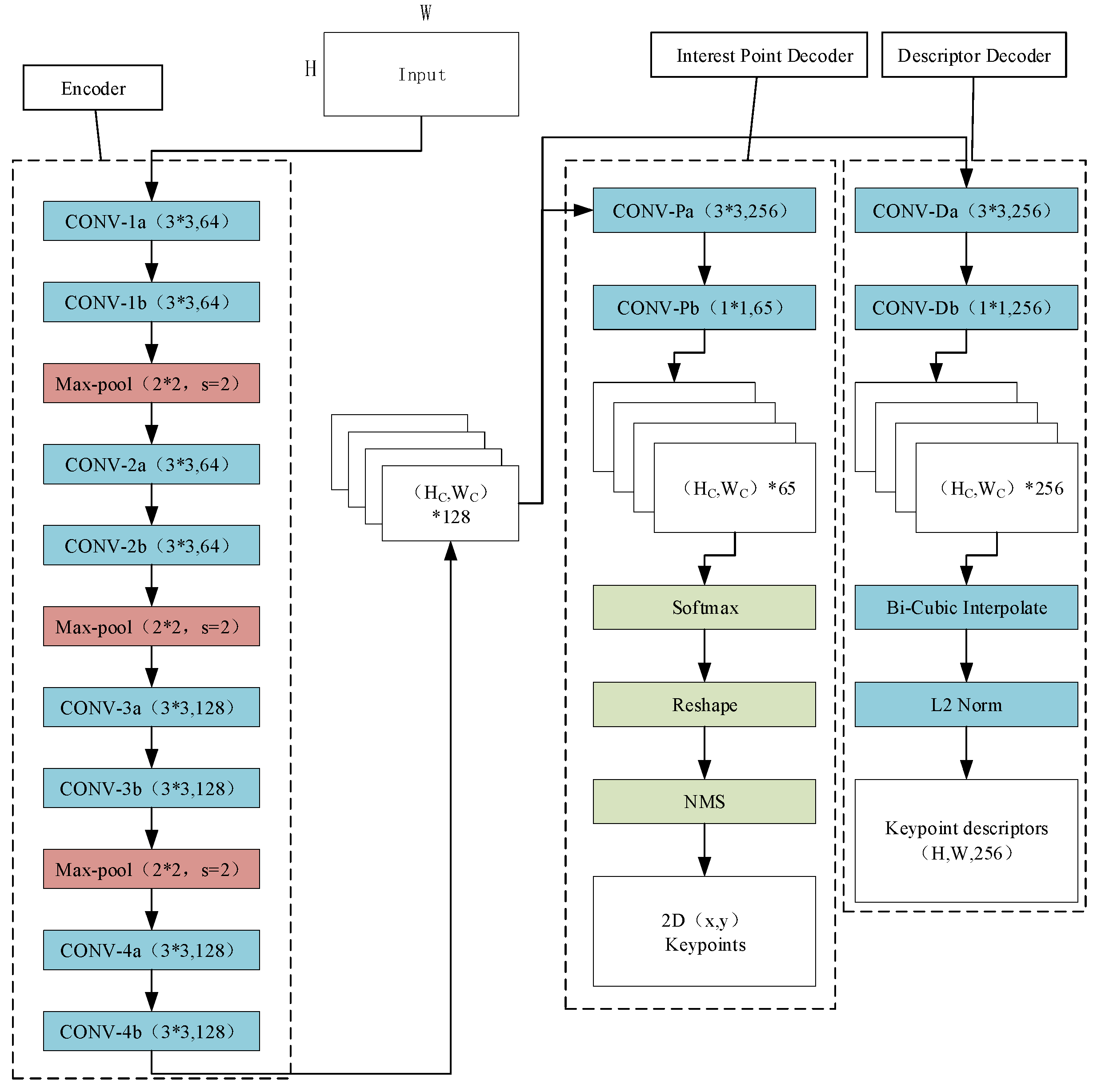
The SuperPoint algorithm is trained using a self-supervised learning approach, eliminating the need for manual annotation of keypoints in images or the manual design of keypoints and descriptors. As shown in Figure 1, its network architecture consists of two main components:

Figure 1.
SuperPoint architecture diagram.
An encoder network adapted from VGG-style architecture, with modifications and adjustments tailored for feature extraction.
Two decoder networks: a keypoint detection decoder and a keypoint descriptor decoder. Since both decoder networks share the aforementioned encoder network, this design ensures a high degree of feature consistency—a critical advantage of the SuperPoint algorithm. By integrating the encoder–decoder structure, the algorithm efficiently generates keypoints and their corresponding descriptors in a unified framework, avoiding the inconsistencies that may arise from using separate networks for detection and description.
- (1)
- Shared encoding layers
The encoding layers primarily consist of a Rectified Linear Unit (ReLU), convolutional layers (Conv), and max-pooling layers (Max-pool). As shown in Figure 1, two convolutional layers and one pooling layer can be regarded as a single block, where the pooling layer has a stride s = 2, and the last block does not include a pooling layer. Therefore, when an image with dimensions (H, W) is input, after processing by the encoding layers, it outputs a tensor of shape (HC, WC, 128). The specific transformation relationship of the image is described by Equation (1):
In the equation, I represents the original image; β denotes the encoded image; and H and W are the height and width of the original image, respectively. HC (encoded image height) and WC (encoded image width) are given by HC = H/8 and WC = W/8.
- (2)
- Interest Point Decoder
After obtaining the tensor of shape (HC, WC, 128) from the shared encoding layers, the next step is to feed it into the keypoint detection decoder network. This tensor first passes through two convolutional layers, transforming it into a tensor of shape (HC, WC, 65). Here, the value 65 corresponds to the local region size of the original image (8 × 8 = 64 positions) plus one additional channel for the non-keypoint class, totaling 65 channels. A softmax operation is then applied to each spatial location across the 65 channels to convert logits into probabilities, after which the non-keypoint class channel is removed. Finally, a reshape operation is performed on the tensor to obtain a new tensor with the size (HC × WC, 64).
- (3)
- Descriptor Decoder
In the decoder network for feature point descriptors, it shares the output of the Encoder’s shared encoding layer with the Interest Point Decoder feature point decoding network. First, it passes through two convolutional layers to transform it into a tensor of size (HC, WC, 256). Then, its size is enlarged through bicubic interpolation. Finally, L2 normalization is performed on each pixel to obtain the descriptors of the image.
2.2. Experimental Environment and Model Evaluation Metrics
The specific experimental environment for this study is presented in Table 1:

Table 1.
Environment configuration.
In this section of the experiment, the operating system used is Windows 11, version 24H2. The programming language is Python 3.9.6, the Deep Learning framework is PyTorch 2.1.0, and the GPU programming interface is CUDA 12.1. The hardware platform for this experiment consists of a 12th Gen Intel(R) Core(TM) i5-12490F 3.00 GHz CPU, an NVIDIA GeForce RTX 3060 (12 GB), and 16 GB of memory.
The evaluation metrics mainly used in this experiment include: the number of feature points, the repeatability of feature points, the calculation speed, and the positioning error. The specific definitions of these metrics are as follows:
Number of Feature Points: This refers to the quantity of image feature points detected by the algorithm during the feature extraction process. If too many feature points are extracted, the model efficiency will be low and there will be a large number of invalid feature points, which is not conducive to subsequent matching. If too few feature points are extracted, it is easy to miss key feature points. There is no fixed standard for the number when comparing different images. Therefore, we cannot simply judge the quality of the model based on this metric alone. We need to combine it with the effect diagram of feature extraction, and it is better that the feature points are sparsely and evenly distributed [9].
Repeatability of Feature Points: This is the proportion of repeatedly detected feature points to the total number of feature points when the illumination or viewing angle of the same image changes. It reflects the robustness and generalization ability of the feature extraction algorithm. The higher this value is, the better the stability and robustness of the corresponding feature extraction algorithm are [10].
Time: This refers to the time required for the feature extraction algorithm to complete the detection for each image. It reflects the performance and execution efficiency of the feature extraction algorithm. The smaller this value is, the higher the model efficiency is [11].
Positioning Error: This is the error between the position of the feature points detected by the feature extraction algorithm and the position of the feature points in the real scene. It reflects the accuracy of the algorithm. The smaller this value is, the better the accuracy of the algorithm is.
2.3. Arison and Analysis of Experimental Results
In this section, several widely used and high-performance feature extraction methods are selected for comparison with the SuperPoint algorithm, including classic traditional approaches such as BRISK, ORB, SIFT and FAST. The dataset used in this experiment is the steel plant dataset. The steel plant image dataset comprises approximately 2000 high-resolution images (resolution: 1920 × 1080) captured across diverse operational zones of a steel mill, including blast furnaces, rolling mills, and material storage areas. The dataset exhibits multi-scenario characteristics, covering normal production states (e.g., stable steel rolling processes and conveyor belt operations), anomalous conditions (e.g., equipment overheating, material blockages, and pipeline leaks), and environmental variations (day/night lighting, dust density, and steam interference). Spatially, the dataset includes both overhead perspective (via fixed industrial cameras) and close-range views (via mobile inspection robots), capturing multi-scale details from macro-process flows to micro-component textures. Temporally, it spans continuous shooting over 12 months, reflecting seasonal operational changes.
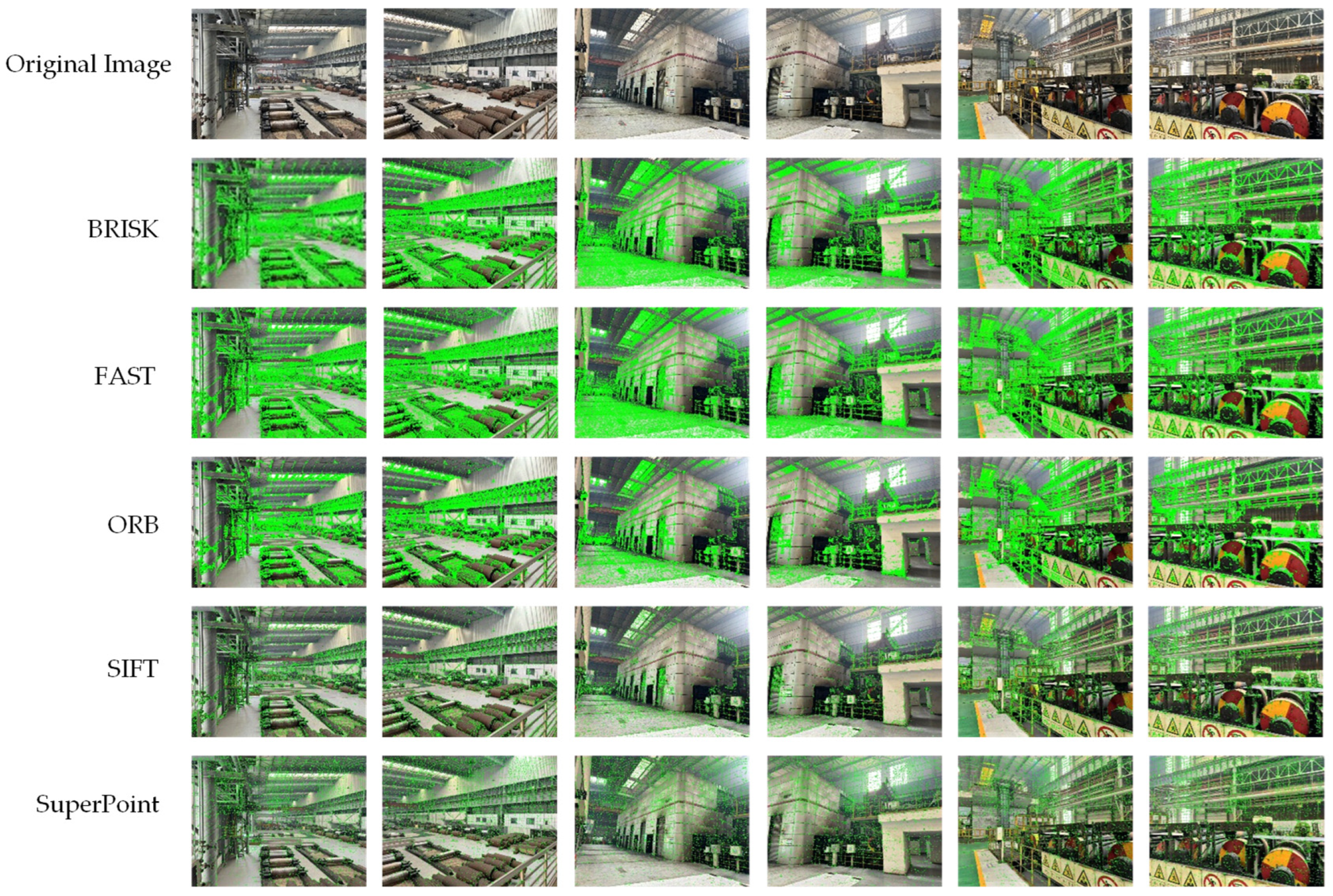
Three sets of stitching-ready images (6 images in total) from different scenes in a steel plant are chosen to demonstrate the specific effects of different feature extraction algorithms. The feature extraction results of these algorithms are shown in Figure 2.

Figure 2.
Feature extraction algorithms comparison.
In Figure 2, it can be observed that traditional algorithms extract an excessive number of keypoints, including a large proportion of invalid ones. This not only increases model computation time but also significantly hinders the real-time requirements for video image stitching.
By conducting experiments on multiple different images using the aforementioned feature extraction algorithms and applying the model evaluation metrics described earlier, the specific algorithm assessment results are summarized in Table 2:
Table 2.
Evaluation results of feature extraction algorithms.
As shown in Table 2, compared with traditional algorithms, the proposed algorithm extracts a relatively small number of keypoints. Combined with the specific feature extraction results in Figure 2, the algorithm achieves comprehensive yet sparse keypoint extraction, which is conducive to the subsequent feature matching process. Additionally, the keypoint repeatability of the proposed algorithm is the highest among all compared methods, reflecting its excellent performance and robustness.
In terms of computational speed, the proposed algorithm is only slightly inferior to the FAST algorithm (renowned for its speed) but significantly outperforms other traditional algorithms. Regarding localization error, while it is slightly less accurate than the SIFT algorithm, it still outperforms all other methods.
Overall, the proposed algorithm demonstrates superior performance in terms of speed, accuracy, and robustness compared to traditional algorithms, laying a solid foundation for subsequent feature matching tasks.
3. Image Feature Matching Based on the Improved LightGlue Algorithm
Through the work in the previous section, this paper has successfully completed the extraction of video image feature points based on the SuperPoint algorithm. The final output results are the corresponding position coordinates of the feature points and the feature descriptor vectors. The next step is to complete the matching of the feature points based on these feature point positions and descriptor vectors, thus laying a solid foundation for the final image fusion. According to Table 2, the number of feature points extracted by the feature extraction algorithm is in the thousands. Facing such a large-scale number of feature points, there must be many invalid feature points, and there will also be a large number of mismatched points during the matching process.
Therefore, based on the above problems, this paper selects the LightGlue algorithm as the matching algorithm. The LightGlue algorithm is a lightweight feature matching algorithm proposed by Philipp Lindenberger et al. in 2023 [8]. It can handle the matching tasks with sparse features very well. At the same time, through its attention mechanism and adaptive inference strategy, it can balance both speed and accuracy.
Moreover, this section also proposes using Agglomerative Clustering (AGG) as a pre-module for LightGlue matching. By clustering the feature points in advance, the matching efficiency and quality can be improved. Finally, in this section, the RANSAC algorithm is added after LightGlue to eliminate mismatched points and improve matching accuracy and quality.
3.1. Basic Principles of the LightGlue Algorithm
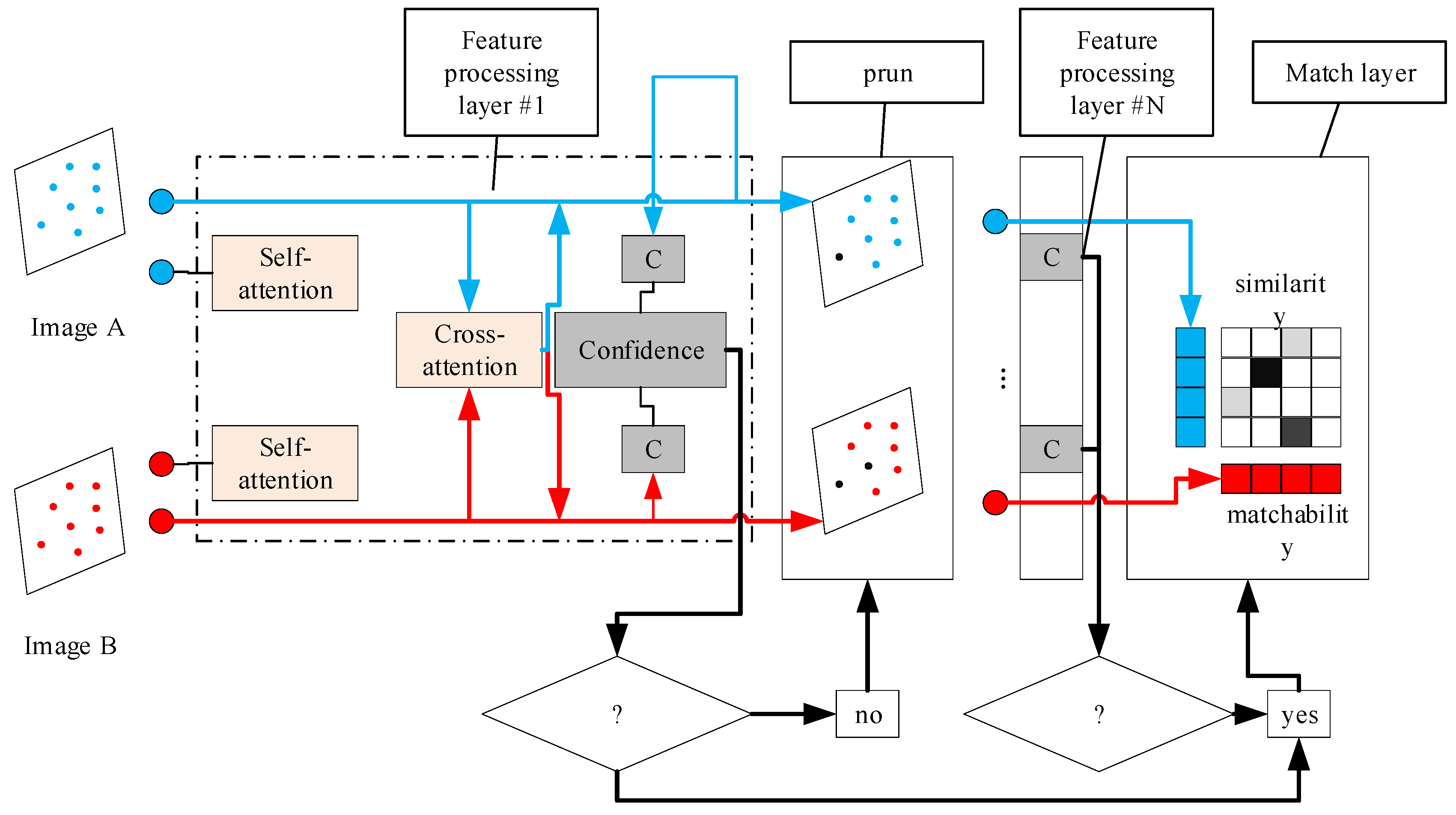
The LightGlue algorithm is derived from the Transformer attention model, and its network structure is shown in Figure 3. It is mainly divided into three parts: The first part is the feature processing layer composed of the self-attention mechanism and the cross-attention mechanism, with a total of N layers. The second part is the confidence judgment layer, which follows the feature processing layer and is mainly responsible for determining whether to exit the iteration of the feature processing layer. The third part is the feature matching layer, which calculates the matching matrix through a lightweight detection head and outputs the matching relationships of the feature points. The following will further introduce the network structure and principle of the LightGlue algorithm through the specific process of feature matching.

Figure 3.
LightGlue architecture diagram.
The LightGlue algorithm starts to work by taking a pair of input feature point position coordinates and feature descriptor vectors (that is, the output of SuperPoint mentioned in Figure 2) as the input. The feature processing layer processes the feature information through contextual content based on the self-attention and cross-attention units. Among them, the feature point descriptor matrices of the images A and B to be matched are:
In the formula, N and M represent the number of feature points in image A and image B, respectively, and C represents the feature dimension. For SuperPoint, C = 256.
Taking XA as an example, the above matrix XA representing the state of feature points generates a query vector QA, a key vector KA, and a value vector VA after linear transformation. Therefore, for a single feature point state xi in image A, it will also be transformed into a query vector qi, a key vector qi, and a value vector qi accordingly. Then, for the query vector qi of each feature point, calculate its similarity with the key vector kj of other feature points, and obtain the weight through softmax normalization as follows:
In the formula, d is the dimension of the attention head; then the weight matrix represents the dependency relationship between feature points.
Finally, the self-attention output X′ is obtained by weighted summation of the value vector VA using the weights, as follows:
This output integrates the information of the current feature point with that of all other feature points, significantly enhancing the connections between features within the same image.
The principle of the cross-attention mechanism is similar to that of the self-attention unit. The only difference is that the query vector comes from image A, while the key vector and the value vector come from image B. Through the cross-attention mechanism, the feature points of one image can focus on all the feature points of the other image. At the same time, this is also the core mechanism of the LightGlue network.
After the feature information is processed by the self-attention mechanism and the cross-attention mechanism, LightGlue performs a confidence judgment. If the confidence judgment layer network determines that the number of feature points with high confidence is small and does not reach the preset threshold, it will continue the next iteration of feature inference, repeating the above-mentioned working process of the self-attention and cross-attention mechanisms. At the same time, a feature point pruning operation will be carried out to remove the feature points with very low confidence. The confidence judgment layer can improve the computational efficiency of LightGlue while ensuring its accuracy. As the feature inference layer iterates continuously, when the confidence judgment network determines in a certain iteration that the number of feature points with high confidence has met the threshold, it will enter the feature matching layer. First, the matching score matrix M is calculated using the features obtained from the above-mentioned iterations:
In the formula, N represents the number of feature points in image A; M represents the number of feature points in image B; represents the similarity score between the i-th point of image A and the j-th point of image B.
Finally, through the matching score matrix and the matchability scores, the LightGlue network will calculate the optimal matches and then output the matching relationships between the two images.
3.2. Agglomerative–LightGlue Feature Matching Model
The Agglomerative Clustering algorithm is an unsupervised machine learning method [12]. The Agglomerative hierarchical clustering algorithm is a bottom-up clustering algorithm. It first treats each data point as a separate cluster. Then, based on specific distance measurement methods such as single-linkage, complete-linkage, or average-linkage, it calculates the distances between clusters. After that, it finds the two closest clusters and merges them into a new cluster. This operation of calculating the distances between clusters and merging them is repeatedly carried out until a preset stopping condition is met, such as reaching a specified number of clusters or a threshold value for the distance between clusters. Eventually, a hierarchical clustering result is formed.
In this section, the idea of Agglomerative hierarchical clustering is considered to optimize the LightGlue algorithm. It mainly involves clustering the output feature points of SuperPoint, and then the LightGlue algorithm performs feature point matching within the same cluster. The specific method is as follows:
Before LightGlue matching, considering the relationship between the two photos, the Agglomerative hierarchical clustering algorithm is used to divide the clusters of the two images simultaneously, reducing the number of regions to be matched. The input part of the Agglomerative Clustering algorithm consists of two parts. The first part is the difference in image positions. The coordinates in the two images are processed for relative position normalization respectively and then input into the clustering algorithm.
The spatial relationship is quantified by the difference in image positions, which captures the relative geometry between camera viewpoints. First, image coordinates are normalized using the steel plant’s layout. For image A and B, their absolute position differences are shown in the following equation:
Normalize the absolute position difference to obtain the normalized difference as (Δx′, Δy′). The definition of the spatial proximity metric is as follows:
If dspatial ≤ 0.05, the images are clustered into one category to ensure that only spatially adjacent images are grouped for matching.
The second part is the pixel difference, and the values of the three RGB elements of the images are input.
The pixel-wise relationship is measured by the pixel difference, which evaluates RGB intensity consistency between images. For each image, the mean (μR, μG, μB) and standard deviation (σR, σG, σB) of pixel values are computed. The photometric distance is derived from normalized pixel differences:
Images with dphoto < 0.3 are clustered, as their pixel distributions (e.g., mean intensities and contrast) are sufficiently similar to enable reliable feature matching.
After integrating the above two inputs, the feature points extracted by SuperPoint are clustered, and the LightGlue matching is carried out for the feature points belonging to the same cluster in the two images. In this way, the number of matches that each feature point needs to calculate is reduced, the matching time consumption is decreased, and the matching efficiency is improved.
To reduce computational complexity, the matching process is constrained within clusters through the following steps: For the hierarchical clustering workflow, the combined feature vector (dspatial, dphoto) for each image pair is fed into an Agglomerative Clustering algorithm with complete linkage (maximizing inter-cluster distances) to form clusters. The algorithm iteratively merges image pairs until the number of clusters K satisfies K ≤ √N (where N is the total number of images), empirically reducing the search space by 60–70%. Within each cluster, SuperPoint keypoints undergo spatial consistency filtering: keypoints with reprojection errors > 3 pixels (estimated via prior camera calibration) are discarded. LightGlue matching is then applied only to keypoint pairs within the same cluster, reducing the number of candidate matches from O(N2) to O(K ∙ M2), where M is the average number of images per cluster.
RANSAC (Random Sample Consensus) is an iterative algorithm for robustly estimating the parameters of a mathematical model from data containing outliers, which is widely used in fields such as computer vision and robotics. Its core idea is to randomly select a minimum sample subset (for example, select two points to fit a straight line) to fit the model, calculate the errors between all data points and the model to distinguish inliers (valid data conforming to the model) and outliers (abnormal data), and through multiple repeated iterations, the model with the most inliers is retained as the optimal solution.
After the image feature matching is completed by the above image matching algorithm based on Agglomerative + LightGlue, the RANSAC algorithm is integrated in this section to remove the mismatched points, further improving the accuracy of image stitching.
3.3. Comparison and Analysis of Experimental Results
In this section of the experiment, two evaluation indicators are selected: the matching accuracy rate and the matching time. The specific definitions of the indicators are as follows:
Matching Accuracy Rate (Accuracy): The matching accuracy rate refers to the proportion of the number of correctly matched point pairs to the total number of matched point pairs. It reflects the accuracy of the feature matching algorithm. The larger this value is, the better the accuracy of the corresponding feature matching algorithm is, and the better its performance is [13].
Matching Time (Time): The matching time refers to the time required for the feature matching algorithm to complete matching for each group of images to be stitched. It reflects the performance and work efficiency of the feature matching algorithm. The smaller this value is, the better the performance of the corresponding feature matching algorithm is [14].
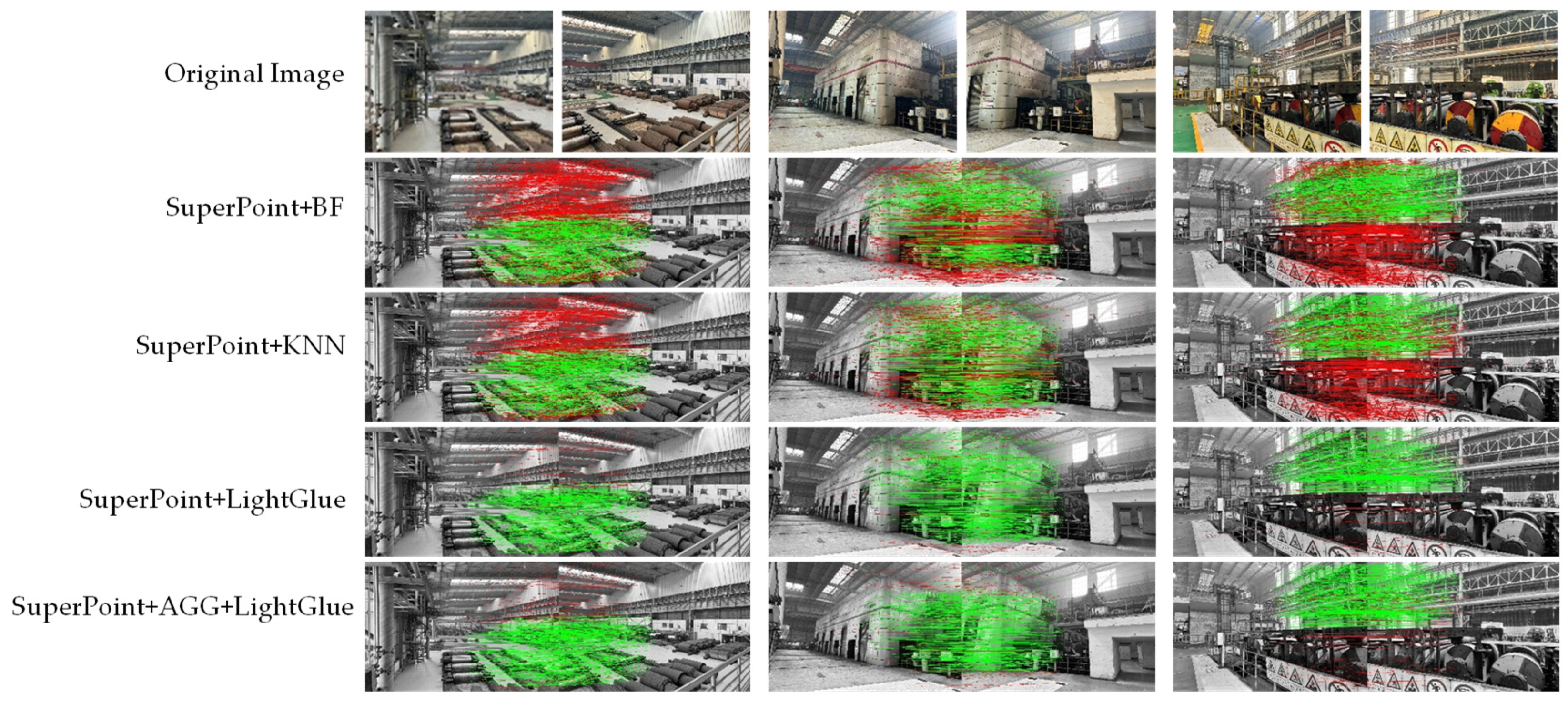
On the basis of having already completed the feature extraction by SuperPoint in the previous text, in order to verify the effectiveness of the algorithm in this section, four groups of control experiments are set up, which are as follows: SuperPoint + AGG + LightGlue (the algorithm of this chapter), SuperPoint + LightGlue, and SuperPoint + KNN. Comparison with SuperPoint + LightGlue can verify the performance improvement of the algorithm in this section after the improvement, while comparison with SuperPoint + KNN can verify that the LightGlue algorithm is superior to the traditional algorithm. The experimental results are shown in Figure 4.

Figure 4.
Feature matching comparison results.
In Figure 4, BF (Brute Force) refers to the brute-force matching algorithm; KNNKNN refers to the k-nearest neighbors algorithm, both of which are typical and commonly used image matching algorithms. In Figure 4, the green matching lines represent the correctly matched feature points, and the red connection lines represent the incorrectly matched feature points. It can be clearly seen from Figure 4 that the correct matching rate of the LightGlue algorithm is significantly better than that of the other methods.
At the same time, combined with the above-mentioned evaluation indicators, the specific algorithm evaluation results shown in Table 3 can be obtained.
Table 3.
Experimental data comparison.
As shown in Table 3, compared with traditional methods, the LightGlue algorithm greatly improved the matching accuracy rate. However, it is somewhat behind traditional methods in terms of matching speed. Through analysis, it is likely that this is caused by setting up many feature point detection layers during the training process in order to place a greater emphasis on accuracy. After the improvement of the algorithm in this section, it can be seen that on the basis of maintaining the matching accuracy rate, the matching time has been reduced by 26.2%. In summary, the algorithm presented in this section performs better than other algorithms in terms of both matching time and matching accuracy rate. It has relatively high real-time performance and accuracy in stitching, providing excellent preparatory conditions for subsequent video image fusion.
4. Image Fusion Improved Based on Dynamic Pixel Adaptability
After completing the image feature matching, if the image fusion is carried out directly, due to the influence of factors such as the perspective differences between different images and matching errors, the final stitched image may have quality defects. A suitable image fusion algorithm can, to a certain extent, eliminate the influence of these defects, thereby improving the final stitching quality.
However, traditional image fusion algorithms usually still have the problems of perspective flattening and ghosting. In response to this situation, this paper proposes a general dynamic adaptive fusion strategy to solve the problems of perspective flattening and ghosting in the overlapping areas.
4.1. Basic Principle of Fade-In and Fade-Out Weighted Fusion
The fade-in and fade-out weighted fusion algorithm is a commonly used technique for handling overlapping regions in image stitching. By assigning gradient weights to different images in the overlapping region, it achieves a natural transition to eliminate stitching marks [15]. Its core function is to perform a weighted sum of the pixels in the overlapping region. For example, a decreasing weight from 1 to 0 is assigned to the left image, and an increasing weight from 0 to 1 is assigned to the right image. Weight functions include forms such as linear (for example, changing linearly with the distance from the boundary) and Gaussian (generating smooth weights through a Gaussian kernel), which make the fusion boundary smooth. The specific steps are as follows: first, determine the overlapping region, then generate the corresponding weight map, and finally, fuse the pixels according to the weights. The pixel value of the fused image region is as follows:
In the formula, represents the fused pixel value; , respectively, represent the pixel values of the images to be stitched at the coordinates ; is the weight of the corresponding pixel; and .
4.2. Dynamic Adaptive Fusion Strategy of Pixels
In the geometric alignment stage, to address the stitching scene tasks with parallax, instead of using the global homography matrix strategy used in traditional solutions, a strategy of using homography matrix transformation in the overlapping area according to the specific perspective position is proposed. The specific steps are as follows: First, divide the images to be stitched into multiple sub-regions with overlapping parts. This division is crucial as different regions may have distinct geometric characteristics due to parallax. For example, in a panoramic image stitching scenario where the camera rotates around a vertical axis, the upper and lower parts of the images may have different degrees of distortion. By partitioning the images, we can handle these differences more effectively.
Then, calculate the corresponding homography transformation matrices for different regions. To calculate the homography matrix for a sub-region, we first identify a set of corresponding feature points in the overlapping parts of the sub-regions from different images. Once the corresponding feature points are obtained, the homography matrices for different regions are calculated through the RANSAC algorithm.
Next, complete the geometric alignment and projection transformation of each sub-region according to the corresponding homography transformation matrix. When performing the projection transformation, we apply the calculated homography matrix to each pixel in the sub-region. For a pixel with coordinates (x, y) in one image, the transformed coordinates (x′, y′) in the stitched image can be obtained through matrix multiplication:
In the formula, H represents the homography matrix.
In this way, the parallax problem caused by the traditional globally consistent homography matrix can be effectively solved.
In the image fusion stage, based on the pixel difference value, an improved fusion scheme based on pixel difference is proposed. Align the overlapping areas through the homography matrix but avoid global unified projection and retain the original perspective of the non-overlapping areas. This approach ensures that the natural appearance of the non-overlapping parts of the images is maintained, which is important for preserving the overall visual integrity of the stitched image.
Then, establish a difference response mechanism through pixel difference analysis; calculate the chromaticity space difference value of the two images (such as the Euclidean distance of the three RGB channels) for each overlapping pixel point. For an overlapping pixel with RGB values (R1, G1, B1) in one image and (R2, G2, B2) in the other image, the Euclidean distance is then calculated as
When the difference value is less than the preset threshold, use the fade-in and fade-out weighted fusion algorithm to determine the fused pixel value.
When the difference value exceeds the threshold, start the neighborhood consistency verification mechanism: construct a 3 × 3 neighborhood window centered on the target pixel and calculate the gradient structure similarity index of the two images within this area. To calculate the gradient structure similarity index, we first calculate the gradients of the images in the neighborhood. For an image I (x, y), the gradients in the x and y directions can be calculated using operators like the Sobel operator. The Sobel operator in the x direction is and in the y direction is . After obtaining the gradients, we compare the structures of the gradients in the two images within the 3 × 3 neighborhood. We preferentially select the pixel of the source image with higher local feature consistency as the fusion output. This process ensures that the fused image has consistent local features and reduces the appearance of artifacts caused by large differences between the source images.
By adopting the local homography matrix and the pixel adaptive fusion mechanism, this scheme can effectively solve the parallax problem and the ghosting problem in the image fusion process, successfully improve the final video image stitching quality, and achieve global smooth stitching.
4.3. Comparison and Analysis of Experimental Results
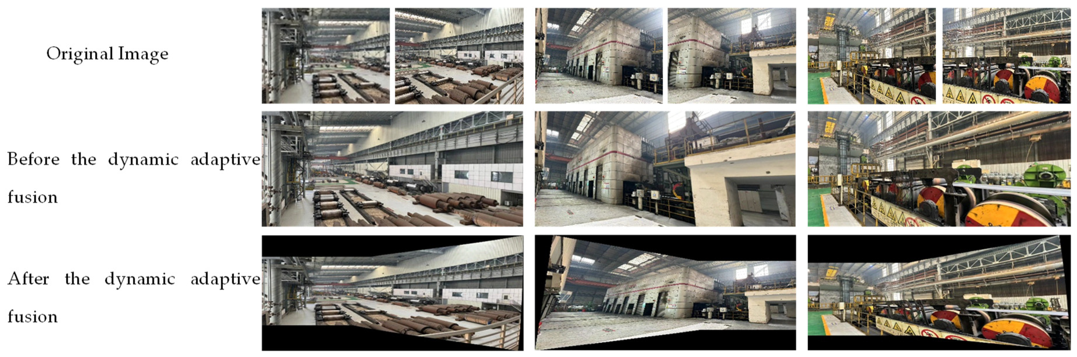
On the basis of the fade-in and fade-out weighted fusion algorithm, combined with the improvement and optimization of the dynamic adaptive fusion strategy mentioned above, three groups of images mentioned previously are selected for experimental comparative analysis in different scenarios. The final stitched images after image fusion are shown in Figure 5:
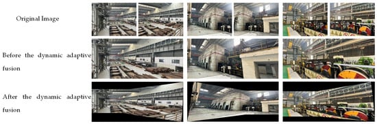
Figure 5.
Effects of dynamic adaptive pixel fusion strategy.
As shown in Figure 5, before the improvement of dynamic adaptive fusion, due to the fact that the fade-in and fade-out weighted fusion algorithm uses a global homography transformation matrix, the overall stitching result presents a flattened perspective and the spatial effect is relatively poor. At the same time, there are also stitching quality problems such as ghosting in the image stitching effect. However, after applying the improved algorithm in this section, the overall stitched image presents a spatial perspective consistent with the shooting angle, and problems such as ghosting after stitching have also been solved.
5. Conclusions
First of all, this paper adopts the SuperPoint algorithm as the feature extraction algorithm. The experimental results show that this algorithm is superior to traditional algorithms in both the speed of feature extraction and the accuracy of extraction. Then, the LightGlue algorithm is selected as the feature matching algorithm, and it is optimized and improved by combining it with the Agglomerative hierarchical clustering algorithm. The experimental results show that this improvement effectively improves the speed of feature matching. Compared with the original LightGlue algorithm, the matching efficiency is increased by 26.2%. Finally, aiming at the problems of parallax and ghosting existing in the image fusion process, this solution proposes a dynamic adaptive fusion strategy of pixels, and makes improvements and optimizations in both the geometric alignment and pixel fusion processes. The experimental results show that this improvement successfully solves the problems of parallax and ghosting and achieves a good image stitching effect.
Although this study achieves effective industrial image stitching via the dynamic adaptive fusion strategy, it faces two primary limitations: high hardware cost requirements due to the computational intensity of the SuperPoint + LightGlue framework, and limited generalizability across diverse environments (e.g., drastic lighting changes or varying industrial textures). For future work, we aim to further explore model lightweighting techniques (such as knowledge distillation and neural architecture search) to reduce computational complexity, making the algorithm deployable on low-cost edge devices, and enhance the model’s environmental robustness through domain adaptation strategies (e.g., training on synthetic datasets with simulated lighting/noise variations) to extend its applicability to broader industrial scenarios, including outdoor steel yards and high-dust workshops. These efforts will address the current hardware and generalizability constraints, promoting wider industrial adoption of the stitching solution.
Author Contributions
Conceptualization, Y.F. and F.Z.; methodology, Y.F.; software, Y.F.; validation, Y.F., X.L. and F.Z.; formal analysis, F.Z.; investigation, Y.F. and F.Z.; resources, F.Z., X.X. (Xiaofei Xiang) and L.W.; data curation, X.X. (Xiong Xiao) and X.L.; writing—original draft preparation, Y.F. and F.Z.; writing—review and editing, Y.F. and F.Z.; visualization, X.L.; supervision, X.X. (Xiong Xiao); project administration, F.Z.; funding acquisition, F.Z., X.X. (Xiaofei Xiang) and L.W. All authors have read and agreed to the published version of the manuscript.
Funding
This research was funded by the National Key Research and Development Program of China, grant number 2022YFB3304000.
Data Availability Statement
The datasets presented in this article are not readily available because the data are part of an ongoing study. Requests to access the datasets should be directed to yuening_4012@foxmail.com.
Acknowledgments
I would like to express my deepest gratitude to my family for their unwavering love, understanding, and support throughout my research journey. Their encouragement has been my constant source of strength. I am also immensely thankful to the University of Science and Technology Beijing for providing an excellent academic environment, valuable resources, and professional guidance, which have been instrumental in the completion of this work.
Conflicts of Interest
The authors declare no conflicts of interest.
References
- Kuglin, C.D. The phase correlation image alignment method. In Proceedings of the International Conference on Cybernetics and Society, San Francisco, CA, USA, 23–25 September 1975; pp. 163–165. [Google Scholar]
- Brown, M.; Lowe, D.G. Recognising panoramas. In Proceedings of the Ninth IEEE International Conference on Computer Vision, Nice, France, 14–17 October 2003; pp. 1218–1225. [Google Scholar] [CrossRef]
- Bay, H.; Tuytelaars, T.; Van, G.L. Surf: Speeded up robust features. In Proceedings of the Ninth European Conference on Computer Vision, Graz, Austria, 7–13 May 2006; pp. 404–417. [Google Scholar] [CrossRef]
- Rublee, E.; Rabaud, V.; Konolige, K.; Bradski, G. ORB: An efficient alternative to SIFT or SURF. In Proceedings of the 2011 International Conference on Computer Vision, Barcelona, Spain, 6–13 November 2011; pp. 2564–2571. [Google Scholar] [CrossRef]
- DeTone, D.; Malisiewicz, T.; Rabinovich, A. Superpoint: Self-supervised interest point detection and description. In Proceedings of the IEEE Conference on Computer Vision and Pattern Recognition Workshops, Salt Lake City, UT, USA, 18–22 June 2018; pp. 224–236. [Google Scholar] [CrossRef]
- Tyszkiewicz, M.; Fua, P.; Trulls, E. DISK: Learning local features with policy gradient. Adv. Neural Inf. Process. Syst. 2020, 33, 14254–14265. [Google Scholar]
- Sarlin, P.E.; DeTone, D.; Malisiewicz, T.; Rabinovich, A. Superglue: Learning feature matching with graph neural networks. In Proceedings of the 2020 IEEE/CVF Conference on Computer Vision and Pattern Recognition, Seattle, WA, USA, 13–19 June 2020; pp. 4938–4947. [Google Scholar] [CrossRef]
- Lindenberger, P.; Sarlin, P.E.; Pollefeys, M. Lightglue: Local feature matching at light speed. In Proceedings of the IEEE/CVF International Conference on Computer Vision, Paris, France, 4–6 October 2023; pp. 17627–17638. [Google Scholar] [CrossRef]
- Borman, R.I.; Harjoko, A. Improved ORB Algorithm Through Feature Point Optimization and Gaussian Pyramid. Int. J. Adv. Comput. Sci. Appl. 2024, 15, 268–269. [Google Scholar] [CrossRef]
- Kusnadi, A.; Winantyo, R.; Pane, I.Z. Evaluation of Feature Detectors on Repeatability Quality of Facial Keypoints In Triangulation Method. In Proceedings of the 2018 International Conference on Smart Computing and Electronic Enterprise (ICSCEE), Shah Alam, Malaysia, 11–12 July 2020; Volume 21, Issue 2. pp. 150–156. [Google Scholar] [CrossRef]
- Lee, J.; An, H.M.; Kim, J. Implementation of the high-speed feature extraction algorithm based on energy efficient threshold value selection. Trans. Electr. Electron. Mater. 2020, 21, 150–156. [Google Scholar] [CrossRef]
- Durante, F.; Gatto, A.; Saminger-Platz, S. On Agglomerative Hierarchical Percentile Clustering. In Proceedings of the 19th World Congress of the International Fuzzy Systems Association (IFSA), Bratislava, Slovakia, 19–24 September 2021; pp. 616–623. [Google Scholar] [CrossRef]
- Canaz Sevgen, S.; Karsli, F. An improved RANSAC algorithm for extracting roof planes from airborne lidar data. Photogramm. Rec. 2020, 35, 40–57. [Google Scholar] [CrossRef]
- Yang, Q.; Qiu, C.; Wu, L.; Chen, J. Image matching algorithm based on improved fast and ransac. In Proceedings of the 2021 IEEE International Conference on Mechatronics and Automation (ICMA), Takamatsu, Japan, 8–11 August 2021; pp. 142–147. [Google Scholar] [CrossRef]
- Shen, J.; Qian, F.; Chen, X. Multi-camera panoramic stitching with real-time chromatic aberration correction. J. Phys. Conf. Ser. 2020, 1617, 012046. [Google Scholar] [CrossRef]
Disclaimer/Publisher’s Note: The statements, opinions and data contained in all publications are solely those of the individual author(s) and contributor(s) and not of MDPI and/or the editor(s). MDPI and/or the editor(s) disclaim responsibility for any injury to people or property resulting from any ideas, methods, instructions or products referred to in the content. |
© 2025 by the authors. Licensee MDPI, Basel, Switzerland. This article is an open access article distributed under the terms and conditions of the Creative Commons Attribution (CC BY) license (https://creativecommons.org/licenses/by/4.0/).