Posture and Map Restoration in SLAM Using Trajectory Information

Abstract

SLAM algorithms generally use the last system posture to estimate its current posture. Errors in the previous estimations can build up and cause significant drift accumulation. This accumulation of error leads to the bias of choosing accuracy over robustness. On the contrary, sensors like GPS do not accumulate errors. But the noise distribution in the readings makes it difficult to apply in high-frequency SLAM systems. This paper presents an approach which uses the advantage of both tightly-coupled SLAM systems and highly robust absolute positioning systems to improve the robustness and accuracy of a SLAM process. The proposed method uses a spare reference trajectory frame to measure the trajectory of the targeted robotic system and use it to recover the system posture during the mapping process. This helps the robotic system to reduce its accumulated error and able the system to recover from major mapping failures. While the correction process happens whenever a gap is detected between the two trajectories, the external frame does not have to be always available. The correction process is only triggered when the spare trajectory sensors can communicate. Thus, it reduces the needed computational power and complexity. To further evaluate the proposed method, the algorithm was assessed in two field tests and a public dataset. We have demonstrated that the proposed algorithm has the ability to be adapted into different SLAM approaches with various map representations. To share our findings, the software constructed for this project is open-sourced on Github.

1. Introduction

Simultaneous Localization and Mapping (SLAM) is a growing technology that is utilized in Robotics, Unmanned Aerial Vehicle (UAV), Augmented Reality/Virtual Reality (AR/VR), Autonomous Vehicle (AV), etc. and it is implemented for the end users within industries such as Military, Agriculture & Forestry, Mining, Automotive, Manufacturing & Logistics, Household Appliance, and many more [1,2].

The SLAM technology is used in UAVs [3] as an essential tool for navigation, flight control, and collision avoidance. In addition, it is used in a variety of robots in manufacturing, transport, assembly and packing, earth and space exploration, weaponry, surgery, and laboratory research. Moreover, the Industry 4.0 revolution, going on at full steam, is driving the demand for autonomous mobile industrial robots [4,5], which depend on the SLAM technology to make their way around the factory floor.

SLAM algorithms are widely used in many map construction processes. The scenarios vary from indoor to outdoor with different setups and predominantly contain a camera or Light Detection and Ranging (LiDAR) with inertial odometry. Different approaches can be seen from scanning the layout of streets to mapping the structure of a mining tunnel. As a popular research field, SLAM approaches quickly developed from 2-D occupancy grids to RGB-D maps. While the rapid development of SLAM technology gradually improves the performance of mapping, there are still bottlenecks that create severe degradation in the reliability of a robotic system. One of these bottlenecks is the ability to recover from mapping errors developed through accumulated drifts or rapid environmental changes such as kidnaps and rollovers. During a stable movement, frame-to-frame scan matching algorithms receive minor drifts between each frame. However, any sudden movement will most likely cause the algorithm to lose track.

To partially address the problem, the recent development of Visual Odometry (VO) and SLAM systems adopted the trend of splitting the mapping processes into different levels of mapping frequency and accuracy which are executed in a multi-threaded architecture. This multi-level system uses the strategy of updating the system status in isolated steps:

1.

Local Frame Matching, using the current LiDAR or camera reading to compare with the previous reading and estimate the new system pose based on the previous. This step is often easy to compute but suffers from high drift accumulation.

2.

Local to Submap Matching, taking the current reading and comparing it to a submap. The submap is chosen by a sliding window centered at the current system pose. This step greatly reduces the drift accumulation but is limited by its computational complexity.

The combination of these layers requires the LiDAR or camera to sample the environment as frequently as possible to maintain low drifts, which subsequently requires high computational power. A higher sampling rate will generate a more accurate system orientation as the matching targets are closer to the targets in the previous frame. As a result, Global Navigation Satellite System (GNSS), Ad-Hoc beacons, or other absolute localization techniques are rarely seen in these systems due to their high noise distribution in a short period of time. Additionally, these sensors only provide system pose in 3 degrees-of-freedom (DOF) and do not help to estimate the orientation of the robot by a single reading frame. On the other hand, absolute positioning systems feature high robustness. More importantly, they directly translate the system pose to the global frame. These sensors do not rely on the previous system pose to estimate the current system pose, thus the errors are not accumulative. Combining absolute positioning systems into the SLAM process could improve the robustness of the system and helps the system to overcome significant mapping failures.

There are many studies conducted to address enhancing the robustness and improving the accuracy of SLAM processes. However, to the best of our knowledge, most of these methods emphasize improving accuracy through strengthening sensing power. Though mapping accuracies have been improved via different approaches, the current operational methods suffer drifting cumulation problems. Occupancy grid is a classic method used in earlier SLAM approaches to represent the map. 2-D methods such as Hector SLAM [6], GMapping [7], Cartographer [8] and Karto SLAM [9] scanning matches the environment with an established map to update the grid through linear interpolation. Each grid cell represents the possibility of having obstacles in the area. Since grid cells are the smallest unit on the map, it also indicates the resolution of the map. These methods uses Iterative Closest Point (ICP) [10,11,12] or Normal-Distributions Transform (NDT) [13,14,15] based algorithms to perform scan matching. Due to the nature of grid maps, these algorithms can be easily transformed into 3-D methods [16,17]. However, the computational costs increase as the resolution and map size expand [18]. Furthermore, grid map-based approaches mainly feature navigation and lack details on the map. The information recorded is associated with the resolution of the grid. Lower resolution helps the system to tolerate mapping errors [6]. However, a low-resolution map also provides less information. Upscaling the resolution eventually leads to the trend of directly manipulating point clouds. Moreover, scanning frequency is also an important factor in obtaining high accuracy mapping of an environment. A tightly-coupled LiDAR-Inertial odometry requires both LiDAR and Inertial Measurement Unit (IMU) readings in high frequency [19,20,21].

Other than ICP and NDT-based algorithm families, a method of pose estimation, called LOAM, was created by [22] relying on extracting feature points from selected surfaces. It uses a two-level architecture where a LiDAR reading matches with the previous reading and the constructed map respectively. This multi-level process improves both the updating frequency and the accuracy of the mapping result. This idea was extended by [23] with more detailed feature engineering. A more selective points extraction strategy was integrated into the work which especially suits the application of Unmanned Ground Vehicle (UGV). Zhang and Singh [24] later adopted this method into VO approach and showed a significant improvement in its accuracy. These kinds of multi-level architectures can also be seen in other VO approaches [25,26]. A multi-level scan-matcher significantly reduces the accumulated error by constantly checking the current system pose with the established map. Campos et al. [27] stored submaps in different containers and matches between submaps to perform loop-closing and eliminate potentially damaged mapping results. Loop closing using submaps can be seen in the works shown by [28,29,30]. Time, distance, and landmarks could be used as an indicator to trigger the segmentation. In [31], a new submap is created every 7 m that the robot travels. It is worth mentioning that the submapping in this work also contributes to reducing the impact of long corridors and other featureless scenarios in the mapping results. A similar approach was adopted by [32], but instead of 7 m, the latter creates submaps in every 2.5 m or after a significant rotation. However, in the latter work, not all the submaps were integrated into the global map in the world frame. Discarding low-quality submaps in a matching process helped to keep the accuracy of the results.

Other than improving the scan-matching performance, SLAM also faces challenges from sensor degradation and feature complexity, especially in mixed environment [33]. Since SLAM mainly depends on LiDAR and cameras, modifying the sensing modules directly improves the outcome [34,35,36]. However, a more general solution allows the system to deal with a wider range of scenarios. Early studies uses environment classification to handle environmental complexity [37,38,39]. An artificial neural network (ANN) based classifier was utilized by [40] to evaluate whether the robot is currently in an indoor or outdoor environment. The neural network was trained base on existing data. The system integrated a monocular camera dedicated to classifying the state of the environment. The ANN decided if the robot should rely on a LiDAR-based SLAM system or a stereo camera-based terrain mapping system. A more straightforward approach to distinguish different environments is taking advantage of GNSS sensor signal strength. Dill et al. [41] used the number of satellites a GNSS is communicating with to justify the current situation of the system. A healthy GNSS reading will lead the robot to use Global Positioning System (GPS) and IMU to estimate its pose on the map. In contrast, if GPS lacks satellite connection, then the robot will rely on LiDAR and RGB camera to locate itself. Elevation information could also be used to determine terrain factors during the SLAM process [42]. A combination of a 2-D LiDAR sensor with a DC motor ables the LiDAR to move along Z-axis. The tilt movement of LiDAR gives elevation readings of the obstructions in front of the robot. Based on different elevation readings, the terrain can be classified into the ground, obstacle, and overhanging objects. The classification results further allow the system to decide if it is entering or exiting from an indoor space. In [43], the performance potential of autonomous vehicle sensor systems was assessed to obtain high-definition maps based on several Velodyne sensors as well as a high-performance GNSS/IMU navigation system for creating accurate point clouds. Chiang et al. [44] investigated an integrated design combining inertial navigation system (INS)/GNSS/3D and LiDAR-SLAM in varied environments using a real-world dataset.

Some recent works showed approaches targeting drift accumulation and mapping errors using landmarks and bag-of-words (BoW) methods, regardless of the environment [45]. Using Lisbon Zoo as an example, 3-D LiDAR and cameras were integrated to continuously map a large proportion of the zoo [46]. This work used 3-D LiDAR to map the environment and stores in point clouds. A stereo camera was equipped to take key frames during the operation of the SLAM process. The method extracts BoW features from key frames periodically. Each BoW feature is then stored into a database with pose information recorded at the moment of that frame. Similar in [47,48,49], a matching in BoW from the future key frames will provide the system information to recover from cumulated localization errors. However, both laser and colour based visual navigation systems still suffer from robustness problems. Compare with visual-based sensors, IMUs are less sensitive to the change in environment. Fusing a Magneto-Inertial Measurement Unit (MIMU) with a classic Visual/inertial navigation system (VINS) can significantly improve the error cumulation problem that traditional IMU measurement suffers [50]. In that study, the author applied an inverse square-root filter to the readings from a MIMU and uses it as additional information for system localization. The MIMU enhanced VINS showed better performance in an indoor-outdoor mixed testing environment, especially in poor lighting conditions. It is demonstrated by [51] that real-time kinematic (RTK) and IMU integrated positioning method provided integrated navigation for complex urban environments, and it also provided continuous and reliable high-precision positioning results in weak satellite signal coverage scenarios, such as overhead occlusion, short tunnels, and urban canyons.

SLAM system relies on accurate sensors to incrementally build a map. The trend of acquiring higher resolution maps results in a choice of the more sensitive sensor rather than robustness. While LiDAR offers great accuracy, sensors like GPS and other GNSS could provide a more robust reading in the long run. Thus, a method is required to combine both the accuracy and the robustness from different sensors to not only locate a SLAM system after an interruption but also recover existing mapping errors. In order to solve this problem, this article proposes a spare trajectory correction algorithm based on the integration of a GNSS unit into a SLAM system. The proposed method could help SLAM systems recover from fatal mapping errors and improve the adaptability of the system into more complex working scenarios.

2. Contribution of This Study

In this work, we focused on improving SLAM accuracy and robustness using supplementary trajectory information from an absolute positioning system. We took the concept of the multi-level map updating and discussed the method of using these absolute positioning systems to enhance the accuracy and robustness of current SLAM algorithms. This work is developed based on the concept of trajectory matching [52,53]. We expand the idea from orientation correction to map restoration and attempted to implement the proposed algorithm to different SLAM algorithms to validate its performance. The main contributions of this work are:

• A trajectory matching strategy that combines the advantages of both high-frequency iterative positioning and low accuracy absolute positioning. Other than a frame to frame accuracy, our method seeks to improve the overall mapping accuracy by interpolating the system pose based on readings from a secondary trajectory frame.
• Mapping results correction. Based on the outcome of the trajectory matching process, we took the transform information between the two frames and used it to correct the mapping results. We used a sliding window to control the size of the active area that participates in the correction, thus reducing its computational complexity.
• Loosely-integrated mapping process makes our method insensitive to the environment. While most of the absolute positioning systems, especially GNSS, faces reception problems in mixed environments, our method does not require a continuous trajectory. Instead, the algorithm samples the trajectory received and only outputs estimations when it finds a high-quality match.
• Easily adapted into different SLAM approaches. The proposed method does not affect the main process of SLAM. Instead, it works as an attachment of a targeted SLAM algorithm. We have demonstrated the ability to adopt the proposed method into different SLAM frameworks in the experiments section of this article. The applications vary from 2-D grid map SLAM to 3-D point cloud SLAM. Our study shows that the proposed method significantly improves the quality of the mapping results in all tests.

These contributions make the proposed trajectory matching method significantly more robust than the approaches that are covered in the literature. It also greatly reduces the impact of accumulated drift in a long-term mapping process. The organization of this paper is as follows: Section 1 reviewed some of the existing SLAM approaches and methods of pose and map correction. Section 3 provided a description of the proposed method. Section 4 documented the experiments using the proposed method and evaluated its performance. Finally, Section 5 concluded the feature and performance of the proposed method.

3. Proposed Method

The method proposed in this article aims to fit into an existing SLAM approach and improve its performance over drift accumulation. In this work, we choose Hector SLAM and LOAM as the targeted SLAM algorithms. The proposed Iterative Trajectory Matching (ITM) method requires a minimum of two trajectories. The first one is the trajectory of the SLAM algorithm. Another is the trajectory of a reference frame, such as a GNSS or a laser tracker. The concept of the ITM method is based on the expectation that the reference trajectory has better robustness compare with the SLAM trajectory. It is worth noting that most SLAM algorithms use an initial pose to decide the orientation of their world coordinate system. Our algorithm requires a pre-defined transform from the GNSS frame to local odometry. When the SLAM algorithm performing correctly, the geometrical similarity of the two trajectories could be used to exam the quality of the SLAM process. We monitor the difference between the two using an approach similar to the point-to-point ICP. Once the difference passes a threshold, a matching process will be triggered to align the orientation of the SLAM trajectory according to the reference frame.

Overall, our method uses the Mean Squared Error (MSE) between the two trajectories as the cost function. We use the Levenberg-Marquardt method to convergence the translation and rotation. After that, the results are sent to the SLAM module. Transformation is applied to pose and map respectively in the SLAM module. Figure 1 explains the process of the proposed ITM method using a flow chart. While the ITM module is receiving pose information from both the reference frame and the SLAM frame, the algorithm is executed periodically, based on a timer.

3.1. Trajectory Alignment

The alignment of trajectory orientations is performed using the method developed based on our previous work [52]. Figure 2 shows an example of the trajectory alignment process where the SLAM trajectory is matching the reference trajectory. The ITM outcome is shown in the dashed line which overlapping with the reference trajectory. This indicating a match where the residual of the Levenberg-Marquardt (L-M) method passes the threshold. The rotation and translation are then applied to the SLAM trajectory which results in the pairing of the ITM trajectory and the reference trajectory on the right side of the figure.

The matching between two trajectories can be described by Equation (1), Let L, H be the two sets of coordinates from the trajectories of the reference frame and the SLAM during period T. A downsampling filter is required to ensure both trajectories have same amount of points where $L=\left\{l_1,\dots ,l_n\right\},H=\left\{h_1,\cdots ,h_n\right\}$. The best guess of the initial rotation in quaternion is $w=1,x=0,y=0,z=0$ and translation is $x=0,y=0,z=0$. This is because two trajectories should be close to each other while mapping works correctly.

$$E(q,tr)=\frac{1}{N_l}\sum _{i=1}^{N_l}{∥l_i-q·h_i-tr∥}^2$$

(1)

Using Equation (1) as the cost function, The matching provides a pair of rotation $q^{*}$ and translation $t{r}^{*}$ as the outcome if the L-M method converges with a relatively small residual. To avoid unnecessary correction, $q^{*}$ and $t{r}^{*}$ need to excess a pre-set threshold. Limiting the residual and the transformation is to avoid corrections when the drift is not severe or the match is poor.

Algorithm 1 shows the pseudo-code for the described process. HT here reference to the trajectory generated from Hector SLAM node and RT is the trajectory from the reference frame. In actual coding, the function described here is split into a few functions and placed both inside Hector node and as individual nodes by themselves.

Algorithm 1 Map Orientation Correction.

Require:$H{T}_j$ Trajectory from HectorSLAM since last iteration, $R{T}_j$ Trajectory from Reference Trajectory since last iteration, $Iter$ number of iterations to sample the best match Ensure: $TMatrix$ Transformation Matrix 1: $MinResidual\leftarrow 1$ 2: functionMatchFinder($TransMx$,$HTj$,$RTj$) 3:     while $i<Iter$ do 4:         $TMatrix\leftarrow$OrienICP($HTj$,$RTj$) 5:     end while 6:     AlignOrient($TMatrix$,$Pose$) 7: end function 8: functionOrienICP($HTj$, $RTj$) 9:     $i\leftarrow 0$ 10:     $HPoints\leftarrow HTj$ 11:     $RPoints\leftarrow RTj$ 12:     $MinResidual\leftarrow ICP(HPoints,RPoints)$ 13:     if $OrienICP.Residual<MinResidual$ then 14:         $Trans\leftarrow ICP(HPoints,RPoints)$ 15:         $MinResidual\leftarrow OrienICPResidual$; 16:         return $Trans$ 17:     else 18:         $PASS$ 19:     end if 20: end function 21: functionAlignOrient($TransMx$, $Pose$) 22:     $Pose[x,y].Rotate\left(TransMx\right)$ 23:     $Pose[x,y].Translate\left(TransMx\right)$ 24: end function

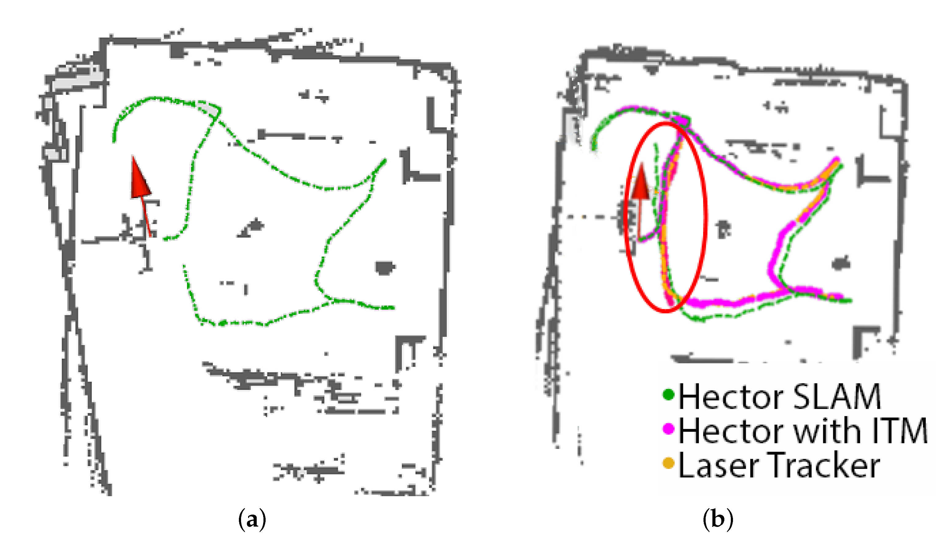
3.2. Map and Pose Correction in 2-D SLAM

Adopting our algorithm into 2-D SLAM requires modification of grid map updating operation. Using Hector SLAM as an example, with $q^{*}$ and $t{r}^{*}$ found in Equation (1), the next step is to identify the current system pose and the grid cells on the map that require correction. Using Hector SLAM as an example, the system pose is recorded as $P=\{p_x,p_y,\psi \}$ where $\psi$ indicates the current system orientation. Converting the quaternion, $q*$, in Equation (1) to a rotation matrix R allows us to directly update the system into a new pose using Equation (2).

$$P=\{(p_x+t{r}_x^{*}),(p_y+t{r}_y^{*}),\psi \oplus {\psi }_R^{*}\}$$

(2)

Grid-map only stores the probability of having obstacles in each grid. In order to find a collection of grids corresponding to a section of trajectory, we have modified the grid map to also store a timestamp. This timestamp records the last time when the scan matcher updated the grid. The sets of grids updated during T are timestamped with t where $t\in T$. Combining the timestamp from both the trajectory points and the grids provides the functionality of selecting grid cells that belong to a certain period of the SLAM process.

In this work, the selection of grid cells with a timestamp is not based on the entire grid map. Instead, to speed up the process, the correction is based on a subset of the grids. A sliding window is made according to the center of the matching trajectory. Let $(Mx,My)$ be the mean value of the section of trajectory. Assume the map resolution is $res$, the LiDAR range is d. The selection window of grid cells $(x,y)$ is :

$$\begin{array}{c}\hfill (\frac{Mx}{res}-\frac{d}{res}p)<x<(\frac{Mx}{res}+\frac{d}{res}p)\\ \hfill (\frac{My}{res}-\frac{d}{res}q)<y<(\frac{My}{res}+\frac{d}{res}q)\end{array}$$

(3)

p and q are a pair of window size parameters which can be changed to better fit the selection window size for a particular LiDAR scanning range.

Equation (4) shows the translation from Equation (1) scaled into the grid map coordinate system.

$$\widehat{tr}=\frac{tr}{res}$$

(4)

With selected grids and the scaled translation, for a collection of grids $G=\left\{g_{t_u},\dots ,g_{t_v}\right\}$ where $\{t_u,\dots ,t_v\}\in T$, a transform of G can be rewritten as:

$$I\left(G\right)=R·G+\widehat{tr}$$

(5)

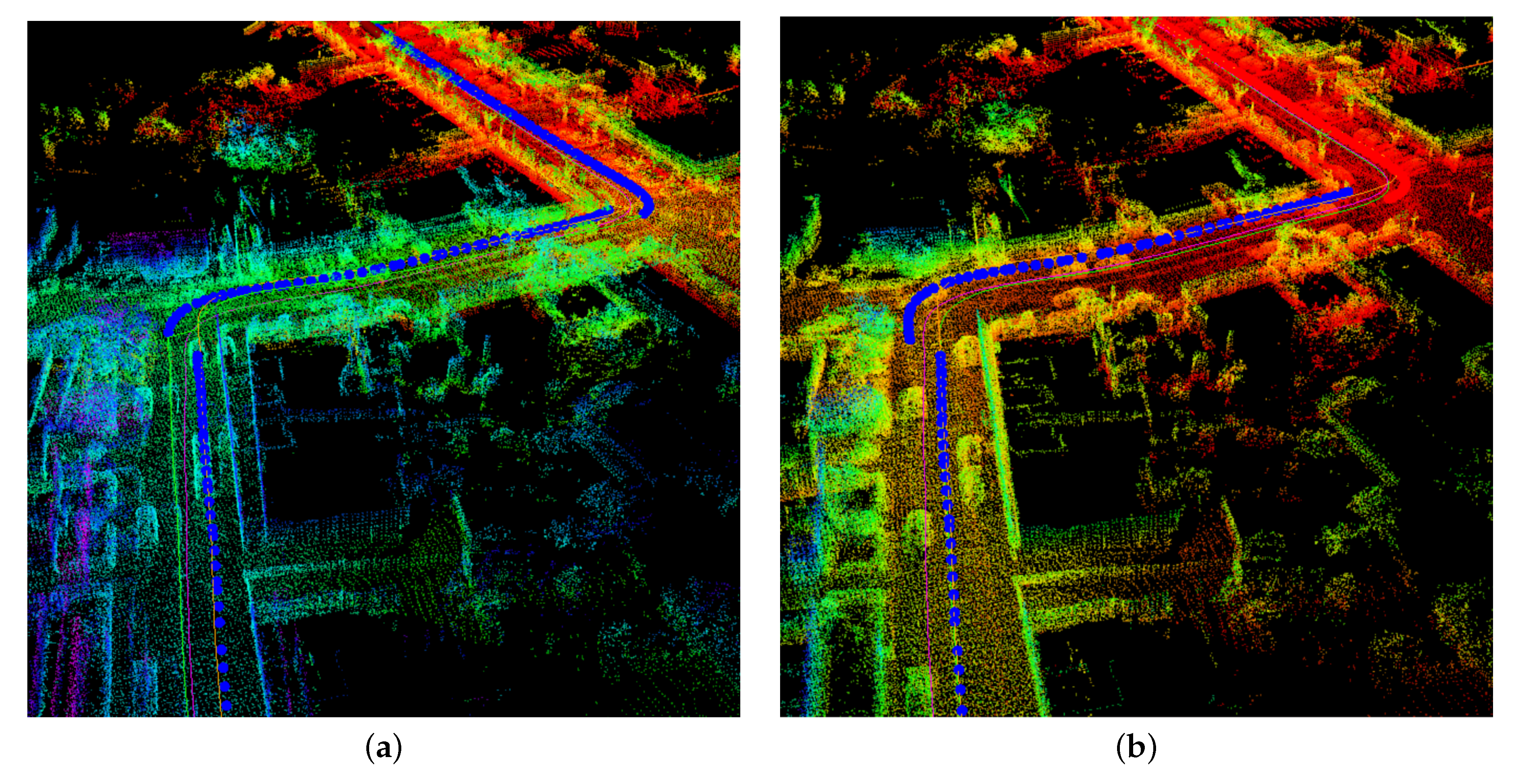
3.3. Pose Interpolation and Correction in 3-D Point Clouds

LOAM is one of the state-of-art LiDAR odometry algorithms at the moment of writing this article. As reviewed in Section 2, LOAM uses the current LiDAR frame to match with the previous frame and submaps respectively. This helps the system to reduce drift errors, especially when traveling on a built map. However, drifting is still obvious if mapping on an uncharted path. As shown in Figure 3, the LiDAR Odometry is the high frequency odometry of LOAM where the current system pose at t is purely dependent on the previous pose at $t-1$. The LiDAR to map trajectory indicates the low frequency odometry where the current system pose is matching with the surrounding submap. The orange line shows the trajectory recorded by the GPS module. Starting at the origin of the coordinate system, the gap developed between the GPS reading and the LOAM odometry.

Unlike 2-D grid maps, 3-D point clouds maps are much denser. The large number of points and high updating frequency on the map make mapping result corrections unrealistic. Therefore, we only focus on pose correction in 3-D implementation. Once a correction is triggered, relocating the LiDAR frame to a new pose will result in a dislocation on the map. Spherical linear interpolation (Slerp) can significantly smooth the process as fractions of the transform are evenly applied to a series of future system pose estimations. Figure 4 shows a comparison of mapping results with and without Slerp.

The mapping result in Figure 4a illustrates a sharp pose correction without Slerp smoothing. The relocation of the LiDAR frame results in a point clouds ghosting. In Figure 4b, the ghosting problem is notably improved by the Slerp process. In this particular experiment, a transform is divided into 20 steps and interpolated into the LiDAR-Submap matching process in LOAM. The process runs in 4 $\mathrm{hz}$, thus takes about 5 s to complete the Slerp.

4. Experiments

A series of experiments were conducted based on the proposed ITM algorithm. The software in this work is constructed using the framework of the Robotic Operating System (ROS) [55]. Three sets of experiments were performed to evaluate the performance of the ITM algorithm with Hector SLAM and LOAM. Figure 5 illustrates the setups used in these experiments. Figure 5a is a pair of handheld units and a laser tracker. In this setup, the handheld unit runs Hector SLAM and the reference trajectory is provided by the Leica LT-500 laser tracker. In Figure 5b, a handheld unit similar to (a) is grouped with a GPS module as the reference trajectory. Both (a) and (b) are used for Hector SLAM testing. Experiments with LOAM were performed using the KITTI dataset. All the tests were performed using an Intel^® Joule^TM 570x with quad-core running at 1.7 GHz and 4 GB of RAM.

4.1. Indoor Experiment with Hector SLAM

The first set of experiments was taken in a room in our lab. As shown in Figure 5, this experiment uses a RpLiDAR A2 and a Leica laser tracker LT-500. In this set-up. LiDAR was fixed on top of a handheld device. The reference trajectory was provided by the laser tracker. The laser tracker was placed in the middle of the room. The room was full of laboratory equipment and two transparent walls. The main challenges for Hector SLAM to perform mapping in this environment were due to three factors: the low resolution of RpLiDAR, the arbitrary obstructions in the space, and the two glass walls that generate noise in the LiDAR. The room is about 11 m long, 7 m wide. During the experiment, the handheld device remained about 1.3 m above the floor and traveled through the room. The device visited some corners of the room and followed by a sharp turn. It traveled close to the transparent wall and eventually returned to the starting position of the experiment.

Figure 6a shows the mapping results from the native Hector SLAM algorithm. The SLAM trajectory indicates the trajectory estimated by Hector SLAM. A noticeable mapping error can be seen on the left side of the map as the unit traveling close to the glass wall. This results in a map deformation and a misaligned wall.

Figure 6b illustrates another mapping attempt with the ITM involved. Comparing with the result in Figure 6a, the ITM algorithm successfully detected the misalignment of the Hector trajectory and the reference trajectory. A match was found between trajectories in the circled area. As the result, the ITM process successfully restored the misaligned wall on the left side of the map. While correcting the pose of the system, it also transforms the grids inside the sliding window. The searching sliding window is set to twice of the LiDAR sensing range in this particular test.

In the experiment, the ITM algorithm only triggered once as the threshold is set relatively high. Figure 7 shows a detailed illustration of the section of trajectories that involved in the correction process circled in Figure 6b. It is indicated in the figure that Hector trajectory is aligned to the laser tracker trajectory.

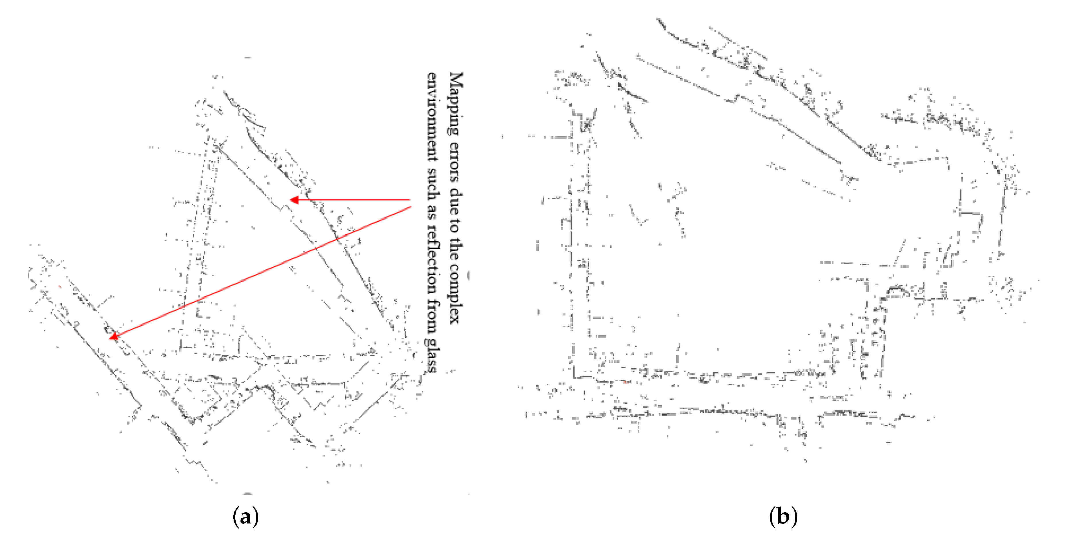
4.2. Indoor-Outdoor Experiment with Hector SLAM

The second set of experiments took place in an indoor-outdoor mixed environment. With the device shown in Figure 5b, this experiment uses a Hokuyo UTX-20L as the LiDAR sensor and a GPS modular to provide reference trajectory. The experiment was conducted around Building 37 of Monash University, with part of the trip through an indoor corridor. Readings from GPS is filtered by an EKF. As the GPS sensor stops providing readings when entering indoor areas, the reference trajectory is only available partially in the experiment. The ITM algorithm iteration cycle is set to 30 s.

In this experiment, the handheld device is held about $1.3$ m above the ground. It started from the South entrance of the building (Figure 8a). After that, it went through a long indoor corridor before exiting the building from an automated glass door. There is a featureless open space outside the North exit of the build. Then the device entered an alley surrounded by metal meshes and plants. ITM algorithm is triggered twice during the experiment, as shown in Figure 8b with the solid trajectory. The dash trajectory is the outcome of original Hector SLAM. The diamond trajectory is formed from the readings from the GPS module. The effects of ITM are evident as illustrated in Figure 8b. With the device started at $(x=-50,y=-20)$ on the chart and traveled clockwise, it finishes the experiment by returning to the starting point. The trip goes around the building a bit more than one lap. Noting that the trajectory from the GPS is not available while traveling through the corridor.

Figure 9 shows a comparison between mapping results of Hector SLAM with and without the proposed algorithm. In Figure 9a, without the ITM algorithm, the Hector SLAM is vulnerable to the complex environment. Two significant mapping errors were recorded during traveling through the corridor and entering the featureless space via the automated glass door. The heavily twisted mapping results accumulated through the mapping process and eventually cause overlapping of map sections. These problems are improved using ITM in Figure 9b with most of the twisted map sections restored. The two successfully triggered the ITM process helps the Hector algorithm to relocate the system pose on the map after major failures.

To quantify the effects of the proposed ITM algorithm, assume position difference, $Pd$, is the difference of positions in the Hector trajectory with and without ITM compares with the position estimation from the GPS with EKF. In Equation (6), x and y are the coordinates of position estimation in the GPS frame. $\widehat{x}$ and $\widehat{y}$ are the coordinates of position estimation from a corresponding algorithm.

$$Pd\left(t\right)=\sum _{i=1}^k\sqrt{{\left(x_i-{\widehat{x}}_i\right)}^2+{\left(y_i-{\widehat{y}}_i\right)}^2}$$

(6)

In Figure 10, the difference between the original Hector trajectory and the GPS reading is shown in the solid line. The dashed line indicates the difference between Hector with ITM and GPS reading. The gap on the chart represents the time period without GPS reception. Two sharp drops can be clearly seen on the dashed line. These drops indicate the correction of system pose caused by the ITM algorithm. Each ITM correction reduces the position difference between Hector position estimation and GPS reading.

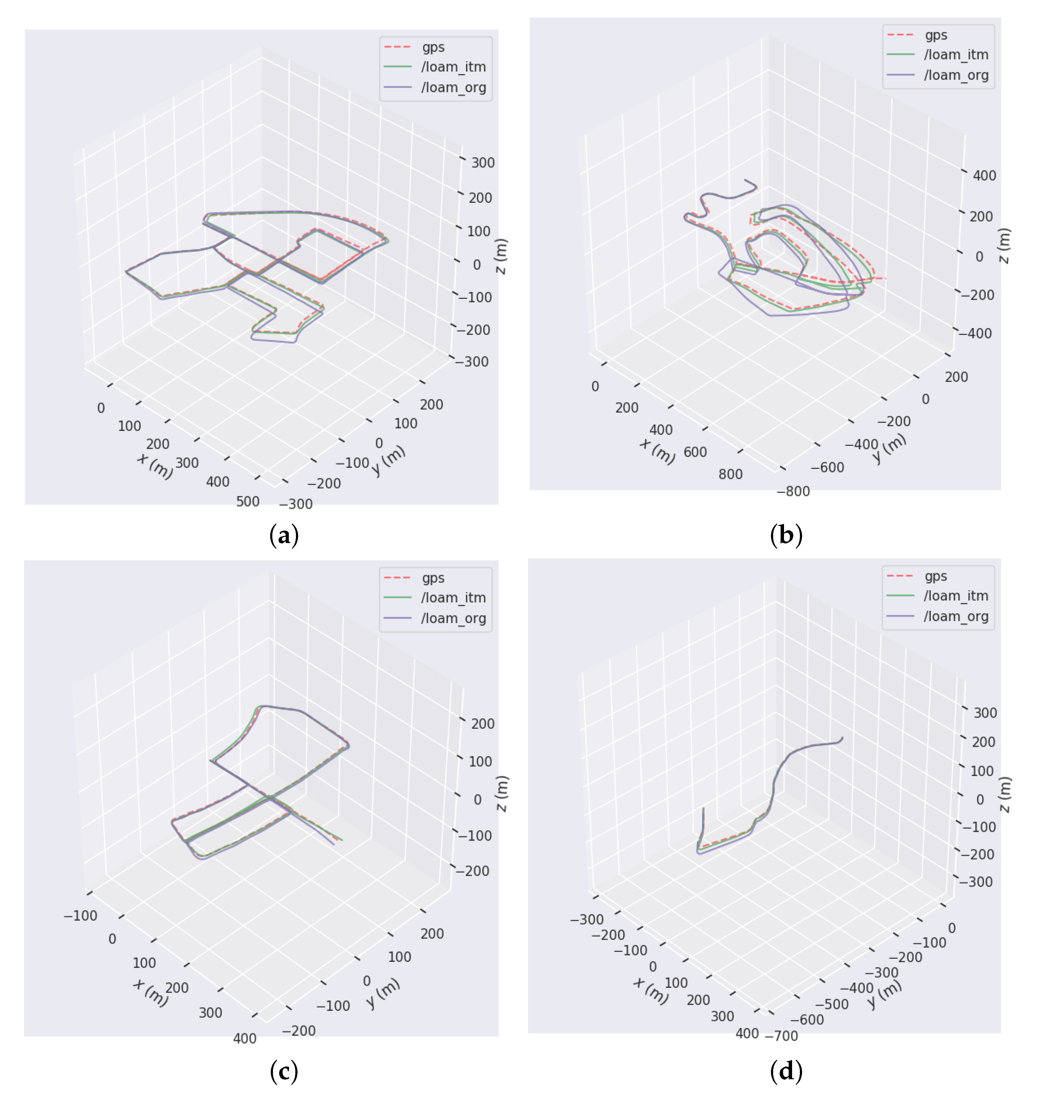
4.3. Testing on KITTI Dataset with LOAM

Under 3-D category, we chose to evaluate our method with LOAM using KITTI dataset. KITTI Visual Odometry and SLAM dataset is a benchmarking dataset featuring LiDAR, stereo camera, GPS and other sensors. The subset of scenes we selected to test our algorithm features streets in the suburban area of Karlsruhe and highways. We used LOAM with LiDAR readings only as the targeting 3-D mapping algorithm. GPS readings were selected as the reference trajectory. Similar to the experiment with Hector SLAM, we have interpolated the LOAM algorithm with an extra level of mapping operation. After each qualified match, a translation is applied to the current system pose. As explained previously in Section 3, 3-D map restoration is computationally expensive. Instead, we used Slerp to smooth the translation and rotation in these tests. The detailed comparisons between original LOAM, LOAM with ITM interpolation, and GPS frame are shown in Figure 11. The proposed ITM algorithm successfully identified the gap between the GPS trajectory and the LOAM trajectory. The results of the pose correction can be seen in Figure 12 with the comparison between each axes.

In our tests, LOAM presents the state-of-art LiDAR SLAM accuracy. Its pose estimation for x and y axes are almost identical to the GPS reading in most tests. However, As illustrated on the charts, its z axis estimation suffers drifting errors. This problem is more obvious in Figure 12b,d where the car is traveling in an open loop. The drifts on the z axis are significantly reduced on the LOAM with ITM trajectories where poses were aligned with the GPS reading. Taking KITTI 02 dataset as an example, the original LOAM results in severe mapping errors in multiple locations on the map. Figure 13 illustrates a comparison of one of the major mapping errors during the tests where LOAM produces overlapped streets. With ITM, the situation was greatly improved as most of the streets were correctly aligned during the mapping.

5. Conclusions and Discussion

Large noise distribution of GNSS and other 3 degree-of-freedom absolute positing sensors makes them difficult to be integrated into high frequency tightly-coupled SLAM algorithms. However, the trajectory observed from these sensors could still be used to improve the robustness and accuracy of a SLAM system. In this paper, we have demonstrated a different approach to improve the robustness and accuracy of a SLAM process. The proposed ITM method finds the rotation and translation between a section of a pair of trajectories and uses the information to recover the system pose. The experiments showed that interpolating the rotation and translation to the current system pose of a SLAM algorithm with the proposed ITM method could help the system to recover its position and orientation. Additionally, with enough computing power, this information could also be applied to the map to restore mapping results. Furthermore, the ITM algorithm does not need to be applied continuously. Instead, it can be invoked at any time when the reference frame is available. This particularly suits the application of large scale indoor-outdoor mixed mapping environments where GNSS information is only partially available. Thus, the most important limitation of the proposed approach is when the GNSS information is not available.

Finally, as the continuation the present work, it is intended to investigate the accuracy of the proposed SLAM algorithm in difficult lighting situations such as at night, tunnels, or the presence of fog/rain which is a challenging problem in the SLAM realm (Supplementary Materials).

References

1. Zhan, Z.; Jian, W.; Li, Y.; Yue, Y. A slam map restoration algorithm based on submaps and an undirected connected graph. IEEE Access 2021, 9, 12657–12674. [Google Scholar] [CrossRef]
2. Meng, Q.; Guo, H.; Zhao, X.; Cao, D.; Chen, H. Loop-closure detection with a multiresolution point cloud histogram mode in lidar odometry and mapping for intelligent vehicles. IEEE/ASME Trans. Mechatron. 2021, 26, 1307–1317. [Google Scholar] [CrossRef]
3. Yang, T.; Li, P.; Zhang, H.; Li, J.; Li, Z. Monocular Vision SLAM-Based UAV Autonomous Landing in Emergencies and Unknown Environments. Electronics 2018, 7, 73. [Google Scholar] [CrossRef] [Green Version]
4. Sadeghi Esfahlani, S.; Sanaei, A.; Ghorabian, M.; Shirvani, H. The Deep Convolutional Neural Network Role in the Autonomous Navigation of Mobile Robots (SROBO). Remote Sens. 2022, 14, 3324. [Google Scholar] [CrossRef]
5. Kim, P.; Chen, J.; Cho, Y.K. SLAM-driven robotic mapping and registration of 3D point clouds. Autom. Constr. 2018, 89, 38–48. [Google Scholar] [CrossRef]
6. Kohlbrecher, S.; Von Stryk, O.; Meyer, J.; Klingauf, U. A flexible and scalable slam system with full 3d motion estimation. In Proceedings of the 2011 IEEE International Symposium on Safety, Security, and Rescue Robotics, Kyoto, Japan, 1–5 November 2011; pp. 155–160. [Google Scholar]
7. Grisetti, G.; Stachniss, C.; Burgard, W. Improved techniques for grid mapping with rao-blackwellized particle filters. IEEE Trans. Robot. 2007, 23, 34–46. [Google Scholar] [CrossRef] [Green Version]
8. Hess, W.; Kohler, D.; Rapp, H.; Andor, D. Real-time loop closure in 2D LIDAR SLAM. In Proceedings of the 2016 IEEE International Conference on Robotics and Automation (ICRA), Stockholm, Sweden, 16–21 May 2016; pp. 1271–1278. [Google Scholar]
9. Vincent, R.; Limketkai, B.; Eriksen, M. Comparison of indoor robot localization techniques in the absence of GPS. In Proceedings of the Detection and Sensing of Mines, Explosive Objects, and Obscured Targets XV. International Society for Optics and Photonics; 2010; Volume 7664, p. 76641Z. Available online: https://spie.org/Publications/Proceedings/Volume/11750 (accessed on 9 July 2022).
10. Segal, A.; Haehnel, D.; Thrun, S. Generalized-icp. In Proceedings of the Robotics: Science and Systems, Seattle, WA, USA, 28 June–1 July 2009; Volume 2, p. 435. [Google Scholar]
11. Censi, A. An ICP variant using a point-to-line metric. In Proceedings of the 2008 IEEE International Conference on Robotics and Automation, Pasadena, CA, USA, 19–23 May 2008; pp. 19–25. [Google Scholar]
12. Besl, P.J.; McKay, N.D. Method for registration of 3-D shapes. In Proceedings of the Sensor Fusion IV: Control Paradigms and Data Structures; International Society for Optics and Photonics: Bellingham, WA, USA, 1992; Volume 1611, pp. 586–606. [Google Scholar]
13. Das, A.; Servos, J.; Waslander, S.L. 3D scan registration using the normal distributions transform with ground segmentation and point cloud clustering. In Proceedings of the 2013 IEEE International Conference on Robotics and Automation, Karlsruhe, Germany, 6–10 May 2013; pp. 2207–2212. [Google Scholar]
14. Das, A.; Waslander, S.L. Scan registration using segmented region growing NDT. Int. J. Robot. Res. 2014, 33, 1645–1663. [Google Scholar] [CrossRef]
15. Merten, H. The three-dimensional normal-distributions transform. Threshold 2008, 10, 3. [Google Scholar]
16. Fossel, J.; Hennes, D.; Claes, D.; Alers, S.; Tuyls, K. OctoSLAM: A 3D mapping approach to situational awareness of unmanned aerial vehicles. In Proceedings of the 2013 International Conference on Unmanned Aircraft Systems (ICUAS), Atlanta, GA, USA, 28–31 May 2013; pp. 179–188. [Google Scholar]
17. Kwak, N.; Stasse, O.; Foissotte, T.; Yokoi, K. 3D grid and particle based SLAM for a humanoid robot. In Proceedings of the 2009 9th IEEE-RAS International Conference on Humanoid Robots, Paris, France, 7–10 December 2009; pp. 62–67. [Google Scholar]
18. Nüchter, A.; Bleier, M.; Schauer, J.; Janotta, P. Continuous-Time SLAM—Improving Google’s Cartographer 3D Mapping. In Latest Developments in Reality-Based 3D Surveying and Modelling; MDPI: Basel, Switzerland, 2018; pp. 53–73. [Google Scholar]
19. Bosse, M.; Zlot, R. Continuous 3D scan-matching with a spinning 2D laser. In Proceedings of the 2009 IEEE International Conference on Robotics and Automation, Kobe, Japan, 12–17 May 2009; pp. 4312–4319. [Google Scholar]
20. Zlot, R.; Bosse, M. Efficient large-scale 3D mobile mapping and surface reconstruction of an underground mine. In Proceedings of the Field and Service Robotics; Springer: Berlin/Heidelberg, Germany, 2014; pp. 479–493. [Google Scholar]
21. Bosse, M.; Zlot, R.; Flick, P. Zebedee: Design of a spring-mounted 3-d range sensor with application to mobile mapping. IEEE Trans. Robot. 2012, 28, 1104–1119. [Google Scholar] [CrossRef]
22. Zhang, J.; Singh, S. LOAM: Lidar Odometry and Mapping in Real-time. In Proceedings of the Robotics: Science and Systems; 2014; Volume 2. Available online: http://www.roboticsproceedings.org/ (accessed on 9 July 2022).
23. Shan, T.; Englot, B. LeGO-LOAM: Lightweight and Ground-Optimized Lidar Odometry and Mapping on Variable Terrain. In Proceedings of the 2018 IEEE/RSJ International Conference on Intelligent Robots and Systems (IROS), Madrid, Spain, 1–5 October 2018; pp. 4758–4765. [Google Scholar]
24. Zhang, J.; Singh, S. Laser–visual–inertial odometry and mapping with high robustness and low drift. J. Field Robot. 2018, 35, 1242–1264. [Google Scholar] [CrossRef]
25. Mur-Artal, R.; Tardós, J.D. Orb-slam2: An open-source slam system for monocular, stereo, and rgb-d cameras. IEEE Trans. Robot. 2017, 33, 1255–1262. [Google Scholar] [CrossRef] [Green Version]
26. Mur-Artal, R.; Tardós, J.D. Visual-inertial monocular SLAM with map reuse. IEEE Robot. Autom. Lett. 2017, 2, 796–803. [Google Scholar] [CrossRef] [Green Version]
27. Campos, C.; Elvira, R.; Rodríguez, J.J.G.; Montiel, J.M.; Tardós, J.D. ORB-SLAM3: An accurate open-source library for visual, visual-inertial and multi-map SLAM. arXiv 2020, arXiv:2007.11898. [Google Scholar] [CrossRef]
28. Lee, Y.C.; Chae, H.; Yu, W. Artificial landmark map building method based on grid SLAM in large scale indoor environment. In Proceedings of the 2010 IEEE International Conference on Systems, Man and Cybernetics, Istanbul, Turkey, 10–13 October 2010; pp. 4251–4256. [Google Scholar]
29. Zhao, L.; Huang, S.; Dissanayake, G. Linear SLAM: A linear solution to the feature-based and pose graph SLAM based on submap joining. In Proceedings of the 2013 IEEE/RSJ International Conference on Intelligent Robots and Systems, Tokyo, Japan, 3–7 November 2013; pp. 24–30. [Google Scholar]
30. Ni, K.; Dellaert, F. Multi-level submap based slam using nested dissection. In Proceedings of the 2010 IEEE/RSJ International Conference on Intelligent Robots and Systems, Taipei, Taiwan, 18–22 October 2010; pp. 2558–2565. [Google Scholar]
31. Chen, L.H.; Peng, C.C. A Robust 2D-SLAM Technology with Environmental Variation Adaptability. IEEE Sens. J. 2019, 19, 11475–11491. [Google Scholar] [CrossRef]
32. Brand, C.; Schuster, M.J.; Hirschmuller, H.; Suppa, M. Submap matching for stereo-vision based indoor/outdoor SLAM. In Proceedings of the 2015 IEEE/RSJ International Conference on Intelligent Robots and Systems (IROS), Hamburg, Germany, 28 September–2 October 2015; pp. 5670–5677. [Google Scholar] [CrossRef] [Green Version]
33. Jiménez, P.A.; Shirinzadeh, B. Laser interferometry measurements based calibration and error propagation identification for pose estimation in mobile robots. Robotica 2014, 32, 165–174. [Google Scholar] [CrossRef]
34. Palomer, A.; Ridao, P.; Ribas, D. Inspection of an underwater structure using point-cloud SLAM with an AUV and a laser scanner. J. Field Robot. 2019, 36, 1333–1344. [Google Scholar] [CrossRef]
35. Shirinzadeh, B. Laser-interferometry-based tracking for dynamic measurements. Ind. Robot. Int. J. 1998, 25, 35–41. [Google Scholar] [CrossRef]
36. Gao, W.; Wang, K.; Ding, W.; Gao, F.; Qin, T.; Shen, S. Autonomous aerial robot using dual-fisheye cameras. J. Field Robot. 2020, 37, 497–514. [Google Scholar] [CrossRef]
37. Kubelka, V.; Reinstein, M.; Svoboda, T. Tracked Robot Odometry for Obstacle Traversal in Sensory Deprived Environment. IEEE/ASME Trans. Mechatron. 2019, 24, 2745–2755. [Google Scholar] [CrossRef]
38. Azim, A.; Aycard, O. Detection, classification and tracking of moving objects in a 3D environment. In Proceedings of the 2012 IEEE Intelligent Vehicles Symposium, Madrid, Spain, 3–7 June 2012; pp. 802–807. [Google Scholar]
39. Asmar, D.C.; Zelek, J.S.; Abdallah, S.M. SmartSLAM: Localization and mapping across multi-environments. In Proceedings of the 2004 IEEE International Conference on Systems, Man and Cybernetics (IEEE Cat. No. 04CH37583), The Hague, The Netherlands, 10–13 October 2004; Volume 6, pp. 5240–5245. [Google Scholar]
40. Collier, J.; Ramirez-Serrano, A. Environment classification for indoor/outdoor robotic mapping. In Proceedings of the 2009 Canadian Conference on Computer and Robot Vision, CRV 2009, Kelowna, BC, Canada, 25–27 May 2009; pp. 276–283. [Google Scholar] [CrossRef]
41. Dill, E.; De Haag, M.U.; Duan, P.; Serrano, D.; Vilardaga, S. Seamless indoor-outdoor navigation for unmanned multi-sensor aerial platforms. In Proceedings of the Record—IEEE PLANS, Position Location and Navigation Symposium, Monterey, CA, USA, 5–8 May 2014; pp. 1174–1182. [Google Scholar] [CrossRef]
42. Lee, Y.J.; Song, J.B. Three-dimensional iterative closest point-based outdoor SLAM using terrain classification. Intell. Serv. Robot. 2011, 4, 147–158. [Google Scholar] [CrossRef]
43. Ilci, V.; Toth, C. High definition 3D map creation using GNSS/IMU/LiDAR sensor integration to support autonomous vehicle navigation. Sensors 2020, 20, 899. [Google Scholar] [CrossRef] [PubMed] [Green Version]
44. Chiang, K.W.; Tsai, G.J.; Li, Y.H.; Li, Y.; El-Sheimy, N. Navigation Engine Design for Automated Driving Using INS/GNSS/3D LiDAR-SLAM and Integrity Assessment. Remote. Sens. 2020, 12, 1564. [Google Scholar] [CrossRef]
45. Gálvez-López, D.; Tardos, J.D. Bags of binary words for fast place recognition in image sequences. IEEE Trans. Robot. 2012, 28, 1188–1197. [Google Scholar] [CrossRef]
46. Caballero, F.; Pérez, J.; Merino, L. Long-term ground robot localization architecture for mixed indoor-outdoor scenarios. In Proceedings of the ISR/Robotik 2014: 41st International Symposium on Robotics, Munich, Germany, 2–3 June 2014; pp. 21–28. [Google Scholar]
47. Mur-Artal, R.; Montiel, J.M.M.; Tardos, J.D. ORB-SLAM: A versatile and accurate monocular SLAM system. IEEE Trans. Robot. 2015, 31, 1147–1163. [Google Scholar] [CrossRef] [Green Version]
48. Qin, T.; Li, P.; Shen, S. Vins-mono: A robust and versatile monocular visual-inertial state estimator. IEEE Trans. Robot. 2018, 34, 1004–1020. [Google Scholar] [CrossRef] [Green Version]
49. Rosinol, A.; Abate, M.; Chang, Y.; Carlone, L. Kimera: An open-source library for real-time metric-semantic localization and mapping. In Proceedings of the 2020 IEEE International Conference on Robotics and Automation (ICRA), Paris, France, 31 May–31 August 2020; pp. 1689–1696. [Google Scholar] [CrossRef]
50. Caruso, D.; Eudes, A.; Sanfourche, M.; Vissière, D.; Le Besnerais, G. An inverse square root filter for robust indoor/outdoor magneto-visual-inertial odometry. In Proceedings of the 2017 International Conference on Indoor Positioning and Indoor Navigation, IPIN 2017, Sapporo, Japan, 8–21 September 2017; pp. 1–8. [Google Scholar] [CrossRef]
51. Liu, Q.; Liang, P.; Xia, J.; Wang, T.; Song, M.; Xu, X.; Zhang, J.; Fan, Y.; Liu, L. A highly accurate positioning solution for C-V2X systems. Sensors 2021, 21, 1175. [Google Scholar] [CrossRef]
52. Wei, W.; Shirinzadeh, B.; Esakkiappan, S.; Ghafarian, M.; Al-Jodah, A. Orientation Correction for Hector SLAM at Starting Stage. In Proceedings of the 2019 7th International Conference on Robot Intelligence Technology and Applications (RiTA), Daejeon, Korea, 1–3 November 2019; pp. 125–129. [Google Scholar]
53. Wei, W.; Shirinzadeh, B.; Nowell, R.; Ghafarian, M.; Ammar, M.M.; Shen, T. Enhancing solid state lidar mapping with a 2d spinning lidar in urban scenario slam on ground vehicles. Sensors 2021, 21, 1773. [Google Scholar] [CrossRef]
54. Geiger, A.; Lenz, P.; Urtasun, R. Are we ready for Autonomous Driving? The KITTI Vision Benchmark Suite. In Proceedings of the Conference on Computer Vision and Pattern Recognition (CVPR), Providence, RI, USA, 16–21 June 2012. [Google Scholar]
55. Stanford Artificial Intelligence Laboratory. Robotic Operating System; Stanford Artificial Intelligence Laboratory: Stanford, CA, USA, 2018. [Google Scholar]
Figure 1. Explanation of the Proposed ITM Process.
Processes 10 01433 g001
Figure 2. An Example of Trajectory Alignment in ITM.
Processes 10 01433 g002
Figure 3. Trajectory from LOAM (Dataset 01 from KITTI VO/SLAM [54]).
Processes 10 01433 g003
Figure 4. (a) 3-D Points cloud without Slerp, (b) and 3-D Points cloud with Slerp.
Processes 10 01433 g004
Figure 5. Two different setups used in the experiments. (a) The handheld device with Laser Tracker. (b) The handheld unit with GPS.
Processes 10 01433 g005
Figure 6. Mapping and trajectory in RMRL lab. (a) Native Hector SLAM Process; (b) A ITM interpolated Hector SLAM Process.
Processes 10 01433 g006
Figure 7. Zoom-in on the section of trajectories in the active ITM process.
Processes 10 01433 g007
Figure 8. Experiment around Building 37 with Trajectories. (a) Satellite photo of Building 37 with trail highlighted. (b) Trajectories compared in the Building 37 experiment.
Processes 10 01433 g008
Figure 9. Comparison of Mapping Results with and without ITM near Building 37 on Monash Campus. (a) Mapping Result with original HectorSLAM. (b) Mapping Result with Proposed ITM Algorithm.
Processes 10 01433 g009
Figure 10. Position difference comparison of Hector SLAM with and without ITM.
Processes 10 01433 g010
Figure 11. Comparison of Mapping Results with and without ITM Using KITTI Dataset. (a) KITTI Dataset 00. (b) KITTI Dataset 02. (c) KITTI Dataset 05. (d) KITTI Dataset 10.
Processes 10 01433 g011
Figure 12. Comparison of Mapping Results with and without ITM Using KITTI Dataset. (a) KITTI Dataset 00. (b) KITTI Dataset 02. (c) KITTI Dataset 05. (d) KITTI Dataset 10.
Processes 10 01433 g012
Figure 13. Mapping Results of LOAM with and without ITM on KITTI Dataset 02. (a) LOAM without ITM. (b) LOAM With ITM.
Processes 10 01433 g013
Publisher’s Note: MDPI stays neutral with regard to jurisdictional claims in published maps and institutional affiliations.