Article

AgroAId: A Mobile App System for Visual Classification of Plant Species and Diseases Using Deep Learning and TensorFlow Lite

Department of Computer Science and Engineering, American University of Sharjah, Sharjah P.O. Box 26666, United Arab Emirates
*
Author to whom correspondence should be addressed.
Informatics 2022, 9(3), 55; https://doi.org/10.3390/informatics9030055
Submission received: 23 May 2022 / Revised: 3 July 2022 / Accepted: 8 July 2022 / Published: 26 July 2022
(This article belongs to the Special Issue Applications of Machine Learning and Deep Learning in Agriculture)

Abstract

:
This paper aims to assist novice gardeners in identifying plant diseases to circumvent misdiagnosing their plants and to increase general horticultural knowledge for better plant growth. In this paper, we develop a mobile plant care support system (“AgroAId”), which incorporates computer vision technology to classify a plant’s [species–disease] combination from an input plant leaf image, recognizing 39 [species-and-disease] classes. Our method comprises a comparative analysis to maximize our multi-label classification model’s performance and determine the effects of varying the convolutional neural network (CNN) architectures, transfer learning approach, and hyperparameter optimizations. We tested four lightweight, mobile-optimized CNNs—MobileNet, MobileNetV2, NasNetMobile, and EfficientNetB0—and tested four transfer learning scenarios (percentage of frozen-vs.-retrained base layers): (1) freezing all convolutional layers; (2) freezing 80% of layers; (3) freezing 50% only; and (4) retraining all layers. A total of 32 model variations are built and assessed using standard metrics (accuracy, F1-score, confusion matrices). The most lightweight, high-accuracy model is concluded to be an EfficientNetB0 model using a fully retrained base network with optimized hyperparameters, achieving 99% accuracy and demonstrating the efficacy of the proposed approach; it is integrated into our plant care support system in a TensorFlow Lite format alongside the front-end mobile application and centralized cloud database. Finally, our system also uses the collective user classification data to generate spatiotemporal analytics about regional and seasonal disease trends, making these analytics accessible to all system users to increase awareness of global agricultural trends.

1. Introduction

Agriculture and plant cultivation often requires significant specialized knowledge about species, diseases, and the complex characteristics of their combinations, since the same single disease can have varying symptoms and treatments depending on the particular species affected [1]. As such, it can easily become a tedious and unsuccessful task to try to recognize the potential disease affecting a specific plant using the naked eye and to then know the correct treatments and preventions to combat the disease for the particular species at hand. This struggle is especially common for novice agriculturalists, who often have yet to develop the specialized experiential “expert” knowledge required to successfully execute this type of early, direct human-eye assessment, which can in turn lead to frequent crop loss as a result of their inaccurate plant disease diagnosis [1,2]. Thus, AI researchers have been working on providing suitable solutions and products that use computer vision technology to serve as a practical supplement to the traditional human-eye detection, instead relying on deep learning networks that have previously presented promising results for the accurate recognition and classification of complex image-based features. This approach offers an opportunity to create a system that could automatically detect and label a plant’s species-and-disease combination from a simple image of the plant, thereby helping gardeners accurately assess a plant’s health and providing the appropriate guidance to effectively care for the plant and sustain successful plant growth. A mobile solution using this AI approach then gives new gardeners easy access to have automated, early-stage, expert-level diagnosis at hand without them needing to personally know all the required plant care information themselves [2].
Deep learning is a popular artificial learning approach that is often used for developing complex predictive algorithms; using programmable layered structures known as neural networks, deep learning models will process complex data to extract relevant features and learn from them, applying the learnt concepts to then make informed decisions. The models continually attempt to evolve and improve their accuracy automatically to make more intelligent decisions for tasks that include pattern recognition and automated classification [3]. This advanced element of continually adapting allows deep learning models to act more like independent learners. However, to develop models that are able to successfully adapt independently takes a computationally-complex process that often requires more extensive training, stronger infrastructure, and large amounts of data [3]. To alleviate some of this computational complexity, the approach of transfer learning is often adopted, where a neural network that has been previously trained for a similar task is used as the base network for a new, related task that builds on the previously gained knowledge to develop a solution for the new problem. Combining a well-trained, intelligent classification model with the accessibility and indispensability of mobile devices creates the perfect setting for a portable [species–disease] classification and plant care support system for small-scale gardeners.
In this paper, we discuss the development of our proposed mobile app system (“AgroAId”). Our proposed solution first focuses on developing an automated multi-label classification model to identify the [species-and-disease] combinations of various plants non-invasively by using images of the plant leaves as its input data. We will focus on using mobile-optimized deep learning models and incorporating a transfer learning approach to develop the best model for our domain. The proposed mobile app system will then incorporate an additional developed backend storage, as well as providing subsequent plant care guidance to users post-classification.
Our main contributions for the proposed solution can be split into two main phases: the models’ development and selection phase; and the system design and deployment phase. The first phase will focus on developing and training several lite, mobile-optimized deep learning models to investigate the effects on model performance when: varying the retrained portions of the base networks (the transfer learning approach); using different convolutional neural network (CNN) architectures; and varying the network hyperparameters. A brief comparative analysis between the developed CNN models will evaluate them based on several parameters including the accuracy, F1-score, confusion matrices and more, to determine the best model for our classification task. The best-performing model will then be integrated into the system designed and deployed in the second phase of the project. The developed proposed system will consist of: a front-end mobile application, which acts as the primary system touchpoint for users; a centralized back-end database, which stores both user-specific and user-wide system data; and the integrated classification model, converted into a TensorFlow Lite file format. Through the application system, the gardeners will be able to complete the project goals of inputting an image of their plant leaf and classifying the [species–disease] combination, as well as accessing additional plant care support features. The system will also use the collective users’ classification results to generate new spatiotemporal analytics about the global agricultural trends for the identifiable species-and-disease combinations, providing these analytics to system users to allow them to further expand their knowledge about species, diseases, and horticulture as a whole.
The paper is organized as follows. Section 1.1 covers related works in the field. Section 2 details the proposed methodology. Section 3 presents the experimental results of the models’ development, with the respective results discussion in Section 4. Section 5 details the proposed system’s implementation and integration. Finally, Section 6 concludes the paper with a summary of the key details and potential future work.

1.1. Literature Review

Below, we include some sources related to our proposed research project, covering the current state of the field and discussing some existing solutions and findings. The field work covers the use of deep learning algorithms to extract plant information using image processing techniques, pre-trained CNNs, and mobile-based solutions. The main works we will reference throughout this article are mentioned separately. Upon outlining the reviewed works, we will compare them to our project to differentiate between our proposed solution and the existing solutions available, thereby identifying the originality of our project.

1.1.1. Image Processing and Automated Disease Classification Solutions

The authors in [4] chose to focus on improving image segmentation for particularly “noisy” plant disease images, using a quantum particle swarm optimization (QPSO) algorithm for segmenting the images and an ontology-based classification process after the feature extraction was completed. With a desire to address food security issues, the authors in [4] classified 12 plant leaf species to cover 22 diseases, reaching an accuracy of 86.22% using their proposed method. The findings in [4] concluded that their proposed segmentation approach, while initially more complex than traditional methods, prove to be more time- and effort-efficient overall for removing noise from plant images “up to noise level σ = 70”, and their suggested “enhanced plant disease ontology” classification approach showed improvement over other state-of-the-art ontology algorithms.
Similarly focusing on plant image processing, the authors in [5] aim to tackle nitrogen deficiency—one of the most common nutritional problems that affects plants—by creating an automated, image-based, early detection system as an efficient, non-destructive method of monitoring plant health and growth. A computer vision-guided system is used to examine cucumber crops and detect nitrogen deficiency by observing color changes in the plants’ stems and leaves by autonomously extracting textural plant features, including entropy, energy, and homogeneity, to determine overall plant growth and health status, as well as using these features as markers for timely detection of nitrogen deficiency. The system architecture included a robotic camera moving module, an image acquisition/processing module, and a data analysis/storage module; the images were transferred from the cameras on the robot to a remote computer using a wireless module. The findings in [5] concluded that the system was able to successfully identify nitrogen-deficient cucumbers two days before visual stress symptoms were detected by human vision, confirming the health benefits that can come from using an AI-based detection system.
In [6], the authors focus on the automated image classification of broadleaf and grass weeds to address common weed infestations in the Alfalfa plant. The method consisted of using 4 different input image sizes, four neural network architectures (AlexNet, GoogLeNet, VGGNet, and ResNet), and four different network optimizers to compare between the variations and investigate the effects of the respective changes on weed detection. The findings in [6] concluded that an increased input image size resulted in a reduced classification accuracy across all the networks developed, and that the most effective classifier when trained with the concluded best input size and optimizer was VGGNet, while ResNet was the least effective classifier.
Some recent works have focused on using image augmentation and complex feature extraction to address the identification of rice leaf diseases in particular [7,8]. In [7], seven image augmentation techniques were used to expand an initial rice leaf image dataset from 2215 images to 12,684 images, employing Gaussian blur augmentation, Laplacian sharpening, contrast enhancement, shifting, rotation, and flipping. A Resnet model was developed to address the complex feature extraction required and was trained with 10 epochs, a learning rate of 0.001, and an Adam optimizer to achieve a high accuracy and minimal validation loss. Meanwhile, the authors in [8] opted to create a new architecture named MobInc-Net, consisting of a modified Inception module created using depth-wise convolutions and combined with a pre-trained MobileNet module to create the foundation of the feature extractor and classifier. The new model in [8] was trained on a local dataset that classifies 12 categories of rice diseases in 1000 images with complex field backgrounds, and resulted in an average accuracy of over 97% when tested on both a local and public dataset.

1.1.2. CNNs and Transfer Learning

Transfer learning is one of the most popular approaches currently used for developing deep learning and artificial intelligence models. Transfer learning involves fine-tuning pre-trained neural networks to create new models efficiently with less complex training processes.
In [9], deep learning techniques are used to assist in the early detection of a single newly-developed disease: the Gray Leaf Spot disease in tomato plants. The authors in [9] use the MobileNetv2-YOLOv3 neural network model, which occupies very little memory (28 MB), and produced overall results with an accuracy of 92.53%.
In [10], image segmentation and multi-label classification are used to classify four different cucumber leaf diseases (anthracnose, downy mildew, powdery mildew, target leaf spot) using a deep CNN base network. The dataset used in [10] contains images of cucumber diseases in field conditions, and the CNN developed achieved an accuracy of 93.4%.
A similar comparative multi-class work was conducted in [11], which focused on investigating the use of transfer learning to create neural networks specifically for multi-class plant image classification. The public PlantVillage dataset was used in [11], which contains images for 38 disease classes and 1 background class, and 5 different CNN architectures were studied: VGG16, InceptionV3, InceptionResNet, ResNet50, and DenseNet169. The final chosen model in [11] was a ResNet50 model, which achieved a precision score of 94%, recall and F1-scores of 94%, and an accuracy percentage of 98.2%.
In [12], the authors used AlexNet, GoogLeNet, and ResNet50 CNN models to extract deep features and use them to train a Support Vector Machine (SVM) classifier in order to classify tomato plant diseases and pests from the input leaf images. A hold-out validation method was used to train and test the module on a dataset of 18,835 images belonging to 9 diseased classes and 1 healthy class, with an overall accuracy rate of 96%.
In [13], the authors use deep bilinear CNNs for the multi-class classification of plant diseases, using a subset of the PlantVillage dataset to classify 54,305 images in 38 classes. Focusing on designing a solution to leverage scalability, the authors in [13] use a fine-tuned VGG model and pruned ResNet model for their feature extraction, connecting them to fully-connected dense networks. Although a large-sized CNN system is employed, the method of [13] states that the hyperparameters were tuned to attempt to reach a faster convergence while maintaining the generalization properties of the CNNs. The findings of the work reported an accuracy of 94.9% and found a low deviation in the accuracy (0.27%) when scaling the test samples by five times [13].
In [14], the authors focused on using transfer learning techniques alongside deep CNNs to classify various plant species into “healthy” and “infected” subclasses, comparing a mix of architectures including VGG16, VGG19, ResNet, DenseNet, XCeption, and MobileNet pre-trained models. The results found that feature extraction was most successful in the VGG models, reaching average accuracies of 97% between the two models, and also concluded that the VGG models experienced the least variation of performance with the data imbalance and intensifying network depths that were required for the complex feature extraction the authors aimed for. The authors in [14] reported that the learning works became over-sophisticated for the other models as the depth of the layers intensified in the networks, highlighting that the ResNet and DenseNet models in particular kept almost exactly the same features extracted from their earlier input layers because of the frequent skip connections in their architectures.

1.1.3. Plant-Based Mobile Application Solutions

In [15], the authors outline the technical processes for pre-processing a plant image in order to extract its important visual features as a separate step prior to feeding the extracted features into a neural network classifier, with the aim of improving its performance when classifying a plant disease. The machine learning algorithms covered are explained with particular focus on their applications to mobile classification, including covering K-means clustering for image segmentation and mobile model conversion. The example mobile application in [15] allows users to take an image of a plant to be classified using the device’s camera, similar to our intended application input (but does not include an option to upload a photo from the device’s gallery, which is included in our system).
In [16], a mobile application solution for plant disease classification called “iDahon” was presented by the University of Philippines with the aim of enhancing terrestrial disease identification due to the economy of the Philippines being significantly dependent on agricultural export. The authors in [16] used a total of 1650 images to train the model, using a training:validation:testing split of 60:20:20, and concentrated on 11 classes of leaf diseases pertaining to terrestrial diseases common in the Philippines. The training datasets are loaded in and processed using the TensorFlow library, with Python as the scripting language chosen to develop the models, then Docker cloud is used to load the mobile-integrated model for virtual training and testing. The system in [16] also accommodated two input sources for users: either taking a picture of the specified plant using the camera, or uploading a pre-existing image from the mobile gallery.
In [17], the authors used new, mobile-captured images taken in field conditions to create their own dataset of healthy and diseased plum images, using additional data augmentation to generate 19 different versions of each image to result in a total dataset of 100,000 images. The authors classified five plum classes—healthy; brown rot; nutrient deficiency; shot hole; and shot hole on leaf—using four developed models: AlexNet; VGG16; Inception-v1; and Inception-v3. The findings in [17] concluded that the Inception models performed the best, where the overall performance of the best model was found to be 88.42% when tested with a 100 image test set.
In [18], we reported an initial implementation of our application. In this paper, on the other hand, we expand on the proposed models, implementation, integration into the mobile app, and the experimental results.
Below, we present the main sources that we used as the basis of our model implementations phase; these sources were used in order to better understand transfer learning and mobile-optimized CNNs, and to improve on the work presented in a pre-existing solution, in line with the aims of our comparative model analysis.
The main dataset we have chosen to use to train our deep learning models on is the PlantVillage dataset, which consists of over 61,486 images belonging to 39 classes, where each class represents a different species-and-disease combination, along with 1 additional ‘background class’. In [19], the authors present an Android mobile application system that classifies plant diseases using integrated lite deep neural networks. The research covered the implementation of three neural networks: MobileNet, MNasNet, and InceptionV3, and used the same dataset we have chosen to work on (the PlantVillage dataset). The training of the models developed was conducted over 30 epochs and with a learning rate of 0.01 and had a training:validation:testing split of 60:20:20. The work in [19] was particularly interesting as it included a comparative analysis between the 3 models developed, considering aspects such as the memory use and latency levels alongside the standard records of accuracy, precision, recall and F1-scores results. On average, the models were able to achieve scores of approximately 90%. In [20], a four-scenario transfer learning approach is outlined for training comprehensive neural networks; we applied this four-scenario approach throughout our model development and assessment processes as a comparative guideline for our transfer learning investigation.

1.2. Aim of Work and Principal Conclusions of Originality

Our research project aims to build a mobile system that identifies the [species–disease] combination of a plant based on an input image of the plant’s leaf using an integrated CNN classification model. The research project will center around a purely- software-based system design consisting of a mobile application, a centralized database, and an integrated deep learning model—this will be the best-performing model as determined by our brief comparative analysis between the various classification models developed.
While there are existing solutions that have previously investigated using deep learning networks to classify plant images or implemented simple mobile application prototypes [15,16], our approach here offers a slightly different perspective. The approach we have adopted for this particular project—our investigative aims, chosen networks and assessment criteria for our models; our focus on creating a mobile-optimized model, and supporting over 35 disease classes in our robust multi-label classification model; combined with our additional, more comprehensive system features available beyond the image classification—present a fairly new approach for our work.
To elaborate, the user analytics options that we aim to present to the user, and the extra functionalities for supported plant care guidance, are not all available in other existing applications. Beyond the classification, the system application will outline the specific symptoms and steps for treatment of the disease for the particular species at hand, serving to educate the novice gardener users on the expert agricultural knowledge. This aspect is new and differs from the other app ideas and completes the purpose of our platform, making it a system for accurate classifications as well as a beacon of useful plant care and agricultural information. Furthermore, selecting to have novice gardeners and small-scale farmers be the exclusive target audience of the system means that our system will be focused on providing specific functionalities that support this particular intended audience and address their specific user requirements.
Another original method incorporated in our project’s development is the use of different transfer learning approaches when developing our models and our intended investigation into the effects of varying the retrained portion of the base network on the models’ performances. We have reviewed other works that use a combination of transfer learning and deep learning techniques [9,10,11,14], and our work is naturally expected to slightly overlap with these works as they contain common basic concepts that are frequently implemented across the application field. We aim to use these incorporated transfer learning approaches and hyperparameter optimizations to improve on field works that have similarly investigated multi-class plant disease classification [11,13,19] by improving on the model accuracy, performance, and optimization for mobile use.
Our main referenced works throughout this project report are [19] and [20]. Our project aims to specifically improve on the model performance results presented in [19] by developing the same networks as mentioned in [19] and then using our proposed optimized hyperparameters and adjusted base network retraining portions—developed using the transfer learning approaches outlined in [20]—to improve on the accuracies of the referenced models.
In summary, our project acknowledges and takes inspiration from existing solutions, and combines some of the existing concepts with our own new methods and functionalities to attempt to offer an effective and comprehensive new mobile app solution for our selected project domain and target audience.

2. Methodology

2.1. Transfer Learning Scenarios

Training a model using transfer learning is often more efficient as it saves time and resources while still achieving rapid improvements per training epoch, which can be very beneficial when developing large neural networks for complex computer vision or natural language processing tasks. The consensus amongst works seems to be that transfer learning configurations for deep learning generally consider: training a model from scratch; using frozen layers to transfer pre-trained knowledge to a classifier; using transfer learning for feature extraction purposes; or fine-tuning pre-trained networks to jointly train non-frozen and newly-added classifier layers [2,20]. Since the main objective of using transfer learning in a deep learning environment is usually to make accurate predictions on the target domain, the inductive transfer learning approaches used are often interpreted from a model-based perspective [21].
Our research project methodology focuses on using transfer learning with pre-trained CNN models to investigate the effect of altering the transfer learning scenario on the model’s performance, and to determine which transfer learning scenario is the most effective for our given classification problem and domain. As explained by [20] (and as illustrated in Figure 1), there are four main scenarios that can be considered for exploring the effects of transfer learning:
  • Scenario 1: Freezing all convolutional layers, while retraining only the classifier layers. This scenario is ideal for when the target dataset is small but is similar to the source dataset of the pre-trained model [20]. Because the source dataset is similar to the new target dataset, the expectation is that the higher-level features that are already considered and extracted by the pre-trained model would still be relevant to the new dataset [2,20]. This would then mean that it would be best to freeze the feature extraction portion of the network and only retrain the classifier portion (top layers). Fine-tuning the network in the case of a very small dataset would not be ideal because a small dataset would likely not have enough information for a comprehensive feature extraction and optimization process, making it prone to overfitting otherwise [2];
  • Scenario 2: Freezing 80% of the convolutional layers, while retraining the remaining layers. This scenario is more suited for when there is a large target dataset that is similar to the pre-trained model’s source dataset [20]. Because both datasets are similar, it is logical to freeze the feature extraction portion and only retrain the classifier portion (top layers). However, since a large dataset is being considered here, it is possible to get a better model performance by fine-tuning the last network layers, with less risk of overfitting (compared to Scenario 1’s small dataset issue), hence, it becomes ideal to freeze approximately 80% of the network and retrain the rest of the network layers;
  • Scenario 3: Freezing the first 50% of the convolutional layers, while retraining the remaining 50% of the convolutional layers. In this scenario, a small target dataset that is relatively different from the pre-trained model’s source dataset is being considered [20]. Because the target and source datasets are relatively different in their domains, it is probably best not to freeze the higher-level features as they are likely more specific to the source dataset, which may not be fully in line with the new target dataset’s domain [2,20]. Rather, the better approach would be to start retraining layers from earlier within the network. Therefore, for this scenario, it would be better to freeze the first half of the pre-trained network and retrain the rest of the network layers. As previously mentioned, it would not be ideal to fine tune through the network when using a small dataset because of the limited available information in the dataset (otherwise overfitting may occur);
  • Scenario 4: Retraining all layers. This scenario is suited for when there is a large target dataset that is relatively different from the pre-trained source dataset [20]. Because the target dataset is large in relation to the size of the pre-trained dataset, it may not need to be dependent on a pre-trained transfer learning approach to develop a successful deep learning model. However, it is still very beneficial to initialize the developed model with weights from an established pre-trained model as this makes the developed model converge faster. In this case of using a large dataset with a relatively different domain, it would be best to retrain and fine-tune the entire network, with little worry about overfitting since the target dataset is large enough to contain enough information to achieve a comprehensive feature extraction and optimization process [2].

2.2. Dataset Preparation

2.2.1. Existing Datasets

The dataset used when working with neural networks and building classification algorithms is the most important component to consider as the quality and depth of the data directly influence the effectiveness and accuracy that the model will be able to achieve. Hence, based on our problem objective of plant disease classification and our intention to use transfer learning, we had to find a sizeable, publicly available image dataset that contained plant species-and-disease classes in suitable field conditions and that stemmed from the Large ImageNet dataset that our base-network CNNs were trained on.
While there are field works that have similarly investigated the problem of plant disease classification and used deep learning and transfer learning with small or lab-based datasets, such as [22], they can often produce poorer results due to the size or nature of the dataset. In [22], the authors used pre-trained GoogleNet CNNs on their own image dataset of diseased plants, consisting of 1383 total images of 56 diseases infecting 12 total plant species (including Cassava, Citrus, Cotton, Coffee, etc.), with at least 3 diseases per plant species. The dataset images were taken under laboratory conditions against a white-colored table and then augmented (image rotation, changing brightness, etc.) in an attempt to increase the size of the dataset. Although the dataset was varied in terms of plant species and diseases, its image capture conditions and its number of total image samples were too small for the CNN to accurately capture the complex features per class and to successfully generalize these features to new data, leading to poor accuracy results.
To avoid the risk of poor accuracy results when using our own incomplete dataset, we decided to focus on using a well-established, robust, publicly-available dataset to solve our chosen complex classification problem. The main conclusion that can be drawn from [22] is that while CNNs are indeed powerful tools that can suitably deal with plant pathology problems, the dataset must contain a large sample size per class to sufficiently differentiate between the minor leaf details for each species and disease.

2.2.2. Dataset Selection and Organization

Our proposed solution focuses on providing a system that can classify the species-and-disease combination of a plant leaf from an image of the leaf, and as such requires the input dataset on which the deep learning models are trained to be a collection of plant leaf images in the same domain. The PlantVillage dataset is a well-known, publicly-available dataset that is frequently used for plant health-based image classification problems in the published field literature. An augmented version of the dataset consists of 61,486 images belonging to 39 classes, where each class represents a different species-and-disease combination, along with 1 other class that represents a ‘background class’ (used to train the system to distinguish plant leaf images from other generic image inputs) [23]. Given the reputability of the dataset, its size, and the variety of classes available, along with its predominant use in the referenced work we aim to improve on [19], the PlantVillage dataset was deemed to be a suitable input dataset with which to train our deep learning models.
The PlantVillage dataset’s 39 classes cover 14 plant species: Apple, Blueberry, Cherry, Corn, Grape, Orange, Peach, Pepper, Potato, Raspberry, Soybean, Squash, Strawberry, and Tomato. Additionally, the dataset includes a Healthy class for each of the supported plant species, containing images of healthy plant leaves belonging to that species. Common diseases such as Black Rot, Rust, Bacterial Spot, and Leaf Blight are supported across multiple species in the dataset, making it ideal for ensuring the developed system can accurately recognize the same disease across different plant species when the leaf structure and symptoms may differ.
Figure 2 and Figure 3 show examples of leaf images from the PlantVillage dataset belonging to the supported [species–disease] classes for the Apple and Tomato species, respectively. These figures show leaves that present early signs of the respective diseases, and help illustrate the disease identification difficulty novice gardeners can often face due to the similar-looking symptoms presented by the different diseases (such as the disease symptoms presented in Figure 2b,c; Figure 3a,f; Figure 3d,e; and Figure 3h,i)—these inherent similarities in symptoms can make it very difficult to accurately diagnose the particular disease at hand from early signs, especially to the untrained (“non-expert”) eye.
The PlantVillage dataset also includes images of diseased leaves at different disease severities—including completely healthy leaves, leaves with early signs of disease, mildly diseased leaves, and severely diseased leaves—and covers leaves in various conditions to include both complete/whole leaves and irregular/distressed leaves (e.g., those that have holes or tears, are folded, are misshapen, etc.). Figure 4 illustrates some examples of some different leaf conditions and disease severities found for the Apple Black Rot class of the dataset, showing the signs of early onset of the disease; the mild disease plaguing distressed leaves; and severe signs of the disease on whole leaves. Having a considerable variety in the leaf conditions and disease severity levels throughout the dataset will allow a developed classification model to be able to identify the diseases at various stages of infection on a wider range of leaves and in turn presents a more versatile solution to users.
In line with the conventional recommended practices and the primary work that we are referencing and aiming to improve on [19], we chose to divide the input data into a 60:20:20 split for the training:validation:testing sub-datasets. This Hold-Out method split was performed once for the input dataset prior to development in order to maintain the same sub-datasets for all preliminary models developed for a fair comparison. The images within the training and validation sub-datasets were randomly shuffled each time, but the testing sub-dataset was kept the same (as this could otherwise reduce the accuracy of our comparative analysis). There are 12,313 total images used in the held-out testing sub-dataset with a minimum of 200 images per class to allow for sufficient testing (see Figure 5). The Hold-Out split was used only for our preliminary models, while the post-preliminary models we developed (for comparing between the top models) used averaged K-Fold splits, where each consecutive ‘fold’ of the full input dataset was iteratively used once as a validation sub-dataset while the remaining folds are used for training. Using the K-Fold method for our post-preliminary comparison eliminated any risk of coincidental data splits leading to accuracy biases in our results.
Each deep learning model requires the input data to be in a specific format in order to be able to effectively learn from the given data—this means that input data often needs to be preprocessed before the model can begin training. For all of our selected models, the input dataset images had to be resized to the models’ expected input sizes; all the models developed used a default 224 × 224 × 3 input size for their data generators.
Each network had a model-specific preprocessing function available in the Keras library, which could be used in its default form with no additional parameters when there was no intention to perform further data augmentation manually. Since we did not intend to augment the dataset manually in our code, we used these model-specific preprocessing functions in their given default form. Under the transfer learning approach (where these pre-trained networks are used as the basis of development), it is strongly recommended to use a network’s default preprocess_input() function as is, because the weights of the pre-trained network layers (those that take in the inputs) are already optimized for a particular preprocessing sequence based on the original pre-trained model’s development.

2.3. Code Approach

To create our base-case models (which we aimed to then improve on), the hyperparameters mentioned in the primary referenced work [19] were used for the first set of preliminary models developed. Within the referenced work [19], the only parameter options explicitly mentioned were the learning rate and number of epochs values (set to 0.01 and 30, respectively). Therefore, we assumed the default batch size was used (Keras default is 32) and that [19] did not use regularization for their reported results. As we do not know what percentage of the pre-trained networks the authors in [19] chose to retrain— and since we are aiming to also investigate the effect of varying the retraining percentages ourselves—we used each of the four different transfer learning scenario percentages (explained in Section 2.1) to alter the trained portion of the networks for each network model developed. In turn, we created four models per CNN when using the referenced work [19]’s parameter options for our preliminary results, generating a total of 16 models for the four CNNs explored using referenced parameters.
For our proposed hyperparameter improvements in our preliminary results, we chose to lower the learning rate to 0.0001 but maintain the same number of epochs as the referenced work parameters (30 epochs). Generally, using a smaller learning rate can allow a model to learn better and produce a more optimal set of final weights at the cost of taking longer to complete the training process. The decision to maintain the same number of epochs was based on our conducted observation that, with the selected lower learning rate and the appropriate regularization techniques employed, 30 epochs is enough to eliminate overfitting in the models. We also chose to maintain the default batch size of 32, in line with the assumption we made for the referenced work batch size. Due to significant overfitting observed in the base models created using the referenced work’s parameters, we chose to use regularization of Dropouts (i.e., adding Dropout layers to the networks) across our proposed models to improve the model accuracies and performances. The same process of creating four models per CNN (for each transfer learning scenario) was executed when using the proposed parameter improvements for our preliminary results, generating a total of 16 models for the four CNNs explored; using this same process for both the referenced and proposed parameters improved the comparability of our results.
All models developed used the Adam optimizer and categorical cross-entropy parameters. The Adam optimizer is an optimization algorithm that can be used instead of the classical stochastic gradient descent to update network weights. Categorical cross entropy is a loss function that is used in multi-class classification to quantify the difference between two probability distributions.
Once the model parameters were set, a classification report was then generated for each model (containing the accuracy, precision, recall, and F1-score metrics for the model), and a 39 × 39 multi-class confusion matrix was plotted using the PyPlot and MatPlot libraries.
K-Fold Cross validation was used to thoroughly train the post-preliminary models and optimize the hyperparameters while minimizing any risks of accuracy biases from lucky dataset splits.

2.4. Models Developed

The base neural network architectures we chose to develop and compare for our project are: MobileNet [24], MobileNetV2 [25], NasNetMobile [26], and EfficientNetB0 [27,28]. Each neural network architecture was used to develop 8 models, based on the 4 transfer learning scenarios and 2 hyperparameter permutations considered during development. In total, we developed 32 models for our comparative analysis.

2.4.1. MobileNet

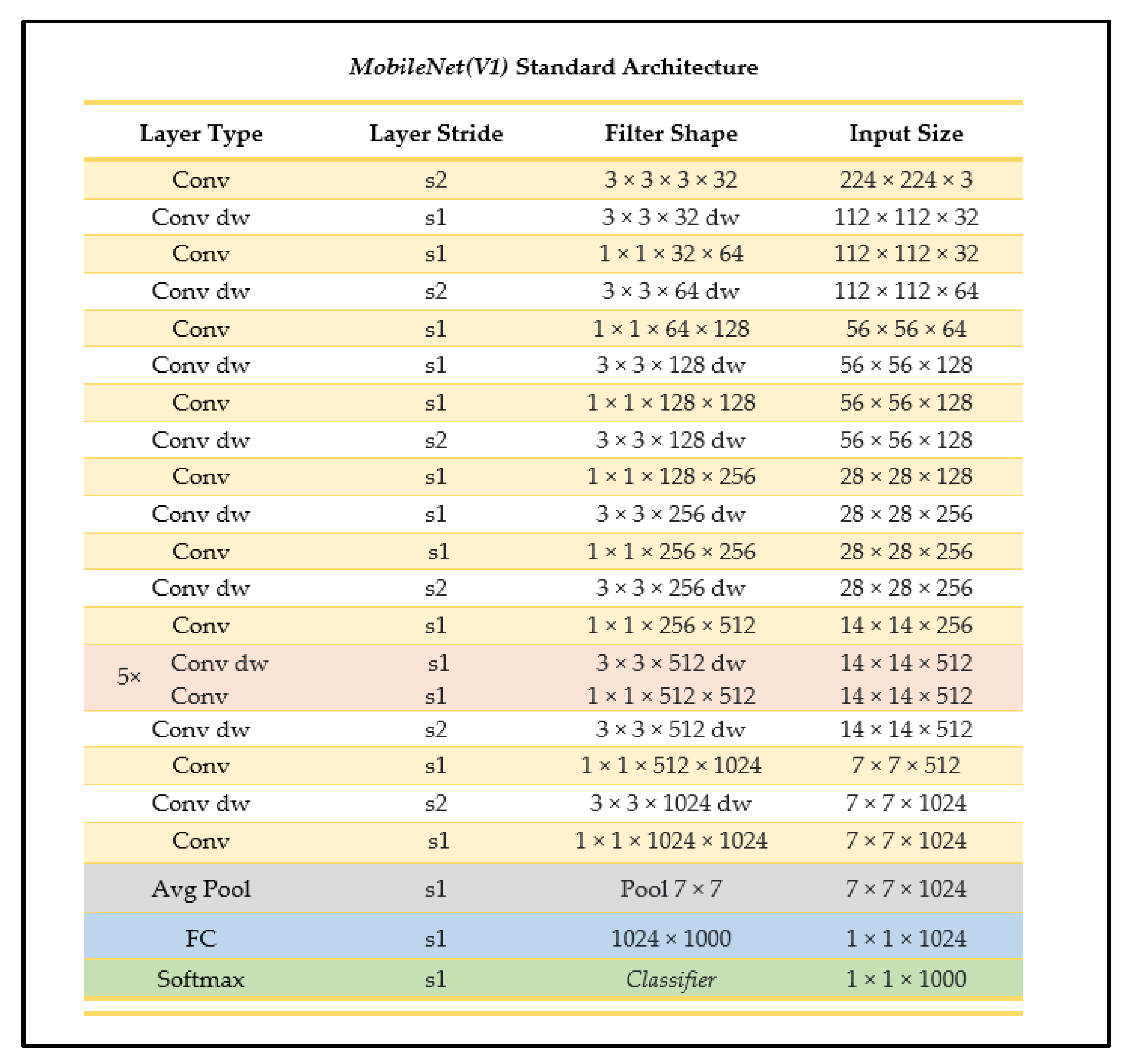
MobileNet is one of the main convolutional networks used when developing models for mobile device integration as it is a smaller-sized, high-accuracy, less-complex model with a well-supported integration process. The MobileNet CNN has two main parameters: the resolution multiplier and the width multiplier, using depthwise convolution followed by pointwise convolution processes for its architecture, with batch normalization and ReLU applied after every convolution layer [24] (see Figure 6). The depthwise separable convolutions approach used factorizes a standard convolution into a depthwise convolution and a pointwise (1 × 1) convolution, where the depthwise convolution applies a single filter to each input channel, and the pointwise convolution then applies a 1 × 1 convolution to combine the outputs of the depthwise convolution to generate the new features set [24]. A standard convolution uses one layer to filter and combine inputs whereas the depthwise separable convolution splits this process into two distinct, designated layers, making each layer more efficient.

2.4.2. MobileNetV2

MobileNetV2 is an enhanced neural network architecture from the MobileNet family tailored more specifically for computer vision in mobile and resource-constrained environments, designed to have improved efficiency and performance compared to its predecessor [25]. This CNN reduces memory by never fully using large tensors, reducing the need for main memory access [25]. MobileNetV2 builds on the MobileNetV1 architecture by using the efficient depthwise separable convolution approach and introducing two new architecture elements: linear bottlenecks between the layers, and shortcuts between the bottlenecks [25]. Figure 7 outlines the layered MobileNetV2 architecture.
Depending on the domain, MobileNetV2 could have a more promising performance than its predecessor as it can use half the number of operations, 30% fewer parameters, and smaller CPU runtime than its predecessor while achieving a higher accuracy on average [25]. For example, on ImageNet classification, MobileNetV2 seems to generally outperform its predecessor as seen in Figure 8, with fewer parameters and a smaller CPU runtime.
Based on the aforementioned qualities, we have decided to include MobileNetV2 as a part of our comparison to determine which MobileNet model would perform better for our dataset and application domain.

2.4.3. NasNetMobile

NasNetMobile is a convolutional neural network architecture that was designed to minimize computational complexity and achieve faster execution on mobile devices, allowing for parallel processing by using blocks of convolutional layers [26]. Released after MobileNetV2, it is considered a successor and an improvement that would allow for faster model processing without sacrificing accuracy, achieved by deviating from the standard sequential processing approach to instead rely on processing multiple layers in parallel using a blocks-and-strides architecture. Blocks are pre-defined network layers (considered as “outer skeletons”), and strides are subsets of each block that contain a variable of one to two layers [26]. The benefit of this strides’ architecture lies within the search algorithm adopted, as it allows the model to further partition layers to perform skips within the network, according to the filter size per layer, in turn more efficiently processing the layers to generate predictions [26].
The model architecture consists of a total of 769 layers, including an input layer, 371 convolutional layers, 188 activation layers, and 144 reduction layers, as well as incorporating global average pooling layers and batch normalization [26]. The model uses variant kernel sizes for its blocks, using both 3 × 3 and 5 × 5 kernels. These varying kernel sizes are unlike other models and help balance the diversity of layers to speed up the search algorithm. Figure 9 illustrates the visual architecture of NasNetMobile.

2.4.4. EfficientNet-B0

EfficientNet is one of the newest CNN model architectures recently developed. The CNN uses the method of uniform scaling for all the dimensions of the resolution, width, and depth of the network, using what is known as a compound coefficient (ϕ) [27]. In other neural networks, the alternative process used is performing a grid-search on the original small model when finding the optimal hyperparameters of a model. This means that, during the process of determining the coefficients of the depth, width, and resolution dimensions, if the network depth is increased by a certain number, then the same applies for the width and image resolutions, generating three different sets of coefficients. On the contrary, EfficientNet uses one main coefficient that has an established method of uniformly scaling the network in a fixed manner [27]. Figure 10 outlines the architectural stages of the EfficientNet-B0 network, a model belonging to the EfficientNet CNN family.
EfficientNet-B0 is one of the models provided in the EfficientNets family of models, and in its architecture is similar to MobileNetV2 and MNasNet in terms of having inverted residuals and linear bottleneck convolution, as well as excitation and squeeze blocks [27]. However, since EfficientNet-B0 has a faster floating-point operations per second (FLOPS) budget, it is slightly larger in size [27]. Figure 11 illustrates the layer breakdown of the EfficientNet model architecture.
The source dataset used to pre-train the EfficientNet-B0 model is the ImageNet dataset. Several studies have been conducted in order to test the efficiency of the EfficientNet-B0 model when executed both on its own and in comparison to other similar networks. One such study found that, when using different transfer learning methods and comparing the results of the EfficientNet-B0 model to other established pre-trained network models such as MNasNet, the EfficientNet-B0 model proved to achieve a better accuracy using less parameters [28]. Documented attempts of integrating an EfficientNet model into a mobile application have proven to result in very high accuracy scores for the model, using less parameters than some other common model types while also allowing the model to be scaled up effectively [27].

3. Experimental Results

We divided our results into two stages: preliminary results and post-preliminary results. For our preliminary results, we took a rudimentary approach with the optimization and evaluation of our models, where we used the base-line criteria to evaluate all 32 developed models, comparing the quantitative metrics of accuracy, precision, recall, F1-score, confusion matrices, ROC curves, and precision-recall curves. In the preliminary stage of the results analysis, we did not use k-fold cross-validation as it was computationally expensive to perform for all 32 models developed. The best four models were then selected (one per each network architecture) after a careful assessment of the evaluation scores. After comparing the best four models, K-fold cross-validation was performed only for the highest performing model so that a proper replicable evaluation of the model was ensured.
For reference, our results and their respective discussions use the following previously-established terms when differentiating between the developed models:
  • Referenced Hyperparameters: The base-line hyperparameters from [19], which include: learning rate = 0.01; epochs = 30; mini-batch size = 32; Adam optimizer; no regularization.
  • Proposed Hyperparameters: Our new optimized hyperparameters, which include: learning rate = 0.0001; epochs = 30, mini-batch size = 32; Adam optimizer; regularization with Dropout (0.5) technique.
  • Scenario 1: freezing 100% of base-network; no retraining.
  • Scenario 2: freezing first 80% of base-network; retrain last 20%.
  • Scenario 3: freezing first 50% of base-network; retrain last 50%.
  • Scenario 4: retraining entire base-network; no freezing.

3.1. Preliminary Results: Evaluation Metrics, Scenarios, and Hyperparameters

Across each of the four base network architectures (MobileNet, MobileNetV2, NasNetMobile, EfficientNetB0), we recorded evaluation metrics when varying the portions of the network that are retrained as well as when varying the standard hyperparameters used. Table 1, Table 2, Table 3 and Table 4 show the recorded evaluation metrics for accuracy, precision, recall, and F1-score.
Table 1 shows the evaluation metric results for the MobileNet models developed using the referenced hyperparameters from [19] and our proposed hyperparameters, tested per transfer learning scenario. The highest and lowest scores are 99% for all the proposed models’ scores, and 43% for the referenced Scenario 1 model’s accuracy score.
Table 2 shows the evaluation metric results for the MobileNetV2 models developed using the referenced hyperparameters from [19] and our proposed hyperparameters, tested per transfer learning scenario. The highest and lowest scores are 99% for the proposed Scenario 3 and 4 models’ scores, and 47% for the referenced Scenario 4 model’s F1-score.
Table 3 shows the evaluation metric results for the NasNetMobile models developed using the referenced hyperparameters from [19] and our proposed hyperparameters, tested per transfer learning scenario. The highest and lowest scores are 99% for the proposed Scenario 3 and 4 models’ scores, and 15% for the referenced Scenario 4 model’s F1-score.
Table 4 shows the evaluation metric results for the EfficientNetB0 models developed using the referenced hyperparameters from [19] and our proposed hyperparameters, tested per transfer learning scenario. The highest and lowest scores are 100% for all the proposed models’ scores, and 96% for the referenced Scenario 4 model’s accuracy, recall, and F1-scores.
The results in the tables above strongly indicate that our proposed hyperparameters yield better model performance and higher evaluation metrics than the referenced hyperparameters. Due to the nature and sizes of the target and source datasets, results also confirm that retraining only half the network (Scenario 3) seems to be, on average, most appropriate for the different network architectures and different hyperparameters tested.
Varying the network hyperparameters demonstrates clear effects on model performance. Improving and tweaking the choice of hyperparameters (proposed hyperparameters) seems to generally improve accuracy and evaluation scores of the individual models. Our proposed choice of hyperparameters—learning rate, mini batch-size, number of epochs, regularization (Dropout)—appear to demonstrably affect model performance positively and avoid more overfitting as opposed to the initial referenced hyperparameters.
Varying the transfer learning scenarios (the portions of the base networks that are retrained) also demonstrates clear effects on model performance. The ImageNet dataset that the base network architecture is trained on is very large in comparison to our target dataset, and does not specifically focus on the domain of diseased leaves; therefore, our dataset is considered to be much smaller in size and a different domain from the source dataset, indicating a theoretical performance improvement from retraining only half the network (Scenario 3). The effects of the hyperparameters and scenarios are further reviewed in Section 4.

3.2. Preliminary Results: Accuracy, Precision, Recall, and F1-Score Graphs

Figure 12 shows a graph charting the accuracy score results for all the trained models we developed, grouped based on the base-network architecture and hyperparameter variation used for the models. As can be seen in Figure 12, the accuracy scores vary across the base-network architectures, where we can see that the NasNetMobile models produced the worst accuracy scores, while the EfficientNetB0 models consistently perform the best in both hyperparameter variations.
The graph in Figure 13 shows the precision scores for all the models developed, which indicates close precision results between the EfficientNet (proposed parameters), MobileNet (proposed parameters), and MobileNetV2 (proposed parameters) models. However, the EfficientNet architecture proved to have the highest precision score overall, with a perfect 1.0 score. The model with the lowest precision score is NasNetMobile with the referenced hyperparameters with transfer learning Scenario 4.
Figure 14 showcases the recall scores of the models developed; those scores varied among the base-networks and the different transfer learning scenarios that were applied. The EfficientNet model with our proposed hyperparameters had a perfect recall score of 1.0, and it is also observed that the NasNetMobile models with the referenced hyperparameters had the lowest score, followed by the MobileNet model with Scenario 1 and referenced hyperparameters.
As observed from Figure 15, the NasNetMobile model with referenced hyperparameters proved to have the lowest F1-score with the Scenario 4 transfer learning method. Then this was followed by the MobileNet model’s first scenario implementation, which had an F1-score of 0.43. On the other hand, the EfficientNet architecture had a perfect F1-score across all transfer learning scenarios tested for our proposed hyperparameters, followed, at second-best, by the EfficientNet models with the referenced hyperparameters, then by the MobileNet models.

3.3. Best-of-Four Models

In order to compare model architectures against each other in more detail, we took the best four models, one per network architecture implemented, from the total 32 implemented models in order to compare them in post-preliminary results. Our findings executed on the PlantVillage dataset indicate the ranking from the worst- to best-performing network architecture, which are: MobileNetV2; NasNetMobile; MobileNet; EfficientNet. The average accuracies and F1-scores can be seen in Table 5.
The best model for each base network architecture we implemented is defined by three factors: the pre-trained base architecture; the transfer learning scenario (Sc. 1–4 from [20]) used; and the hyperparameter combination (original referenced parameters from [19] vs. our new proposed parameters) used.
We concluded that the best four models were the:
  • MobileNetV2 model with transfer learning Scenario 3 and the Proposed hyperparameters;
  • NasNetMobile model with transfer learning Scenario 3 and the Proposed hyperparameters;
  • MobileNet model with transfer learning Scenario 4 and the Proposed hyperparameters;
  • EfficientNetB0 model with transfer learning Scenario 4 and the Proposed hyperparameters.

3.4. Full 39 × 39 Confusion Matrices

Table 6 shows a small example of how our confusion matrix is represented for all of the 39 classes (only 4 classes are shown in the table for simplicity).
The confusion matrices are presented per model and are non-normalized in order to show the actual number of images in the held-out testing set being classified correctly.
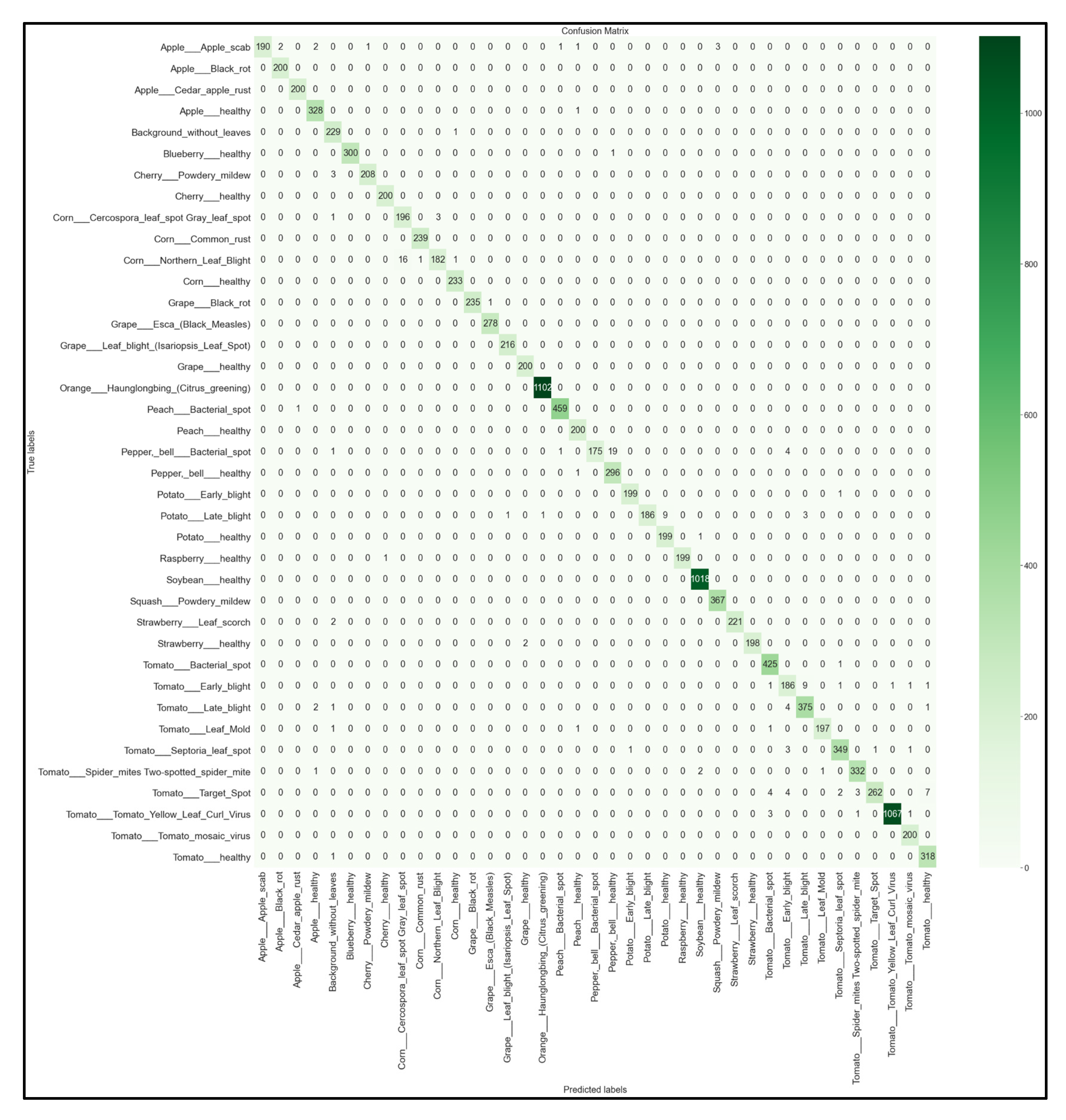
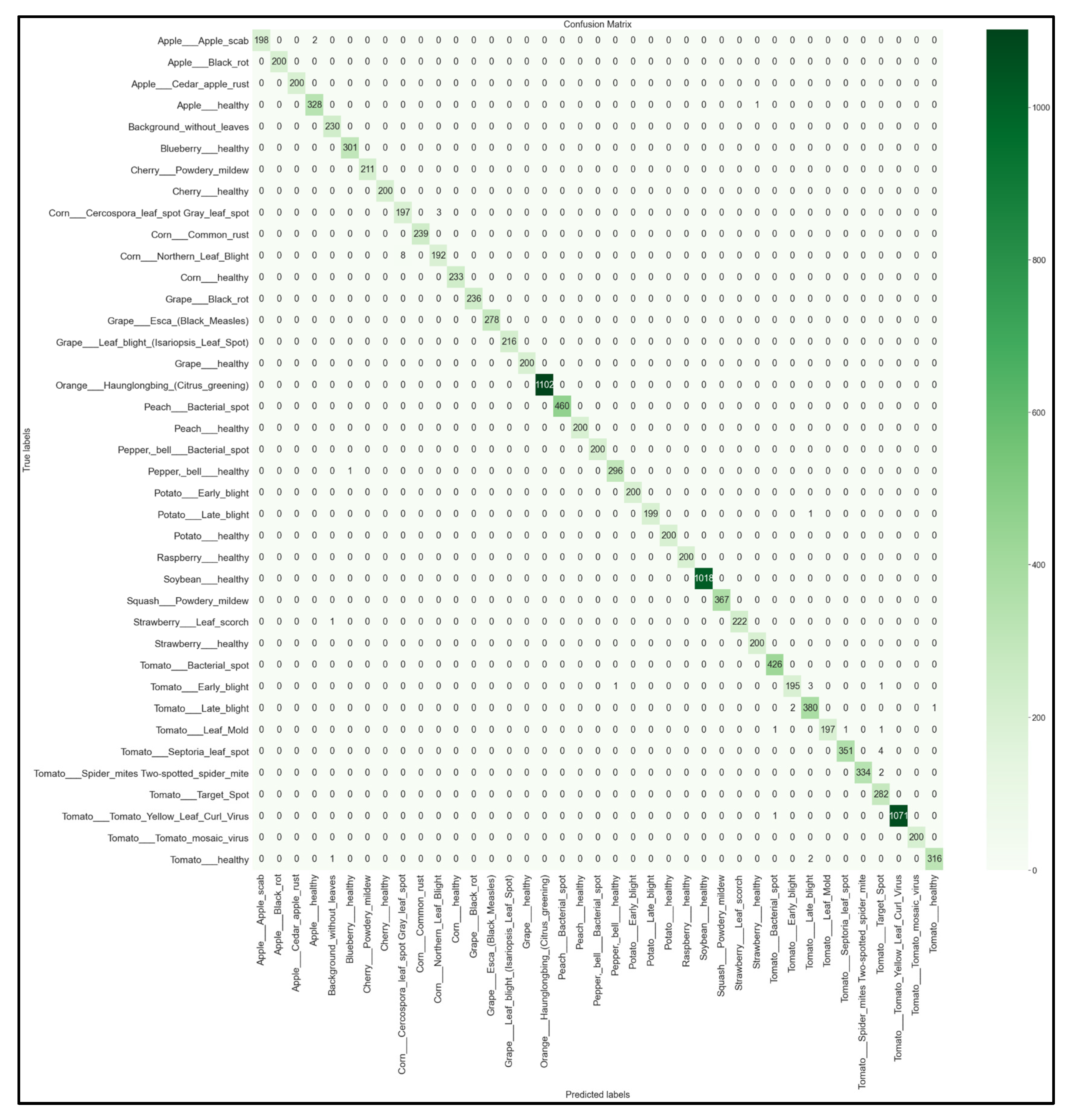
For each of the 32 models developed, we obtained the multi-class 39 × 39 confusion matrix on the held-out testing set (total of 12,313 images). The confusion matrices for each of the best-performing models per network architecture (MobileNet, MobileNetV2, EfficientNetB0, NasNetMobile) are shown below in Figure 16, Figure 17, Figure 18 and Figure 19.
Looking at the 39 × 39 confusion matrix figures for each network, we see the NasNetMobile model produced a maximum of 32 misclassifications, while the MobileNetV2 model maxed out at 19 misclassifications, making them the worst-performing models out of the four networks above. Meanwhile, the better-performing MobileNet model maxed out at 12 misclassifications, and the EfficientNetB0 model achieved the fewest misclassifications, reaching a maximum of 8 misclassifications for Corn_Northern_Leaf_Blight (out of 200 images).
As the confusion matrix is one of the most prominent indicators of a model’s overall performance across its supported classes, it can be concluded that EfficientNetB0 outperformed the rest of the models based on the 39 × 39 confusion matrices.

3.5. ROC Curves

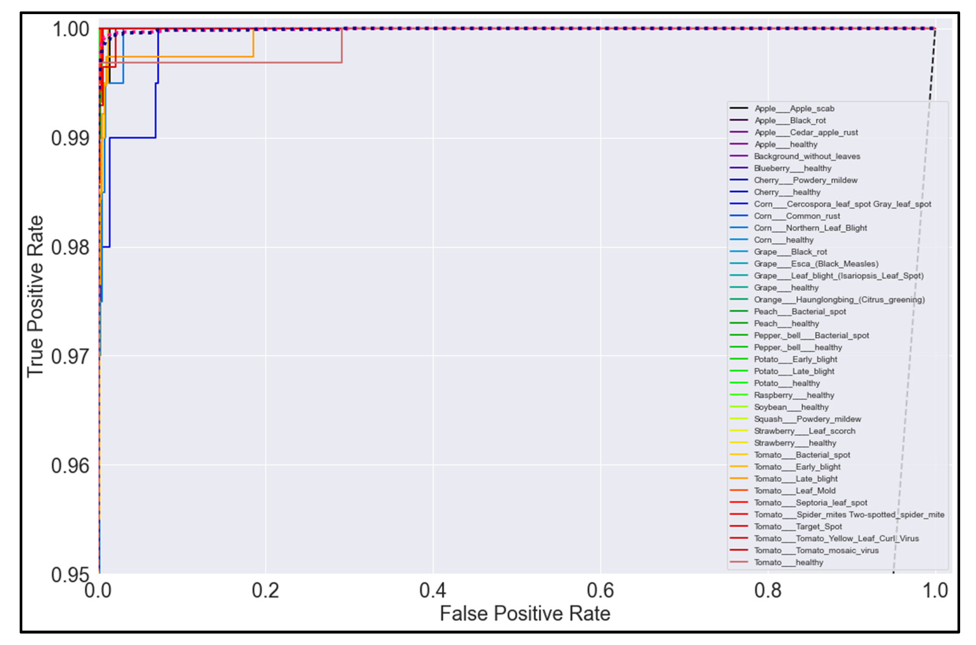
Figure 20, Figure 21, Figure 22 and Figure 23 show the ROC curves for the four best-performing models per network architecture implemented.
On initial inspection of the figures, all the models appear to perform well overall; therefore, we must zoom in further to see clearer performance details in the ROC curves. Based on the figures above, we can see that, between the curves of the four different models, the MobileNet and EfficientNetB0 models outperformed the NasNetMobile and MobileNetV2 models—the ROC curves are evaluated by considering that the closer the curves of each class are to the top-left corner of the graph, the better the ROC evaluation and the better the model performance.

3.6. Post-Preliminary Results

After comparing the various evaluation metrics between each of the best four models, the EfficientNetB0 model with transfer learning Scenario 4 and our proposed hyperparameters was selected as the best-performing model. This is due to the EfficientNetB0 model obtaining the highest accuracy and F1-scores. As seen in its 39 × 39 confusion matrix (Figure 19), this model rarely makes false predictions across all classes. Although there exists a small class imbalance in parts of the dataset—which was reflected in the image counts from the testing subset (Figure 5)—the heatmap shows that the EfficientNetB0 model performs very well regardless of the class image counts. The highest false prediction count for this model maxed out at 4 incorrectly predicted images out of 282 tested images, which were attributed to the Tomato_Septora_Leaf_Spot disease being mistaken for the similar-looking Tomato_Target_Spot disease (although the plant species was still correctly identified in these false predictions). The reported accuracy, precision, recall, and F1-score for the EfficientNetB0 model all obtained 100% on the held-out test set without any detectable overfitting. Therefore, the EfficientNetB0 model clearly outperformed the other architectures and thus is the model best suited for our needs for our mobile solution development.
Since we used the Hold-Out method for the preliminary comparisons, and there is a possibility of coincidentally obtaining a good data split using this method, a K-Fold Cross-Validation was then performed to ensure the performance of the best model (the EfficientNetB0 model with Sc. 3 and proposed hyperparameters).

3.7. K-Fold Cross Validation

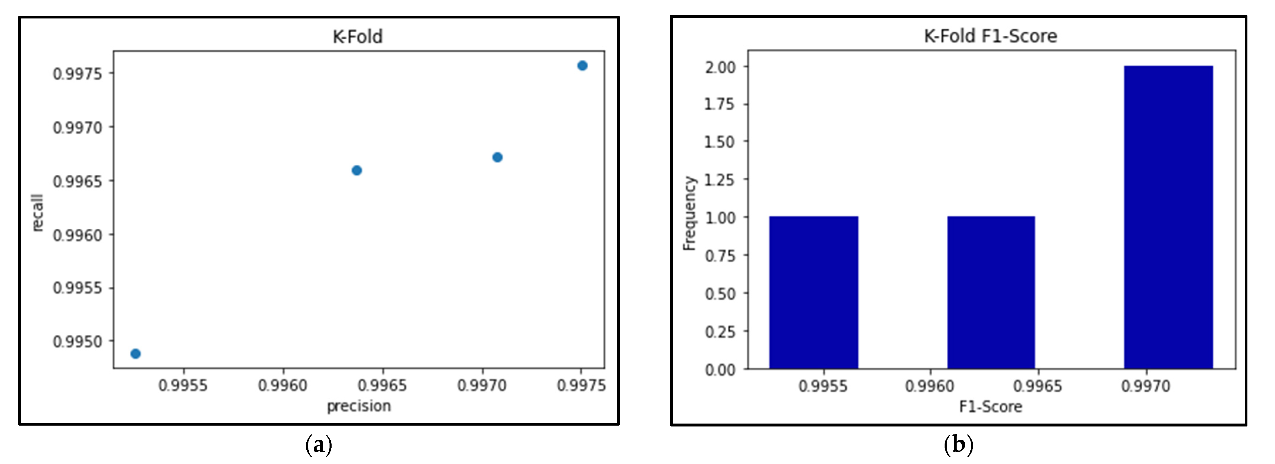
Figure 24a shows the precision-recall results for the best-performing EfficientNetB0 model’s 4-fold Cross Validation, and Figure 24b shows the respective F1-scores for each fold. Meanwhile, Table 7, Table 8 and Table 9 break down the F1-score, precision score, and recall score for each fold, as well as the mean and standard deviation of the respective scores.
As seen in Table 7, Table 8 and Table 9, the F1-score of the EfficientNetB0 model slightly decreased to an average of 99.65%, when the same model had previously scored an average of 100% using the Hold-out method. This is because the K-Fold Cross-Validation method can often provide a better estimate of how a model performs when it takes the averages of different folds in the data, thereby maximizing the use of the data and avoiding any potential bias of ‘lucky’ data splits. Therefore, because of these k-fold results, we can be confident that this model will perform well even with different splits of data.

4. Discussion

As seen in the evaluation of our preliminary results, we visualized the accuracy, precision, recall, and F1-scores so that we could observe the trends that occur across our implemented architectures, scenarios, and hyperparameters.
Overall, the best-performing model for our domain was concluded to be the fully retrained EfficientNetB0 base network (trained using the transfer learning Scenario 4 approach) using our improved proposed hyperparameters. This model had the most consistent top performance across our evaluated metrics, and these performance results were further supported by our K-fold cross validation evaluation, ensuring that the model confidently performed well with no data-split biases.
Beyond trying to find the best-performing model for the solution domain, our project also aimed to investigate the effects of using different CNN architectures, the effects of varying the retrained portions of the base networks, and the effects of varying the network hyperparameters on the models’ performances.
When investigating the effects of using different CNN architectures as the base-networks of our models, our findings show that the EfficientNetB0 model architecture frequently outperformed the MobileNetV2, MobileNet, and NasNetMobile models when considering the average scores and confusion matrices. The order of best- to worst-performing architectures were: EfficientNet; MobilNet; NasNetMobile; MobileNetV2.
When investigating the effects of varying the retrained portions of the base networks (i.e., varying the transfer learning scenarios used), we observed that, across all the models, Scenario 3 showed the best performance on average. This is evident as it never dropped below 67% for both the accuracy and F1-scores, and was always either the highest scoring or within 1% off the highest scoring model. This aligns with what we expected from a theoretical standpoint, as, according to [20], Scenario 3 (freezing the first half of the neural network and retraining the other half) is most useful when you have a target dataset that is smaller and of a relatively different domain to the pre-trained dataset. While the ImageNet dataset that the base-network architecture is trained on includes millions of images and contains some images of plants and leaves, these images are not specifically of classified, close-up, diseased leaves, which means our dataset is considered to be of a relatively different domain and substantially smaller in size than the pre-trained source dataset, in turn falling within the recommended conditions of using Scenario 3. On average, Scenario 4 seems to trend as the worst-performing transfer learning scenario. This may be due to overfitting, as using a smaller dataset to fine-tune the entire base-network is often prone to overfitting the developed model as it becomes less able to generalize its learned features to new data. Meanwhile, our results show that Scenario 2 performed better than Scenario 1. This may be due to the difference in size between the pre-trained source dataset and our PlantVillage dataset and how these sizes factor into the transfer learning scenarios.
When investigating the effects of varying the network hyperparameters on the models’ performances, our results show that our proposed choice of hyperparameters—the learning rate, mini batch-size, and number of epochs—greatly improved the classification accuracy of the models. Using a smaller learning rate significantly improved results in comparison with initial results from [19]. Additionally, our use of Dropout layers for regularization helped avoid overfitting in the models, in contrast with some observed overfitting when using the initial (referenced) hyperparameters from [19]. By observing the difference between training and validation accuracies and losses, we can conclude that our models that used the proposed hyperparameters were able to better generalize the learned features for new, unseen data. As such, we have achieved our intended goal of improving on the referenced models developed in [19].
Our results indicate that the performance of the model depends on the model architecture and hyperparameters chosen as well as the portion of the network trained. Therefore, we have found that all three hypothesized factors (the model architecture, hyperparameter optimization, and the portion of the network retrained) can all each have a significant effect on the model performance.

5. Integrated System Implementation

To create our proposed mobile plant care support system for novice gardeners, we designed a simple-yet-comprehensive, three-tier solution consisting of a mobile application, a backend cloud database, and the aforementioned best-performing classification model. To maintain the desired lightweight portability and ease-of-access requirements of our system, we decided that an Android-based mobile application would be our primary touchpoint for the system, and that users would access all our implemented functionalities directly through the application. Our backend database was developed using Cloud Firestore to keep the system’s user-wide data stored in a centralized and secure fashion while simultaneously allowing for instances of user-specific data to also be stored and accessed using a similar backend process in the application. The mobile application is integrated with the respective deep learning classification model using a TensorFlow Lite file format and with the cloud database using the Cloud Firestore SDKs available for Android development. We chose to name the mobile app system “AgroAId” to present a clear and easy name that encompasses the system’s core values of agriculture, artificial intelligence (AI), identification, and plant care assistance (aid) in a unique, innovative, and simple manner.

5.1. Mobile Application Functionalities

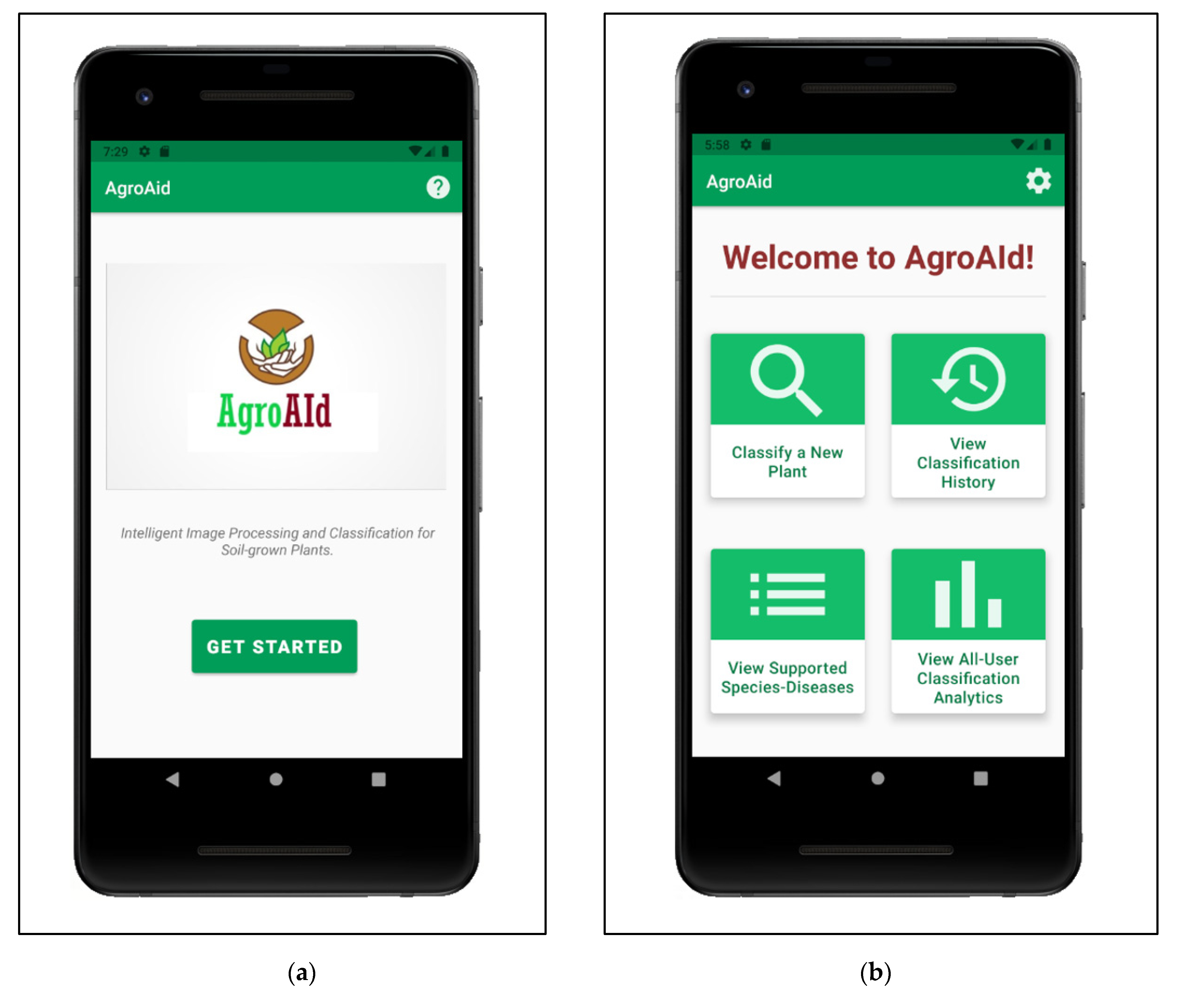
Maintaining a simple standard interface, the mobile application starts up on a minimal home page (Figure 25a) that leads the user to a central activity (Figure 25b) from which they can then access all the main system functionalities. The functionalities implemented in our system include:
  • Classifying a new input plant image based on the visual characteristics of its [species–disease] combination;
  • Retrieving and presenting the corresponding plant care details (e.g., symptoms and treatments) for the particular [species–disease] combination identified in an input image;
  • Storing and presenting a user-specific classification history;
  • Retrieving and presenting a list of all [species–disease] combinations supported by the system;
  • Configuring custom user settings pertaining to the user’s classification history and location region;
  • Retrieving and presenting user-wide spatiotemporal analytics about the system’s most commonly identified [species–disease] combinations filtered by season and region.
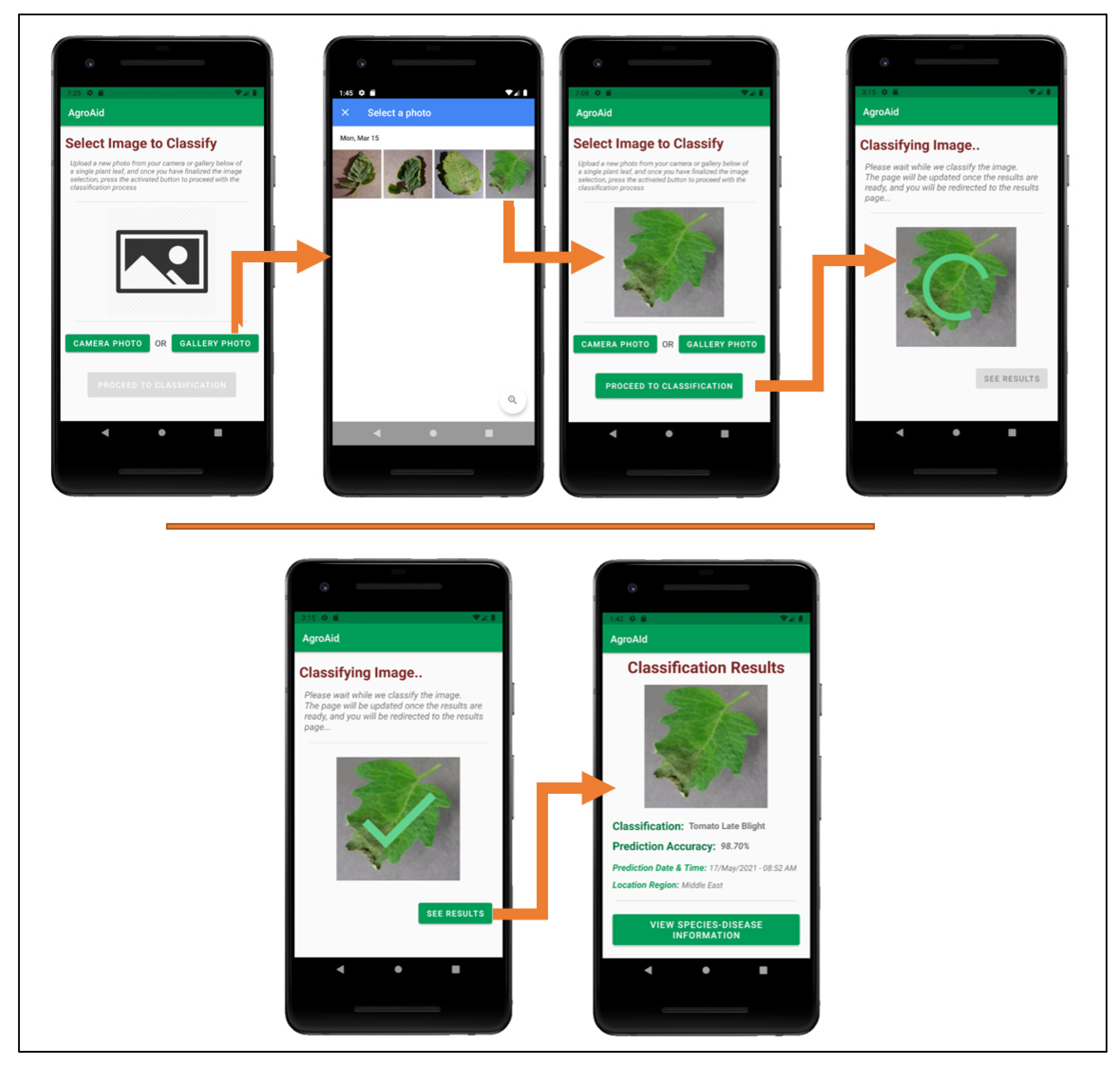
Figure 26 illustrates a walkthrough of the image classification functionality provided by our plant care support system as the user would experience it. The system’s classification functionality is initiated when the user selects to “Classify a New Plant” from the central activity in Figure 26. From there, the user is directed to an image selection activity, where they can choose to input an image either using the device’s camera (i.e., taking a new photo) or the device’s gallery (i.e., uploading an existing stored image). Once the user confirms their selected image, an intermittent loading activity is displayed while the input image is classified in the background by the integrated deep learning model. Upon completing the classification, the results are displayed to the user in a dedicated results screen containing the classified image, predicted class label, prediction accuracy (confidence level), date and time of the classification, and the location region in which the user conducted the classification. The classification results are then stored in the system’s database under the user’s personal classification history, and the user-wide analytics are updated with the details of the identified class, location region, and season. The results screen also gives the user the choice to explore more plant-care information about the identified [species–disease] combination.
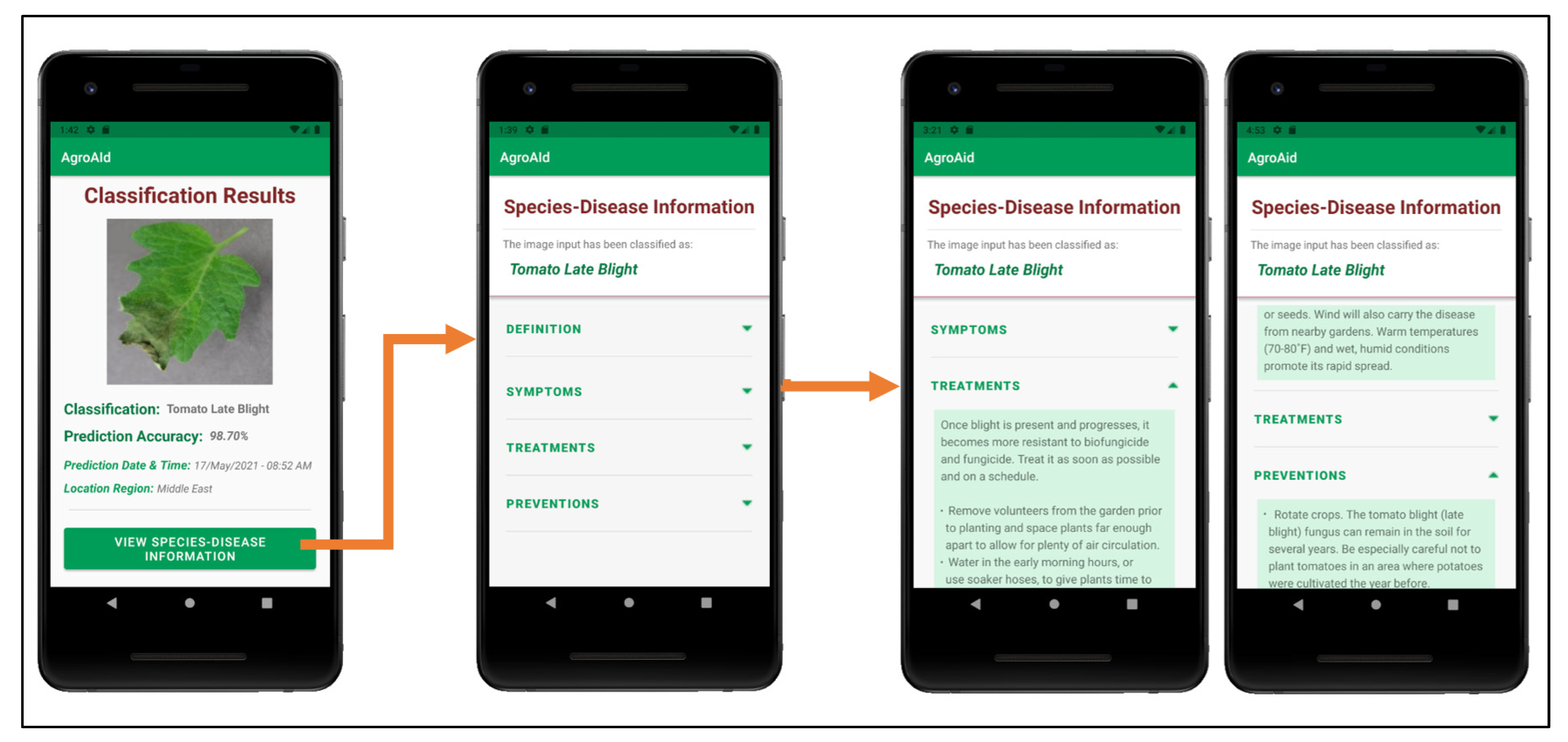
Figure 27 shows an example of the additional plant care support details provided to a user upon receiving a classification result; these details include the disease definition, symptoms, treatments, and future prevention for the particular [species–disease] combination identified. The plant care details were collected for every [species–disease] combination recognized by the system to ensure that the user is provided with useful and accurate expert horticultural information for all of the system’s supported classification results. The information is stored in the centralized backend database to be accessible to all users and the details for the specific combination of interest are loaded in once the Species–Disease Information activity is triggered via a call to the designated class responsible for all database operations. It is emphasized that the information presented is specific to the species-and-disease combination as the same disease can have different symptoms or treatments depending on the species affected—this is a common, major pitfall that novice gardeners often face because they often do not possess the expert knowledge about the characteristics of particular species-and-disease combinations to know how to specifically treat them. As such, our application aims to provide the necessary information to guide gardeners to use plant care methods that are appropriate to the particular species and disease at hand in an attempt to make the plant care process easier and more effective.
A user can view a full list of all the [species–disease] combinations supported by the system from the central activity (Figure 25b)—the supported combinations are those that the integrated AI model is able to recognize and classify. Having this feature available to users is necessary as the integrated model cannot identify all possible existing [species–disease] combinations, meaning that an error in classifying an unsupported image is plausible. Therefore, presenting the list allows users to check if the plant species they wish to classify is supported and can minimize or help clarify any incorrect classifications that may occur as a result of inputting an image of an unsupported species/disease (see Figure 28).
As the user continues to generate classification results using the system, they will accumulate their own collection of classification history records, which are stored in a user-specific sector of the system’s backend database and can be accessed by the user from the central activity (Figure 25b). The Classification History activity, as demonstrated in Figure 29, lists the user’s past classification results chronologically from most-to-least recently classified and includes an initial preview of each record, including an icon-sized version of the classified image, the predicted class, the prediction accuracy, and the date and time of the classification. Each record card can then be expanded to see the full classification results page, and from there the user can optionally re-access the plant care information for that particular classification result, allowing them to refer back to the details at any time. The Classification History activity also includes a distinguished minimizable card above the history records that displays the user’s most frequently classified [species–disease] combination based on their classification history—this statistic can be useful for gardeners to learn if there is a particularly prominent common issue they are facing among their plants and as such allow them to seek a broader solution for treating it.
Custom app settings were developed for the system to allow users to flexibly configure their classification history and their location region (see Figure 30). Users can select the maximum number of records they wish to see in their classification history list and the region from which they are conducting their classifications, the values of which are saved locally to the user’s device. The selected location region is used (along with the date and time of a classification) to update the system’s global analytics collection for each new classification result generated by a user.
A unique feature included in our system is its ability to generate and present user-wide spatiotemporal analytics based on the users’ collective classification results—by considering the predicted class label, date, and location region of each classification conducted using our system, we can present the top, most commonly classified [species–disease] combinations filtered by region and season.
The data is stored in a dedicated centralized collection in the database that tallies the total count of classifications conducted with respect to their region, season, and identified [species–disease] combination. This global statistical data can be incredibly beneficial to gardeners to help them better understand the agricultural patterns that occur around them and how these external environmental or seasonal factors may be affecting their plants, in addition to generating new useful data about global agricultural trends that could then be used for future research in the field.
Within the application, users can access these analytics from the central activity, where they are directed to a screen that contains two drop-down filters to select the region and season of interest (see Figure 31). Once the filters are selected and confirmed, the requested analytics are retrieved from the centralized backend database and the top 5 most commonly classified [species–disease] combinations for the selected region and season are returned and displayed in the Analytics activity.
Beyond the textual results, the system also provides users the options to generate bar and pie charts of the analytics as an additional visualization of the statistics. Figure 32 illustrates the respective bar and pie charts generated by the system for the same spatiotemporal analytics retrieved in Figure 31. The open-source MPAndroidChart library was used to create the base of the interactive chart views displayed in the application.

5.2. Database Implementation and Integration

To implement the backend database component, a Cloud Firestore database was created to meet the requirements of storing both user-specific and centralized data, and the need for querying the data efficiently.
Figure 33 is a visual representation of the schema implemented for our Firestore database and illustrates how our database stores our four main categories of information in designated top-level collections, including:
  • A collection for the user-specific classification histories;
  • A collection for the user-wide classification analytics;
  • A centralized collection for the [species–disease] combinations supported by the system;
  • A centralized collection for the detailed plant-care information for each supported [species–disease] combination.
Documents and subcollections were then used within these collections to achieve the desired hierarchical storage structure and to take advantage of Firestore’s query-oriented nature. No personal information is stored about the users in the system—instead, a ‘user’ is defined by the unique application instance they are using, and the system collects and organizes the classification histories based on that unique ID.
The Cloud Firestore database was fully integrated into the system’s Android mobile application by addressing four main areas of integration:
  • Integrating the Cloud Firestore SDKs, plugins, and dependencies into the development environment;
  • Initializing Cloud Firestore within the application using an object instance;
  • Enabling the addition of new data to the database from within the application;
  • Enabling the retrieval of data from the database from within the application.
To maintain a modular design in our system application, a separate Java class was created and designated for all database-related functionalities, including connecting to the database, performing read queries, and writing new data. All application activities that require access to the database for storing new data or retrieving existing data execute the desired operations through an instantiated DatabaseConnector object’s class methods. For modularity and ease of execution, a dedicated class function was created to represent the full process of each system operation (e.g., writing a new history record; reading in all system-supported species and diseases; retrieving a classification history; requesting classification analytics). Some custom object classes were also created within the application to simplify the process of handling the more complex database records when reading and writing data in the system (e.g., for handling all components of a classification result record in a single class object).

5.3. Deep-Learning Model Conversion and Integration

To be able to run AI models on a mobile device, the original AI model files developed must first be converted into TensorFlow Lite files. The TensorFlow Lite framework was used as it is specifically designed for the on-device execution of deep learning models, storing the models in a special reduced file format that allows for efficient execution rates while using limited computing and memory resources [29]. Following standard convention, the Python TFLiteConverter API class is used to convert the AI model file into a FlatBuffer tflite file [30].
The process of executing a trained model on a device to generate predictions is known as inference and can be achieved on a mobile device using an Interpreter object. Specifically, the TensorFlow Lite Interpreter library was used to run inference on the client devices when using TFLite files for our Java-developed Android application, and the corresponding Java API and Android support libraries and dependencies were used to manage the model assets in our system.
Below is the general four-step process we used to run TensorFlow Lite inference and generate our model predictions in our mobile application system:
  • Load the TFLite deep learning model and its corresponding labels into the application memory;
  • Transform the received raw input data (the image selected to classify) into the required format to be compatible with the integrated deep learning model;
  • Run inference, i.e., use the TensorFlow Lite API to execute the classification model for the given new input and generate tensor outputs;
  • Interpret the tensor outputs to present meaningful results to the end-user (in our case, the classification results of the input image).
This four-step process allows our system to successfully access and execute the integrated AI classification model on the user-input plant images. For modularity and ease of execution, a single Java class was used for all AI model-related functions, where dedicated class functions generally map to each of the four steps outlined above so that a single Classifier object can be instantiated to load the model, preprocess the user-input image, execute the classification model on the new image, and generate the desired classification results in a format presentable to the user.
The data transformation and results interpretation steps of the outlined inference process (steps 2 and 4) can often vary depending on the specific model requirements and system domain. In our case, the data transformation step involves preprocessing the user-input image by resizing it to the integrated model’s required input size, as well as normalizing the image pixels, and converting the bitmap image to a byte buffer. The tensor outputs returned by our system’s AI model are the prediction confidence percentages for each class recognized by the model (39 values in total). As such, the output interpretation step in our case involves mapping this returned list of probabilities to the list of class labels recognized by the model and sorting the paired list elements by their confidence percentages to determine the class label that has the highest prediction accuracy for the given input image. The details of the prediction result with the highest probability are then returned to be displayed to the user as the final classification result of their input image.

6. Conclusions

This research project proposed a system that aims to assist novice gardeners and small-scale farmers to classify the [species-and-diseases] combinations of their plants non-invasively by inputting an image of a single plant leaf into the system and producing a classification result based on the image. Additionally, the system provided further support by outlining the plant care details for the identified [species–disease] combination, including the symptoms, treatments, and future preventions. The goal is to help novice gardeners avoid the major, common pitfall of misidentifying or mistreating a particular [species–disease] combination as a result of their lack of expert agricultural knowledge, and to in turn provide an efficient and more sustained plant care approach. We developed several pre-trained CNNs and compared them against each other to evaluate which model achieved optimum performance. We began the evaluation with a rudimentary approach to compare the effects of the base architectures, transfer learning scenarios, and hyperparameters, then further assessed the top performing models for each unique architecture used to determine the best-performing model across the board of metrics. The best performing model selected from the model comparison process was then integrated into the mobile app system solution, made accessible to the users through the mobile application touchpoint. The application logic and database were structured to try and maintain a modular design across all classes and to optimize the querying processes executed within the system. Beyond the user-specific classification and plant care functionalities, we also added the user-wide analytics functionality to generate a new spatiotemporal dataset that illustrates the common [species–disease] combination trends filtered by region and season. The trends analysis and graphing features were available to all users of the system, encouraging them to expand their agricultural knowledge and to investigate how their plant trends may relate to local and global patterns.
Our findings show that the EfficientNetB0 network outperformed MobileNetV2, MobileNet, and NasNetMobile when considering average scores and confusion matrices. Our best-performing model was found to be a fully retrained EfficientNetB0 base network (Scenario 4) with improved hyperparameters. Beyond trying to find the best-performing model for the solution domain, our project also aimed to investigate the effects of varying the retrained portions of the base networks (transfer learning scenario), the effects of using different CNN architectures, and the effects of varying the network hyperparameters on the models’ performances. Our model analysis results concluded that varying the percentage of convolutional layers retrained for the base networks does impact the model performance, indicating that, on average, there was a trend of Scenario 3 performing the best for the given PlantVillage dataset and solution domain. We have found that the model architecture, hyperparameter optimization, and the portion of the network retrained can all each have a significant effect on the model performance, and that understanding the most suitable portion of the network to retrain can save time and computational effort when training models using a transfer learning approach, especially for pre-trained models that have deep and complex architectures.

Future Work

One of the biggest challenges in solving agricultural problems using artificial intelligence approaches is the lack of available natural large-scale data. Although the PlantVillage dataset is one of the largest and most comprehensive datasets available for plant disease classification problems, many public plant image datasets are specialized for laboratory settings under artificial lighting rather than natural settings, which means that their training results may not reflect their true performance in the expected natural environmental conditions. Therefore, a potential significant future expansion for our project would be to use some of the higher-accuracy user inputs collected by our system in natural settings to expand our initial dataset by retraining the integrated model using a semi-supervised learning approach. Potential expansions to the system functionalities could include integrating more plant knowledge support features to further assist novice gardeners, such as including contacts to local experts or creating a social community aspect to allow users to communicate and share advice on gardening and farming, moving the system towards serving as a one-of-a-kind central platform for all plant disease and care needs. Finally, we hope the new spatiotemporal analytics data we have generated within our system encourages future work on investigating global and seasonal [species–disease] classification trends.

Author Contributions

Conceptualization, R.S., S.A., Y.R., and M.R.; methodology, S.A. and M.R.; software, M.R. and R.S.; validation, S.A. and Y.R.; formal analysis, R.S. and Y.R.; data curation, Y.R. and R.S.; writing—original draft preparation, M.R., S.A., Y.R. and R.S.; writing—review and editing, T.S., S.A. and M.R.; visualization, M.R. and R.S.; supervision, T.S.; project administration, T.S.; funding acquisition, Y.R. and S.A. All authors have read and agreed to the published version of the manuscript.

Funding

This research was supported in part by the American University of Sharjah, grant number URG21-001. This work is also supported in part by the Open Access Program from the American University of Sharjah. This paper represents the opinions of the authors and does not mean to represent the position or opinions of the American University of Sharjah.

Institutional Review Board Statement

Not applicable.

Informed Consent Statement

Not applicable.

Data Availability Statement

A publicly available augmented dataset was used in this study. This data can be found openly on Mendeley Data at https://doi.org/10.17632/tywbtsjrjv.1 (accessed on 20 May 2022).

Conflicts of Interest

The authors declare no conflict of interest. The funders had no role in the design of the study; in the collection, analyses, or interpretation of data; in the writing of the manuscript; or in the decision to publish the results.

References

  1. Lu, J.; Tan, L.; Jiang, H. Review on convolutional neural network (CNN) applied to plant leaf disease classification. Agriculture 2021, 11, 707. [Google Scholar] [CrossRef]
  2. Ahmad, M.; Abdullah, M.; Moon, H.; Han, D. Plant disease detection in imbalanced datasets using efficient convolutional neural networks with stepwise transfer learning. IEEE Access 2021, 9, 140565–140580. [Google Scholar] [CrossRef]
  3. O’Mahony, N.; Campbell, S.; Carvalho, A.; Harapanahalli, S.; Hernandez, G.V.; Krpalkova, L.; Riordan, D.; Walsh, J. Deep learning vs. traditional computer vision. Adv. Intell. Syst. Comput. 2019, 943, 128–144. [Google Scholar] [CrossRef] [Green Version]
  4. Elsayed, E.; Aly, M. Hybrid between ontology and quantum particle swarm optimization for segmenting noisy plant disease image Int. J. Syst. Appl. Eng. Dev. 2020, 14, 71–80. [Google Scholar] [CrossRef]
  5. Asefpour Vakilian, K.; Massah, J. An artificial neural network approach to identify fungal diseases of cucumber (Cucumis sativus L.) plants using digital image processing. Arch. Phytopathol. PlantProt. 2013, 46, 1580–1588. [Google Scholar] [CrossRef]
  6. Yang, J.; Bagavathiannan, M.; Wang, Y.; Chen, Y.; Yu, J. A comparative evaluation of convolutional neural networks, training image sizes, and deep learning optimizers for weed detection in Alfalfa. Weed Technol. 2022, 1–30. [Google Scholar] [CrossRef]
  7. Shaji, A.P.; Hemalatha, S. Data augmentation for improving rice leaf disease classification on residual network architecture. Int. Conf. Adv. Comput. Commun. Appl. Inform. (ACCAI) 2022, 1–7. [Google Scholar] [CrossRef]
  8. Chen, J.; Chen, W.; Zeb, A.; Yang, S.; Zhang, D. Lightweight inception networks for the recognition and detection of rice plant diseases. IEEE Sens. J. 2022, 22, 14628–14638. [Google Scholar] [CrossRef]
  9. Liu, J.; Wang, X. Early recognition of tomato gray leaf spot disease based on MobileNetv2-YOLOv3 model. Plant. Methods 2020, 16. [Google Scholar] [CrossRef]
  10. Ma, J.; Du, K.; Zheng, F.; Zhang, L.; Gong, Z.; Sun, Z. A recognition method for cucumber diseases using leaf symptom images based on deep convolutional neural network. Comput. Electron. Agric. 2018, 154, 18–24. [Google Scholar] [CrossRef]
  11. Sagar, A.; Dheeba, J. On using transfer learning for plant disease detection. bioRxiv 2020. [Google Scholar] [CrossRef]
  12. Altuntaş, Y.; Kocamaz, F. Deep feature extraction for detection of tomato plant diseases and pests based on leaf images. Celal Bayar Üniv. Fen Bilim. Derg. 2021, 17, 145–157. [Google Scholar] [CrossRef]
  13. Rao, D.S.; Babu Ch, R.; Kiran, V.S.; Rajasekhar, N.; Srinivas, K.; Akshay, P.S.; Mohan, G.S.; Bharadwaj, B.L. Plant disease classification using deep bilinear CNN. Intell. Autom. Soft Comput. 2022, 31, 161–176. [Google Scholar] [CrossRef]
  14. Dammavalam, S.R.; Challagundla, R.B.; Kiran, V.S.; Nuvvusetty, R.; Baru, L.B.; Boddeda, R.; Kanumolu, S.V. Leaf image classification with the aid of transfer learning: A deep learning approach. Curr. Chin. Comput. Sci. 2021, 1, 61–76. [Google Scholar] [CrossRef]
  15. Chethan, K.S.; Donepudi, S.; Supreeth, H.V.; Maani, V.D. Mobile application for classification of plant leaf diseases using image processing and neural networks. Data Intell. Cogn. Inform. 2021, 287–306. [Google Scholar] [CrossRef]
  16. Valdoria, J.C.; Caballeo, A.R.; Fernandez, B.I.D.; Condino, J.M.M. iDahon: An Android based terrestrial plant disease detection mobile application through digital image processing using deep learning neural network algorithm. In Proceedings of the 2019 4th International Conference on Information Technology (InCIT), Bangkok, Thailand, 24–25 October 2019. [Google Scholar]
  17. Ahmad, J.; Jan, B.; Farman, H.; Ahmad, W.; Ullah, A. Disease detection in plum using convolutional neural network under true field conditions. Sensors 2020, 20, 5569. [Google Scholar] [CrossRef]
  18. Reda, M.; Suwwan, R.; Alkafri, S.; Rashed, Y.; Shanableh, T. A mobile-based novice agriculturalist plant care support system: Classifying plant diseases using deep learning. In Proceedings of the 2021 12th International Conference on Information and Communication Systems (ICICS), Valencia, Spain, 24–26 May 2021. [Google Scholar]
  19. Syamsuri, B.; Negara, I. Plant disease classification using Lite pretrained deep convolutional neural network on Android mobile device. Int. J. Innov. Technol. Explor. Eng. 2019, 9, 2796–2804. [Google Scholar] [CrossRef]
  20. Elgendy, M. Deep Learning for Vision Systems; Manning Publications: Shelter Island, NY, USA, 2020; pp. 240–262. [Google Scholar]
  21. Zhuang, F.; Qi, Z.; Duan, K.; Xi, D.; Zhu, Y.; Zhu, H.; Xiong, H.; He, Q. A comprehensive survey on transfer learning. Proc. IEEE 2021, 109, 43–76. [Google Scholar] [CrossRef]
  22. Barbedo, J.G.A. Impact of dataset size and variety on the effectiveness of deep learning and transfer learning for plant disease classification. Comput. Electron. Agric. 2018, 153, 46–53. [Google Scholar] [CrossRef]
  23. Geetharamani, G.; Arun Pandian, J. Identification of plant leaf diseases using a 9-layer deep convolutional neural network. Comput. Electr. Eng. 2019, 76, 323–338. [Google Scholar] [CrossRef]
  24. Howard, A.G.; Zhu, M.; Chen, B.; Kalenichenko, D.; Wang, W.; Weyand, T.; Andreetto, M.; Adam, H. Mobilenets: Efficient convolutional neural networks for mobile vision applications. arXiv 2017. [Google Scholar] [CrossRef]
  25. Sandler, M.; Howard, A.; Zhu, M.; Zhmoginov, A.; Chen, L.C. MobileNetV2: Inverted residuals and linear bottlenecks. In Proceedings of the 2018 IEEE/CVF Conference on Computer Vision and Pattern Recognition (CVPR), Salt Lake City, UT, USA, 18–23 June 2018. [Google Scholar]
  26. Tan, M.; Chen, B.; Pang, R.; Vasudevan, V.; Sandler, M.; Howard, A.; Le, Q.V. MnasNet: Platform-aware neural architecture search for mobile, In Proceedings of 2019 IEEE/CVF Conference on Computer Vision and Pattern Recognition (CVPR), Long Beach, CA, USA, 15-20 June 2019.
  27. EfficientNet: Rethinking Model Scaling for Convolutional Neural Networks. Available online: https://proceedings.mlr.press/v97/tan19a.html (accessed on 20 May 2022).
  28. EfficientNet: Improving Accuracy and Efficiency through AutoML and Model Scaling. Google AI Blog. 2019. Available online: https://ai.googleblog.com/2019/05/efficientnet-improving-accuracy-and.html (accessed on 20 May 2022).
  29. Get Started with TensorFlow Lite. Available online: https://www.tensorflow.org/lite/guide (accessed on 20 May 2022).
  30. TensorFlow Lite: Model Conversion Overview. Available online: https://www.tensorflow.org/lite/models/convert (accessed on 20 May 2022).
Figure 1. The four transfer learning scenarios and their respective fine-tuning guidelines (inspired by [20]).
Informatics 09 00055 g001
Figure 2. Examples of leaves from the different classes supported for the Apple species in the PlantVillage dataset—(a) Apple Scab; (b) Apple Black Rust; (c) Apple Cedar Rot; (d) Apple Healthy.
Informatics 09 00055 g002
Figure 3. Examples of leaves from the different classes supported for the Tomato species in the PlantVillage dataset—(a) Tomato Bacterial Spot; (b) Tomato Early Blight; (c) Tomato Target Spot; (d) Tomato Leaf Mold; (e) Tomato Two-Spotted Spider Mite; (f) Tomato Septoria Leaf Spot; (g) Tomato Late Blight; (h) Tomato Yellow-Leaf Curl Virus; (i) Tomato Mosaic Virus; (j) Tomato Healthy.
Informatics 09 00055 g003
Figure 4. Examples of some of the different leaf states represented in the dataset, shown for the “Apple Black Rot” class—(a) early symptoms, on a flat, complete leaf; (b) moderate symptoms, on a slightly distressed leaf; (c) severe symptoms, on a slightly bent, complete leaf.
Informatics 09 00055 g004
Figure 5. The dataset split for the testing subset of images, with the number of testing images used for each classification label (total 39 labels).
Informatics 09 00055 g005
Figure 6. MobileNet standard architecture (as outlined in [24]).
Informatics 09 00055 g006
Figure 7. MobileNetV2 architecture summary (as outlined in [25]).
Informatics 09 00055 g007
Figure 8. Comparison of MobileNetV2 results and other recent CNN architectures (as outlined in [25]).
Informatics 09 00055 g008
Figure 9. Visual overview of NasNetMobile architecture (as described in [26]).
Informatics 09 00055 g009
Figure 10. Architecture overview of EfficientNet (as outlined in [27]).
Informatics 09 00055 g010
Figure 11. Breakdown of convolutional layers of EfficientNet (as outlined in [27]).
Informatics 09 00055 g011
Figure 12. Graphed results of accuracy scores for all models developed.
Informatics 09 00055 g012
Figure 13. Graphed results of precision score for all models developed.
Informatics 09 00055 g013
Figure 14. Graphed results of recall scores for all models developed.
Informatics 09 00055 g014
Figure 15. Graphed results of F1-scores for all models developed.
Informatics 09 00055 g015
Figure 16. 39 × 39 Confusion matrix for the MobileNetV2 model with transfer learning Scenario 3 and the Proposed hyperparameters.
Informatics 09 00055 g016
Figure 17. 39 × 39 Confusion matrix for the NasNetMobile model with transfer learning Scenario 3 and the Proposed hyperparameters.
Informatics 09 00055 g017
Figure 18. 39 × 39 Confusion matrix for the MobileNet model with transfer learning Scenario 4 and the Proposed hyperparameters.
Informatics 09 00055 g018
Figure 19. 39 × 39 Confusion matrix for the EfficientNetB0 model with transfer learning Scenario 4 and the Proposed hyperparameters.
Informatics 09 00055 g019
Figure 20. ROC Curve for MobileNetV2 model with transfer learning Scenario 3 and Proposed hyperparameters.
Informatics 09 00055 g020
Figure 21. ROC Curve for NasNetMobile model with transfer learning Scenario 3 and Proposed hyperparameters.
Informatics 09 00055 g021
Figure 22. ROC Curve for MobileNet model with transfer learning Scenario 4 and Proposed hyperparameters.
Informatics 09 00055 g022
Figure 23. ROC Curve for EfficientNetB0 model with transfer learning Scenario 4 and Proposed hyperparameters.
Informatics 09 00055 g023
Figure 24. (a) Precision vs Recall graph of 4-fold EfficientNetB0 model; (b) Histogram of F1-scores for 4-fold EfficientNetB0 model.
Informatics 09 00055 g024
Figure 25. (a) Home page of the mobile application; (b) Central activity of the mobile application displaying all of the system’s implemented functionalities.
Informatics 09 00055 g025
Figure 26. User-side walkthrough of the classification functionality of the system.
Informatics 09 00055 g026
Figure 27. Example of the process of viewing the plant care support information provided for a [species–disease] combination identified in a classification result.
Informatics 09 00055 g027
Figure 28. Viewing the list of all supported [species–disease] combinations and expanding the details of some of the species listed.
Informatics 09 00055 g028
Figure 29. Viewing a user’s classification history, with its minimizable “frequent classification” card, and an example of expanding the details of a history record.
Informatics 09 00055 g029
Figure 30. Configuring user settings (number of history records and location region).
Informatics 09 00055 g030
Figure 31. Example of generating user-wide spatiotemporal analytics for a selected region and season filter.
Informatics 09 00055 g031
Figure 32. Example of generating bar and pie charts to visualize the generated spatiotemporal analytics.
Informatics 09 00055 g032
Figure 33. Visualization of the Firestore database schema used for this project.
Informatics 09 00055 g033
Table 1. Evaluation scores for developed MobileNet models.
MobileNet Models
([Hyperparameter, Scenario] Variations)
AccuracyPrecisionRecallF1-Score
Referenced Hyperparameters [19]Sc. 10.410.540.460.43
Sc. 20.690.770.690.68
Sc. 30.820.850.820.82
Sc. 40.820.850.820.83
Proposed HyperparametersSc. 10.990.990.990.99
Sc. 20.990.990.990.99
Sc. 30.990.990.990.99
Sc. 40.990.990.990.99
Table 2. Evaluation scores for developed MobileNetV2 models.
MobileNetV2 Models
([Hyperparameter, Scenario] Variations)
AccuracyPrecisionRecallF1-Score
Referenced Hyperparameters [19]Sc. 10.590.740.590.57
Sc. 20.500.710.500.48
Sc. 30.690.800.690.67
Sc. 40.480.680.480.47
Proposed HyperparametersSc. 10.980.980.980.98
Sc. 20.970.980.970.97
Sc. 30.990.990.990.99
Sc. 40.990.990.990.99
Table 3. Evaluation scores for developed NasNetMobile models.
NasNetMobile Models
([Hyperparameter, Scenario] Variations)
AccuracyPrecisionRecallF1-Score
Referenced Hyperparameters [19]Sc. 10.820.870.820.81
Sc. 20.880.920.880.88
Sc. 30.720.790.720.70
Sc. 40.170.380.170.15
Proposed HyperparametersSc. 10.980.980.980.98
Sc. 20.980.980.980.98
Sc. 30.990.990.990.99
Sc. 40.990.990.990.99
Table 4. Evaluation scores for developed EfficientNetB0 models.
EfficientNetB0 Models
([Hyperparameter, Scenario] Variations)
AccuracyPrecisionRecallF1-Score
Referenced Hyperparameters [19]Sc. 10.990.990.990.99
Sc. 20.990.990.990.99
Sc. 30.980.980.980.98
Sc. 40.960.970.960.96
Proposed HyperparametersSc. 11.01.01.01.0
Sc. 21.01.01.01.0
Sc. 31.01.01.01.0
Sc. 41.01.01.01.0
Table 5. Mean Accuracy and F1-scores of best performing models of each network.
MetricMobileNetV2NasNetMobileMobileNetEfficientNet
Mean Accuracy0.773750.816250.83750.99
Mean F1-Score0.7650.810.840.99375
Table 6. Example of a multi-class confusion matrix (4 × 4).
Actual ClassPredicted Class
A. Apple ScabB. Apple Black RotC. Apple RustD. Background
A. Apple ScabTPApple ScabBACADA
B. Apple Black RotABTPApple Black RotCBDB
C. Apple RustACBCTPApple RustDC
D. BackgroundADBDCDTPBackground
Table 7. EfficientNetB0 model: F1-scores per fold.
MetricsFold 1Fold 2Fold 3Fold 4
F1-Score0.997523320.995042820.996862510.9964706
Mean F1-Score0.99647481438147
Standard Deviation0.00090833778759
Table 8. EfficientNetB0 model: Precision score per fold.
MetricsFold 1Fold 2Fold 3Fold 4
Precision0.9975028 0.995259830.997075480.99636672
Mean Precision0.996551206305218
Standard Deviation0.000848832773722
Table 9. EfficientNetB0 model: Recall score per fold.
MetricsFold 1Fold 2Fold 3Fold 4
Recall0.997566690.9948848 0.99671894 0.99658669
Mean Recall0.99643928335171
Standard Deviation0.00097306173904
Publisher’s Note: MDPI stays neutral with regard to jurisdictional claims in published maps and institutional affiliations.