Machine Learning Applied to Tree Crop Yield Prediction Using Field Data and Satellite Imagery: A Case Study in a Citrus Orchard

Abstract

The overall goal of this study is to define an intelligent system for predicting citrus fruit yield before the harvest period. This system uses a machine learning algorithm trained on historical field data combined with spectral information extracted from satellite images. To this end, we used 5 years of historical data for a Moroccan orchard composed of 50 parcels. These data are related to climate, amount of water used for irrigation, fertilization products by dose, phytosanitary treatment dose, parcel size, and root-stock type on each parcel. Additionally, two very popular indices, the normalized difference vegetation index and normalized difference water index were extracted from Sentinel 2 and Landsat satellite images to improve prediction scores. We managed to build a total dataset composed of 250 rows, representing the 50 parcels over a period of 5 years labeled with the yield of each parcel. Several machine learning algorithms were tested with the necessary parameter optimization, while the orthonormal automatic pursuit algorithm gave good prediction scores of 0.2489 (MAE: Mean Absolute Error) and 0.0843 (MSE: Mean Squared Error). Finally, the approach followed in this study shows excellent potential for fruit yield prediction. In fact, the test was performed on a citrus orchard, but the same approach can be used on other tree crops to achieve the same goal.

1. Introduction

Precision farming is a new field that has used new technologies such as artificial intelligence to improve agriculture around the world [1,2,3,4]. One of the main challenges in this field is yield prediction [5], this information is vital for farmers to have an idea of the orchard’s production and for decision makers to compare demand and supply to make the decisions necessary to balance the market [6].

Yield estimation can be conducted for annual or tree crops. In the case of tree crops, the existing works can be split into two parts. The first concerns the estimation of the yield per tree. The idea is to prepare the training dataset by collecting data from each tree individually, which means that the model should take data from only one tree as an input and should be able to estimate the yield of this tree. In this case, the existing articles focus more on counting trees and detecting fruits inside. The idea is to use specific object detection algorithms such as Faster RCNN, Yolo, and retinanet (deep learning algorithms), which take as input an RGB (red, green, and blue) image of a tree in order to count its fruit [7,8,9,10]. The problem with this kind of method is that we have to wait for the fruit to ripen to obtain results, which is not good for farmers and producers who want to predict the yield a few months before harvest. Moreover, this method needs a lot of effort and becomes difficult when we have large orchards with hundreds of parcels with thousands of trees in each parcel.

The second part concerns the estimation of the yield per parcel, which means that the model must predict the total yield of a given parcel. To achieve this goal, a large historical dataset with a maximum of factors correlated with yield is needed. In this regard, some data can be collected directly in the field by parcel and during each year, such as the quantity of water used for irrigation, the fertilization and phytosanitary treatment products used, the root-stock type, and climatic data [11,12,13,14,15]. Other spectral information such as vegetation and canopy size can be obtained from satellite or unmanned aerial vehicles (UAV) images [16,17,18]. Xujun Ye et al. [19] tried to predict the yield of Satsuma tangerine based on aerial hyperspectral images. The data used are composed of some vegetation indices combined with the canopy size of trees. The indices extracted are: Normalized Difference Vegetation Index (NDVI), Simple Ratio (SR), and Photochemical Reflectance Index (PRI). Three images were used to obtain these indices over a period of three years (one image per year). For the prediction model, a multiple linear regression (MLR) and partial least squares (PLS) regression were used, and the result obtained is 0.5355 RRMSE (Predictive Root Mean Squared Error).

Although spectral data and canopy size for predicting tree yield are important, we found that most of the existing works use paid satellite data (high resolution images), which are very expensive for farmers, and even with these images, the results are not convincing. So, as we said at the beginning, the integration of field data is necessary to improve the prediction results. De Ollas et al. [20] conducted a review study on climate change in the Mediterranean basin and its impact on crop productivity in terms of yield and quality. The study included four crops: sweet orange, clementine citrus, olive, and grapevine. They found that the Mediterranean region is experiencing a significant climate change in terms of decreased rainfall and a sharp increase in temperature, which significantly affects tree production.

Vogel et al. [21] used the random forest algorithm to study the impact of climate change on yield. A global dataset containing several agricultural crops was used, and they found that certain climatic variables (temperature, precipitation, frost, hot days, and cold nights) could impact the yield every year with a rate varying between 20 and 49%.

Good irrigation and the amount of water used in each parcel are also vital for yield. Nagaz et al. [22] conducted a deficit irrigation experiment on two orange orchards, and the result shows that the yield is reduced by 24% and 45%, respectively, in the two orchards, which means that the amount of water used for irrigation directly influences the tree yield.

Fertilization and soil analysis are also two vital variables that have attracted many researchers in recent years. These factors are considered the subject of many studies [23,24,25,26], for example, the study of Zhiguo Li et al. [25] demonstrates that balanced fertilization in nitrogen (N), phosphorus (P), and potassium (K) is necessary to have a perfect yield, which means that the dose of each product used in the fertilization will help the prediction model give a high score in the yield prediction.

Despite all these works that demonstrated the importance of field data for yield prediction, collecting these data remains a challenge for precision agriculture. This requires specific sensors with a technical team working in the field to control the quality of the data collected, which is why historical and open source databases are very limited [27,28].

The main objective of this article is to present our approach for citrus yield prediction per parcel based on the combination of field data and spectral information obtained from satellite images.

In the remaining part, we provide an explanation of how we collected our dataset depending on some important factors, the data preparation methods that we used, the machine learning algorithms that we developed with the necessary optimizations, and finally, the validation method with the scores obtained.

2. Materials and Methods

2.1. Study Region

The study orchard is located in Morocco, in the center of the Marrakech-Safi region. The climate of this region is semi-arid and experiences large temporal fluctuations in rainfall and temperature. The average annual rainfall is 199.6 mm, and the average annual temperature is 18.5 °C [29]. This orchard is planted with citrus, with a variety of mandarin Afourer, and the parcels size varies between 1 and 6 hectares.

2.2. Data

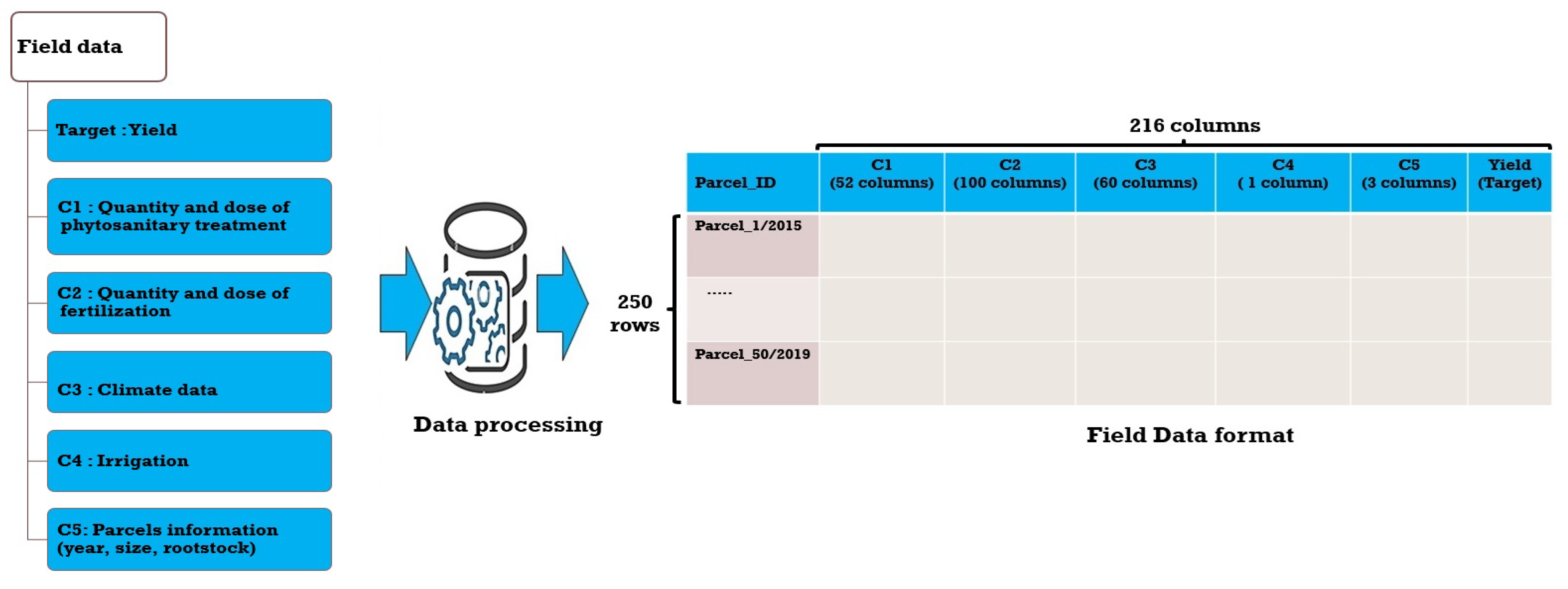
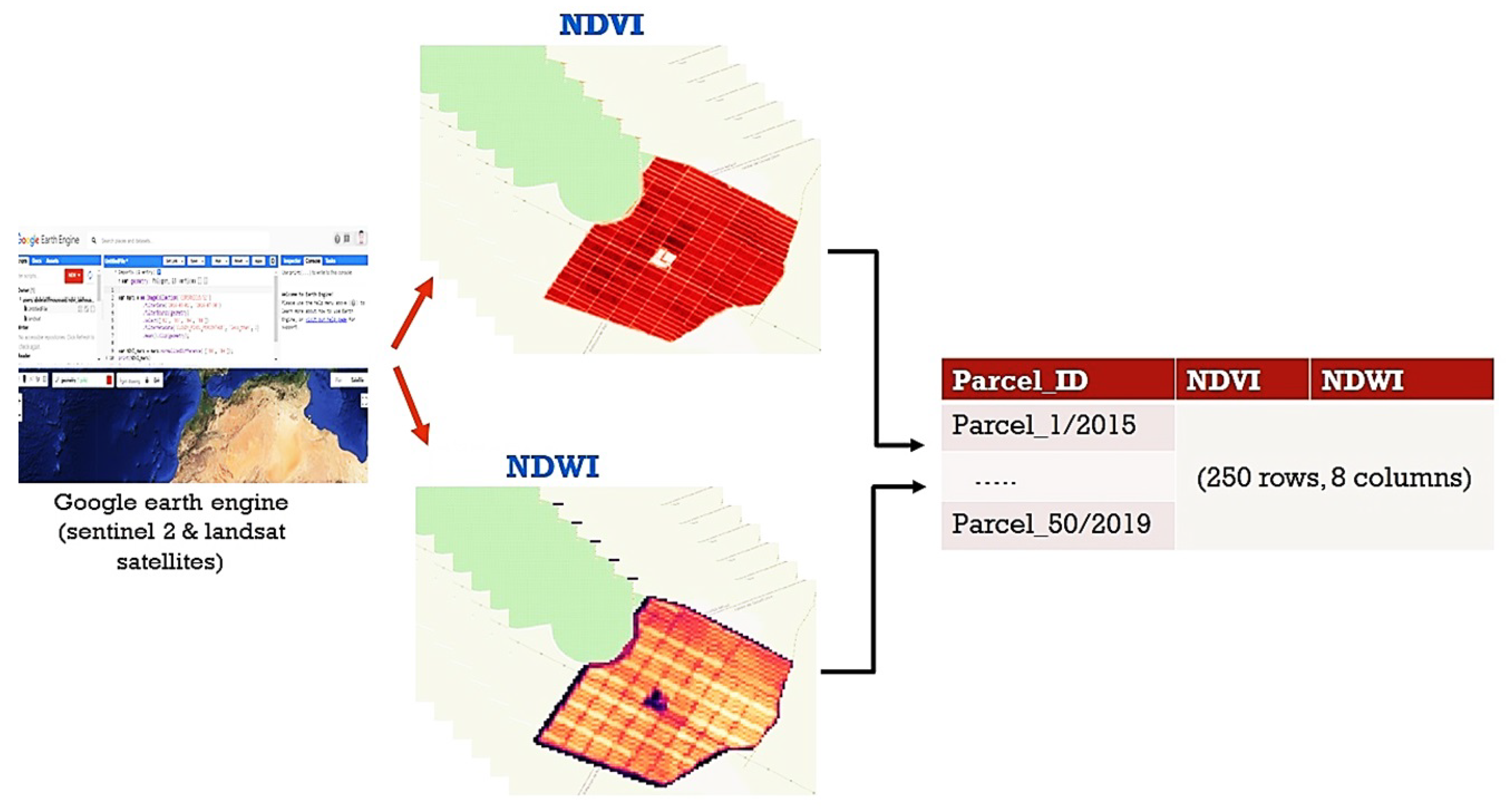
2.2.1. Data Acquisition

Data collection is a vital part of any data science project [30]. In our case, our dataset includes two parts: field data, which is collected directly from the orchard, and spectral data obtained from satellite images. For the first data category, we have 5 years of historical information about irrigation, fertilization, and phytosanitary treatment. Moreover, a climate station is installed inside the orchard to collect daily data on temperature, precipitation, humidity, wind speed, and solar radiation. In detail, our field dataset is made up of 250 rows, which represent 50 parcels multiplied by 5 years; these data present the quantity of water irrigated in each parcel for each agricultural year, the dose of phytosanitary treatment used, and the different products with the doses that were used to fertilize the parcels, as well as the climatic data. This data is labeled according to the yield of each parcel during each crop year.

The different products used for fertilization and phytosanitary treatment during the 5 years of data are presented in the

Table 1. Fertilization and phytosanitary treatment products.

Fertilization products

- N (nitrogen) - P(phosphorus) - K (Potassium) - NITRIC ACID - PHOSPHORIC ACID - SULFURIC ACID -ACTICAL - ACTIRAIL - ENABLE - AMMONITRATE - Aggis TE Fe6 - BERELEX (Lozenge) - BIOCURE -BORONIA POWDER - BUDMAX - CALICO Ca-Mg - CALCIUM - DEVSOL - FENGIB - FERTILOG 20 - FITOSOL - LIME BLOSSOM - FOSFITAL - MANURE - GOËMAR BM 86 E - GREENSTIM - KRISTAFEED 46N - KYLATE -Kelpak - LIQUID MAP -MAXIM - MICROQUEL - MOLYBDATE - NACAR - CALCIUM NITRATE - POTASH NITRATE - NITROPLUS - NITROPLUS 9+B GA - SEQUESTREN - SIAPTON - SOLQUEL - COPPER SULFATE - IRON SULFATE - MANGANESE SULPHATE - SOLUBLE SULPHATE OF POTASH - ZINC SULPHATE - SUPRALEX -Samfer - Stop it - TENSOTEC - UREA - UREA 46% -VIGOMAX

Phytosanitary treatment products

Product against Mites - Product against Whitefly - Product against Ceratitis - Product against Snails - Product against California rental - Product against aphids - growth regulator - Product against Thrips

.

The second part of the data (spectral information) is composed of two elements: the Normalized Difference Vegetation Index (NDVI) and the Normalized Difference Water Stress Index (NDWI). These indices are obtained from the sentinel-2 [31] and Landsat [32] satellite imagery, which are highly used in the agriculture field [33,34,35].

The NDVI and NDWI formulas are presented in Equations (1) and (2), respectively, of which near-infrared radiation (NIR) is a reflection in the near-infrared spectrum, the Red is a reflection in the red range of the spectrum, and the Short Wave Infrared (SWIR) is the part of the range with wavelengths in the range of 0.841–0.876 nm.

$$NDVI=(NIR-Red)/(NIR+Red)$$

(1)

$$NDWI=(NIR-SWIR)/(NIR+SWIR)$$

(2)

2.2.2. Data Processing

To exploit the maximum field data in order to create a robust prediction model, each part of the data (factor) is prepared according to a specific method as follows:

Phytosanitary treatment (C1): It consists of the quantities and doses used over the agricultural year. These products are used against certain specific diseases which attack citrus fruits such as mites, ceratitis, snails, etc. (Table 1). Sometimes, these products are used in certain parcels among all, or in a specific year only. We therefore assigned a 0 to the empty cells to complete our dataset. After having prepared this part of the data, we obtained 52 columns, which contain the quantities and doses used in each parcel during the 5 years.

Fertilization (C2): It consists of the quantities and doses of fertilization products used during each year in each parcel (Table 1). For the preparation method, the same operation used for phytosanitary treatment was followed for the fertilization part; so, we obtained 100 columns including the different quantities and doses of fertilization products used in each parcel during each year.

Climate (C3): It is composed of 5 variables (temperature, precipitation, humidity, wind speed, and solar radiation), which were averaged for each month to obtain 60 columns.

Irrigation (C4): We have just 1 column, which contains the total amount of water used in each parcel during each year.

Parcels information (C5): It consists of some fixed information about each parcel such as the size, the root-stock type, and agricultural year.

Yield (target): It presents the number of crates from each parcel after the harvest period. We normalized it and, of course, this normalization keeps the same distribution and percentage difference.

Finally, we combined all these columns to obtain a large dataset with a size of 216,250 (columns, rows) labeled by the yield of each parcel during the 5 years. Figure 1 summarizes these factors and how we prepared them to construct the field data.

For spectral information, we used Google Earth Engine (cloud) to extract NDVI and NDWI indices over a specific period (8 months) from March to October each year. This decision was made based on the life cycle of the Afourer mandarin in Morocco, which begins in March after the harvest period. Then, we took the average of these indices during the 8 months to obtain the NDVI and NDWI matrices per each parcel during each year. Finally, we extracted the mean, max, min, and mode values from those bands to build our spectral data (Figure 2).

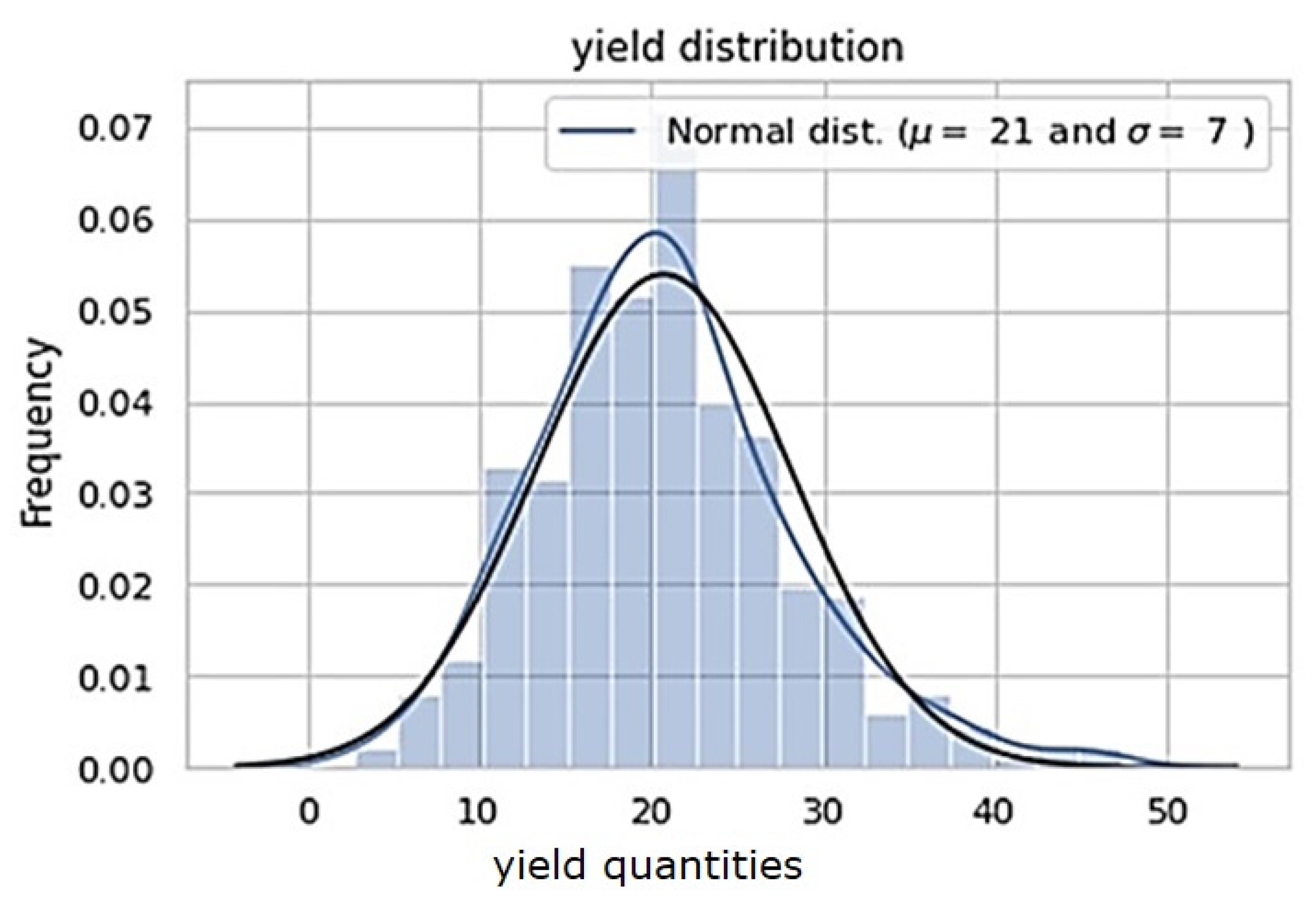
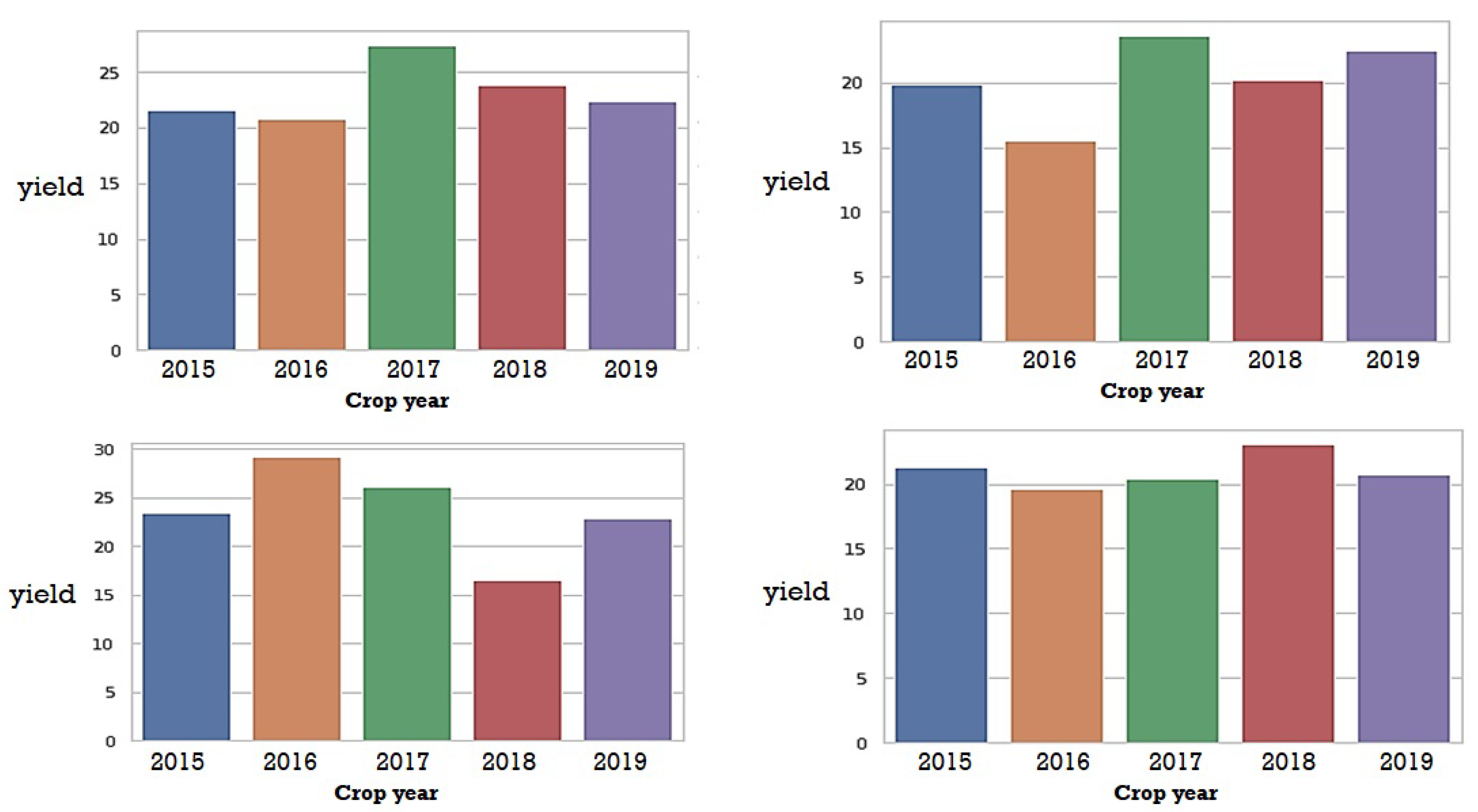
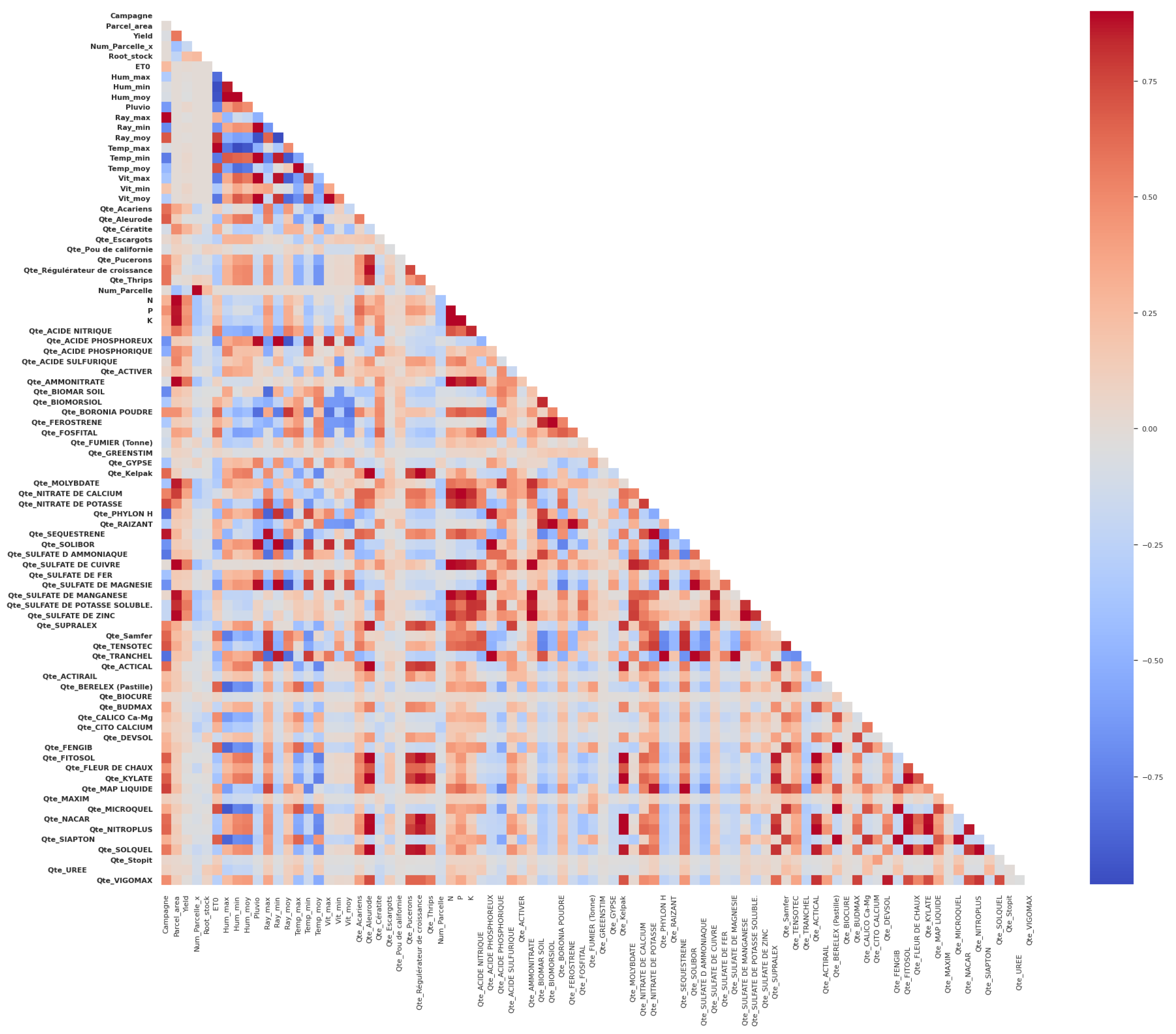
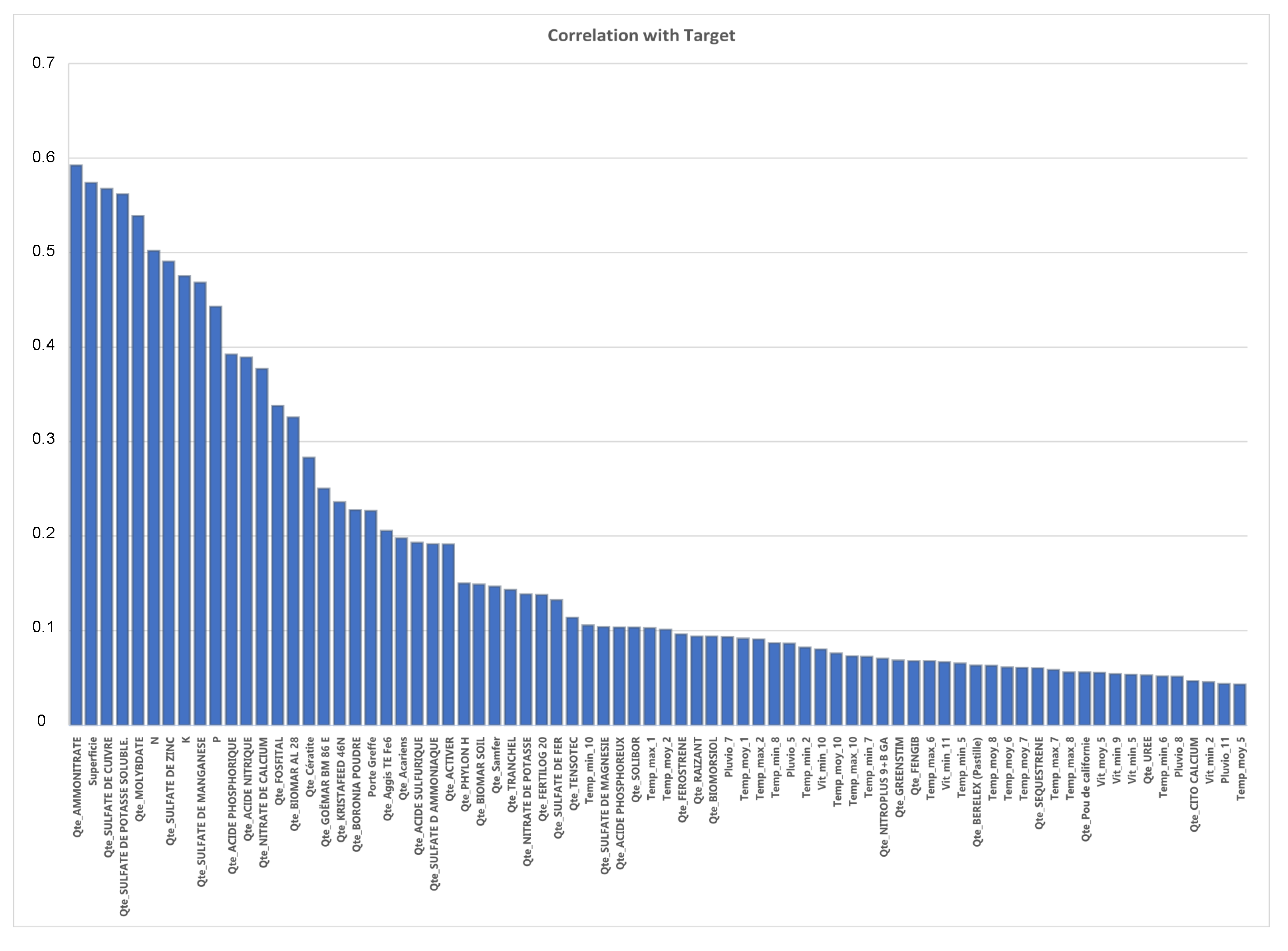
2.2.3. Data Exploration

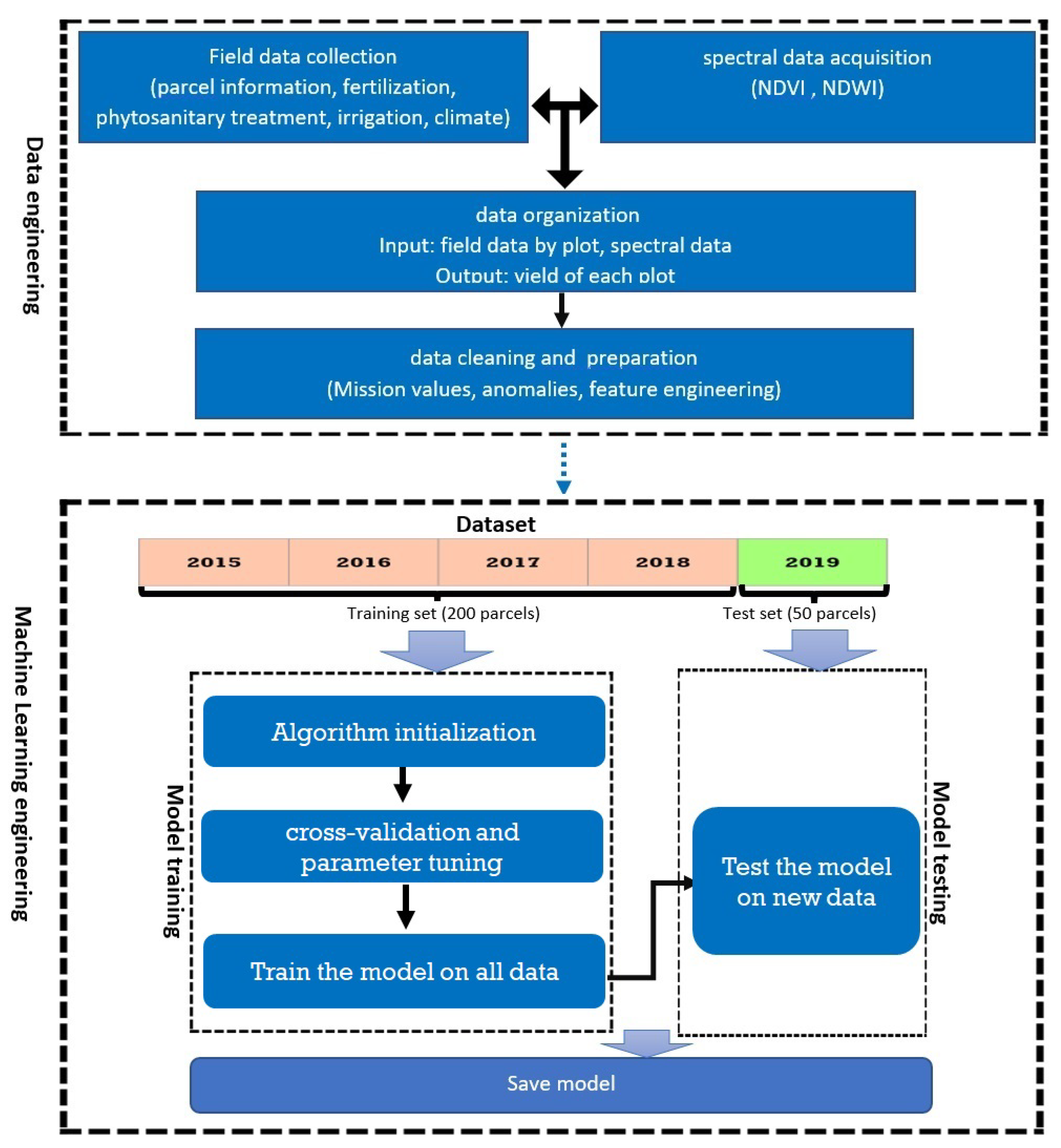
Before starting the prediction phase using machine learning algorithms, data exploration is a vital phase that helps to have a clear view of the variables and make the necessary feature engineering. In our case, the target distribution (Figure 3), which starts from 2015 to 2019 with 50 parcels, follows a normal distribution, which is very beneficial for machine learning models.

In addition, Figure 4 presents the variation of the yield in some parcels during the 5 years of our data. The bar graphs in the figure show four samples taken at random from different locations in the orchard. Additionally, in each graph, the bars presents the normalized yield by year. As you see, we have a considerable variation of yield in each parcel; this means that there are other factors related to field and climate influencing this yield.

In order to summarize the dataset, we tried to create a correlation matrix which represents all the information hidden behind the features, the relationship between them, as well as their relationship with the target [36]. Figure 5 presents a correlation matrix (heatmap) of the input variables. As we have many variables, and it is impossible to visualize them in the figure, we tried to reduce the number of variables; for example, we averaged the values for each climatic variable over each year. Moreover, for fertilization and phytosanitary treatment products, we only visualized their quantity.

As you see in the heatmap, a lot of variables are positively correlated (red color), and others are negatively correlated (blue color), which means that there is a good dependency between them. For example, we see that the climatic data are correlated with phytosanitary treatment features. The interpretation of these results is that there are diseases which attack the trees at a specific time of the year (for example Ceratitis capitata, which attacks citrus fruits in winter [37]). Moreover, the correlation between fertilization and climate is strongly demonstrated for the reason that the quantities of fertilization used during the year sometimes depend on high temperature or on water stress, which is correlated with the temperature [38]. This dependency is very important for the prediction algorithms to perform good training, and it can help us to make some feature engineering.

Regarding the correlation between the input variables and the target (Figure 6), we found that some variables such as quantity AMMONITRATE, parcels size, nitrogen, phosphorus, potassium, etc., have a good correlation of up to 0.5 and 0.6, which is a positive indicator before starting the prediction phase. We also found that the variables related to the phytosanitary treatment have a good correlation with the target, because the quantities and the products used depend on the disease that attacked the parcel, which surely influence the yield of this parcel. Generally, there is an agricultural expert who checks the parcels each time, and when they observe a disease or an alteration requiring a specific product, they initiate the treatment operation in the infected area.

2.3. Our Approach

Machine learning algorithms have demonstrated good performance in recent years, which are used in most fields [39,40]. In our case, after collecting and preparing our dataset, we decided to use machine learning algorithms to predict the yield of citrus fruits, in particular the Afourer variety.

Technically, we have a regression problem, as we are trying to predict yield quantities. Basically, we have a supervised learning problem with regression prediction. In this case, there are linear algorithms such as linear regression, lasso regression, ridge regression, etc. These algorithms analyze the relationships between the dependent variable Y and the set of independent variables X. This relationship is expressed in the form of an equation that predicts the values of the target variable in the form of a linear combination of parameters [41].

Other algorithms are widely used, such as decision tree regression, which determines the best feature in the training dataset after dividing it into subsets containing the possible values of the best feature. After this, the algorithm recursively generates new decision trees using the created data subsets. When there is no more prediction based on this data, the algorithm stops and returns the final model [42].

In addition, an ensembling learning technique has been used in recent years. This technique builds multiple models with different parameters to increase the prediction score. There are two main ensembling methods, boosting (sequential) and bagging (parallel) [43]. In the boosting ensemble learning method, the models train sequentially, and they try to learn until they make mistakes. Regarding the bagging method, the models are trained simultaneously, each one of them trains on a subsample of data, and the final model builds based on voting among the final predictions [44].

Through ensembling learning techniques, several powerful algorithms have been built, such as CatBoost Regressor, Light Gradient Boosting Machine, Random Forest Regressor, Extreme Gradient Boosting, etc. [45,46]. Finally, a cross-validation technique with a tuning parameter algorithm is needed to obtain the hyper-parameters and avoid overfitting [47].

In our case, we split our dataset into two parts, the training part and the test part. In fact, this split is not random, we tried to imagine that our model could be used to predict the yield of an agricultural year before the harvest period, so we took the data for the years 2015, 2016, 2017, and 2018 to train the models, and we made the test using the year 2019 (we used the past to predict the future). Figure 7 summarizes the steps of our approach.

To avoid overfitting and to select the best algorithm, we used the K-fold technique with 4 folds in the training and validation phase. During each round, a grid-search technique is applied to find the best parameters for each algorithm. After the four iterations, we obtained an average score, which can be considered as the trust validation score. Then, we tested the models on another part of the data (test), which is completely new, in order to have the prediction score.

Figure 8 illustrates the cross-validation steps.

3. Results and Discussion

To choose the best algorithm that fits our dataset, we tested several types of algorithms: linear, decision trees, and some ensembling algorithms.

The metrics used for scoring are MAE and MSE, whose formulas are presented successively in Equations (3) and (4), where $y_i$ is the prediction, $x_i$ is the real value, and n is the total number of data points.

$$MAE=\frac{{\sum }_{i=1}^n|x_i-y_i\left|\right)}{n}$$

(3)

$$MSE=\frac{{\sum }_{i=1}^n{(x_i-y_i)}^2}{n}$$

(4)

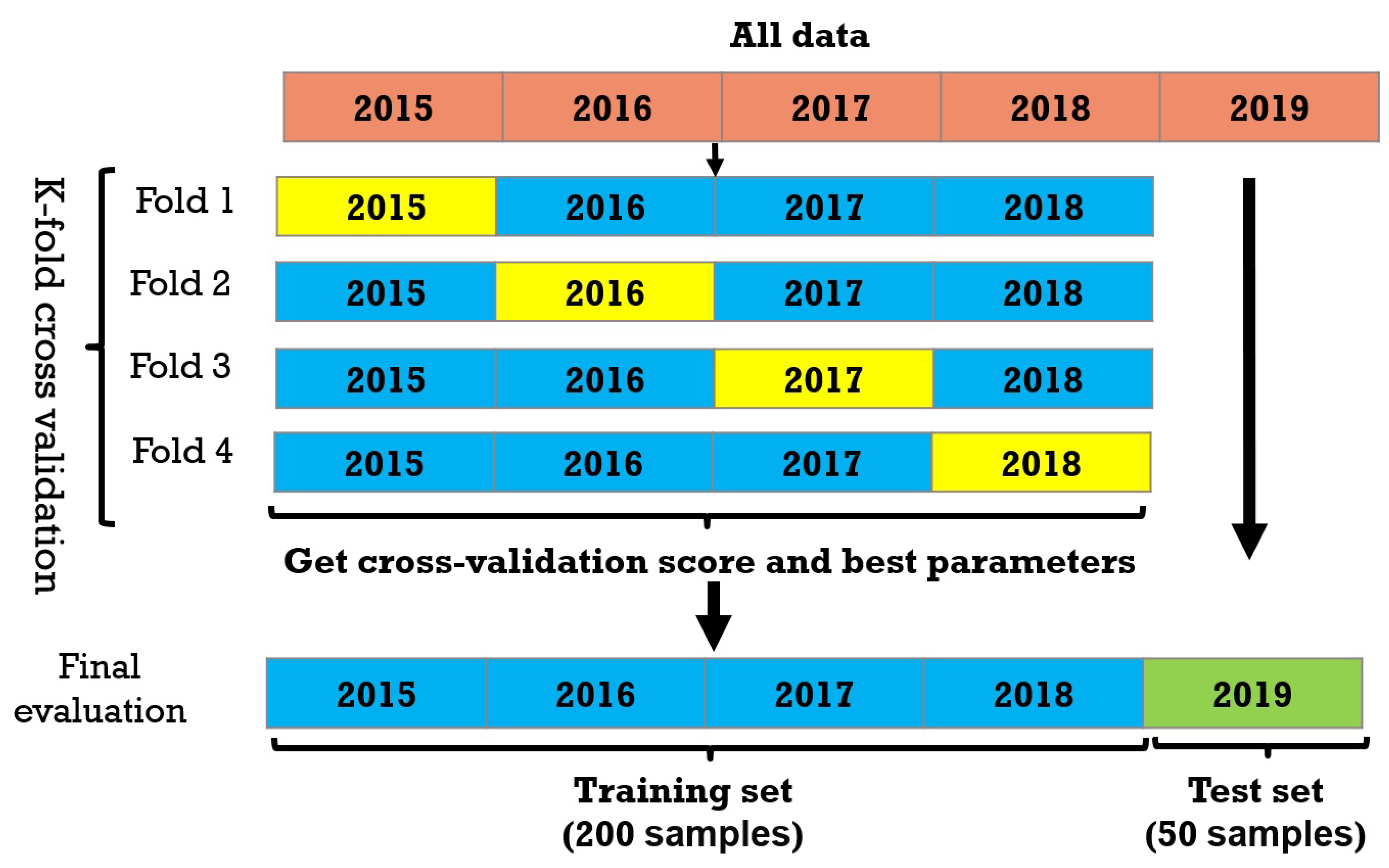
3.1. Cross-Validation and Model Selection

In the first time, we used all the data (field and spectral data) to perform cross-validation. A k-fold technique with k = 4 is used, and the scores obtained are presented in

Table 2. Cross-validation scores including MAE and MSE metrics.

	Model	MAE	MSE
ridge	Ridge Regression	0.3225	0.1676
catboost	CatBoost Regressor	0.2631	0.1174
gbr	Gradient Boosting Regressor	0.2608	0.1107
rf	Random Forest Regressor	0.2677	0.1175
en	Elastic Net	0.2963	0.1435
ada	AdaBoost Regressor	0.2618	0.1158
br	Bayesian Ridge	0.2932	0.1392
lasso	Lasso Regression	0.2918	0.1380
et	Extra Trees Regressor	0.2767	0.1303
lightgbm	Light Gradient Boosting Machine	0.2829	0.1311
xgboost	Extreme Gradient Boosting	0.3192	0.1586
huber	Huber Regressor	0.3506	0.2661
omp	Orthogonal Matching Pursuit	0.2585	0.1092
llar	Lasso Least Angle Regression	0.3025	0.1667
dt	Decision Tree Regressor	0.3468	0.2114
knn	K Neighbors Regressor	0.2705	0.1204
lr	Linear Regression	0.6027	0.6159

.

The results in Table 2 show a good performance in the prediction, with an average score approaching 0.11 (MSE), this indicates that the data really helped the models to train well. Moreover, the Orthogonal Matching Pursuit algorithm [48] gave a good score of 0.10 (MSE CV).

After performing cross-validation and parameter tuning using the grid-search algorithm, we tried to train the new models on the all the training datasets and test them on other new data that they have not really seen before (data corresponding to the year 2019). Moreover, to see the importance of field data and the added value of spectral data, we tested the models on two parts of data, the first part corresponds to the indicators collected in the field (field data), and the second part contains the total data which contain the spectral indicators (field data + spectral information). The test results are presented in

Table 3. Yield prediction results including MAE and MSE metrics.

Model		Field Dat		Field + Spectral Data
		MAE	MSE	MAE	MSE
ridge	Ridge Regression	0.2680	0.1140	0.2525	0.1034
catboost	CatBoost Regressor	0.2477	0.1057	0.2477	0.1057
gbr	Gradient Boosting Regressor	0.2649	0.1281	0.2475	0.1024
rf	Random Forest Regressor	0.2689	0.1287	0.2497	0.1046
en	Elastic Net	0.2760	0.1287	0.2536	0.1049
ada	AdaBoost Regressor	0.2682	0.1333	0.2484	0.1085
br	Bayesian Ridge	0.2758	0.1299	0.2585	0.1093
lasso	Lasso Regression	0.2759	0.1265	0.2592	0.1099
et	Extra Trees Regressor	0.2594	0.1187	0.2452	0.1092
lightgbm	Light Gradient Boosting Machine	0.2593	0.1153	0.2610	0.1138
xgboost	Extreme Gradient Boosting	0.2926	0.1703	0.2645	0.1165
huber	Huber Regressor	0.3816	0.2752	0.2825	0.1305
omp	Orthogonal Matching Pursuit	0.2489	0.0843	0.2315	0.0748
llar	Lasso Least Angle Regression	0.3036	0.1666	0.2982	0.1665
dt	Decision Tree Regressor	0.3187	0.1828	0.3270	0.1678
knn	K Neighbors Regressor	0.3166	0.1789	0.3327	0.2036
lr	Linear Regression	0.5705	0.5696	0.4129	0.3327

.

As you see in Table 3, the scores obtained by the chosen algorithms are very close to each other, but the OMP algorithm gave good prediction scores, which are (0.2489 (MAE) and 0.0843 (MSE)). After adding the NDVI and NDWI indices, the scores improved to (0.2315 (MAE) and 0.0748 (MSE)), which demonstrates the importance of satellite imagery in predicting yield.

The hyper-parameters of the OMP algorithm that we obtained after the grid search, and which were used to train the final model, are: $OrthogonalMatchingPursuit(fit\_intercept=True,n\_nonzero\_coefs=44,normalize=True,precompute=‘auto’,tol=None)$ where the fit_intercept concerning the include an intercept of the model (Boolean), n_nonzero_coefsint, is the desired number of non-zero entries in the solution. The normalized parameter, which concerns the normalization of input data or not, precomputes to speed up the calculations, and tol is the maximum norm of the residual.

To find out more about the OMP algorithm, the Algorithm 1 contains its learning steps and how it chooses the right variables.

The key idea of the OMP algorithm is that it tries to reconstruct the support set A of x iteratively, starting with $A=$. Then, in each iteration l, the inner products between the columns of $\varphi$ and the residuals $r^{l-1}$ are calculated, then the absolute value of this inner product is added to A. Here, the residual $r^{l-1}$ from the former iteration represents the component of the measurement vector y that cannot be spanned by the columns of $\varphi$ indexed by A. In this way, the columns $\varphi$, which are the most relative to y, are iteratively chosen [48].

In general, the OMP algorithm classifies the variables by their correlation with the target before integrating them one by one for learning [49]. This technique is very effective when the dataset contains many variables with a minimum of rows (small dataset).

Algorithm 1 Orthogonal Matching Pursuit

Input: $y,\varphi$ Initialization: $r^0=y,A^0=,l=0;$ Repeat      $l=l+1$;      match step:      $h^l={\Phi }^T{r}^{l-1}$;      identify step:      $A^l=A^{L-1}\cup \left\{argma{x}_j\left|h^l\left(j\right)\right|\right\}$;      update step:      $x^{l}argmi{n}_{z:supp\left(z\right)\subseteq A^l}{\Vert y-\varphi z\Vert }_2$;      $r^l=y-\varphi x^l$; Until stop criterion satisfied; output: $x^k$;

3.2. Discussion of Results

In order to better understand and discuss the results obtained, we calculated the percentage error between the measured value and the actual value for each parcel (Formula (5)).

$$\mathrm{percentage}\mathrm{error}=\frac{|\mathrm{Measured}\mathrm{value}-\mathrm{True}\mathrm{value}|}{\mathrm{True}\mathrm{value}}$$

(5)

Table 4. Yield prediction percentage error per parcel.

	Field Data			Field + Spectral Data
Parcel_ID	Parcel Information and Climate	Parcel Information, Climate and Phytosanitary Treatment	Parcel Information, Climate, Phytosanitary Treatment and Fertilization	Parcel Information, Climate, Phytosanitary Treatment Fertilization and Spectral Data
0	0.3789	0.2853	0.2738	0.2731
1	0.2309	0.1667	0.1564	0.0929
2	0.1739	0.1697	0.1477	0.1424
3	0.3097	0.2397	0.0847	0.0421
4	0.5509	0.4903	0.23	0.1822
5	0.3201	0.2697	0.2642	0.2174
6	0.7632	0.2803	0.2366	0.1774
7	1.259	0.531	0.3538	0.2465
8	0.8286	0.373	0.2851	0.2353
9	0.8662	0.6127	0.3483	0.2976
10	0.6043	0.3091	0.1267	0.0846
11	0.2791	0.2722	0.2698	0.2319
12	0.2436	0.2252	0.1425	0.0966
13	0.2943	0.0306	0.1619	0.1175
14	0.4927	0.2881	0.2317	0.1954
15	0.3473	0.2983	0.1745	0.1516
16	0.2703	0.2523	0.2121	0.1651
17	0.2965	0.2625	0.2411	0.193
18	0.3455	0.2803	0.0972	0.0937
19	0.3957	0.3198	0.2981	0.2291
20	0.4877	0.396	0.1861	0.1401
21	0.7791	0.1548	0.0373	0.0191
22	0.3168	0.2838	0.2621	0.2523
23	0.3878	0.3806	0.3188	0.2805
24	0.3236	0.2997	0.2981	0.2918
25	0.1691	0.1638	0.1683	0.1625
26	0.3772	0.2373	0.0867	0.0489
27	0.3646	0.3188	0.0777	0.0701
28	0.2822	0.2492	0.1351	0.1484
29	0.44	0.3521	0.328	0.2698
30	0.0893	0.0589	0.0229	0.0155
31	0.2962	0.2553	0.0319	0.0037
32	0.3527	0.3522	0.2478	0.2183
33	0.2291	0.2221	0.2203	0.196
34	1.5524	0.3627	0.2954	0.0204
35	0.2556	0.2474	0.2297	0.2169
36	0.7512	0.5378	0.2104	0.1904
37	0.3316	0.3034	0.1884	0.1302
38	0.2945	0.294	0.2239	0.1986
39	0.4909	0.3789	0.1237	0.1027
40	0.6537	0.4716	0.2405	0.2244
41	0.1862	0.1775	0.1761	0.1563
42	0.4248	0.3129	0.279	0.2025
43	0.9766	0.8478	0.3093	0.2596
44	0.2824	0.0474	0.0357	0.0353
45	0.3354	0.318	0.3145	0.2666
46	0.208	0.1935	0.1888	0.1326
47	0.3784	0.3301	0.247	0.1955
48	0.3636	0.3032	0.1225	0.0637
49	0.3317	0.2708	0.219	0.168
Average	0.4392	0.3015	0.2032	0.1629

contains the prediction scores obtained by our model on 50 test parcels. The first column shows the scores obtained using parcel information and climate data only, the second column presents the scores after adding phytosanitary treatment data, the third column shows the scores after adding fertilization data, and finally, the last column contains the scores that are obtained using all field data combined with spectral information (NDVI and NDWI).

As you see in Table 4, the parcel information combined with climate data (column 1) does not give a good yield prediction result, the average prediction does not exceed 0.43, and some parcels have scores ranging from up to 100% error. In general, the climatic data are presented globally and are identical for all the parcels, this does not really help the model to exploit the data, because it finds the same input with different output (yields), hence the fact that parcel information gave meaning to the climate data. After adding the phytosanitary treatment data, the scores are improved to 0.30 on average (column 2). We can clearly see that some parcels have experienced a significant improvement (0,1,3,6,7,8,10,13,21,34 …); this reflects that the yield of these parcels is very correlated with phytosanitary treatments products. Moreover, we can conclude that these parcels are more likely to be exposed to the diseases and insects that affect the crop the most. Other parcels’ prediction scores did not have much difference (2,12,16,23,25,30…), which means that these parcels are little affected, or they are more resistant to diseases than others.

In the third step (column 3), we added the fertilization data. We can clearly see that the average score improved to 0.20; this score is very interesting and clearly shows that the combination of climatic, phytosanitary treatment, and fertilization data is very important for yield prediction. In this sense, we found that the score of the most parcels improved positively. We also see that some parcels, which were not improved before, improved after adding the fertilization data, such as parcel 26, which is predicted with a score of 0.08, and parcel 27 with a score of 0.07. Although some parcels failed to improve their prediction scores, such as the parcels 24 and 45, the prediction results using only field data are quite interesting and original.

Finally, after adding the NDVI and NDWI data, the average error rate went from 0.20 to 0.16, which means that the results improved by more than 4%. Thus, the spectral data played an important role in improving the results of many parcels, such as parcel 1, which went from 15% error to 9%, and parcel 12 from 14% to 9%.

In general, some parcels were predicted with a very good score not exceeding 5% error, such as parcels 3, 21, 26, 30, 31, 34, and 44. Moreover, most of the scores do not exceed 20% error, which indicates that the data used is very interesting, and the approach followed in this study showed the ability to generate excellent predictive results.

To conclude, the results obtained in this study are very satisfactory compared with the state of the art (an average error of no more than 0.162). We tried to work with data (irrigation, fertilization, phytosanitary treatments, and climate) easily collectible thanks to the current evolution of agriculture, and we used open-source satellites that provide free images. Therefore, this solution is inexpensive and farmers can use it to obtain a real idea of the yield before the harvest period.

Finally, a bar chart graph was constructed (Figure 9) to show a visual comparison between actual yield quantities (red color) and the predicted ones (green color). As you see, there are some parcels that are very well-predicted (1,3,26,27,30,31,34,44). Other parcels are very close, and others are not bad (0,11,23,24). However, overall, we are satisfied with these results, and we recommend farmers start collecting field data to obtain a proactive view of their yield.

4. Conclusions

Predicting tree yield is one of the most difficult tasks in modern agriculture. Most of the existing work attempts to predict the productivity of trees by counting their fruits [18,50,51,52]. This method is expensive and difficult, especially in the case of large orchards. In addition, farmers need to know their yield at least one month before harvest and in a simple and fast way. The main contribution of our research is to show the importance of field data in predicting the yield of a parcel of trees.

The results obtained are very good and the power of field data was demonstrated. In particular, data such as fertilization and phytosanitary treatment have greatly helped our prediction model. Moreover, the proposed approach requires only data, it is inexpensive, fast, and generates the result immediately.

Finally, even with the good results obtained, our team continues daily data collection, and we are sure that feeding our dataset will improve the prediction scores. Moreover, we trust that this experience can be generalized to other tree crops.

References

1. Patrício, D.I.; Rieder, R. Computer vision and artificial intelligence in precision agriculture for grain crops: A systematic review. Comput. Electron. Agric. 2018, 153, 69–81. [Google Scholar] [CrossRef] [Green Version]
2. Linaza, M.T.; Posada, J.; Bund, J.; Eisert, P.; Quartulli, M.; Döllner, J.; Pagani, A.; G Olaizola, I.; Barriguinha, A.; Moysiadis, T.; et al. Data-driven artificial intelligence applications for sustainable precision agriculture. Agronomy 2021, 11, 1227. [Google Scholar] [CrossRef]
3. Sharma, A.; Jain, A.; Gupta, P.; Chowdary, V. Machine learning applications for precision agriculture: A comprehensive review. IEEE Access 2020, 9, 4843–4873. [Google Scholar] [CrossRef]
4. Lu, Y.; Young, S. A survey of public datasets for computer vision tasks in precision agriculture. Comput. Electron. Agric. 2020, 178, 105760. [Google Scholar] [CrossRef]
5. Rashid, M.; Bari, B.S.; Yusup, Y.; Kamaruddin, M.A.; Khan, N. A comprehensive review of crop yield prediction using machine learning approaches with special emphasis on palm oil yield prediction. IEEE Access 2021, 9, 63406–63439. [Google Scholar] [CrossRef]
6. Michler, J.D.; Tjernström, E.; Verkaart, S.; Mausch, K. Money matters: The role of yields and profits in agricultural technology adoption. Am. J. Agric. Econ. 2019, 101, 710–731. [Google Scholar] [CrossRef] [Green Version]
7. Anderson, N.T.; Walsh, K.B.; Wulfsohn, D. Technologies for forecasting tree fruit load and harvest timing—From ground, sky and time. Agronomy 2021, 11, 1409. [Google Scholar] [CrossRef]
8. Yan, B.; Fan, P.; Lei, X.; Liu, Z.; Yang, F. A real-time apple targets detection method for picking robot based on improved YOLOv5. Remote Sens. 2021, 13, 1619. [Google Scholar] [CrossRef]
9. Parico, A.I.B.; Ahamed, T. Real time pear fruit detection and counting using YOLOv4 models and deep SORT. Sensors 2021, 21, 4803. [Google Scholar] [CrossRef]
10. Wan, S.; Goudos, S. Faster R-CNN for multi-class fruit detection using a robotic vision system. Comput. Netw. 2020, 168, 107036. [Google Scholar] [CrossRef]
11. Nawaz, R.; Abbasi, N.A.; Hafiz, I.A.; Khalid, A. Impact of climate variables on growth and development of Kinnow fruit (Citrus nobilis Lour x Citrus deliciosa Tenora) grown at different ecological zones under climate change scenario. Sci. Hortic. 2020, 260, 108868. [Google Scholar] [CrossRef]
12. Wan, L.J.; Tian, Y.; He, M.; Zheng, Y.Q.; Lyu, Q.; Xie, R.J.; Ma, Y.Y.; Deng, L.; Yi, S.L. Effects of Chemical Fertilizer Combined with Organic Fertilizer Application on Soil Properties, Citrus Growth Physiology, and Yield. Agriculture 2021, 11, 1207. [Google Scholar] [CrossRef]
13. Dutta, S.K.; Gurung, G.; Yadav, A.; Laha, R.; Mishra, V.K. Factors associated with citrus fruit abscission and management strategies developed so far: A review. N. Z. J. Crop Hortic. Sci. 2022, 1–22. [Google Scholar] [CrossRef]
14. Vincent, C.; Morillon, R.; Arbona, V.; Gómez-Cadenas, A. Citrus in changing environments. In The Genus Citrus; Elsevier: Amsterdam, The Netherlands, 2020; pp. 271–289. [Google Scholar]
15. Moussaid, A.; El Fkihi, S.; Zennayi, Y. Citrus Orchards Monitoring based on Remote Sensing and Artificial Intelligence Techniques: A Review of the Literature. In Proceedings of the 2nd International Conference on Advanced Technologies for Humanity—ICATH, Rabat, Morocco, 20–21 November 2020; IEEE: New York, NY, USA, 2020; pp. 172–178. [Google Scholar]
16. Mngadi, M.; Odindi, J.; Mutanga, O. The utility of Sentinel-2 spectral data in quantifying above-ground carbon stock in an urban reforested landscape. Remote Sens. 2021, 13, 4281. [Google Scholar] [CrossRef]
17. Galphade, M.; More, N.; Wagh, A.; Nikam, V. Crop Yield Prediction Using Weather Data and NDVI Time Series Data. In Advances in Data Computing, Communication and Security; Springer: Berlin/Heidelberg, Germany, 2022; pp. 261–271. [Google Scholar]
18. Moussaid, A.; Fkihi, S.E.; Zennayi, Y. Tree Crowns Segmentation and Classification in Overlapping Orchards Based on Satellite Images and Unsupervised Learning Algorithms. J. Imaging 2021, 7, 241. [Google Scholar] [CrossRef]
19. Ye, X.; Sakai, K.; Manago, M.; Asada, S.i.; Sasao, A. Prediction of citrus yield from airborne hyperspectral imagery. Precis. Agric. 2007, 8, 111–125. [Google Scholar] [CrossRef]
20. De Ollas, C.; Morillón, R.; Fotopoulos, V.; Puértolas, J.; Ollitrault, P.; Gómez-Cadenas, A.; Arbona, V. Facing climate change: Biotechnology of iconic Mediterranean woody crops. Front. Plant Sci. 2019, 10, 427. [Google Scholar] [CrossRef]
21. Vogel, E.; Donat, M.G.; Alexander, L.V.; Meinshausen, M.; Ray, D.K.; Karoly, D.; Meinshausen, N.; Frieler, K. The effects of climate extremes on global agricultural yields. Environ. Res. Lett. 2019, 14, 054010. [Google Scholar] [CrossRef]
22. Nagaz, K.; El Mokh, F.; Ben Hassen, N.; Masmoudi, M.; Ben Mechlia, N.; Baba Sy, M.; Belkheiri, O.; Ghiglieri, G. Impact of deficit irrigation on yield and fruit quality of orange Trees (Citrus sinensis, l. Osbeck, cv. Meski maltaise) in southern Tunisia. Irrig. Drain. 2020, 69, 186–193. [Google Scholar] [CrossRef] [Green Version]
23. Cai, A.; Xu, M.; Wang, B.; Zhang, W.; Liang, G.; Hou, E.; Luo, Y. Manure acts as a better fertilizer for increasing crop yields than synthetic fertilizer does by improving soil fertility. Soil Tillage Res. 2019, 189, 168–175. [Google Scholar] [CrossRef]
24. Morugán-Coronado, A.; Linares, C.; Gómez-López, M.D.; Faz, Á.; Zornoza, R. The impact of intercropping, tillage and fertilizer type on soil and crop yield in fruit orchards under Mediterranean conditions: A meta-analysis of field studies. Agric. Syst. 2020, 178, 102736. [Google Scholar] [CrossRef]
25. Buczko, U.; van Laak, M.; Eichler-Löbermann, B.; Gans, W.; Merbach, I.; Panten, K.; Peiter, E.; Reitz, T.; Spiegel, H.; von Tucher, S. Re-evaluation of the yield response to phosphorus fertilization based on meta-analyses of long-term field experiments. Ambio 2018, 47, 50–61. [Google Scholar] [CrossRef] [PubMed] [Green Version]
26. Li, Z.; Zhang, R.; Xia, S.; Wang, L.; Liu, C.; Zhang, R.; Fan, Z.; Chen, F.; Liu, Y. Interactions between N, P and K fertilizers affect the environment and the yield and quality of satsumas. Glob. Ecol. Conserv. 2019, 19, e00663. [Google Scholar] [CrossRef]
27. Coble, K.H.; Mishra, A.K.; Ferrell, S.; Griffin, T. Big data in agriculture: A challenge for the future. Appl. Econ. Perspect. Policy 2018, 40, 79–96. [Google Scholar] [CrossRef] [Green Version]
28. Cravero, A.; Sepúlveda, S. Use and adaptations of machine learning in big data—Applications in real cases in agriculture. Electronics 2021, 10, 552. [Google Scholar] [CrossRef]
29. Ihbach, F.Z.; Kchikach, A.; Jaffal, M.; El Azzab, D.; Chalikakis, K.; Mazzili, N.; Guerin, R.; Jourani, E.S. Study of an Aquifer in a Semi-arid Area Using MRS, FDEM, TDEM and ERT Methods (Youssoufia and Khouribga, Morocco). In Proceedings of the Conference of the Arabian Journal of Geosciences, Hammamet, Tunisia, 12–15 November 2018; Springer: Berlin/Heidelberg, Germany, 2018; pp. 73–76. [Google Scholar]
30. Roh, Y.; Heo, G.; Whang, S.E. A survey on data collection for machine learning: A big data-ai integration perspective. IEEE Trans. Knowl. Data Eng. 2019, 33, 1328–1347. [Google Scholar] [CrossRef] [Green Version]
31. Segarra, J.; Buchaillot, M.L.; Araus, J.L.; Kefauver, S.C. Remote sensing for precision agriculture: Sentinel-2 improved features and applications. Agronomy 2020, 10, 641. [Google Scholar] [CrossRef]
32. Leslie, C.R.; Servina, L.O.; Miller, H.M. Landsat and Agriculture: Case Studies on the Uses and Benefits of Landsat Imagery in Agricultural Monitoring and Production; US Department of the Interior, US Geological Survey: Reston, VA, USA, 2017.
33. Shanmugapriya, P.; Rathika, S.; Ramesh, T.; Janaki, P. Applications of remote sensing in agriculture-A Review. Int. J. Curr. Microbiol. Appl. Sci. 2019, 8, 2270–2283. [Google Scholar] [CrossRef]
34. Giovos, R.; Tassopoulos, D.; Kalivas, D.; Lougkos, N.; Priovolou, A. Remote sensing vegetation indices in viticulture: A critical review. Agriculture 2021, 11, 457. [Google Scholar] [CrossRef]
35. Sishodia, R.P.; Ray, R.L.; Singh, S.K. Applications of remote sensing in precision agriculture: A review. Remote Sens. 2020, 12, 3136. [Google Scholar] [CrossRef]
36. Rickman, J.; Balasubramanian, G.; Marvel, C.; Chan, H.; Burton, M.T. Machine learning strategies for high-entropy alloys. J. Appl. Phys. 2020, 128, 221101. [Google Scholar] [CrossRef]
37. Khfif, K.; Mokrini, F.; Sbaghi, M. Population monitoring of males steriles of Mediterranean fruit fly (Ceratitis capitata Wiedemann, 1824) in citrus orchards of the Moulouya region. Afr. Mediterr. Agric. J. 2022, 135, 123–135. [Google Scholar]
38. Otero, A.; Goni, C.; Jifon, J.; Syvertsen, J. High temperature effects on citrus orange leaf gas exchange, flowering, fruit quality and yield. In Proceedings of the IX International Symposium on Integrating Canopy, Rootstock and Environmental Physiology in Orchard Systems 903, Geneva, NY, USA, 4–8 August 2008; pp. 1069–1075. [Google Scholar]
39. Emmert-Streib, F.; Yli-Harja, O.; Dehmer, M. Explainable artificial intelligence and machine learning: A reality rooted perspective. Wiley Interdiscip. Rev. Data Min. Knowl. Discov. 2020, 10, e1368. [Google Scholar] [CrossRef]
40. Linardatos, P.; Papastefanopoulos, V.; Kotsiantis, S. Explainable AI: A review of machine learning interpretability methods. Entropy 2020, 23, 18. [Google Scholar] [CrossRef] [PubMed]
41. Wang, P.; Mou, S.; Lian, J.; Ren, W. Solving a system of linear equations: From centralized to distributed algorithms. Annu. Rev. Control. 2019, 47, 306–322. [Google Scholar] [CrossRef]
42. Jiao, S.; Song, J.; Liu, B. A Review of Decision Tree Classification Algorithms for Continuous Variables. In Proceedings of the Journal of Physics: Conference Series, The 2020 second International Conference on Artificial Intelligence Technologies and Application (ICAITA), Dalian, China, 21–23 August 2020; Volume 1651, p. 012083. [Google Scholar]
43. Huettmann, F. Boosting, Bagging and Ensembles in the Real World: An Overview, some Explanations and a Practical Synthesis for Holistic Global Wildlife Conservation Applications Based on Machine Learning with Decision Trees. In Machine Learning for Ecology and Sustainable Natural Resource Management; Springer: Berlin/Heidelberg, Germany, 2018; pp. 63–83. [Google Scholar]
44. Azmi, S.S.; Baliga, S. An Overview of Boosting Decision Tree Algorithms utilizing AdaBoost and XGBoost Boosting strategies. Int. Res. J. Eng. Technol. 2020, 7, 6867–6870. [Google Scholar]
45. Hancock, J.T.; Khoshgoftaar, T.M. CatBoost for big data: An interdisciplinary review. J. Big Data 2020, 7, 1–45. [Google Scholar] [CrossRef]
46. Kadiyala, A.; Kumar, A. Applications of python to evaluate the performance of decision tree-based boosting algorithms. Environ. Prog. Sustain. Energy 2018, 37, 618–623. [Google Scholar] [CrossRef]
47. Siedhoff, N.E.; Schwaneberg, U.; Davari, M.D. Machine learning-assisted enzyme engineering. Methods Enzymol. 2020, 643, 281–315. [Google Scholar]
48. Ding, J.; Chen, L.; Gu, Y. Perturbation analysis of orthogonal matching pursuit. IEEE Trans. Signal Process. 2013, 61, 398–410. [Google Scholar] [CrossRef] [Green Version]
49. Khosravy, M.; Gupta, N.; Patel, N.; Duque, C.A. Recovery in compressive sensing: A review. Compressive Sens. Healthc. 2020, 25–42. [Google Scholar] [CrossRef]
50. Koc-San, D.; Selim, S.; Aslan, N.; San, B.T. Automatic citrus tree extraction from UAV images and digital surface models using circular Hough transform. Comput. Electron. Agric. 2018, 150, 289–301. [Google Scholar] [CrossRef]
51. Csillik, O.; Cherbini, J.; Johnson, R.; Lyons, A.; Kelly, M. Identification of citrus trees from unmanned aerial vehicle imagery using convolutional neural networks. Drones 2018, 2, 39. [Google Scholar] [CrossRef]
52. Osco, L.P.; De Arruda, M.d.S.; Junior, J.M.; Da Silva, N.B.; Ramos, A.P.M.; Moryia, É.A.S.; Imai, N.N.; Pereira, D.R.; Creste, J.E.; Matsubara, E.T.; et al. A convolutional neural network approach for counting and geolocating citrus-trees in UAV multispectral imagery. Isprs J. Photogramm. Remote Sens. 2020, 160, 97–106. [Google Scholar] [CrossRef]
Figure 1. Field data preparation.
Informatics 09 00080 g001
Figure 2. Spectral data acquisition.
Informatics 09 00080 g002
Figure 3. Distribution of the target.
Informatics 09 00080 g003
Figure 4. Distribution of yield over the five years of study (a sample of four parcels).
Informatics 09 00080 g004
Figure 5. Correlation matrix between input variables.
Informatics 09 00080 g005
Figure 6. Correlation between input variables and target.
Informatics 09 00080 g006
Figure 7. The overall approach: the approach includes data engineering and machine learning steps.
Informatics 09 00080 g007
Figure 8. Cross-validation and parameters tuning.
Informatics 09 00080 g008
Figure 9. Validation of the results.
Informatics 09 00080 g009