Abstract
Aquatic products are popular among consumers, and their visual quality used to be detected manually for freshness assessment. This paper presents a solution to inspect tuna and salmon meat from digital images. The solution proposes hardware and a protocol for preprocessing images and extracting parameters from the RGB, HSV, HSI, and L*a*b* spaces of the collected images to generate the datasets. Experiments are performed using machine learning classification methods. We evaluated the AutoML models to classify the freshness levels of tuna and salmon samples through the metrics of: accuracy, receiver operating characteristic curve, precision, recall, f1-score, and confusion matrix (CM). The ensembles generated by AutoML, for both tuna and salmon, reached 100% in all metrics, noting that the method of inspection of fish freshness from image collection, through preprocessing and extraction/fitting of features showed exceptional results when datasets were subjected to the machine learning models. We emphasize how easy it is to use the proposed solution in different contexts. Computer vision and machine learning, as a nondestructive method, were viable for external quality detection of tuna and salmon meat products through its efficiency, objectiveness, consistency, and reliability due to the experiments’ high accuracy.
1. Introduction
Aquatic products have received great popularity because of their high nutritional value and delicious taste. When consumed, their quality determines their value and price [1]. This study’s motivation focuses on food security, particularly in consuming fish-based products, ensuring an impartial classification of tuna and salmon meat’s freshness level.
The aquaculture industry has been demanding inspection of fish quality for a long time, since fishery product deterioration happens very quickly through biochemical processes and microbial degradation mechanisms [2]. The examination of foodstuffs for various quality factors is very repetitive, and is also very subjective. Traditionally, visual quality detection is predominantly done by trained specialists, who approach quality assessment in two ways: seeing and feeling. Due to the strong relationship between fish’s freshness and quality, color and odor are widely used to measure freshness levels. Manual processing and grading are inevitably influenced by human factors, such as mistakes, occasional omission in processing, and fatigue. In addition to being costly, this method is highly variable, and decisions are not always consistent between specialists or from day to day [1].
The destruction of fish and the high inspection cost through sensory methods inhibit the scalability of these quality characteristics. The increased industrial production of tuna and salmon makes the quick and accurate assessment of the fish’s freshness a significant challenge [3].
According to Bremner and Sakaguchi [4], the techniques applied in assessing the quality of fish in sensory aspects depend on chemical and microbiological measurements. However, the sensitivity of microbiological and chemical methods in the last stage of deterioration may not be suitable in the initial fish storage phase. Alternatively, computer vision (CV) [5] and machine learning (ML) [6] can provide fast, objective, and robust measurement [7]. CV has been widely applied for quality assurance purposes in different industries. Several researchers, listed in the next section, studied meat products within this perspective, including beef, pork, chicken, and fish, through measuring size, shape, and color parameters using various CV and ML methods [8].
This paper proposes a computer vision system (CVS) [9] to capture the image of tuna and salmon meat samples. The extraction of meat samples always takes place with fresh fish. The system consists of hardware to create a controlled environment for capturing images, in addition to a colorimetric feature extractor for generating a dataset. The features are developed from the histograms of the respective color channels of the red, green, and blue (RGB) [10]; hue, saturation, and value (HSV) [11]; hue, saturation, and intensity (HSI) [12]; and L*a*b* [13] spaces. We investigate the automated machine learning (AutoML) method [14], which automates the tasks of applying ML to real-world problems, to prove the robustness of the proposed CVS using the color features extracted from the samples in the ML models. AutoML covers the complete pipeline from the raw dataset to the deployable ML model.
Background
Trientin, Hidayat, and Darana [15] proposed the classification of beef’s freshness through the sensory analysis of the samples’ color, using two models: K-nearest neighbors (KNN) [16] model and artificial neural network (ANN) [17] with retro propagation. The authors captured the samples’ images in a controlled environment, using a digital camera. RGB parameters were extracted and converted to HSV parameters to check the brightness difference. The classification process using KNN obtained 75%, while the ANN model’s best precision was 71.4286%. The KNN model proved to be the best solution.
Jang, Cho, Kim, and Kim [18] proposed method of freshness classification of beef using ultrasound images and ANN. ANN uses 262 parameters extracted from characteristics of colors and the histogram of the picture. The experiment provides five grades of classification with the following performances: very fresh (100%), fresh (100%), little fresh (66.67%), without freshness (93.33%), and spoiled (81.25%). The total forecast of the performance of the proposed method was 83.33%.
Adi, Pujiyanto, and Nurhayati [19] presented a study of the classification of beef. The determination of meat quality was carried out visually, based on the KNN model, using the image processing technique [20]. The authors used color characteristics of meat and fat to differentiate quality levels, analyzed through images with variations in the distance between the camera and the sample, camera resolution and tilt angle, and rotating the sample body. The parameters of the RGB and HSV color spaces represented the colors of meat and fat. The results indicated that the developed system could acquire images and identify the quality of meat.
Winiarti, Azhari, and Agusta [21] proposed identifying beef quality by sensory analysis of the color observed in samples photographed by a digital camera. The proposed system captures the sample image and calculates its’ [12] RGB color space parameters. The authors used the histogram for each color channel in the sample to group 40 meat samples into four clusters, using the K-means model [22,23] representing four categories: very viable, viable, less viable, or unfeasible. The determination of the categories is obtained based on the calculation of the Euclidean distance. The system classified forty meat samples, demonstrating that color parameters can group meat samples into different clusters.
Arsalane, Barbri, Tabyaoui, Klilou, Rhofir, and Halimi [24] presented the implementation of the principal component analysis (PCA) [25] and support vector machine (SVM) [26] models to classify and predict the freshness of beef. A data set of eighty-one beef images was analyzed based on the HSI color space. The beef images were captured in a controlled environment. The authors used the PCA model as a projection model and the SVM to classify and identify beef. The results obtained from the PCA projection model show the projection of three groups representing the freshness of beef meat during the days of refrigerated storage. The SVM model got a 100% success rate of classification and identification.
Hosseinpour, Ilkhchi, and Aghbashlo [27] presented an application based on ANN embedded in a smartphone to classify beef’s freshness based on texture. One hundred and sixty-seven meat samples were captured in a real environment and underwent preprocessing to define the region of interest. Parameters of the RGB color space were extracted and converted to grayscale. As a next step, the authors extracted the texture from the images and developed an app based on ANN to assess the quality of beef samples. The results showed that the ANN model could satisfactorily predict the quality values of new pieces with an accuracy of 99%.
Tan, Husin, and Ismail [28] presented a CV and deep learning (DL) [29,30], the solution to predict beef quality through the sample color. According to the standard color charts, the authors photographed four hundred sirloin steaks, and experts assigned the beef color score. The meat image was preprocessed and submitted to the DL classifier, which obtained an accuracy of 90%. The results showed that CV integrated with DL can be an exemplary implementation to predict beef quality using color scores.
Taheri-Garavand, Fatahi, Shahbazi, and de la Guardia [31] proposed a CV for intelligent and nondestructive prediction of chicken meat’s freshness frozen at 4 °C. Three thousand samples from thirty chickens were captured and labelled by specialists for thirteen consecutive days to observe deterioration. The authors extracted RGB his, and L*a*b* [13] color channels’ parameters from the images. A genetic algorithm [32] selected features and the classification was made by an ANN, reaching an accuracy of 98%.
Sun, Young, Liu, Chen, and Newman [33] investigated pork’s freshness through its color characteristics, observed in digital images. The study compared the performance of the traditional regression methods [6]. One hundred loin samples were selected to determine correlation values between Minolta colorimeter measurements and image processing features. Eighteen image color features were extracted from three different RGB (red, green, blue) models, HSI (hue, saturation, intensity), and L*a*b* color spaces. When comparing Minolta colorimeter values with those obtained from image processing, correlations were significant (p < 0.0001) for L* (0.91), a* (0.80), and b* (0.66). Two comparable regression models (linear and stepwise) were used to evaluate prediction results of pork color attributes. The proposed linear regression model had a coefficient of determination of 0.83 compared to the stepwise regression results (0.70). These results indicate that computer vision methods have the potential to be used as a tool in predicting pork color attributes.
Taheri-Garavand, Fatahi, Banan, and Makino [34] proposed a method based on the ANN to assess the common carp’s freshness (Cyprinus carpio) during storage on ice. Sample images were captured in a controlled environment. Parameters of the RGB, his, and L*a*b* color spaces were extracted from 1344 images of samples. Subsequently, the artificial bee colony–artificial neural network (ABC–ANN) hybrid algorithm [35] was applied to select the best resources. Finally, SVM, KNN, and ANN models classified fish’s freshness as the most common method. The KNN classifier’s accuracy was 90.48%, the SVM was 91.52%, while the ANN model obtained the best accuracy, 93.01%.
Lugatiman, Fabiana, Echavia, and Adtoon [36] presented a CVS to classify Yellowfin tuna meat’s freshness through colorimetric analysis. Sixty images of the tuna meat were captured in a controlled environment, and from these the authors extracted parameters from the RGB color space. The study reports that an expert labelled the samples at freshness levels of excellent, fair, and acceptable, and a KNN classification model was used, obtaining an accuracy of 86.6%.
Finally, Moon, Kim, Xu, Na, Giaccia, and Lee [37] proposed assessing the freshness of salmon, beef, and tuna meat using spectral data obtained from the samples using a portable visible/near-infrared (VIS/NIR) spectrometer. The authors used a convolutional neural network (CNN) [38] to analyze the spectral response data. Each food sample was labelled as follows: Atlantic salmon (AS), Pacific salmon (PS), tuna, and beef, and the samples were 3202 for SA, 3607 for SP, 2863 for tuna, and 5042 for beef. The pieces used were composed of unfrozen salmon, frozen tuna imported from Indonesia, and beef. Three categories (“fresh”, “probably spoiled”, and “spoiled”) for each type of food were coded and provided as output vectors for the last layer connected to the CNN. The total accuracy was 85% for salmon (84% for Atlantic salmon and 85% for Pacific salmon), 88% for tuna, and 92% for beef, indicating that the handheld VIS/NIR spectrometer with CNN-based classification model can assess the freshness of food with high accuracy.
Although many studies present solutions for classifying food products, few studies focused on categorizing the freshness of tuna and salmon meat. As for studies with tuna meat, none of them uses samples extracted through sashibo, a minimally invasive method commonly used by specialists. Besides, the scarcity of specialists in Brazil and the high commercial value of this type of food product impose new ways to automate the classification task. A summary of the studies is shown in Table 1.

Table 1.
Summary of studies on freshness classification of meat products.
In addition to this Introduction, this paper features four more sections. Section 2 presents the materials and methods used to construct the proposed CVS; Section 3 reports the colorimetric features extracted from the sample images and used as predictor variables in the ML classifiers. Section 4 shows the results and discusses the performance of each pipeline to classify the freshness of meat samples. Finally, in the last section, the conclusions are presented.
2. Materials and Methods
This section shows the preparation of tuna and salmon meat samples to be photographed and the CVS built to capture the images. We tested CVS with several configurations, including the light source, the angulation, and distance between camera and sample, the camera settings, and the background color. We opted for the CVS configuration that made it easier to define the region of interest of the image automatically, using the feature extractor script encoded in Python [39].
This section also presents the image preprocessing to define the region of interest in the image, and extract the parameters from the RGB, HSV, HSI, and L*a*b* color spaces.
2.1. Samples Preparation
Samples of the tuna meat of Bigeye species extracted with sashibo were obtained from a fish industry in Recife (State of Pernambuco, Brazil) as experimental samples. As this species’ classification of the meat-based freshness is carried out through sensory analysis, the Bigeye tuna was chosen because it represents the vast majority of tuna species available from the industry. Yellowfin tunas were also made available, with insufficient samples to automate this species’ classification process. We followed the extraction of samples from frozen body fish at minus 2 °C.
We chose to extract the tuna meat samples with sashibo, an instrument widely used by specialists for tuna classification. The sashibo also allows the extraction of the meat sample by puncture, without the need to open the fish body, since the data collection was carried out in the fish industry and not as the end customer, with no possibility of cutting the body of the fish. The tuna meat sample collected by sashibo has a very small observational area, a fact that has caused it to become challenging to extract features that contain enough information to perform a precise classification of freshness levels.
Unlike tuna, salmon samples were collected at a restaurant specializing in Japanese cuisine, located in the city of Caruaru (State of Pernambuco, Brazil). As the restaurant represents the end customer, the fish is classified for freshness while still whole, and then cut into pieces (to be served immediately or frozen), allowing us to collect samples with a larger observational area than tuna samples. We monitored the reception of the fish and the classification of their freshness was completed by a specialist. A piece of meat from the salmon was cut and delivered to us to be photographed.
Figure 1 shows the difference in the observational area for feature extraction in tuna samples (Figure 1a) and salmon samples (Figure 1b).
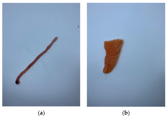
Figure 1.
(a) Tuna and (b) salmon meat samples extracted from fresh fish, to be photographed.
We emphasize that both the tuna and the salmon used were fresh fish. Samples were placed on cards made of white paper and transported to a laboratory to be photographed in the industry/restaurant itself. According to the observation of colourimetric patterns, specialists in tuna and salmon freshness classification labelled each sample at a specific level of freshness. Meat texture, blood on the gills, and odour were also parameters used by experts. The cards favoured the collection since they avoided manipulating the pieces that broke easily. Each card contained only a sample and was placed individually in the studio to be photographed. The total time between the extraction of the sample from the fish body and its image capture took, on average, 3 min. We discarded the pieces after the capture session.
2.2. Computer Vision System
The CVS for capturing images consisted of a studio with thirty-six white and circularly LED lights at the top, with 6500 K. The studio used to acquire the images, shown in Figure 2, prevents sidelight entry since the sample had walls. An iPhone XR smartphone camera was positioned at the top of the studio’s opening, and the height between the camera and pieces was 12.5 cm. The camera was configured without zoom, flash, f/1.8 aperture, optical stabilization, natural lighting, and touch focus. The images were taken on a white background and saved on the smartphone’s camera roll in JPEG format as matrices with dimensions 4608 × 2592 pixels.
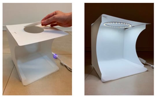
Figure 2.
Studio for sample capture.
2.3. Preprocessing of Images
The computer used to perform the images’ preprocessing consists of a MacBook Pro 2017 notebook, i5 2.3GHz, 32GB of RAM. For image analysis, we used a feature extractor script. Figure 3 shows the image preprocessing steps [20].
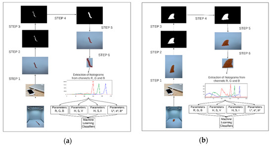
Figure 3.
Image preprocessing steps for (a) tuna and (b) salmon samples. Caption: step 1: resizing the original image to 600 × 400 pixels; step 2: grayscale image, created from the mask that uses a limit for (a) red and (b) orange variations; step 3: grayscale image, generated from Gaussian filter; step 4: binary image generated from thresholding; step 5: contours defined; step 6: cut the contoured area to determine the region of interest.
The script initially resizes images to 600 × 400 pixels to reduce processing and converts the original RGB image to the HSV format. For defining the region of interest in tuna meat samples pictures, the script uses a three-dimensional range of H, S, and V minimum (160, 0, 0) and maximum (180, 255, 255), representing variations of red tones. For the images of salmon meat samples, the range varied from (5, 50, 50) to (15, 255, 255), representing variations in shades of orange, the predominant color in the samples. The script then applies a grayscale mask to the red/orange-coloured pixels found in the range, generating a Gaussian noisy grayscale image.
The primary sources of Gaussian noise in digital images are lighting or high-temperature problems during acquisition, transmission, or processing. In digital image processing, a Gaussian noise can be caused by an abrupt change in an image’s pixel values. Filter techniques are used with the disadvantage of blurring it a little to mitigate noise. The Gaussian filter reduces an input signal’s noise level to reduce distortion in an image [40]. The script applies a Gaussian filter to the Gaussian noisy grayscale image, obtaining blurred vision.
From the blurred image, thresholding is applied to segment the image, creating a binary image. Then, the script analyzes the binary image to define the sample contour. This will find the shape consists of analyzing the binary image’s pixels, and those with 0 are outside of the outline, while pixels with values 1 are inside the design. Again, in RGB format, a picture is obtained with the region of interest outlined. Finally, the script makes a rectangular cut, producing the smallest bounding rectangle possible for the contour, resulting in an area of interest in the image. The script gets the histogram and parameters of the RGB, HSV, HSI, and L*a*b* color spaces from the preprocessed images to use them as predictor variables in classifiers based on ML techniques.
The tuna sample dataset contained ninety-five samples, while the salmon dataset included one hundred and five samples. The two datasets were built in a controlled environment. Using a controlled environment constitutes the first phase of the research, making it possible to quickly test the colourimetric variables extracted from the samples.
As the tuna dataset was the first to be built, we tried to capture the pieces of meat in an uncontrolled environment, encountering difficulties such as the absence of benches in the fish unloading area and the process of removing the fish from non-standard refrigerated trucks. For example, there are situations in which fish are removed from refrigerated and weighed trucks and are punctured with sashibo on the scale itself. The meat is sometimes classified in the hand of the specialist, not favouring photography. In other situations, several fish are punctured with sashibo, and the meat sample is placed over the fish’s body to be classified, which also does not favour photography. The partner industry specialist sometimes used the controlled environment proposed in this research since he had a setting to type the freshness of the meat in a more standardized way. We believe that creating an environment within the industry’s unloading area, which can accommodate the extracted sample and have a lighting and background pattern, can diminish specialists’ inherent subjectivity of classifying tuna. It could mitigate errors or bias. Our perception showed that standardized hardware and capture protocol, of meagre cost, can increase the quality of the specialist’s service during the collection. With the experience of collecting tuna samples, we collected salmon samples directly in the controlled environment.
The two sample datasets columns consist of the parameters of the four studied color spaces. The freshness level labels identified by the specialist have been added.
The tuna tags can denote five classifications of freshness levels when observing colourimetric parameters: #1, #2+, #2, #2−, and #3, in disbelieving order, label #1 represents the classification “most fresh”. Label #3 represents the lowest level of freshness but is still acceptable for consumption. The collection of tuna samples show only levels #2+, #2, #2−, and #3. According to the specialist, tuna with a freshness level #1 is rare.
Ninety-five tuna and fifty salmon samples were analyzed in this study. Salmon classification labels denote only three levels of freshness: “very fresh”, “fresh”, and “immediate consumption”.
The low number of tuna samples was justified by a recent study and the extreme difficulty in the dataset construction process, which relies on fish, the industry routine, and the specialist’s ability to monitor the researchers’ work. The specialist focuses on placing the sashibo samples directly on the white cards to be photographed, and explaining why he labelled the separate piece with a specific classification, causing a delay in the process. Another factor appears in that fishing boats have caught tuna of different species, although the vast majority are Bigeye tuna. However, although Yellowfin tuna were also detected in smaller numbers, we could not collect their samples. Our presence during unloading fish from refrigerated trucks represents a significant change in the industry’s freshness classification process. Fish are usually removed from the refrigerated truck when purchase orders are registered in the industry, often causing us to have access to few samples after sometimes four hours of waiting in an environment without a waiting room and a fishy smell.
The low number of salmon samples is due to a recent study and the reduced amount of fish received by the partner restaurant per week.
Finally, the samples collection process was impacted by SARS-CoV-2 since consumer demand for fresh fish has declined considerably. Restaurants had low customer numbers since Brazil presented with an increase in the contagion curve of SARS-CoV-2. The collection process could have a larger team, but the sanitary measures prevented many people in the industry and the restaurant.
2.4. Color Space Parameters
The script took the RGB color space parameters directly from the histogram images since the camera captures these in RGB format to identify the fish meat’s freshness through color aspects. These parameters represent the intensity of red, green, and blue colors. The script calculated the color spaces HSV, HSI, and L*a*b*.
To form a color with RGB, three light beams (one red, one green, and one blue) must be superimposed, employing the principle of human eye functionality (sensitivity of the retina to three types of specific light spectra). Each of the beams is called a component of that color. Each component has an arbitrary intensity, ranging from 0 to 255. The RGB color model is additive because the three light beams are added together, and their light spectra form the final color spectrum. Red, green, and blue are primary colors because they can produce secondary colors from their combinations. Zero intensity for each component gives the darkest color (black), and the full intensity of each gives the lightest color (white). When the powers for all components are equal, the result is a shade of grey, darker or lighter depending on the intensity. When the forces are different, the result is a colored tint. The primary colors were standardized by the CIE (Commission Internationale de l’Éclairage) in wavelengths: red (700 nm), green (546.1 nm), and blue (435.8 nm) [11].
The hue saturation value (HSV) color space was created by Alvy Ray Smith in 1978. Commonly used in CV applications, the HSV color space is formed by the components H (hue), S (saturation), and V (value). The H component, called hue, can be understood as the hue of the color; it measures the dominant wavelength of the color and can be interpreted as the distance to red. Their values vary around the vertical axis of a hex cone, measured in degrees, ranging from 0 to 360. The hex cone represents the graph of the HSV color space. The S component or saturation, also called “purity”, has 0 to 100% values. The smaller this value, the more gray the image will be (less pure), while the higher the value, the more “pure” the image. Finally, the V component, or value, is analogous to the brightness/light of the color, also ranging between 0% and 100% [11].
The hue saturation intensity (HSI) space was created to allow another form of image processing. The HSI color space separates intensity I from H (hue) and S (saturation). The H and S components of the HSI color space represent similar concepts to the H and S components of the HSV color space. At the same time, the I value of HSI embodies the achromatic notion of intensity, being similar to brightness in HSV. However, the equations that convert RGB components to HSI differ from those that convert RGB to HSI. The graphical representation of the HSI is a bicone (two cones) joined by the base [12].
In general, colors differ in chromaticity and luminance. The parameters of the L*a*b* color space created by the CIE correlate color values with visual perception. This color space was created based on the Opposite Color Theory [41], in which two colors cannot be green and red at the same time or yellow and blue at the same time. The L* parameter indicates brightness, and the a* and b* parameters represent the chromatic coordinates, with a* being the red/green coordinate (+a indicates red and −a indicates green) and b* the yellow/blue coordinate (+b indicates yellow and −b indicates blue) [13].
Following CIE guidelines, in which L*a*b* is one of the spaces for comparing different colors, industries with plastic, ink, printing, food, and textile industries use this space to identify product color attributes and deviations from a standard color. Small differences can be found by a color measuring instrument, even when two colors look the same to one person. Color differences are defined by the numerical comparison between the sample and the standard [42].
To convert RGB values to L*a*b*, RGB components must be linearized concerning light [13]. To do so, we convert RGB components into XYZ components of the CIE XYZ color space [43], and then convert the XYZ components into the L*a*b* color space components using the D65 illuminant values.
The script automatically extracts the bands R, G, and B from the histogram when the image’s region of interest is defined. Three features are extracted for R, G, and B bands: the means of all histogram pixels. Then, the images are converted from RGB to HSV, HSI, and L*a*b*. The respective means of the histogram parameters are extracted through all pixels, generating nine more features in the dataset. Six more features are removed from the HSV color space: means of the pixels of the peak histogram and the median of the ridge of the histogram of the H, S, and V channels. In total, eighteen features are available in the dataset to be analyzed by classification models.
3. Color Features and AutoML
This section will discuss features extracted from samples based on colorimetric patterns and the AutoML method used to test the ML model.
3.1. Color Features
We begin the discussion by analyzing the feature correlation matrix of the datasets shown in Figure 4.
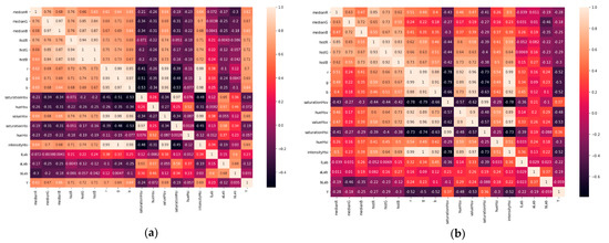
Figure 4.
Correlation matrix of extracted features based on colors of (a) tuna and (b) salmon meat samples.
The features r, g, b represent the mean of all histogram points for channels R, G, and B. The saturationHsv, hueHsv, valueHsv features represent the saturation, hue, and value values of the HSV color space. Using values above 150 of the saturationHsv parameter, we calculate the peak of the HSV histogram for tones of red (for tuna samples) and tones of orange (for salmon samples). We emphasize that saturation values above 150 represent strong tones of the color in question since saturation can be understood as the intensity of the color. Features histR, histG, and histB represent the peak of the histogram of channels H, S, and V. Features medianR, medianG, and medianB represent the median of the previous histograms. The saturationHSI, hueHSI, and intensityHsi features represent the HSI color space’s saturation, hue, and intensity values. Finally, the features lLab, aLab, and bLab represent L*a*b* color space values. The analysis of the correlation matrices presented in Figure 4 shows a strong correlation (above 90%), giving us the certainty that information redundancy disrupts the models, since they are subject to duplicated information that is not always useful for learning model. The monotony of data suggests applying preprocessing feature techniques so that ML models do not have higher computational costs for training. Quickly finding the best feature preprocessing method to deliver the ideal datasets so that classifiers are trained and generate good classification models becomes challenging, given the number of combinations that can be made, which justifies our choice to use AutoML.
We see in Figure 5 the number of samples in each class or freshness level. We can see in Figure 5a that there are a different number of samples for each class, with the dataset of unbalanced tuna samples. Tuna freshness levels, being categorical variables, were coded into numerical variables: level 2− was coded as 0, level 3 was coded as 1, level 2 was coded as 2, and level 2+ was coded similar to 3. Class 0 is the majority, while class 2 is the minority.
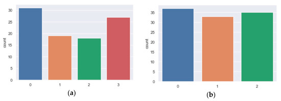
Figure 5.
Number of samples by freshness level of (a) tuna and (b) salmon.
The dataset of salmon samples is also unbalanced, as shown in Figure 5b, where class 0 is the majority and class 1 is the minority. Class 0 represents the lowest freshness level, labelled “immediate consumption”. Class 1 represents the label “fresh”, and finally, class 2 represents the class with the highest level of freshness, labelled “very fresh”.
We use the uniform manifold approximation and projection (UMAP) dimensionality reduction technique [44] to understand how the proposed feature choice is adequate to classify the freshness of tuna and salmon meat. Any other dimensionality reduction technique could have been used. The purpose of using a dimensionality reduction technique is to make it possible to visualize, in a two-dimensional orthogonal cartesian axis, whether the existing classes in the dataset form a well-defined cluster, and the UMAP technique is suitable for this purpose.
In Figure 6, we see that UMAP has successfully captured the four tuna meat freshness classes existing in the dataset. We can also observe that the freshness classifications are dismissed as clearly distinct. Only two samples with legend 0 appear further away from their true cluster and may be samples of mixed freshness. As with the tuna freshness classes, UMAP successfully captured the three freshness levels of salmon meat, as shown in Figure 6b. The clustering graphs in Figure 6 prove that the features proposed to classify tuna meat freshness levels are also suitable for organizing salmon meat freshness levels. We understand that such features can be applied to other food products. The clustering graph in Figure 6 proves the adequacy of the features proposed in this paper for evaluating colorimetric patterns of tuna meat freshness.
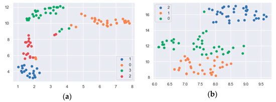
Figure 6.
Tuna (a) and salmon (b) class clustering graph generated by the UMAP technique.
3.2. AutoML
We understand the need for CVS validation through ML methods. There are several algorithm classifiers of ML. Defining the parameters that must be used during the execution of each algorithm to control the training process and ensure the best results is computationally expensive and may discourage further experiments, as each problem behaves in a specific way. We used an AutoML method to reduce the costs in the development process and tested many classifiers in conjunction with preprocessing, feature preprocessing, and balancing techniques. We understand that generated AutoML models that present good metrics encourage the use of CVS in other contexts, attempts to increase datasets of tuna and salmon samples, and above all, the development of new classification models.
AutoML refers to techniques for automatically discovering well-performing models for predictive modelling tasks with very little user involvement. AutoML improves ML efficiency and accelerates the research. The AutoML pipeline allows for automating the preprocess, cleaning the data, selecting and constructing appropriate features, selecting a proper model family, optimizing model hyperparameters, post-process ML models, and critically analyzing the results [45].
In this study, we chose to use the Auto-Sklearn framework [46], an open-source library written in Python. It makes use of the popular Scikit-Learn machine learning library for data transforms and ML algorithms. It uses a Bayesian Optimization search procedure to discover a top-performing model pipeline for a given dataset efficiently.
The benefit of Auto-Sklearn is that in addition to discovering the data preparation and model that performs best for a dataset, it can learn from models that performed well on similar datasets and automatically create an ensemble of top-performing models discovered as part of the optimization process [46].
We performed a random dataset split in the classification process, considering 80% for training data and 20% for test data. The training base had 76 samples in the tuna dataset, while the test base had 19 pieces. The training base consists of 84 examples in the salmon dataset and the test base of 21 selections.
Cross-validation [47] with ten folders was performed in the training data, and we made predictions using test data to check the accuracy and ROC_AUC of the models in the pipeline. The execution time of tuning for each pipeline was specified as 720 s.
4. Results and Discussion
To analyze freshness levels, we use PipelineProfiler [48], a tool that enables the interactive exploration of pipelines generated by AutoML systems. Figure 7 and Figure 8 show the PipelineProfiler that applied the tuna and salmon samples dataset to the AutoML system, respectively, to compare different pipelines that predict freshness levels. The main components of PipelineProfiler are the primitives (A), the pipeline matrix (B), and the pipeline comparison view (C), shown in Figure 7 and Figure 8.
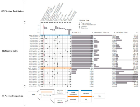
Figure 7.
PipelineProfiler applied to the analysis of tuna meat classification pipelines generated by the AutoML system.
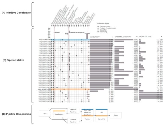
Figure 8.
PipelineProfiler applied to the analysis of salmon meat classification pipelines generated by AutoML systems.
The pipeline matrix models the pipelines as a set of primitives that can be effectively displayed in a matrix to summarize a collection of pipelines concisely. The pipeline matrix shows a tabular summary of all the pipelines in the pool. The pipeline comparison view consists of a node-link diagram that offers either an individual pipeline or a visual-difference overview of multiple pipelines selected in the matrix representation. Each primitive (node) is color-coded in the summary graph to indicate the pipeline where it appears. If a primitive is present in multiple pipelines, all corresponding colors are displayed. If a primitive appears in all selected pipelines, no color is displayed.
To compare pipeline patterns, we sought to identify common patterns in the best pipelines in the PipelineProfiler. To this end, we first sorted the primitives by type and the pipelines by performance. This was useful to uncover patterns.
As we saw in Figure 5, the tuna and salmon sample datasets are unbalanced. In cases of unbalanced dataset predictions, minority classes may never be predicted, even in models with high accuracy [6]. In this study, we need the minority class of tuna (class 2) and salmon (class 1) to be accurately predicted, as fish’s commercial values and shelf-life change depending on these classifications, justifying the importance of class balancing techniques. To do so, we used one approach to address the imbalanced training dataset to oversample the minority class to train AutoML models. The approach involves duplicating examples in the minority class, although these examples do not add any new information to the model. Instead, recent examples can be synthesized from the existing samples. It consists of a technique of data augmentation for the minority class and is referred to as the synthetic minority oversampling technique (SMOTE) [49]. We will not evaluate the class balancing primitive in PipelineProfiler. We emphasize that we generated the AutoML model without class balancing and other techniques, with the SMOTE technique being the one that obtained the best values of the evaluated metrics.
We evaluated the AutoML models to classify the freshness levels of tuna and salmon samples through the metrics: accuracy [50], receiver operating characteristic (ROC) curve [51], precision [52], recall [53], f1-score [54], and confusion matrix (CM) [55].
Accuracy is the proportion of the total number of correct predictions [50]; the ROC curve is a graph showing the performance of a classification model at all classification thresholds. This curve plots two parameters: true positive rate and false-positive rate [51]. Precision is the fraction of relevant instances among retrieved instances [52], while recall is the fraction of retrieved cases [53]. The f1-score combines recall with accuracy so that they bring a single number [54]. Finally, a confusion matrix is a specific table layout that allows visualization of the performance of an algorithm. Each row of the matrix represents the instances in an actual class, while each column represents the instances in a predicted class, or vice versa [55].
We first analyzed the PipelineProfiler generated from the tuna dataset, shown in Figure 7. Thirty-two pipelines were analyzed; eight exceeded the 720 s time limit set for the tuning. We can see that 100% of the pipelines presented the categorical transformer [56] and numerical transformer [56] techniques in the preprocessing primitives.
To build a classification pipeline for identifying the freshness of tuna meat, we evaluate different ML classifiers: Random Forest (RF) [57], Passive Aggressive (PA) [58], Extra Tree [59], Linear Discriminant Analysis (LDA) [60], Library Support Vector Machine (libsvm_svc) [61], Multilayer Perceptron (MLP) [62], Stochastic Gradient Descent (SGD) [63], Quadric Discriminant Analysis (QDA) [64], Gradient Boosting (GB) [65], and Ensemble [66] methods, combined with preprocessing, feature preprocessor, and balancing techniques.
Without loss of understanding, we will call the Ensemble model, the set of pipelines chosen by AutoML to classify the freshness of samples.
In Figure 7, we see the pipelines, accuracy, weights in the Ensemble, and mean fit time. The pipelines #2, #6, #9, #14, #17, #18, #22, #23, #24, #25, #26, #27, #28, #29, #30, #31, and #32 were out of the Ensemble, even with some of them showing high accuracy, which leads us to conclude that Auto-Sklearn uses other criteria to assign weights to pipelines in the Ensemble. Pipelines #25, #26, #27, #28, #29, #30, #31, and #32 exceeded the established processing time limit. Pipelines #1 and #21 had the greatest weight in the Ensemble and are highlighted in the pipeline comparison section (C) in Figure 7. Pipeline #1, blue node, presents a feature agglomeration technique as a feature preprocessing primitive and libsvm_svc classifier. Pipeline #21 presents a feature polynomial technique as a feature preprocessing primitive and SGD classifier. We noticed that the pipelines that presented greater mean fit time have SG as a classifier.
Table 2 shows the Ensemble model metrics generated by AutoML. The accuracy, precision, recall, and f1-Score have maximum values (optimal values) equal to 100%, demonstrating exceptional results. Support values represent the numbers of samples in each class.

Table 2.
Ensemble model metrics for sorting tuna samples.
The ROC curve is shown in Figure 9. The area under the curve of the four classes representing the freshness of tuna meat equals 1.0, corroborating that the model assertively predicts 100% of the classes.
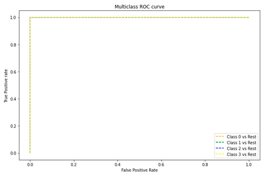
Figure 9.
ROC curve graph of the classes that represent the freshness of tuna meat.
The feature importance graph is shown in Figure 10. The hueHSI feature was considered the most relevant for the Ensemble, followed by the hueHSV feature. The histR and B features were considered equally important to the Ensemble, having less relevance than the previous ones. The other features were not important.
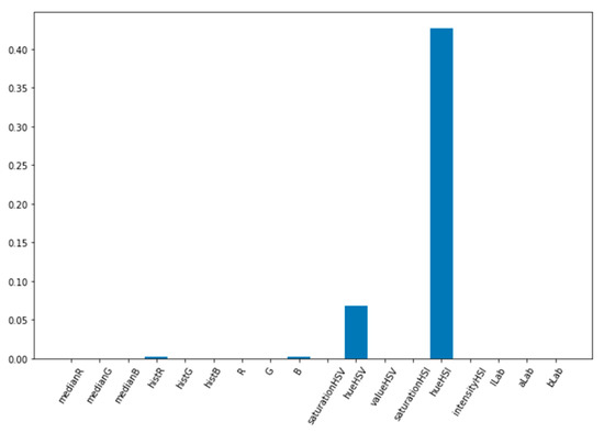
Figure 10.
Feature importance graph for the Ensemble model generated by AutoML for tuna meat freshness classification.
To illustrate how well-used the class balancing techniques were, we generated the CM from a prediction made by the Ensemble for freshness tuna classification, Figure 11. We realized that 100% of the samples were classified assertively.
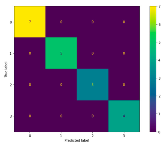
Figure 11.
Confusion matrix of tuna sample prediction performed by Ensemble.
For salmon classification, AutoML generated thirty-six pipelines, as shown in Figure 8. The RF, LDA, Adaboost [67], libsvm_svc, Extra Tree, PA, KNN, MLP, Decision Tree (DT) [68], Bernoulli naïve Bayes (bernoulli_nb) [69], and GB classifiers were tested. Pipelines #3, #4, #20, #22, #30, #31, #32, #33, #34, #35, and #36 were left out of the Ensemble. We highlight that pipelines #3, #4, #20, and #22 were out of the Ensemble, even with high accuracy. Pipeline #30 had low accuracy, while pipelines #31, #32, #33, #34, #35, and #36 had a processing time greater than the established limit and were not considered in the Ensemble. Pipelines #1 and #29 were considered the most important in the Ensemble and are highlighted in section (C) of Figure 8. Pipeline #1, blue nodes, presented with the Extra Tree technique as a primitive feature preprocessor and MLP classifier. Pipeline #29, orange nodes, presented the fast_ica technique as a primitive feature preprocessor classifier bernoulli_nb. We realize that the biggest mean fit time is linked to the GB classifier.
The precision, recall, f1-score, and accuracy metrics of the AutoML-generated Ensemble for salmon freshness rating are shown in Table 3. As with the tuna dataset metrics, the salmon dataset is displayed at its’ maximum values, the best possible values, showing how easy it was to extend the proposed CVS to another context.

Table 3.
Ensemble model metrics for sorting salmon samples.
The ROC curve shown in Figure 12 presents an area value equal to 1.0 for all classes of salmon freshness levels, corroborating the excellent results of the Ensemble.
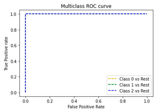
Figure 12.
ROC curve graph of the classes that represent the freshness of salmon meat.
The feature importance graph shown in Figure 13 highlights that the peaks of the HSV histogram, represented by the histR, histG, and histB features, are extremely relevant for the Ensemble, with the histR feature being the most pertinent. Feature R also has central importance, and finally feature G and intensityHSI appear in the chart, but to lesser extent than those mentioned. The other features appear without relevance.
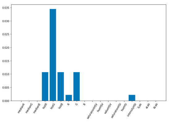
Figure 13.
Feature importance graph for the Ensemble model generated by AutoML for salmon meat freshness classification.
Finally, to illustrate the relevance of applying class balancing techniques and mitigate the possibility that minority classes could be misclassified, we present in Figure 14 the CM of the prediction made by the Ensemble for the classification of salmon freshness. The samples were assertively classified in their entirety.
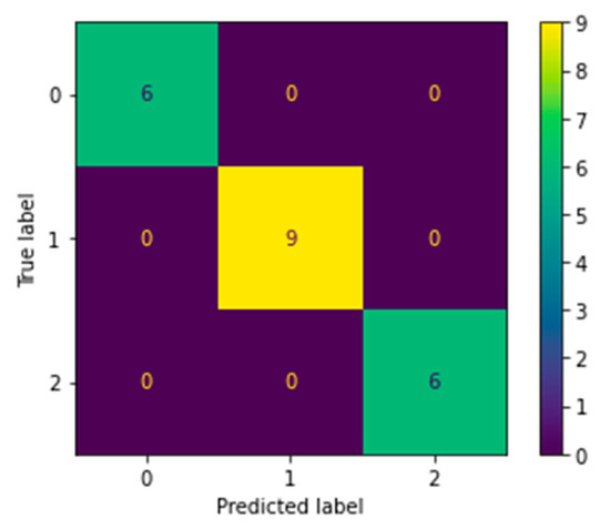
Figure 14.
Confusion matrix of salmon sample prediction performed by Ensemble.
5. Conclusions
This paper describes a CV solution for tuna and salmon meat samples’ freshness classification. The CVS provides a useful CV application combined with ML methods to estimate tuna freshness in four categories, and the freshness of salmon in three categories. The system includes image acquisition, preprocessing techniques, extraction of characteristics from color spaces, and classification using AutoML. We use Auto-Sklearn to quickly and reliably find the best combinations of preprocessing, feature preprocessor, and balancing techniques, as well as classifiers to classify tuna and salmon meat freshness through colorimetric parameters extracted from meat sample images. To analyze freshness levels, we used the PipelineProfiler, which enables the interactive exploration of pipelines generated by AutoML systems.
As the datasets of tuna and salmon samples were unbalanced, and given the importance of assertively classifying minority classes, we chose to use the SMOTE technique to balance the classes due to the commercial value of the fish. We noticed that 100% of pipelines used numeric and categorical transformations as the preprocessing primitive.
For tuna classification, thirty-two pipelines were analyzed; four exceeded the 720 s time limit set for the tuning. Eight pipelines were dropped out of the Ensemble for exceeding the 720 s processing limit.
The Ensemble generated by AutoML was composed of pipelines #1 (libsvm_svc classifier), #3 (RF classifier), #4 (RF classifier), #5 (libsvm_svc classifier), #7 (RF classifier), #8 (RF classifier), #10 (PA classifier), #11 (QDA classifier), #12 (LDA classifier), #13 (RF classifier), #15 (RF classifier), #16 (RF classifier), #19 (MLP classifier), #20 (MLP classifier), #21 (SGD classifier). Pipelines #1 and #21 had the greatest weights in the composition of the Ensemble. In total, 100% of the pipelines used numerical and categorical transformation techniques in the preprocessing primitive.
The metrics used to evaluate Ensemble’s performance for tuna classification were accuracy, ROC curve, precision, recall, f1-score, and confusion matrix (CM). All metrics presented values equal to 100% assertiveness, an excellent result demonstrating the adequacy of the CVS built for the task of classifying tuna meat freshness.
We used the same method to rate salmon freshness with the encouraging results obtained in the tuna experiment and to check whether CVS could easily be used in other grading contexts using color standards. As we did with the tuna experiment, we also used the SMOTE technique as class balancing. The AutoML tested thirty-six pipelines and generated an Ensemble composed of twenty-five pipelines, obtaining accuracy, ROC curve, precision, recall, f1-score, and confusion matrix (CM) metrics at their maximum values, with 100% assertiveness, demonstrating the power of CVS and ease of use in other contexts. Six pipelines passed the 720 s processing limit. One hundred per cent of the pipelines used numerical and categorical transformation techniques in the preprocessing primitive. The pipelines that make up the Ensemble are #1 (MLP classifier), #2 (MLP classifier), #5 (LDA classifier), #6 (MLP classifier), #7 (MLP classifier), #8 (MLP classifier), # 9 (RF classifier), #10 (Extra Tree classifier), #11 (RF classifier), #12 (RF classifier), #13 (RF classifier), #14 (MLP classifier), #15 (RF classifier), # 16 (RF classifier), #17 (RF classifier), #18 (RF classifier), #19 (RF classifier), #21 (PA classifier), #23 (KNN classifier), #24 (LDA classifier), #25 (DT classifier), #26 (MLP classifier), #27 (MLP classifier), #28 (MLP classifier), and #29 (bernoulli_nb classifier). Pipelines #1 and #29 were the ones with the greatest weight in the Ensemble. The presence of the GB classifier in the pipeline was associated with a greater mean fit time.
Comparing the accuracy metric of our work with all the results listed in Table 1, none of them reaches 100%, noting that our CVS can represent an alternative for testing in the contexts of related works. Comparing our research with previous work specifically related to tuna classification, Lugatiman, Fabiana, Echavia, and Adtoon. [36] presented a KNN-based solution with 86.6% accuracy. Moon, Kim, Xu, Na, Giaccia, and Lee [37] proposed a CNN for the same task, obtaining an accuracy of 88%. For the classification of salmon freshness, the authors. achieved an accuracy of 84% for Atlantic salmon and 85% for Pacific salmon. Our research presents classification models with greater accuracy than the studies [36,37].
We emphasize that we are not comparing the sample collection protocol and extracting features from the images in our study with the studies [36,37]. However, we understand that these approaches directly affect the quality of the constructed classification models. We are just presenting an alternative CVS model to the CVS models of Lugatiman et al. and Moon et al., after an exhaustive combination of data preprocessing, feature preprocessor, classifiers, and balancing results models with greater accuracy.
The main contributions of this research stand out: construction of a controlled environment for sample collection that can be implemented to standardize the classification of the samples by the specialist; an easily extendable script extractor feature for other food contexts; and the analysis of several ML models for a variety of tuna and salmon meat freshness. We concluded that the development of hardware and protocol for image collection, datasets with color pattern information, and ML models’ application could be considered reliable, fast, and nondestructive to classify tuna and salmon meat extracted using sashibo.
Limitations were the low amount of tuna and salmon meat samples, emphasizing this as a recent study. Data collection is dependent on the availability of fish and the access that the industry and restaurant allow us. For future assignments, we suggest tests with more samples and with models not covered by AutoML. DL approaches will be considered as soon as a dataset containing a larger volume of samples is available.
Author Contributions
Conceptualization, E.C.M., L.M.A. and J.G.d.A.T.F.; methodology, E.C.M., L.M.A. and J.G.d.A.T.F.; software, E.C.M. and L.M.A.; validation, E.C.M., L.M.A. and J.G.d.A.T.F.; formal analysis, E.C.M.; investigation, E.C.M.; resources, E.C.M., L.M.A. and J.G.d.A.T.F.; data curation, E.C.M.; writing—original draft preparation, E.C.M.; writing—review and editing, E.C.M., L.M.A. and J.G.d.A.T.F.; visualization, E.C.M., L.M.A. and J.G.d.A.T.F.; supervision, L.M.A. and J.G.d.A.T.F.; project administration, L.M.A. and J.G.d.A.T.F. All authors have read and agreed to the published version of the manuscript.
Funding
This research received no external funding.
Institutional Review Board Statement
Not Applicable.
Informed Consent Statement
Not Applicable.
Data Availability Statement
Images and scripts for automatic generation of datasets containing color features are available at https://github.com/erikamedeiros/informatics.
Conflicts of Interest
The authors declare no conflict of interest.
References
- Sun, D.-W. Computer Vision Technology for Food Quality Evaluation; Academic Press: Cambridge, MA, USA, 2016. [Google Scholar]
- Olafsdottir, G.; Martinsdóttir, E.; Oehlenschläger, J.; Dalgaard, P.; Jensen, B.; Undeland, I.; Mackie, I.M.; Henehan, G.; Nielsen, J.; Nilsen, H. Methods to evaluate fish freshness in research and industry. Trends Food Sci. Technol. 1997, 8, 258–265. [Google Scholar] [CrossRef]
- Dutta, M.K.; Issac, A.; Minhas, N.; Sarkar, B. Image processing based method to assess fish quality and freshness. J. Food Eng. 2016, 177, 50–58. [Google Scholar] [CrossRef]
- Bremner, H.A.; Sakaguchi, M. A critical look at whether freshness can be determined. J. Aquat. Food Prod. Technol. 2000, 9, 5–25. [Google Scholar] [CrossRef]
- Szeliski, R. Computer Vision: Algorithms and Applications; Springer Science & Business Media: Berlin/Heidelberg, Germany, 2010. [Google Scholar]
- Alpaydin, E. Introduction to Machine Learning; MIT Press: Cambridge, MA, USA, 2020. [Google Scholar]
- Brosnan, T.; Sun, D.-W. Inspection and grading of agricultural and food products by computer vision systems—A review. Comput. Electron. Agric. 2002, 36, 193–213. [Google Scholar] [CrossRef]
- Gümüş, B.; Balaban, M.Ö.; Ünlüsayin, M. Machine vision applications to aquatic foods: A review. Turk. J. Fish. Aquat. Sci. 2011, 11, 167–176. [Google Scholar] [CrossRef]
- Hanson, A. Computer Vision Systems; Elsevier: Amsterdam, The Netherlands, 1978. [Google Scholar]
- Süsstrunk, S.; Buckley, R.; Swen, S. Standard RGB color spaces. In Color and Imaging Conference; Society for Imaging Science and Technology: Springfield, VA, USA, 1999; Volume 1999, pp. 127–134. [Google Scholar]
- Milligan, P.R.; Morse, M.P.; Rajagopalan, S. Pixel map preparation using the HSV color model. Explor. Geophys. 1992, 23, 219–223. [Google Scholar] [CrossRef]
- Welch, E.; Moorhead, R.; Owens, J.K. Image processing using the HSI color space. In Proceedings of the IEEE Proceedings of the SOUTHEASTCON91, Williamsburg, VA, USA, 7–10 April 1991; pp. 722–725. [Google Scholar] [CrossRef]
- Connolly, C.; Fleiss, T. A study of efficiency and accuracy in the transformation from RGB to CIELAB color space. IEEE Trans. Image Process. 1997, 6, 1046–1048. [Google Scholar] [CrossRef] [PubMed]
- He, X.; Zhao, K.; Chu, X. AutoML: A survey of the state-of-the-art. Knowl. Based Syst. 2021, 212, 106622. [Google Scholar] [CrossRef]
- Trientin, D.; Hidayat, B.; Darana, S. Beef freshness classification by using color analysis, multi-wavelet transformation, and artificial neural network. In Proceedings of the 2015 International Conference on Automation, Cognitive Science, Optics, Micro Electro-Mechanical System, and Information Technology (ICACOMIT), Bandung, Indonesia, 29–30 March 2015; pp. 181–185. [Google Scholar] [CrossRef]
- Kramer, O. K-nearest neighbors. In Dimensionality Reduction with Unsupervised Nearest Neighbors; Springer: Berlin/Heidelberg, Germany, 2013; pp. 13–23. [Google Scholar] [CrossRef]
- Hopfield, J.J. Artificial neural networks. IEEE Circuits Devices Mag. 1988, 4, 3–10. [Google Scholar] [CrossRef]
- Jang, E.; Cho, H.; Kim, E.K.; Kim, S. Grade Prediction of Meat Quality in Korean Native Cattle Using Neural Network. In Proceedings of the 2015 International Conference on Fuzzy Theory and Its Applications (iFUZZY), Yilan, Taiwan, 18–20 November 2015; pp. 28–33. [Google Scholar] [CrossRef]
- Adi, K.; Pujiyanto, S.; Nurhayati, O.D.; Pamungkas, A. Beef Quality Identification Using Color Analysis and K-Nearest Neighbor Classification. In Proceedings of the 2015 4th International Conference on Instrumentation, Communications, Information Technology, and Biomedical Engineering (ICICI-BME), Bandung, Indonesia, 2–3 November 2015; pp. 180–184. [Google Scholar] [CrossRef]
- Gonzalez, R.; Woods, R.; Eddins, S. Digital Image Processing Using MATLAB, 3rd ed.; Gatesmark: Knoxville, TN, USA, 2020. [Google Scholar]
- Winiarti, S.; Azhari, A.; Agusta, K.M. Determining feasibility level of beef quality based on histogram and k-means clustering. In Proceedings of the 2018 International Symposium on Advanced Intelligent Informatics (SAIN), Yogyakarta, Indonesia, 29–30 August 2018; pp. 195–198. [Google Scholar] [CrossRef] [Green Version]
- Altini, N.; De Giosa, G.; Fragasso, N.; Coscia, C.; Sibilano, E.; Prencipe, B.; Hussain, S.M.; Brunetti, A.; Buongiorno, D.; Guerriero, A.; et al. Segmentation and identification of vertebrae in CT scans using CNN, k-means clustering and k-NN. Informatics 2021, 8, 40. [Google Scholar] [CrossRef]
- Hamerly, G.; Elkan, C. Learning the k in k-means. Adv. Neural Inf. Process. Syst. 2004, 16, 281–288. [Google Scholar]
- Arsalane, A.; El Barbri, N.; Tabyaoui, A.; Klilou, A.; Rhofir, K.; Halimi, A. An embedded system based on DSP platform and PCA-SVM algorithms for rapid beef meat freshness prediction and identification. Comput. Electron. Agric. 2018, 152, 385–392. [Google Scholar] [CrossRef]
- Bro, R.; Smilde, A.K. Principal component analysis. Anal. Methods 2014, 6, 2812–2831. [Google Scholar] [CrossRef] [Green Version]
- Sánchez, A.V.D. Advanced support vector machines and kernel methods. Neurocomputing 2003, 55, 5–20. [Google Scholar] [CrossRef]
- Hosseinpour, S.; Ilkhchi, A.H.; Aghbashlo, M. An intelligent machine vision-based smartphone app for beef quality evaluation. J. Food Eng. 2019, 248, 9–22. [Google Scholar] [CrossRef]
- Tan, W.K.; Husin, Z.; Ismail, M.A.H. Feasibility study of beef quality assessment using computer vision and Deep Neural Network (DNN) algorithm. In Proceedings of the 2020 8th International Conference on Information Technology and Multimedia (ICIMU), Selangor, Malaysia, 24–26 August 2020; pp. 243–246. [Google Scholar] [CrossRef]
- Goodfellow, I.; Bengio, Y.; Courville, A. Deep Learning; MIT Press: Cambridge, MA, USA, 2016. [Google Scholar]
- Wang, Y.; Friderikos, V. A survey of deep learning for data caching in edge network. Informatics 2020, 7, 43. [Google Scholar] [CrossRef]
- Taheri-Garavand, A.; Fatahi, S.; Shahbazi, F.; de la Guardia, M. A nondestructive intelligent approach to real-time evaluation of chicken meat freshness based on computer vision technique. J. Food Process. Eng. 2019, 42, e13039. [Google Scholar] [CrossRef]
- Wirsansky, E. Hands-on Genetic Algorithms with Python: Applying Genetic Algorithms to Solve Real-World Deep Learning and Artificial Intelligence Problems; Packt Publishing Ltd.: Birmingham, UK, 2020. [Google Scholar] [CrossRef]
- Sun, X.; Young, J.; Liu, J.H.; Chen, Q.; Newman, D. Predicting pork color scores using computer vision and support vector machine technology. Meat Muscle Biol. 2018. [Google Scholar] [CrossRef]
- Taheri-Garavand, A.; Fatahi, S.; Banan, A.; Makino, Y. Real-time nondestructive monitoring of common carp fish freshness using robust vision-based intelligent modeling approaches. Comput. Electron. Agric. 2019, 159, 16–27. [Google Scholar] [CrossRef]
- Karaboga, D.; Akay, B. A comparative study of artificial bee colony algorithm. Appl. Math. Comput. 2009, 214, 108–132. [Google Scholar] [CrossRef]
- Lugatiman, K.; Fabiana, C.; Echavia, J.; Adtoon, J.J. Tuna meat freshness classification through computer vision. In Proceedings of the 2019 IEEE 11th International Conference on Humanoid, Nanotechnology, Information Technology, Communication and Control, Environment, and Management (HNICEM), Laoag, Philippines, 29 November–1 December 2019; pp. 1–6. [Google Scholar] [CrossRef]
- Moon, E.J.; Kim, Y.; Xu, Y.; Na, Y.; Giaccia, A.J.; Lee, J.H. Evaluation of salmon, tuna, and beef freshness using a portable spectrometer. Sensors 2020, 20, 4299. [Google Scholar] [CrossRef]
- Albawi, S.; Mohammed, T.A.; Al-Zawi, S. Understanding of a convolutional neural network. In Proceedings of the 2017 International Conference on Engineering and Technology (ICET), Antalya, Turkey, 21–23 August 2017; pp. 1–6. [Google Scholar] [CrossRef]
- Howse, J. OpenCV Computer Vision with Python; Packt Publishing Ltd.: Birmingham, UK, 2013. [Google Scholar]
- Jain, A.; Gupta, R. Gaussian Filter Threshold Modulation for Filtering Flat and Texture Area of an Image. In Proceedings of the 2015 International Conference on Advances in Computer Engineering and Applications, Ghaziabad, India, 19–20 March 2015; pp. 760–763. [Google Scholar] [CrossRef]
- Jameson, D.; Hurvich, L.M. Some quantitative aspects of an opponent-colors theory. I. Chromatic responses and spectral saturation. JOSA 1955, 45, 546–552. [Google Scholar] [CrossRef]
- Melgosa, M. Testing CIELAB based Color difference Formulas. Color Res. Appl. 2000, 25, 49–55. [Google Scholar] [CrossRef]
- Li, X.W. Research on color space conversion model between XYZ and RGB. In Key Engineering Materials; Trans Tech Publications Ltd.: Freienbach, Switzerland, 2010; Volume 428, pp. 466–469. [Google Scholar] [CrossRef]
- Allaoui, M.; Kherfi, M.L.; Cheriet, A. Considerably improving clustering algorithms using UMAP dimensionality reduction technique: A comparative study. In International Conference on Image and Signal Processing; Springer: Cham, Switzerland, 2020; pp. 317–325. [Google Scholar] [CrossRef]
- Brownlee, J. Auto-Sklearn for Automated Machine Learning in Python. Available online: https://machinelearningmastery.com/auto-sklearn-for-automated-machine-learning-in-python/ (accessed on 4 March 2021).
- Feurer, M.; Klein, A.; Eggensperger, K.; Springenberg, J.T.; Blum, M.; Hutter, F. Auto-sklearn: Efficient and robust automated machine learning. In Automated Machine Learning; Springer: Cham, Switzerland, 2019; pp. 113–134. [Google Scholar]
- Rodriguez, J.D.; Perez, A.; Lozano, J.A. Sensitivity analysis of k-fold cross validation in prediction error estimation. IEEE Trans. Pattern Anal. Mach. Intell. 2009, 32, 569–575. [Google Scholar] [CrossRef] [PubMed]
- Ono, J.P.; Castelo, S.; Lopez, R.; Bertini, E.; Freire, J.; Silva, C. Pipelineprofiler: A visual analytics tool for the exploration of automl pipelines. IEEE Trans. Vis. Comput. Graph. 2020, 27, 390–400. [Google Scholar] [CrossRef] [PubMed]
- Chawla, N.V.; Bowyer, K.W.; Hall, L.O.; Kegelmeyer, W.P. SMOTE: Synthetic minority over-sampling technique. J. Artif. Intell. Res. 2002, 16, 321–357. [Google Scholar] [CrossRef]
- Carvalho, D.V.; Pereira, E.M.; Cardoso, J.S. Machine learning interpretability: A survey on methods and metrics. Electronics 2019, 8, 832. [Google Scholar] [CrossRef] [Green Version]
- Marzban, C. The ROC curve and the area under it as performance measures. Weather Forecast. 2004, 19, 1106–1114. [Google Scholar] [CrossRef]
- Bonnin, R. Machine Learning for Developers: Uplift Your Regular Applications with the Power of Statistics, Analytics, and Machine Learning; Packt Publishing Ltd.: Birmingham, UK, 2017. [Google Scholar]
- Bonaccorso, G. Machine Learning Algorithms; Packt Publishing Ltd.: Birmingham, UK, 2017. [Google Scholar]
- Weiming, J.M. Mastering Python for Finance: Implement. Advanced State-of-the-Art Financial Statistical Applications Using Python; Packt Publishing Ltd.: Birmingham, UK, 2019. [Google Scholar]
- Susmaga, R. Confusion matrix visualization. In Intelligent Information Processing and Web Mining; Springer: Berlin/Heidelberg, Germany, 2004; pp. 107–116. [Google Scholar] [CrossRef]
- Zdravevski, E.; Lameski, P.; Kulakov, A. Advanced transformations for nominal and categorical data into numeric data in supervised learning problems. In Proceedings of the 10th Conference for Informatics and Information Technology (CIIT), Bitola, North Macedonia, 18–21 April 2013. [Google Scholar]
- Breiman, L. Random forests. Mach. Learn. 2001, 45, 5–32. [Google Scholar] [CrossRef] [Green Version]
- Chang, C.-C.; Lee, Y.-J.; Pao, H.-K. A Passive-aggressive algorithm for semi-supervised learning. In Proceedings of the 2010 International Conference on Technologies and Applications of Artificial Intelligence, Hsinchu, Taiwan, 18–20 November 2010; pp. 335–341. [Google Scholar] [CrossRef]
- Brownlee, J. Machine Learning Mastery with Python: Understand Your Data, Create Accurate Models, and Work Projects End-to-End; Machine Learning Mastery: San Francisco, CA, USA, 2016. [Google Scholar]
- Balakrishnama, S.; Ganapathiraju, A. Linear discriminant analysis-a brief tutorial. Inst. Signal Inf. Process. 1998, 18, 1–8. [Google Scholar]
- Chang, C.-C.; Lin, C.-J. LIBSVM: A library for support vector machines. ACM Trans. Intell. Syst. Technol. 2011, 2, 1–27. [Google Scholar] [CrossRef]
- Taud, H.; Mas, J.F. Multilayer perceptron (MLP). In Geomatic Approaches for Modeling Land Change Scenarios; Springer: Berlin/Heidelberg, Germany, 2018; pp. 451–455. [Google Scholar] [CrossRef]
- Bottou, L. Stochastic gradient descent tricks. In Neural Networks: Tricks of the Trade; Springer: Berlin/Heidelberg, Germany, 2012; pp. 421–436. [Google Scholar] [CrossRef] [Green Version]
- Tharwat, A. Linear vs. quadratic discriminant analysis classifier: A tutorial. Int. J. Appl. Pattern Recognit. 2016, 3, 145–180. [Google Scholar] [CrossRef]
- Natekin, A.; Knoll, A. Gradient boosting machines, a tutorial. Front. Neurorobotics 2013, 7, 21. [Google Scholar] [CrossRef] [PubMed] [Green Version]
- Polikar, R. Ensemble learning. In Ensemble Machine Learning; Springer: Berlin/Heidelberg, Germany, 2012; pp. 1–34. [Google Scholar] [CrossRef]
- Schapire, R.E. Explaining adaboost. In Empirical Inference; Springer: Berlin/Heidelberg, Germany, 2013; pp. 37–52. [Google Scholar] [CrossRef]
- Myles, A.J.; Feudale, R.N.; Liu, Y.; Woody, N.A.; Brown, S.D. An Introduction to Decision Tree Modeling. J. Chemom. A J. Chemom. Soc. 2004, 18, 275–285. [Google Scholar] [CrossRef]
- Webb, G.I.; Keogh, E.; Miikkulainen, R. Naïve bayes. Encycl. Mach. Learn. 2010, 15, 713–714. [Google Scholar] [CrossRef]
Publisher’s Note: MDPI stays neutral with regard to jurisdictional claims in published maps and institutional affiliations. |
© 2021 by the authors. Licensee MDPI, Basel, Switzerland. This article is an open access article distributed under the terms and conditions of the Creative Commons Attribution (CC BY) license (https://creativecommons.org/licenses/by/4.0/).