Article

Synthetic Dataset Generation of Driver Telematics

by
Banghee So
1,*,
Jean-Philippe Boucher
2 and
Emiliano A. Valdez
1,*
1
Department of Mathematics, University of Connecticut, 341 Mansfield Road, Storrs, CT 06269-1009, USA
2
Département de Mathématiques, Université du Québec à Montréal, 201, Avenue du Président-Kennedy, Montréal, QC H2X 3Y7, Canada
*
Authors to whom correspondence should be addressed.
Risks 2021, 9(4), 58; https://doi.org/10.3390/risks9040058
Submission received: 29 January 2021 / Revised: 18 March 2021 / Accepted: 19 March 2021 / Published: 24 March 2021
(This article belongs to the Special Issue Data Mining in Actuarial Science: Theory and Applications)

Abstract

:
This article describes the techniques employed in the production of a synthetic dataset of driver telematics emulated from a similar real insurance dataset. The synthetic dataset generated has 100,000 policies that included observations regarding driver’s claims experience, together with associated classical risk variables and telematics-related variables. This work is aimed to produce a resource that can be used to advance models to assess risks for usage-based insurance. It follows a three-stage process while using machine learning algorithms. In the first stage, a synthetic portfolio of the space of feature variables is generated applying an extended SMOTE algorithm. The second stage is simulating values for the number of claims as multiple binary classifications applying feedforward neural networks. The third stage is simulating values for aggregated amount of claims as regression using feedforward neural networks, with number of claims included in the set of feature variables. The resulting dataset is evaluated by comparing the synthetic and real datasets when Poisson and gamma regression models are fitted to the respective data. Other visualization and data summarization produce remarkable similar statistics between the two datasets. We hope that researchers interested in obtaining telematics datasets to calibrate models or learning algorithms will find our work ot be valuable.

1. Background

Usage-based insurance (UBI) is a recent innovative product in the insurance industry that exploits the use and access of improved technology. It is a type of automobile insurance policy where the cost of insurance is directly linked to the use of the automobile. With the help of telematics device or mobile app, auto insurers are able to track and monitor mileage, speed, acceleration, and other driving-related data. This data transmission allows insurers to later store information for monitoring driving behavior and, subsequently, for risk assessment purposes.
According to the Oxford dictionary, telematics refers to “the use or study of technology that allows for information to be sent over long distances using computers”. Its origin can be traced back to the French word, télématique, combining the words “telecommunications” and “computing science”. There is a growing list of applications of telematics in various industries, and it is most prominently used in the insurance industry. The infrastructure that is offered by health telematics allows for access to healthcare that helps reduce costs while optimizing quality of patient care. The installation of a smart home system with alarms that remotely monitor home security can drastically reduce the cost of homeowners insurance. In auto insurance, a plug-in device, an integrated equipment installed by car manufacturers, or a mobile application can be used to directly monitor cars, thereby allowing insurers to more closely align driving behaviors with insurance premium rates through UBI. It was said in Karapiperis et al. (2015) that Progressive Insurance Company, in collaboration with General Motors, offered the first such UBI in the early 2000s with premium discounts linked to the monitoring of driving activities and behavior. With agreement of the driver, a tracking device was installed in the vehicle to collect information through GPS technology. Subsequently, with even further advances in technology, different forms of UBI have emerged that include, for example, Pay-as-you-Drive (PAYD), Pay-how-you-Drive (PHYD), Pay-as-you-Drive-as-you-Save (PAYDAYS), Pay-per-mile, and Pay-as-you-Go (PASG).
The variations in UBI programs generally fall into two broad categories: how you drive and how far you drive. In the first category, insurers track data, such as the changes in your speed, how fast you are driving as you make a left or right turn, the day of the week you drive, and the time of day that you drive, that reflect your driving maneuvering behavior. In the second category, insurers track data that are related to your driving mileage, essentially the distance you travel in miles or kilometers. It is interesting to note that, even prior to the development of telematics, Butler (1993) have suggested the use of cents-per-mile premium rating for auto insurance. Also see Denuit et al. (2007) for an early discussion of the development of PAYD auto pricing.

1.1. Literature

The actuarial implications of usage-based insurance for fair risk classification and a more equitable premium rating are relevant; this is reflected in the growth in the literature on telematics in actuarial science and insurance. Many of the research on telematics have found that the additional value of information derived from telematics can provide improved claims predictions, risk classification, and premium assessments. Husnjak et al. (2015) provides a very nice overview of the architecture and pricing paradigms that are employed by various telematics programs around the world.
Table 1 provides an overview of the literature in actuarial science and insurance, with an outline of the work describing the data source, the period of observation with sample size, the analytical techniques employed, and a brief summary of the research findings. For example, the early work of Ayuso et al. (2014) examines a comparison of the driving behaviors between novice and experienced young drivers, those that are aged below 30, with PAYD policies. The analysis is based on a sample of 15,940 young drivers with PAYD policies in 2009 drawn from a leading Spanish insurance company. The work of Guillen et al. (2020) demonstrates how the additional information drawn from telematics can help to predict near-miss events. The analysis is based on a pilot study of drivers from Greece in 2017 who agreed to participate in a telematics program.

1.2. Motivation

Here, in this article, we provide the details of the procedures that were employed in the production of a synthetic dataset of driver telematics. This synthetic dataset was generated to imitate the intricate characteristics of a similar real insurance dataset; the intent is not to reproduce or replicate the original characteristics in order to preserve the privacy extracted from the original source. In the final synthetic dataset generated, we produced 100,000 policies that included observations about driver’s information and claims experience (number of claims and aggregated amount of claims) together with associated classical risk variables and telematics-related variables. An increasingly popular auto insurance product innovation is usage-based insurance (UBI), where a tracking device or a mobile app is installed to monitor insured driving behaviors, as previously discussed. Such monitoring is an attempt of the industry to link risk premiums that are assessed with observable variables that are more directly tied to driving behaviors. While such monitoring may be more frequently engineered than that reproduced or implied in our synthetic dataset, the dataset is in aggregated or summarized form, assumed to be observed over a certain period of time and can be used for research purposes of performing risk analysis of UBI products. For the academic researcher, the dataset can be used to calibrate advances in actuarial and risk assessment modeling. On the other hand, the practitioner may find the data to be useful for market research purposes, where for instance, an insurer is intending to penetrate the UBI market.
In the actuarial and insurance community, as driven by industry need that is facilitated with computing technology advancement, there is a continuing growth of the need for data analytics to perform risk assessment with high accuracy and efficiency. Such exercise involves the construction, calibration, and testing of statistical learning models, which, in turn, requires the accessibility of big and diverse data with meaningful information. Access to such data can be prohibitively difficult, understandably so because several insurers are reluctant to provide data to researchers for concerns of privacy.
This drives a continuing interest and demand for synthetic data that can be used to perform data and predictive analytics. This growth is being addressed in the academic community. To illustrate, the works of (Gan and Valdez 2007, 2018) created synthetic datasets of large portfolios of variable annuity products, so that different metamodeling techniques can be constructed and tested. Such techniques have the potential benefits of addressing the intensive computational issues that are associated with Monte Carlo techniques typically common in practice. Metamodels have the added benefits of drastically reducing computational times and thereby providing a more rapid response to risk management when market forces drive the values of these portfolios. Gabrielli and Wüthrich (2018) developed a stochastic simulation machinery to reproduce a synthetic dataset that is “realistic” and reflects real insurance claims dataset; the intention is for analysts and researchers to have access to a large data in order to develop and test individual claims reserving models. Our paper intends to help support this trend of supporting researchers by providing them with a synthetic dataset to allow them to calibrate advancing models. More specifically, we build the data generating process to produce an imitation of the real telematics data. The procedure initially generates 100,000 synthetic observations with features while using an extended version of SMOTE. We subsequently construct two neural networks, which emulate the number of claims and aggregated amount of claims drawn from real data. Integrating the synthetic observations with two neural networks, we are able to produce the complete portfolio with the synthetic number of claims and aggregated amount of claims.
The rest of this paper has been structured, as follows. Section 2 describes the machine learning algorithms uthat were sed to perform the data generation. Section 3 provides a description of all the variables that are included in the synthetic datafile. Section 4 provides the details of the data generation process using the extended SMOTE and the feedforward neural networks. This section also provides the comparison of the real data and the synthetically generated data when Poisson and gamma regression models are used. We conclude the text in Section 5.

2. Related Work

This section briefly explains two popular machine learning algorithms that we employed to generate the telematics synthetic dataset. The first algorithm is the extended SMOTE, Synthetic Minority Oversampling Technique. This procedure is used to generate the classical and telematics predictor variables in the dataset. The second algorithm is the feedforward neural network. This is used to generate the corresponding response variables that describe the number of claims and aggregated amount of claims.

2.1. Extended SMOTE

Being developed by Chawla et al. (2002), the Synthetic Minority Oversampling Technique (SMOTE) is originally intended to address classification datasets with severe class imbalances. The procedure is to augment the data to oversample observations for the minority class and this is accomplished by selecting samples that are within the neighborhood in the feature space. First, we choose a minority class and then obtain its K-nearest neighbors, where K is typically set to 5. All of the K neighbors should be minority instances. Subsequently, one of these K neighbor instances is randomly chosen to compute new instances by interpolation. The interpolation is performed by computing the difference between the minority class instance under consideration and the selected neighbor taken. This difference is multiplied by a random number uniformly drawn between 0 and 1, and the resulting instance is added to the considered minority class. In effect, this procedure does not duplicate observations; however, the interpolation causes the selection of a random point along the “line segment” between the features Fernández et al. (2018).
This principle of SMOTE for creating synthetic data points from minority class is employed and adopted in this paper with a minor adjustment. In our data generation, we applied it to generate predictor variables that are based on the entire feature space of the original or real dataset. The one minor adjustment we used is to tweak the interpolation by randomly drawing a number from a U-shaped distribution, rather than a uniform distribution, between 0 and 1. This mechanism has the resulting effect of maintaining the characteristic of the original or real dataset with small possibility of duplication. In particular, we are able to capture characteristics of observations that may be considered unusual or outliers. Section 4.1.1 provides a further description of a synthetically generated portfolio.

2.2. Feedforward Neural Network

Loosely modeled after the idea of neurons that form the human brain, the neural network consists of a set of algorithms for doing machine learning in order to cleverly recognize patterns. Indeed, neural networks are very versatile, as they can be used for addressing inquiries that are considered either supervised or unsupervised learning; this set of algorithms has grown in popularity as the method continues to provide strong evidence of its ability to produce predictions with high accuracy. A number of research using neural networks has been published in the actuarial and insurance literature. Wüthrich (2019) showed that the biased estimation issue resulting from use of neural networks with early stopping rule can be diminished using shrinkage version of regularization. Yan et al. (2020) used the backpropagation (BP) neural network optimized by an improved adaptive genetic algorithm to build car insurance fraud detection model. Additional research has revealed the benefits and advantages of neural networks applied to various models for insurance pricing, fraud detection, and underwriting. Among these include, but are not limited to, Viaene et al. (2005); Dalkilic et al. (2009); Ibiwoye et al. (2012); Kiermayer and Wei (2020).
The concept of neural networks can be attributed to the early work of McCulloch and Pitts (1943). A neural network (NN) consists of several processing nodes, referred to as neurons, which are considered to be simple yet densely interconnected. Each neuron produces a sequence of real-valued activations that are triggered by a so-called activation function, and these neurons are organized into layers to form a network. The activation function plays a crucial role in the output of the model, affecting its predictive accuracy, computational efficiency of learning a model, and convergence. There are several types of neural network activation functions, and we choose just a few of them for our purpose.
Neural network algorithms have the tendency to be complex and to overfit the training dataset. Because of this model complexity, they are often referred to as black-box, as it sometimes becomes difficult to draw practical insights into the learning mechanisms employed. Part of this problem has to do with the large number of parameters and the resulting non-linearity of the activation functions. However, these disadvantageous features of the model may be beneficial for the purpose of our data generation. For instance, the overfitting may help us build a model with high accuracy and precision, so that we produce a synthetic portfolio that mimics the characteristics of the portfolio derived from the real dataset.
For feedforward neural networks, signals are more straightforward, because they are allowed to go in one direction only: from input to output Goodfellow et al. (2016). In effect, the output from any layer does not directly affect that same layer, so that the effect is that there are no resulting feedback loops. In contrast, for recurrent neural networks, signals can travel in both directions so that feedback loops may be introduced in the network. Although considered to be more powerful, computations within recurrent neural networks are much more complicated than those within feedforward neural networks. We fit two simulations using the feedforward neural network, as later described in the paper.
Figure 1 displays a sample architecture of a feedforward neural network, together with the type of activation functions that are considered in this article. In this case, it becomes apparent how the information flows only from the input to the output. The graphs described in Figure 1 has three feature variables as the input, one hidden layer, two nodes for the hidden layer, and the response variable y as the resulting output. The activation function (f) is responsible for converting the weighted sum of previous node values (∑) into a node value of that layer. Representative activation functions are sigmoid and Rectified Linear Unit (ReLU) functions, as seen in the bottom left of Figure 1. The sigmoid is used as an activation function in neural network that converts any real-valued sample to a probability range between 0 and 1. It is this property that the neural network can be used as a binary classifier. On the other hand, the ReLU function is a piecewise linear function that gives the input directly as output, if positive, and zero as output, otherwise. This function is often the default function for many neural network algorithms, because it is believed to train the model with ease and outstanding performance.
In the feedforward neural network, parameters are the weights ( w i ) of connections between layers. Hyperparameters are the values for determining the architecture of the neural network model, which include, among others, the number of layers, the number of nodes in each layer, activation functions, and the parameters used for optimizer (e.g., Stochastic Gradient Descent (SGD) learning rate). Parameters can be learned from the data using a loss optimizer. However, hyperparameters still must be predetermined prior to the learning process and, in many cases, these decisions depend on the judgment of the analyst or the user. The work of Hornik et al. (1989) proved that standard multi-layer feedforward networks are capable of approximating any measurable function and, thus, is called the universal approximator. This implies that any lack of success in applications must arise from inadequate learning, insufficient numbers of hidden units, or the lack of a deterministic relationship between input and target. Hyperparameters may be more essential in deep learning to be able to yield satisfactory output.
We found that a number of research done in neural networks focused on introducing the algorithms for optimizing hyperparameters values. Some of the frequently used searching strategies are grid search, random search Bergstra and Bengio (2012), and sequential model-based optimization Bergstra et al. (2011). This line of work on hyperparameters is presently a very active field of research that includes, for example, hyperparameters in parameter learning process (e.g., Thiede and Parlitz (2019); Franceschi et al. (2017); Maclaurin et al. (2015)). However, the methods that are proposed in the current literature are relatively new and not mature enough to be used in practical real world problems. The simple and widely used optimization algorithms are the grid search and the random search. The grid search, on one hand, is the method for discretizing the search space of each hyperparameter and based on the Cartesian products, to discretize the total search space of hyperparameters. Subsequently, after learning for each set of the hyperparameters, we select the best at the end. It is intuitive and easy to apply, but it does not take relative feature importance into account, and therefore is considered to be ineffective and extremely time-consuming. This method is also severely influenced by the curse of dimensionality as the number of hyperparameters increase. In the random search, on the other hand, hyperparameters are randomly sampled. Bergstra and Bengio (2012) showed that the random search, as compared to the grid search, is particularly effective, especially when dealing with relative feature importance. However, since the next trial set of hyperparameters is not chosen based on previous results, it is also time-consuming, especially when it involves a large number of hyperparameters, thereby suffering from the same curse of dimensionality as the grid search.
To optimize hyperparameters, we find that one of the most powerful strategies is the sequential model-based optimization, sometimes also referred to as Bayesian optimization. The following set of hyperparameters are determined based on the result of previous sets of hyperparameters. Bergstra et al. (2011) and Snoek et al. (2012) showed that sequential model-based optimization outperforms both grid and random searches. Sequential model-based optimization constructs a probabilistic surrogate model to define the posterior distribution over unknown black box function (loss function). The posterior distribution is developed based on conditioning on the previous evaluations and a proxy optimization is performed to seek the next location to evaluate. For the proxy optimization, the acquisition function is computed based on the posterior distribution and it has the highest value at the location having the highest probability of the lowest loss function; this point becomes the next location. Most commonly, the Gaussian process is used as surrogate model, because of their flexibility, well-calibrated uncertainty, and analytic properties Murugan (2017). Thus, we use the Gaussian process as the hyperparameter tuning algorithm.
Another important decision, which may affect the time efficiency and performance of the neural network model, is to choose the optimizer. The optimizer refers to an algorithm used to update the parameters of model in order to reduce the losses. The neural network is not a convex optimization. For this reason, in the training process, it could fall into the minimum of local part and the convergence rate could be too small leading to the learning process unfinished for days Li et al. (2012). To address this issue, diverse optimizers have been suggested: Gradient Descent, Stochastic Gradient Descent, Mini-Batch Gradient Descent, Momentum, AdaGrad Duchi et al. (2011); RAMSProp; Adam Kingma and Ba (2014); and, others Ruder (2016). The Adam optimization is an efficient stochastic optimization that has been suggested and it combines the advantages of two popular methods: AdaGrad, which works well with sparse gradients, and RMSProp, which has an excellent performance in on-line and non-stationary settings. Recent works by Zhang et al. (2019); Peng et al. (2018); Bansal et al. (2016); and Arik et al. (2017) have presented and proven that the Adam optimizer provides better performance than others in terms of both theoretical and practical perspectives. Therefore, in this paper, we use Adam as the optimizer in our neural network simulations.

3. The Synthetic Output: File Description

For our portfolio emulation, we based it on a real dataset acquired from a Canadian-based insurer, which offered a UBI program that was launched in 2013, to its automobile insurance policyholders. The observation period was for the years between 2013 and 2016, with over 70,000 policies being observed, for which the dataset drawn is pre-engineered for training a statistical model for predictive purposes. See also So et al. (2020).
We generated a synthetic portfolio of 100,000 policies. Table 2 provides the types, names, definitions, or brief description of the various variables in the resulting datafile, which can be found in http://www2.math.uconn.edu/~valdez/data.html (accessed on 23 March 2021).
The synthetic datafile contains a total of 52 variables, which can be categorized into three main groups: (a) 11 traditional features, such as policy duration, age, and sex of driver, (b) 39 telematics features, including total miles driven, number of sudden breaks, or sudden accelerations, and (3) two response variables describing number of claims and aggregated amount of claims.
Additional specific information of the variables in the datafile is presented below:
  • Duration is the period that policyholder is insured in days, with values in [22, 366].
  • Insured.age is the age of insured driver in integral years, with values in [16, 103].
  • Car.age is the age of vehicle, with values in [−2, 20]. Negative values are rare but are possible as buying a newer model can be up to two years in advance.
  • Years.noclaims is the number of years without any claims, with values in [0, 79] and always less than Insured.age.
  • Territory refers to the territorial location code of vehicle, which has 55 labels in {11, 12, 13, , 91}.
  • Annual.pct.driven is the number of day a policyholder uses vehicle divided by 365, with values in [0, 1].
  • Pct.drive.mon, ⋯, Pct.drive.sun are compositional variables meaning that the sum of seven (days of the week) variables is 100%.
  • Pct.drive.wkday and Pct.drive.wkend are clearly compositional variables too.
  • NB_Claim refers to the number of claims, with values in {0, 1, 2, 3}; 95.72% observations with zero claim, 4.06% with exactly one claim, and merely 0.20% with two claim and 0.01% with three claim. Real NB_Claim has the following proportions; zero claim: 95.60%, one claim: 4.19%, two claim: 0.20%, three claim: 0.007%.
  • AMT_Claim is the aggregated amount of claims, with values in [0, 138766.5]. Table 3 shows summary statistics of synthetic and real data.
Table 3 provides an interesting comparison of the summary statistics of the aggregated amount of claims derived from the synthetic datafile and compared to the real dataset, broken down by the number of claims from the synthetic dataset. First, we observe that we do not exactly replicate the statistics, a good indication that we have done a good job of reconstructing a portfolio based on the real dataset with very little indication of reproducing nor replicating the exact data. Second, these statistics show that we are able to preserve much of the characteristics of the original dataset according to the spread and depth of observations we have, as described in this table. To illustrate, among those with exactly two claims, the average amount of claim in the synthetic file is 8960 and it is 8643 in the real dataset; the median is 7034 in the synthetic file, while it is 5148 in the real data. The respective standard deviations, which give a sense of how dispersed the values are from the mean, are 9554 and 10,924. We shall be able to compare more of these intricacies when we evaluate the quality of the reproduction by giving more details of this type of comparisons.
As we said earlier, we reproduced 52 variables and the data types are summarized in Table 4. The NB_Claim variables can be treated as integer-valued or a classification or categorical variable, with 0 category as those considered to be the least risky drivers who, thus far, have zero claim frequency history. The percentage variables are those with values between 0 and 100%. Compositional variables are less frequently described in insurance datasets but are increasingly becoming more important for telematics related variables. Compositional variables refer to a class or groups of variables that are commonly presented as percentages or proportions that describe parts of some whole. The total sum of these parts are typically constraint to be some fixed constant such as 100% of the whole. A clear example in our dataset are the variables Pct.drive.wkday and Pct.drive.wkend, for which, respectively, are the percentages of times spent driving during the weekdays and during the weekends. For instance, if each of these are 50%, then half of the time that the individual is driving on the road is done during the day of the week (Monday through Friday), while the other half is done during the weekend (Saturday and Sunday). See So et al. (2020) and Verbelen et al. (2018).

4. The Data Generating Process

The data generation of the synthetic portfolio of 100,000 drivers is a three-stage process using the feedforward neural networks to perform the two simulations and using extended SMOTE to reproduce the feature space. In the first stage, a synthetic portfolio of the space of feature variables is generated applying an extended SMOTE algorithm. The second stage is simulating values for the number of claims as multiple binary classifications while using feedforward neural networks. The third stage is simulating values for amount of claims as a regression using feedforward neural network with number of claims treated as one of the feature variables. The final synthetic data is created by combining the synthetic portfolio, the synthetic number of claims, and the synthetic amount of claims. The resulting data generation is evaluated with a comparison between the synthetic data and the real data when Poisson and gamma regression models are fitted to the respective data. Note that the response variables were generated with an extremely complex and nonparametric procedure, so that these comparisons do not necessarily reflect the true nature of the data generation. We also provide other visualization and data summarization to demonstrate the remarkable similar statistics between the two datasets.

4.1. The Detailed Simulation Procedures

Synthetic telematics data are generated based on two feedforward neural network simulations and extended SMOTE. For convenience, we will use notations x i X = { X 1 , X 2 , , X 50 } , i = 1 , 2 , , M , which describe the portfolio having 50 feature variables and x i is observation (the policy). Y 1 is NB_Claim and Y 2 is AMT_Claim. Superscript r means real data and s means synthetic data.

4.1.1. Synthetic Portfolio Generation

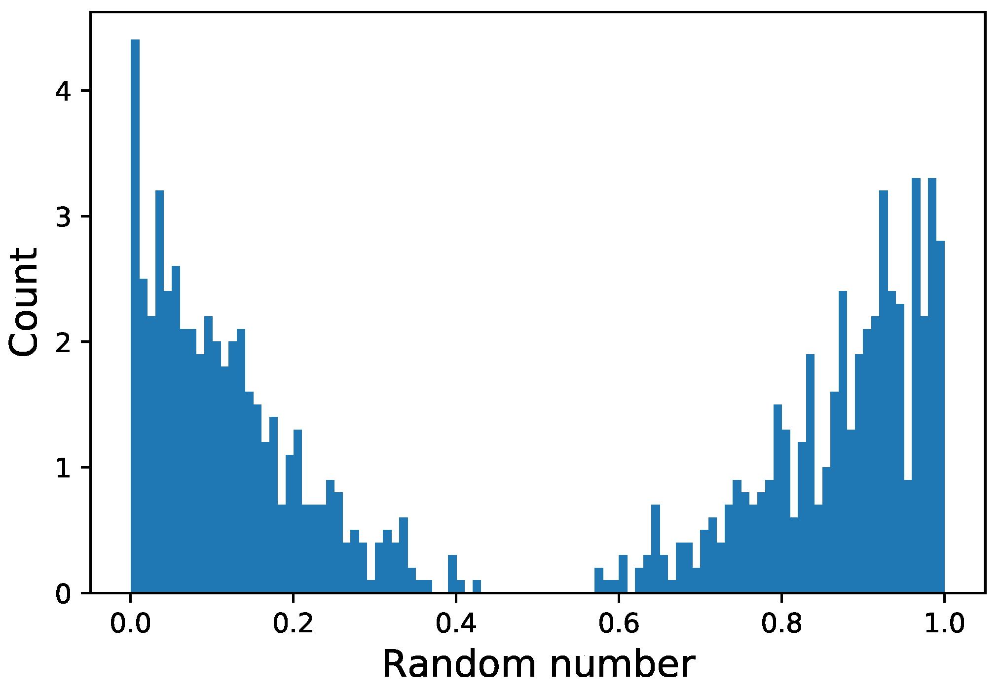
We propose extended version of SMOTE to generate the final synthetic portfolio, X s , as described in Section 2.1. Extended SMOTE is primarily different from the original SMOTE in just a single step: the interpolation step. The detailed procedure is the following: for each feature vector (observation, x i r ), the distance between x i r and the other feature vectors in X r is computed based on the Euclidean distance to obtain 5 nearest neighbors for each x i r . Subsequently, one x i r and corresponding one-nearest neighbor are randomly selected. The difference between x i r and this neighbor is multiplied by a random number drawn from the U-shape distribution, as shown in Figure 2. Adding the random number to the x i r , we create a synthetic feature vector, x i s . 100,000 synthetic observations are generated, which consisted of the synthetic portfolio, X s . After applying the extended SMOTE, the following considerations had also been reflected in the synthetic portfolio generation:
  • integer features are rounded up;
  • for categorical features, only Car.use are multi-class. Car.use is converted by one-hot coding before applying extended SMOTE so that every categorical feature variable has the value 0 or 1. After the generation, they are rounded up; and,
  • for compositional features, Pct.drive.sun and Pct.drive.wkend are not involved in the generation process, but are calculated by ‘1 − the rest of related features.’

4.1.2. The Simulation of Number of Claims

To mimic the real telematics data, the next step is to build the simulation generating Y 1 s , with four categorical values. It is a multi-class classification problem. However, we converted it into multiple binary class classifications to make each process simple and simultaneously improve the accuracy of simulation. In each simulation function, x is input and z is output, where z 11 ( 1 ) r indicates the Z 1 r value corresponding to x 1 ( 1 ) r .
  • Sub-simulation 1: Z 1 r = 𝟙 Y 1 r 1 . Corresponding instance index is
    { 1 ( 1 ) , 2 ( 1 ) , , M ( 1 ) } . The data is given as the following:
    D 1 = { ( x 1 ( 1 ) r , z 11 ( 1 ) r ) , ( x 2 ( 1 ) r , z 12 ( 1 ) r ) , , ( x M ( 1 ) r , z 1 M ( 1 ) r ) }
  • Sub-simulation 2: Z 2 r = 𝟙 Y 1 r 2 | Y 1 r 1 . Corresponding instance index is
    { 1 ( 2 ) , 2 ( 2 ) , , M ( 2 ) } . The data is given as the following:
    D 2 = { ( x 1 ( 2 ) r , z 21 ( 2 ) r ) , ( x 2 ( 2 ) r , z 2 2 ( 2 ) r ) , , ( x M ( 2 ) r , z 2 M ( 2 ) r ) }
  • Sub-simulation 3: Z 3 r = 𝟙 Y 1 r = 3 | Y 1 r 2 . Corresponding instance index is
    { 1 ( 3 ) , 2 ( 3 ) , , M ( 3 ) } . The data is given as the following:
    D 3 = { ( x 1 ( 3 ) r , z 31 ( 3 ) r ) , ( x 2 ( 3 ) r , z 3 2 ( 3 ) r ) , , ( x M ( 3 ) r , z 3 M ( 3 ) r ) }
The feedforward neural network simulation is learned from each D k . Hyperparameters are tuned via Gaussian Process (GP) algorithm, as detailed in the previous section: the number of hidden layers, the number of nodes for first hidden layer, the number of nodes for the rest of the hidden layers, activation functions, batch size, and the learning rate. Table 5 introduces the resultant architecture of the network. We set up sigmoid activation function for output layer, since this is a binary problem; it has the value between 0 and 1. Threshold is 0.5 and cross entropy loss function is used. The weight of the neural network is optimized using the Adam optimizer. In the Adam optimizer, as input values, we need α ( learning rate ) , β 1 , β 2 , and ϵ . See Algorithm 1 of Kingma and Ba (2014). In practice, β 1 = 0.9 , β 2 = 0.999 , and ϵ = 1 e 08 are commonly used, and no further tuning is usually done. Thus, we only tuned the learning rate via GP.
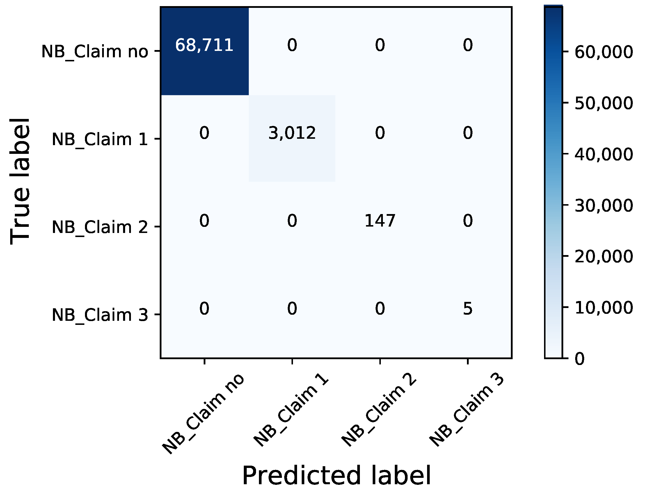
Figure 3 shows the accuracy of the three sub-simulations. When the real portfolio is plugged in, its prediction reveals 100% coincidence with the real number of claims. This implies that as we plug in realistic portfolio into this combined frequency simulation, we are able to arrive at realistic number of claims.
After building three sub-simulations, plugging in synthetically generated portfolio, X s into sub-simulation 1, we get Z 1 s . Subsequently, we extract X s | Z 1 s = 1 , plugging it into sub-simulation 2 and get the value, Z 2 s . Likewise, plugging in X s | Z 2 s = 1 into sub-simulation 3, we obtain the final one, Z 3 s . By combining these three results, we finally generate synthetic number of claims, Y 1 s .

4.1.3. The Simulation of Aggregated Amount of Claims

We produce the subset of portfolios, which satisfies the condition, Y 1 r > 0 . Corresponding to a new index of the subset is defined as { 1 ( s e v ) , 2 ( s e v ) , , M ( s e v ) } . The number and amount of claims are not treated independent to each other, but, rather, the number of claims Y 1 r , is also considered as one of the feature variables. Therefore, we use the following data to train the aggregated amount of claims simulation:
D 4 = { ( ( x 1 ( s e v ) r , y 11 ( s e v ) r ) , y 21 ( s e v ) r ) , ( ( x 2 ( s e v ) r , y 12 ( s e v ) r ) , y 22 ( s e v ) r ) , , ( ( x M ( s e v ) r , y 1 M ( s e v ) r ) , y 2 M ( s e v ) r ) }
Y 2 r is a non-negative continuous value. Thus, in the second simulation, we use ReLU as the activation function and MSE as the loss function. Adam optimizers are used with the hyperparameters that are selected in the same manner, as described in Section 4.1.2. These are further described in Table 6.
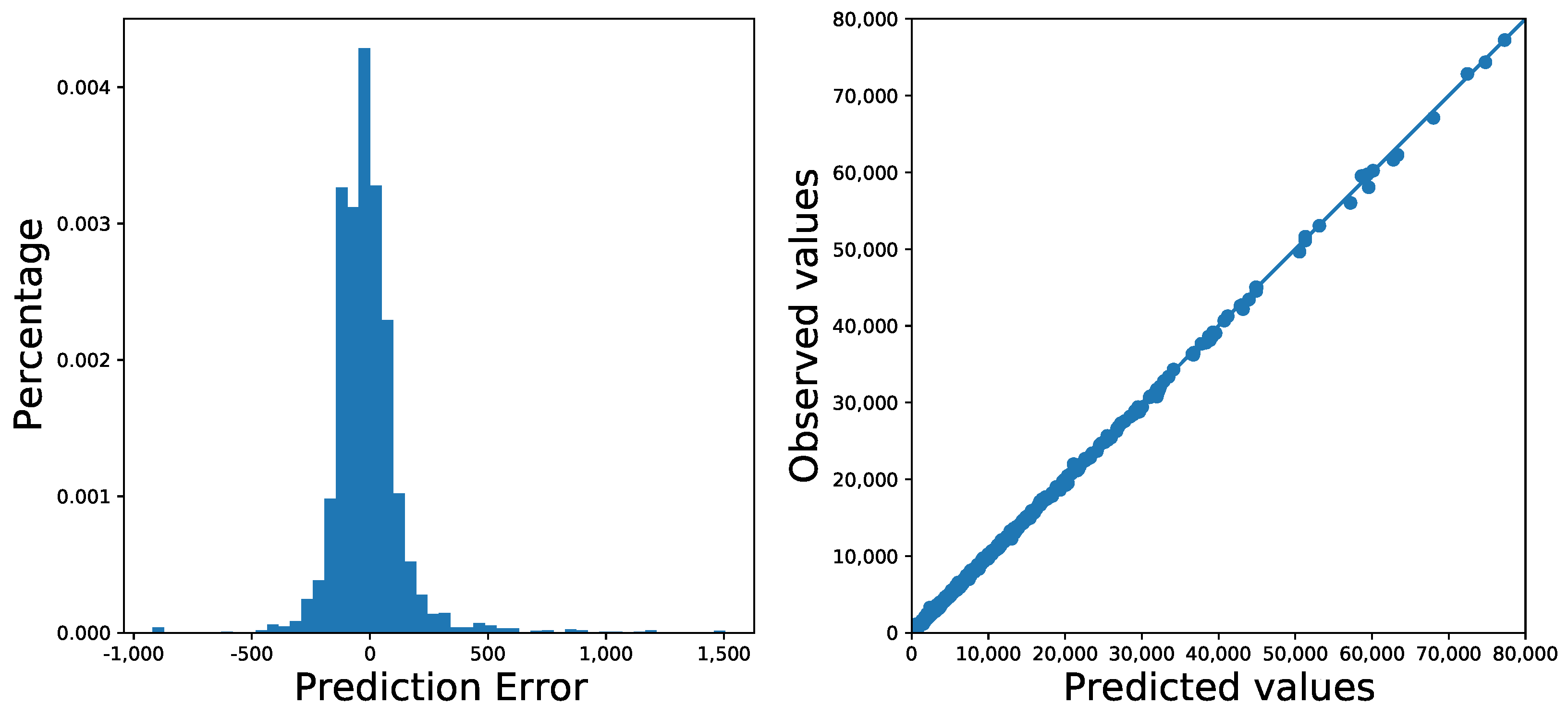
Figure 4 reveals the resulting performance of the claims simulation. The prediction errors are highly centered around zero and most of the dots are on the line of QQ plot for predicted and real claim amount. This sufficiently proves that the simulation can imitate the real amount of claim with a synthetic portfolio based on the number of claims simulation introduced in Section 4.1.2.
To generate Y 2 s , we use Y 1 s obtained from Section 4.1.2, and we extract the subset of synthetic portfolio with the condition, Y 1 s > 0 . This subset of synthetic portfolio and corresponding Y 1 s are the input of the simulation to obtain Y 2 s .

4.2. Comparison: Poisson and Gamma Regression

Combining every output ( X s , Y 1 s , Y 2 s ) obtained from Section 4.1, the data with telematics features are thereby complete. Any statistical or machine learning algorithms can now be performed on this completed synthetic datafile. In order to frther compare the quality of the reconstruction of the real dataset to produce the synthetic datafile, one simple approach is to compare the resulting outputs when a Poisson regression model is calibrated on the number of claims (frequency) and a gamma regression model is calibrated on the amount of claims (severity), while using the respective real dataset and the synthetic datafile. Both of the models are relatively standard benchmark models in practice. To be more specific, we fitted both Poisson and gamma regression models to the real and synthetic data to predict the number of claims ( NB _ Claim Duration ) and the average amount of claims ( AMT _ Claim NB _ Claim | NB _ Claim > 0 ). A net premium can be calculated by taking the product of the number of claims and the average amount of claims. The purpose of this exercise is not to evaluate the quality of the models or the relative importance of the feature variables, but rather to compare the resulting outputs between the two datasets. The training models are based on all of the feature variables in the absence of variable selection.
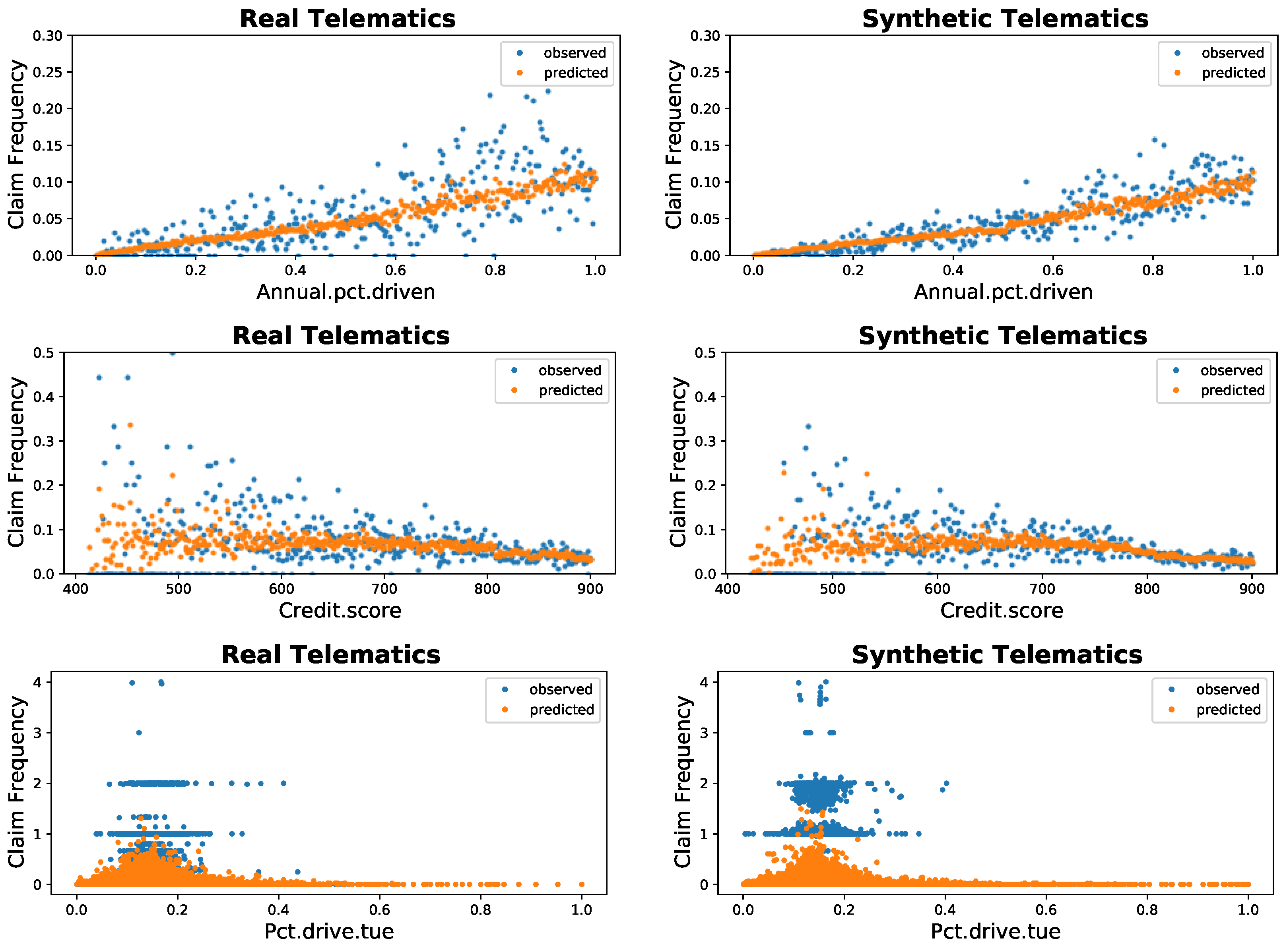
Figure 5 describes the average claim frequency between the real telematics on the left side and the synthetic telematics on the right side. For simplicity, we only provide the behavior of the claim frequency for three feature variables: Annual.pct.drive, Credit.score, and Pct.drive.tue. For both of the datasets, we see that the observed values are colored blue and the predicted values are colored orange. As we expected, the distributions of the average claim frequency, as well as the pattern of blue and orange, for these feature variables considered here have very similar patterns between the real and synthetic datasets.
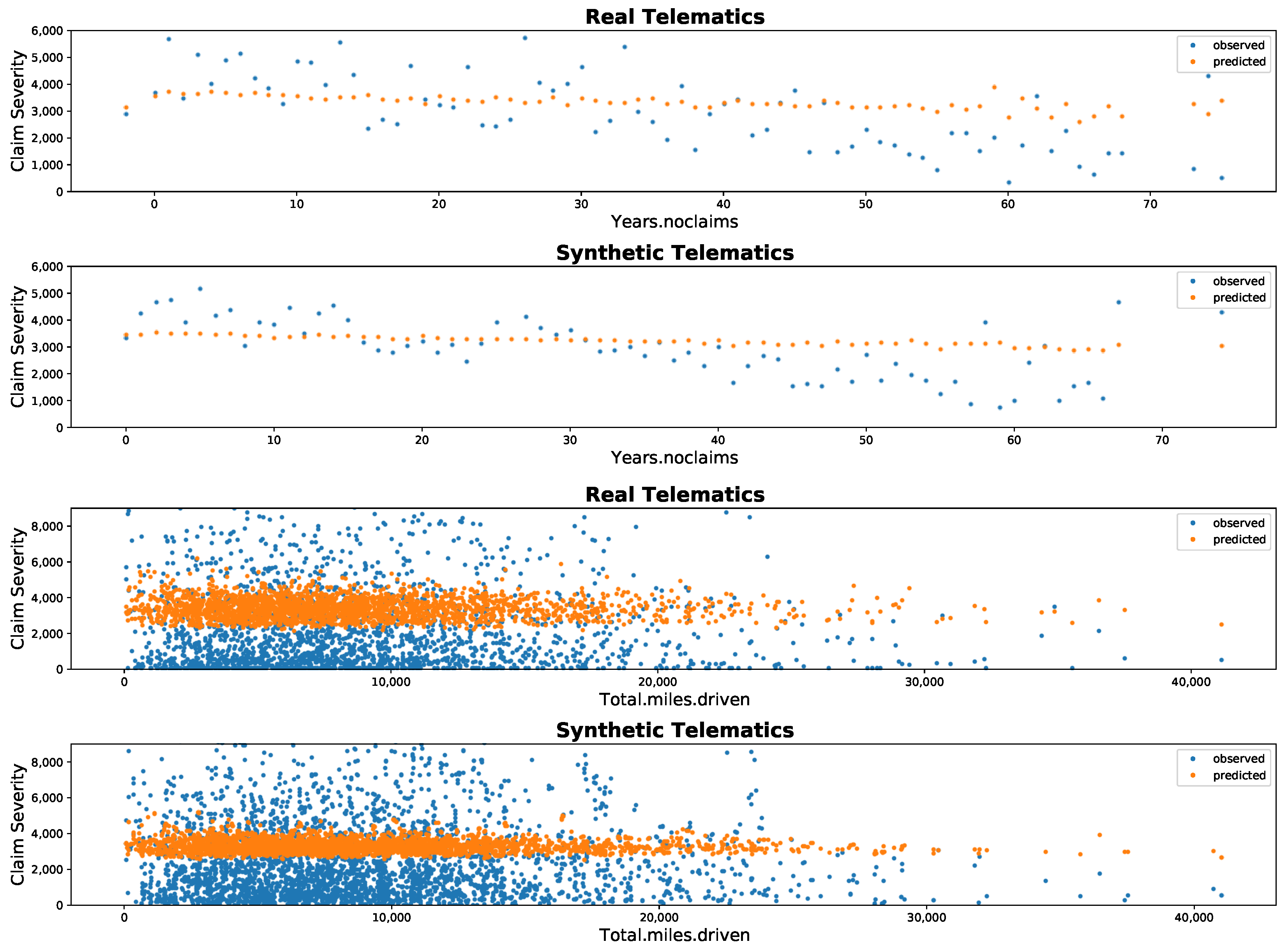
As similarly done for frequency, Figure 6 depicts the average claim severity between the real telematics and the synthetic telematics. For our purpose, we examine these comparisons based on two feature variables: Yrs.noclaims and Total.miles.driven. Both of these feature variables do not seem to produce much variation in the predicted values: this may explain that these are relatively less important predictor variables for claims severity. However, this may also be explained by the fact that we do not necessarily have an exceptionally good model here for prediction. However, this is not the purpose of this exercise.
Still, from both Figure 5 and Figure 6, there is some information we can draw. First, the patterns of blue dots are similar between the real and synthetic data for every feature variable considered here. Even though we do not include the graphs of other features, for all features they show similar dispersion. The included features are the one considered as important variables based on the classification models introduced in So et al. (2020). This seems to suggest that real and synthetic data have similar frequency and feature distributions for all variables, which implies that the synthetic datafile is behaving as realistic as the real data. In conclusion, it mimics the real dataset exceptionally well. Second, the patterns of orange dots are also similar between the real and synthetic data. In more details, predicted frequency (Figure 5) and severity (Figure 6) from models tuned based on real data have a similar dispersion with those from the model tuned on synthetic data. This suggests results obtained by synthetic data might have little difference from the results obtained by real data, and, conclusively, we can use synthetic data to train statistical models in place of real data.
Figure 7 further supports these conclusions, which shows a quantile–quantile (QQ) plot of the predicted pure premium between the real data and the synthetic data. We do, however, observe that we tend to overestimate the pure premium for the synthetic datafile for high quantiles. This may be a result of the randomness produced throughout the data generation process. This is not, by any means, an alarming concern.

5. Concluding Remarks

It has been discussed that there is a perceived positive social effect to vehicle telematics: it encourages careful driving behavior. Indeed, UBI programs can have many potential benefits to insurers, consumers, and society, in general. Insurers are permitted to put a price tag that links information that is more directly related to habits of insured drivers. As a consequence, this helps insurance companies to provide customers the opportunity for more affordable premiums and to increase the predictability of their profit margin. On the other hand, consumers may be able to control the level of premium costs by maintaining safer driving habits or if at all possible, by reducing the frequency of driving. Furthermore, UBI may benefit the society, because, with safer driving and fewer drivers on the road, this may reduce the frequency of accidents, traffic congestion, and car emissions. In order to get the optimal benefits of UBI to both insurers and their policyholders, it becomes subsequently crucial to identify the more significant telematics variables that truly affect the occurrence of car accidents. These perceived positive benefits motivated us to provide the research community a synthetic datafile, which has the intricacies and characteristics of a real data, that may be used to examine, construct, build, and test better predictive models that can immediately be put into practice. For additional details of benefits of UBI, see Husnjak et al. (2015).
In summary, this paper describes the generating process used to produce a synthetic datafile of driver telematics that has largely been based and emulated from a similar real insurance dataset. The final synthetic dataset produced has 100,000 policies that included observations regarding driver’s claims experience, together with associated classical risk variables and telematics-related variables. One primary motivation for such production is to encourage the research community to develop innovative and more powerful predictive models; this synthetic datafile can be used to train and test such predictive models so that we can provide better techniques that can be used in practice to assess UBI products. As alluded throughout this paper, the data generation is best described as a three-stage process of applying extended SMOTE algorithm to produce synthetic portfolio of feature variables and using feedforward neural networks to simulate the number and aggregated amount of claims. The resulting data generation is evaluated by a comparison between the synthetic data and real data when Poisson and gamma regression models are fitted to the respective data. Data summarization and visualization of these resulting fitted models between the two datasets produce remarkably similar statistics and patterns. Additional figures provided in Appendix A suggest the notable similarities between the two datasets. We are hopeful that researchers that are interested in obtaining driver telematics datasets to calibrate statistical models or machine learning algorithms will find the output of this research helpful for their purpose. We encourage the research community to build better predictive models and test these models with our synthetic datafile.

Author Contributions

Conceptualization, B.S., J.-P.B. and E.A.V.; methodology, B.S., J.-P.B. and E.A.V.; software, B.S., J.-P.B. and E.A.V.; validation, B.S., J.-P.B. and E.A.V.; formal analysis, B.S., J.-P.B. and E.A.V.; investigation, B.S., J.-P.B. and E.A.V.; resources, B.S., J.-P.B. and E.A.V.; data curation, B.S., J.-P.B. and E.A.V.; writing—original draft preparation, B.S., J.-P.B. and E.A.V.; writing—review and editing, B.S., J.-P.B. and E.A.V.; visualization, B.S., J.-P.B. and E.A.V.; supervision, E.A.V.; project administration, E.A.V.; funding acquisition, E.A.V. All authors have read and agreed to the published version of the manuscript.

Funding

This research has been funded by the Society of Actuaries through its Centers of Actuarial Excellence (CAE) grant for our project on “Applying Data Mining Techniques in Actuarial Science”.

Institutional Review Board Statement

Not applicable.

Informed Consent Statement

Not applicable.

Data Availability Statement

Proprietary data has been used in the analysis and may not be shared.

Acknowledgments

The authors want to thank The Co-operators General Insurance Company for providing the data. Banghee So acknowledges and thanks the support from the Society of Actuaries through its James C. Hickman Scholar program. The authors thank the referees and editor for their comments and suggestions which helped improve the final version of this work.

Conflicts of Interest

The authors declare no conflict of interest.

Appendix A. Graphical Display of Distributions of Selected Variables between Synthetic and Real Datasets

The figures in this appendix provide summarization and visualization of selected variables in the datasets. These figures provide suggestions of how remarkably similar the distributions of the two datasets, an indication how good our procedure generated the synthetic datasets. Note that we can only provide distribution summaries in order to preserve confidentiality of the original data used in the generation. The figures are self-explanatory.
Figure A1. Synthetic data: Distribution of average number of claims for six telematics-related features.
Risks 09 00058 g0a1
Figure A2. Real data: Distribution of average number of claims for six telematics-related features.
Risks 09 00058 g0a2
Figure A3. Synthetic data: Distribution of average number of claims for four traditional features.
Risks 09 00058 g0a3
Figure A4. Real data: Distribution of average number of claims for four traditional features.
Risks 09 00058 g0a4

References

  1. Arik, Sercan O., Markus Kliegl, Rewon Child, Joel Hestness, Andrew Gibiansky, Chris Fougner, Ryan Prenger, and Adam Coates. 2017. Convolutional recurrent neural networks for small-footprint keyword spotting. arXiv arXiv:1703.05390. [Google Scholar]
  2. Ayuso, Mercedes, Montserrat Guillen, and Jens P. Nielsen. 2019. Improving automobile insurance ratemaking using telematics: Incorporating mileage and driver behaviour data. Transportation 46: 735–52. [Google Scholar] [CrossRef] [Green Version]
  3. Ayuso, Mercedes, Montserrat Guillén, and Ana María Pérez-Marín. 2014. Time and distance to first accident and driving patterns of young drivers with pay-as-you-drive insurance. Accident Analysis and Prevention 73: 125–31. [Google Scholar] [CrossRef] [PubMed]
  4. Ayuso, Mercedes, Montserrat Guillen, and Ana María Pérez-Marín. 2016. Telematics and gender discrimination: Some usage-based evidence on whether men’s risk of accidents differs from women’s. Risks 4: 10. [Google Scholar] [CrossRef] [Green Version]
  5. Baecke, Philippe, and Lorenzo Bocca. 2017. The value of vehicle telematics data in insurance risk selection processes. Decision Support Systems 98: 69–79. [Google Scholar] [CrossRef]
  6. Bansal, Trapit, David Belanger, and Andrew McCallum. 2016. Ask the GRU: Multi-task learning for deep text recommendations. arXiv arXiv:1609.02116v2. [Google Scholar]
  7. Bergstra, James, and Yoshua Bengio. 2012. Random search for hyper-parameter optimization. Journal of Machine Learning Research 13: 281–305. [Google Scholar]
  8. Bergstra, James S., Rémi Bardenet, Yoshua Bengio, Balázs Kégl, James S. Bergstra, Rémi Bardenet, Yoshua Bengio, and Balázs Kégl. 2011. Algorithms for hyper-parameter optimization. In Advances in Neural Information Processing Systems. New York: Curan Associates Inc., pp. 2546–54. [Google Scholar]
  9. Boucher, Jean-Philippe, Steven Côté, and Montserrat Guillen. 2017. Exposure as duration and distance in telematics motor insurance using generalized additive models. Risks 5: 54. [Google Scholar] [CrossRef] [Green Version]
  10. Butler, Patrick. 1993. Cost-based pricing of individual automobile risk transfer: Car-mile exposure unit analysis. Journal of Actuarial Practice 1: 51–67. [Google Scholar]
  11. Chawla, Nitesh V., Kevin W. Bowyer, Lawrence O. Hall, and W. Philip Kegelmeyer. 2002. SMOTE: Synthetic Minority Over-sampling Technique. Journal of Artificial Intelligence Research 16: 321–57. [Google Scholar] [CrossRef]
  12. Dalkilic, Turkan Erbay, Fatih Tank, and Kamile Sanli Kula. 2009. Neural networks approach for determining total claim amounts in insurance. Insurance: Mathematics and Economics 45: 236–41. [Google Scholar] [CrossRef]
  13. Denuit, Michel, Xavier Maréchal, Sandra Piterbois, and Jean-François Walhin. 2007. Actuarial Modelling of Claim Counts: Risk Classification, Credibility and Bonus-Malus Systems. West Sussex: John Wiley & Sons. [Google Scholar]
  14. Duchi, John, Elad Hazan, and Yoram Singer. 2011. Adaptive subgradient methods for online learning and stochastic optimization. Journal of Machine Learning Research 12: 2121–59. [Google Scholar]
  15. Fernández, Alberto, Salvador Garcia, Francisco Herrera, and Nitesh V. Chawla. 2018. SMOTE for learning from imbalanced data: Progress and challenges, marking the 15-year anniversary. Journal of Artificial Intelligence Research 61: 863–905. [Google Scholar] [CrossRef]
  16. Franceschi, Luca, Michele Donini, Paolo Frasconi, and Massimiliano Pontil. 2017. Forward and reverse gradient-based hyperparameter optimization. Paper presented at 34th International Conference on Machine Learning, Sydney, Australia, August 6–11; pp. 1165–73. [Google Scholar]
  17. Gabrielli, Andrea, and Mario V. Wüthrich. 2018. An individual claims history simulation machine. Risks 6: 29. [Google Scholar] [CrossRef] [Green Version]
  18. Gan, Guojun, and Emiliano A. Valdez. 2007. Valuation of large variable annuity portfolios: Monte Carlo simulation and synthetic datasets. Dependence Modeling 5: 354–74. [Google Scholar] [CrossRef]
  19. Gan, Guojun, and Emiliano A. Valdez. 2018. Nested stochastic valuation of large variable annuity portfolios: Monte Carlo simulation and synthetic datasets. Data 3: 1–21. [Google Scholar]
  20. Gao, Guangyuan, Shengwang Meng, and Mario V. Wüthrich. 2019. Claim frequency modeling using telematics car driving data. Scandinavian Actuarial Journal 2: 143–62. [Google Scholar] [CrossRef]
  21. Goodfellow, Ian, Yoshua Bengio, and Aaron Courville. 2016. Deep Learning. Cambridge, MA: MIT Press. [Google Scholar]
  22. Guillen, Montserrat, Jens P. Nielsen, Ana María Pérez-Marín, and Valandis Elpidorou. 2020. Can automobile insurance telematics predict the risk of near-miss events? North American Actuarial Journal 24: 141–52. [Google Scholar] [CrossRef] [Green Version]
  23. Guillen, Montserrat, Jens P. Nielsen, Mercedes Ayuso, and Ana M. Pérez-Marín. 2019. The use of telematics devices to improve automobile insurance rates. Risk Analysis 39: 662–72. [Google Scholar] [CrossRef]
  24. Hornik, Kurt, Maxwell Stinchcombe, and Halbert White. 1989. Multilayer feedforward networks are universal approximators. Neural Networks 2: 359–66. [Google Scholar] [CrossRef]
  25. Husnjak, Siniša, Dragan Peraković, Ivan Forenbacher, and Marijan Mumdziev. 2015. Telmatics system in usage based motor insurance. Procedia Engineering 100: 816–25. [Google Scholar] [CrossRef] [Green Version]
  26. Ibiwoye, Ade, Olawale O. E. Ajibola, and Ashim B. Sogunro. 2012. Artificial neural network model for predicting insurance insolvency. International Journal of Management and Business Research 2: 59–68. [Google Scholar]
  27. Karapiperis, Dimitris, Birny Birnbaum, Aaron Bradenburg, Sandra Catagna, Allen Greenberg, Robin Harbage, and Anne Obersteadt. 2015. Usage-Based Insurance and Vehicle Telematics: Insurance Market and Regulatory Implications. Technical Report. Kansas City: National Association of Insurance Commissioners and The Center for Insurance Policy and Research. [Google Scholar]
  28. Kiermayer, Mark, and Christian Weiß. 2020. Grouping of contracts in insurance using neural networks. Scandinavian Actuarial Journal, 1–28. [Google Scholar] [CrossRef]
  29. Kingma, Diederik P., and Jimmy Ba. 2014. Adam: A method for stochastic optimization. arXiv arXiv:1412.6980. [Google Scholar]
  30. Li, Jing, Ji-Hang Cheng, Jing-Yuan Shi, and Fei Huang. 2012. Brief introduction of back propagation (BP) neural network algorithm and its improvement. Advances in Intelligent and Soft Computing 169: 553–58. [Google Scholar]
  31. Maclaurin, Dougal, David Duvenaud, and Ryan Adams. 2015. Gradient-based hyperparameter optimization through reversible learning. Paper presented at 32nd International Conference on Machine Learning, Lille, France, July 6–11; Volume 37, pp. 2113–22. [Google Scholar]
  32. McCulloch, Warren S., and Walter Pitts. 1943. A logical calculus of the ideas immanent in nervous activity. The Bulletin of Mathematical Biophysics 5: 115–33. [Google Scholar] [CrossRef]
  33. Murugan, Pushparaja. 2017. Hyperparameters optimization in deep convolutional neural network/bayesian approach with gaussian process prior. arXiv arXiv:1712.07233. [Google Scholar]
  34. Osafune, Tatsuaki, Toshimitsu Takahashi, Noboru Kiyama, Tsuneo Sobue, Hirozumi Yamaguchi, and Teruo Higashino. 2017. Analysis of accident risks from driving behaviors. International Journal of Intelligent Transportation Systems Research 15: 192–202. [Google Scholar] [CrossRef]
  35. Peng, Yifan, Anthony Rios, Ramakanth Kavuluru, and Zhiyong Lu. 2018. Chemical-protein relation extraction with ensembles of svm, cnn, and rnn models. arXiv arXiv:1802.01255. [Google Scholar]
  36. Pesantez-Narvaez, Jessica, Montserrat Guillen, and Manuela Alcañiz. 2019. Predicting motor insurance claims using telematics data—XGBoost versus logistic regression. Risks 7: 70. [Google Scholar] [CrossRef] [Green Version]
  37. Pérez-Marín, Ana M., Montserrat Guillen, Manuela Alcañiz, and Lluís Bermúdez. 2019. Quantile regression with telematics information to assess the risk of driving above the posted speed limit. Risks 7: 80. [Google Scholar] [CrossRef] [Green Version]
  38. Ruder, Sebastian. 2016. An overview of gradient descent optimization algorithms. arXiv arXiv:1609.04747. [Google Scholar]
  39. Snoek, Jasper, Hugo Larochelle, and Ryan P. Adams. 2012. Practical Bayesian optimization of machine learning algorithms. In Advances in Neural Information Processing Systems. New York: Curan Associates Inc., pp. 2951–59. [Google Scholar]
  40. So, Banghee, Jean-Philippe Boucher, and Emiliano A. Valdez. 2020. Cost-sensitive multi-class adaboost for understanding driving behavior with telematics. arXiv arXiv:2007.03100. [Google Scholar] [CrossRef]
  41. Thiede, Luca Anthony, and Ulrich Parlitz. 2019. Gradient based hyperparameter optimization in echo state networks. Neural Networks 115: 23–29. [Google Scholar] [CrossRef]
  42. Verbelen, Roel, Katrien Antonio, and Gerda Claeskens. 2018. Unravelling the predictive power of telematics data in car insurance pricing. Journal of the Royal Statistical Society: Series C Applied Statistics 67: 1275–304. [Google Scholar] [CrossRef] [Green Version]
  43. Viaene, Stijn, Guido Dedene, and Richard A. Derrig. 2005. Auto claim fraud detection using Bayesian learning neural networks. Expert Systems with Applications 29: 653–66. [Google Scholar] [CrossRef]
  44. Wüthrich, Mario V. 2019. Bias regularization in neural network models for general insurance pricing. European Actuarial Journal 10: 179–202. [Google Scholar] [CrossRef]
  45. Yan, Chun, Meixuan Li, Wei Liu, and Man Qi. 2020. Improved adaptive genetic algorithm for the vehicle insurance fraud identification model based on a bp neural network. Theoretical Computer Science 817: 12–23. [Google Scholar] [CrossRef]
  46. Zhang, Jingzhao, SaiPraneeth Karimireddy, Andreas Veit, Seungyeon Kim, SashankJ Reddi, Sanjiv Kumar, and Suvrit Sra. 2019. Why Adam beats SGD for attention models. arXiv arXiv:1912.03194. [Google Scholar]
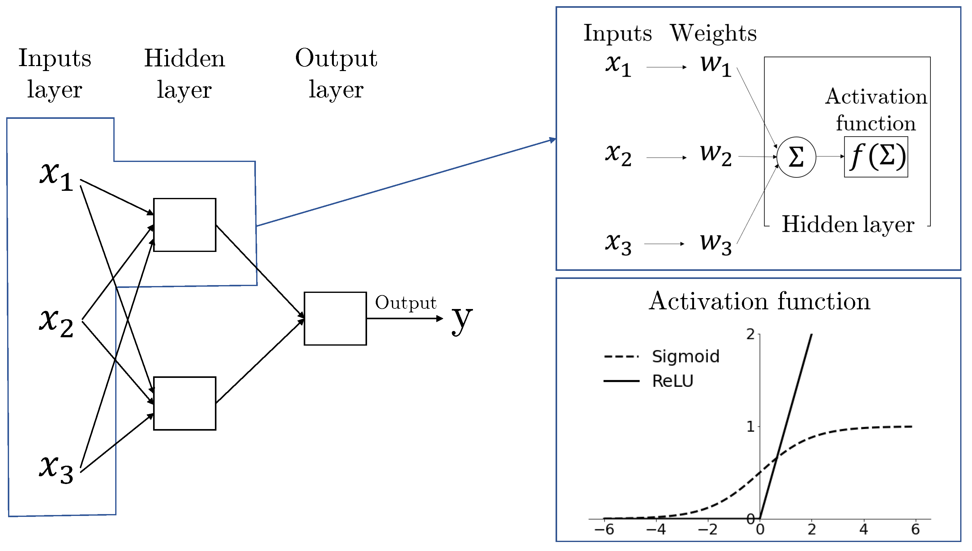
Figure 1. Architecture of a feedforward neural network.
Risks 09 00058 g001
Figure 2. 1000 random numbers drawn from the U-shape distribution.
Risks 09 00058 g002
Figure 3. Confusion matrix based on the number of claims simulation results.
Risks 09 00058 g003
Figure 4. Assessing the accuracy of the simulation of aggregated amount of claims.
Risks 09 00058 g004
Figure 5. Average claim frequency using real (left) and synthetic (right) datasets.
Risks 09 00058 g005
Figure 6. Average severity using real (1st & 3rd) and synthetic (2nd & 4th) datasets.
Risks 09 00058 g006
Figure 7. QQ-plot of predicted pure premium: real and synthetic data.
Risks 09 00058 g007
Table 1. An overview of the literature.
Data SourceReferenceSamplePeriodAnalytical TechniquesResearch Synthesis
BelgiumVerbelen et al. (2018)10,406 drivers
(33,259 obs.)
2010–2014Poisson GAM,
Negative binomial GAM
Shows that the presence of telematics variables are better important predictors of driving habits
CanadaSo et al. (2020)71,875 obs.2013–2016Adaboost,
SAMME.C2
Demonstrates telematics information improves the accuracy of claims frequency prediction with a new boosting algorithm
ChinaGao et al. (2019)1478 drivers2014.01–2017.06Poisson GAMShows the relevance of telematics covariates extracted from speed-acceleration heatmaps in a claim frequency model
EuropeBaecke and Bocca (2017)6984 drivers
(<age 30)
2011–2015Logistic regression,
Random forests,
Neural networks
Illustrates the importance of telematics variables for pricing UBI products and shows that as few as three months of data may already be enough to obtain efficient risk estimates
GreeceGuillen et al. (2020)157 drivers
(1225 obs.)
2016– 2017Negative binomial reg.Demonstrates how the information drawn from telematics can help predict near-miss events
JapanOsafune et al. (2017)809 drivers2013.12–2015.02Support Vector MachinesInvestigates accident risk indices that statistically separate safe and risky drivers
SpainAyuso et al. (2014)15,940 drivers
(<age 30)
2009–2011Weibull regressionCompares driving behaviors of novice and experienced young drivers with PAYD policies
Ayuso et al. (2016)8198 drivers
(<age 30)
2009–2011Weibull regressionDetermines the use of gender becomes irrelevant in the presence of sufficient telematics information
Boucher et al. (2017)71,489 obs.2011Poisson GAMOffers the benefits of using generalized additive models (GAM) to gain additional insights as to how premiums can be more dynamically assessed with telematics information
Guillen et al. (2019)25,014 drivers
(<age 40)
2011Zero-inflated PoissonInvestigates how telematics information helps explain part of the occurrence of zero accidents not typically accounted by traditional risk factors
Ayuso et al. (2019)25,014 drivers
(<age 40)
2011Poisson regressionIncorporates information drawn from telematics metrics into classical frequency model for tariff determination
Pérez-Marín et al. (2019)9614 drivers
(<age 35)
2010Quantile regressionDemonstrates that the use of quantile regression allows for better identification of factors associated with risky drivers
Pesantez-Narvaez et al. (2019)2767 drivers
(<age 30)
2011XGBoostExamines and compares the performance of XGBoost algorithm against the traditional logistic regression
Table 2. Variable names and descriptions.
TypeVariableDescription
TraditionalDurationDuration of the insurance coverage of a given policy, in days
Insured.ageAge of insured driver, in years
Insured.sexSex of insured driver (Male/Female)
Car.ageAge of vehicle, in years
MaritalMarital status (Single/Married)
Car.useUse of vehicle: Private, Commute, Farmer, Commercial
Credit.scoreCredit score of insured driver
RegionType of region where driver lives: rural, urban
Annual.miles.driveAnnual miles expected to be driven declared by driver
Years.noclaimsNumber of years without any claims
TerritoryTerritorial location of vehicle
TelematicsAnnual.pct.drivenAnnualized percentage of time on the road
Total.miles.drivenTotal distance driven in miles
Pct.drive.xxxPercent of driving day xxx of the week: mon/tue/…/sun
Pct.drive.xhrsPercent vehicle driven within x hrs: 2hrs/3hrs/4hrs
Pct.drive.xxxPercent vehicle driven during xxx: wkday/wkend
Pct.drive.rushxxPercent of driving during xx rush hours: am/pm
Avgdays.weekMean number of days used per week
Accel.xxmilesNumber of sudden acceleration 6/8/9/…/14 mph/s per 1000 miles
Brake.xxmilesNumber of sudden brakes 6/8/9/…/14 mph/s per 1000 miles
Left.turn.intensityxxNumber of left turn per 1000 miles with intensity 08/09/10/11/12
Right.turn.intensityxxNumber of right turn per 1000 miles with intensity 08/09/10/11/12
ResponseNB_ClaimNumber of claims during observation
AMT_ClaimAggregated amount of claims during observation
Table 3. Summary statistics of AMT_Claim based on synthetic NB_Claim: Synthetic vs. Real.
SyntheticNB_ClaimMeanStd DevMinQ1MedianQ3Max
AMT_Claim00000000
140626767067021914776138,767
28960955402350703411,22556,780
35437231428963620537256989743
RealNB_ClaimMeanStd DevMinQ1MedianQ3Max
AMT_Claim00000000
146468387065922385140145,153
2864310,92001739518411,08262,259
35682207932534540541657739521
Table 4. Data types of all the 52 variables in the synthetic dataset.
CategoryContinuous/IntegerPercentageCompositional
MaritalDurationAnnual.pct.drivenPct.drive.mon
Insured.sexInsured.agePct.drive.xhrsPct.drive.tue
Car.useCar.agePct.drive.rushxx       .
RegionCredit.score        .
TerritoryAnnual.miles.drive Pct.drive.sun
NB_ClaimYears.noclaims Pct.drive.wkday
Total.miles.driven Pct.drive.wkend
Avgdays.week
Accel.xxmiles
Brake.xxmiles
Left.turn.intensityxx
Right.turn.intensityxx
AMT_Claim
Table 5. The architecture of the three sub-simulations for number of claims.
ArchitectureN.Hidden L.N.Nodes_First Hidden L.N.Nodes_Rest Hidden L.ActivationBatchSizeLearning R.
sub-sim1335368ReLU850.000667
sub-sim2347367ReLU180.001019
sub-sim326060ReLU160.001922
Table 6. The architecture of simulation for the aggregated amount of claims.
ArchitectureN.Hidden L.N.Nodes_First Hidden L.N.Nodes_Rest Hidden L.ActivationBatchSizeLearning R.
634467ReLU30.000526
Publisher’s Note: MDPI stays neutral with regard to jurisdictional claims in published maps and institutional affiliations.