Article

Concordance Probability for Insurance Pricing Models

1
Department of Mathematics, Katholieke Universiteit Leuven, 3000 Leuven, Belgium
2
Data Office, Allianz Benelux, 1000 Brussels, Belgium
3
Department of Mathematics, University of Antwerp, 2020 Antwerp, Belgium
*
Author to whom correspondence should be addressed.
Risks 2021, 9(10), 178; https://doi.org/10.3390/risks9100178
Submission received: 18 August 2021 / Revised: 24 September 2021 / Accepted: 29 September 2021 / Published: 8 October 2021
(This article belongs to the Special Issue Data Mining in Actuarial Science: Theory and Applications)

Abstract

:
The concordance probability, also called the C-index, is a popular measure to capture the discriminatory ability of a predictive model. In this article, the definition of this measure is adapted to the specific needs of the frequency and severity model, typically used during the technical pricing of a non-life insurance product. For the frequency model, the need of two different groups is tackled by defining three new types of the concordance probability. Secondly, these adapted definitions deal with the concept of exposure, which is the duration of a policy or insurance contract. Frequency data typically have a large sample size and therefore we present two fast and accurate estimation procedures for big data. Their good performance is illustrated on two real-life datasets. Upon these examples, we also estimate the concordance probability developed for severity models.

1. Introduction

One of the main tasks of an insurer is to determine the expected number of claims that will be received for a certain line of business and how much the average claim will cost. The former is typically predicted using a frequency model, whereas the latter is obtained by a severity model. The multiplication of these expected values then yields the technical premium (for more information, we refer to Frees (2009); Ohlsson and Johansson (2010)). Alternatively, one can also model the frequency and severity jointly (Shi et al. 2015). Predictive analytics are a key tool to develop both frequency and severity model in a data-driven way. Note that insurers also use a variety of predictive analytic tools in many other applications such as underwriting, marketing, fraud detection and claims reserving (Frees et al. 2014, 2016; Wuthrich and Buser 2020). The main goal of predictive analytics is typically to capture the predictive ability of the model of interest. Important aspects of the predictive ability of a model are the calibration and the discriminatory ability. Calibration expresses how close the predictions are to the actual outcome, while discrimination quantifies how well the predictions separate the higher risk observations from the lower risk observations (Steyerberg et al. 2010). Even though both calibration and discrimination are of utmost importance when constructing predictive models in general, the discrimination probably is considered to be slightly more important in the context of non-life insurance pricing. The technical premium should first and foremost capture the difference in risk that is present in the portfolio, which is exactly captured by discriminatory measures. The concordance probability typically is the most popular and widely used measure to gauge the discriminatory ability of a predictive model.
In case we have a discrete response variable Y, it equals the probability that a randomly selected subject with outcome Y = 0 has a lower predicted probability than a randomly selected subject with outcome Y = 1 (Pencina and D’Agostino 2004). Here, π ( X ) equals P ( Y = 1 | X ) , with X corresponding to the vector of predictors. In other words, the concordance probability C can be formulated as:   
C = P π ( X i ) > π ( X j ) | Y i = 1 , Y j = 0 .
Furthermore, in a discrete setting and in the absence of ties in the predictions, this concordance probability equals the Area Under the ROC Curve (AUC) (Reddy and Aggarwal 2015). This ROC curve is the Receiver Operating Characteristic curve, suggested by Bamber (1975). It represents the true positive rate against the false positive rate at several threshold settings. The AUC is a popular performance measure to check the discriminatory ability of a binary classifier, as can be seen in the work of Liu et al. (2008) for example.
Even if definition (1) looks very promising to assess the discriminatory ability of frequency models, it assumes that the outcome variable is a binary rather than a count random variable. Moreover, since the policy runtime or exposure of an insurance contract typically is included as an offset variable in the frequency model, definition (1) needs to be extended to accommodate the presence of such an offset variable.
When dealing with a continuous outcome Y, this basic definition is typically adapted as:
C = P π ( X i ) > π ( X j ) | Y i > Y j .
We say that the pairs π ( X i ) , Y i and π ( X j ) , Y j are concordant when sgn( π ( X i ) π ( X j ) ) = sgn( Y i Y j ). Hence, the probability that a randomly selected comparable pair of observations with their predictions is a concordant pair, is another way of formulating the definition of the concordance probability. Note that definition (2) is a very popular measure in the field of survival analysis, where the continuous outcome corresponds to the time-to-event variable (Legrand 2021). For the severity model, it can be argued whether it is important to discriminate claims for which the observed cost hardly differs, hence an extension of definition (2) will be considered. Since the estimation of any definition of the concordance probability is time-consuming for larger datasets, we will also consider time-efficient and accurate estimation procedures.
In this paper, we will focus on the concordance probability applied to frequency and severity models used to construct a technical premium P for an insurance contract. This technical premium typically corresponds to the product of the expected probability of occurrence of the event ( E ( Y N ) ) times the expected cost of the event ( E ( Y S ) ). Note that these expectations are often conditional on some variables, such that the technical premium corresponds to
P = E Y N | X N × E Y S | X S ,
with X N and X S the set of variables that are used to model each random variable. From here on, ( Y N , X N ) will be referred to as the frequency data and ( Y S , X S ) to as the severity data.
First, we introduce in Section 2 the real datasets that will be used throughout this article, together with the frequency and severity models based on them. Section 3 covers the required changes of the general concordance probabilities (1) and (2), such that they can be applied in an insurance context. Next, we develop several algorithms that calculate these new definitions in an accurate and time-efficient way. These algorithms will be introduced in Section 4, where they are immediately applied to the introduced models. Finally, the conclusion is given in Section 5.

2. Datasets and Models

In this section, we first introduce some real datasets. Next, we explain the frequency and severity models using these datasets.

2.1. Datasets

The datasets explained in this section, are all obtained from the pricing games of the French Institute of Actuaries, which is a game that can be played by both students and practitioners. First, we discuss the one of the 2015 pricing game and next we consider the ones of the 2016 pricing game. Both datasets are publicly available in the R-package CASdatasets1 and contain data on which both a frequency and severity model can be applied.

2.1.1. 2015 Pricing Game

The pg15training dataset was used for the 2015 pricing game of the French Institute of Actuaries organized on 5 November 2015 and contains 100,021 third-party liability (TPL) policies for private motor insurance. Each observation pertains to a different policy and a set of variables has been collected of the policyholder and the insured vehicle.
For reasons of confidentiality, most categorical levels have an unknown meaning. This dataset can be used for the frequency and severity model, and the selected and renamed variables are explained in Appendix A. The two most important ones are claimNumb and claimCharge, which will be the dependent variables of the frequency and severity analysis respectively. The variable claimNumb shows the number of third-party bodily injury claims. For policies for which more than two claims were filed during the considered exposure, the value was set to 2. This adaptation is needed for the measures that are presented in Section 3. The variable claimCharge represents the total cost of third-party bodily injury claims, in euro. Finally, exposure will be used as an offset variable during the analysis of the frequency data. It is the percentage of a full policy year, corresponding to the run time of the respective policy. Note that 72.58 % of the observations have an exposure equal to one.

2.1.2. 2016 Pricing Game

pg16trainpol and pg16trainclaim are two datasets that were used for the same pricing game of the French Institute of Actuaries one year later, in 2016. Both of them can be found in the R -package CASdatasets. The first dataset contains 87,226 policies for private motor insurance and can be used for the frequency model. The pg16trainclaim dataset contains 4568 claims of those 87,226 TPL policies and combined with the pg16trainpol dataset, the severity model can be constructed. Policies are guaranteed for all kinds of material damages, but not bodily injuries.
Once again, most categorical levels have an unknown meaning for reasons of confidentiality. The selected and renamed variables of the pg16trainpol and pg16trainclaim dataset are explained in Appendix A. The two most important ones are claimNumb and claimCharge, which will be the dependent variables of the frequency and severity analysis respectively. The variable claimNumb shows the number of claims. The policies for which more than two claims were filed during the considered exposure, the value was once again set to 2. This adaptation is needed for the measures that are presented in Section 3. The variable claimCharge represent the claim size. Moreover, exposure will be used as an offset variable during the analysis of the frequency data. It is the percentage of a full policy year, corresponding to the run time of the respective policy. In this dataset, 14.16% of the observations have an exposure equal to one.
Note that we only selected the 3969 observations that had a strictly positive claim, to construct the severity model. Finally, we could merge the pg16trainclaim and the pg16trainpol datasets based on the their policy number, begin date, end date and license number.

2.2. Models

In this subsection, we construct the frequency and severity models based on the aforementioned datasets. It is important to know that the interest of this paper is not really on the construction of the models, but on the calculation of the concordance probability of the models once the predictions are available. For both models, we first split the required dataset in a training and a test set. The training set is obtained by selecting 60% of the observations of the entire dataset. The remaining 40% of the observations represent the test set.

2.2.1. Frequency

In order to obtain predictions of the frequency model, we consider a basic Poisson model where the variable claimNumb is the response variable. The exposure is used as an offset variable, and all other variables of the training set, apart from claimCharge, are considered as predictor variables. Applying the frequency model on the test set of the 2015 (2016) pricing game, we obtain 40,008 (34,890) pairs of observations and their corresponding predictions. However, the goal of this paper is to calculate the concordance probability of these frequency models for big datasets. Therefore, we will also consider a bootstrap of these pairs of observations and predictions, resulting in 1,000,000 pairs for each dataset.

2.2.2. Severity

In order to obtain predictions for the severity, we consider a gamma model where the ratio of claimCharge over claimNumb is the response variable, and the weights are equal to the variable claimNumb. This is a popular approach for severity models, as explained in Appendix B, based on the book of Denuit et al. (2007). All other variables of the training set, apart from exposure and claimNumb, are considered as predictors. Applying the severity model on the test set of the 2015 (2016) pricing game, we obtain 1837 (1588) pairs of observations and their corresponding predictions. However, the goal of this paper is to calculate the concordance probability of these severity models for big datasets. Therefore, we will also consider a bootstrap of these pairs of observations and predictions, resulting in 1,000,000 pairs for each dataset.

3. Concordance Probability in an Insurance Setting

In this section, the general definitions (1) and (2) of the concordance probability will be modified to the use for frequency and severity models.

3.1. Frequency Models

The general definition of the concordance probability will in this section be modified to a concordance probability that can be used for frequency models. The basic definition (1) requires the definition of two groups, based on the number of events that occurred during the duration of the policy. However, non-life insurance contracts typically have an exposure of maximum one year. Hence, it is unlikely that more than two events will take place during this (short) period. Therefore, three groups will be defined: policies that experienced zero events, one event, and two events or more, respectively represented by the 0-, 1- and 2-group. These groups result in the following three definitions of the concordance probability for frequency models:
C 0 , 1 + = P π N ( X i ) < π N ( X j ) | Y i N = 0 , Y j N 1 , C 0 , 2 + = P π N ( X i ) < π N ( X j ) | Y i N = 0 , Y j N 2 , C 1 , 2 + = P π N ( X i ) < π N ( X j ) | Y i N = 1 , Y j N 2 ,
where π N ( · ) refers to the predicted frequency of the frequency model and Y N to the observed claim number. The set of definitions (3) has several interesting interpretations. First of all, C 0 , 1 + ( C 0 , 2 + ) evaluates the ability of the model to discriminate policies that did not encounter accidents from policies that encountered at least one (two) accident(s). Furthermore, C 1 , 2 + quantifies the ability of the model to discriminate policies that encountered one accident from policies that encountered multiple accidents. In other words, C 1 , 2 + quantifies the ability of the model to discriminate clients that could just have been unfortunate versus clients that are (probably) accident-prone.
However, these concordance probabilities do not take the concept of exposure into account. This is the duration of a policy or insurance contract, and plays a pivotal role in frequency models. In order to make sure that the pair is comparable, the definition of the concordance probability needs to be extended to deal with the concept of exposure as well. As such, two main possibilities can be imagined which ensures comparability of the given pair. For the first possibility, the member of the pair that experienced the most accidents needs to have an exposure that is equal to or lower than the exposure of the other member of the pair. These pairs are sort of comparable since the member of the pair that experienced the most accidents did not have a longer policy duration than the member of the pair that experienced the fewest accidents. The set of definitions (3) can then be altered as:
C 0 , 1 + λ = P π N ( X i ) < π N ( X j ) | Y i N = 0 , Y j N 1 , λ i λ j , C 0 , 2 + λ = P π N ( X i ) < π N ( X j ) | Y i N = 0 , Y j N 2 , λ i λ j , C 1 , 2 + λ = P π N ( X i ) < π N ( X j ) | Y i N = 1 , Y j N 2 , λ i λ j ,
where λ i corresponds to the exposure of observation i. However, the above set of definitions (4) runs into trouble for pairs where there is a considerable difference in exposure. In order to understand why this is the case, we need to have a look at the structure of the predictions of a Poisson regression model, which corresponds for observation i to π N ( X i ) = λ i exp ( β X i ) . This reveals that the prediction is mainly determined by the exposure λ i and the linear predictor β X i . Therefore, when the predictions of a Poisson regression model of a pair of observations are compared, two possibilities can occur when the pair is comparable according to the above set of definitions (4). One member of the pair can have a higher prediction than the other member due to a difference in risk, as expressed by the linear predictor and as is desirable, or due to a mere difference in exposure, which would obscure the analysis. A possible solution would be to set the exposure values of all observations equal to 1 when making predictions, such that one only focuses on the difference in risk between the different observations. However, this is undesirable as we would like to evaluate the predictions of the Poisson model that are used to compute the expected cost of the insurance policy, and for this the exposure is a key ingredient. In other words, the set of definitions (4) are of little practical use within the domain of insurance and will no longer be considered.
For the second possibility, the exposure λ of both members of the pair need to be more or less the same, in order to ensure their comparability. Incorporated in the set of definitions (3), we get:
C 0 , 1 + ( γ ) = P π N ( X i ) < π N ( X j ) | Y i N = 0 , Y j N 1 , | λ i λ j | γ , C 0 , 2 + ( γ ) = P π N ( X i ) < π N ( X j ) | Y i N = 0 , Y j N 2 , | λ i λ j | γ , C 1 , 2 + ( γ ) = P π N ( X i ) < π N ( X j ) | Y i N = 1 , Y j N 2 , | λ i λ j | γ .
Here, γ is a tuning parameter representing the maximal difference in exposure between both members of a pair that is considered to be negligible.
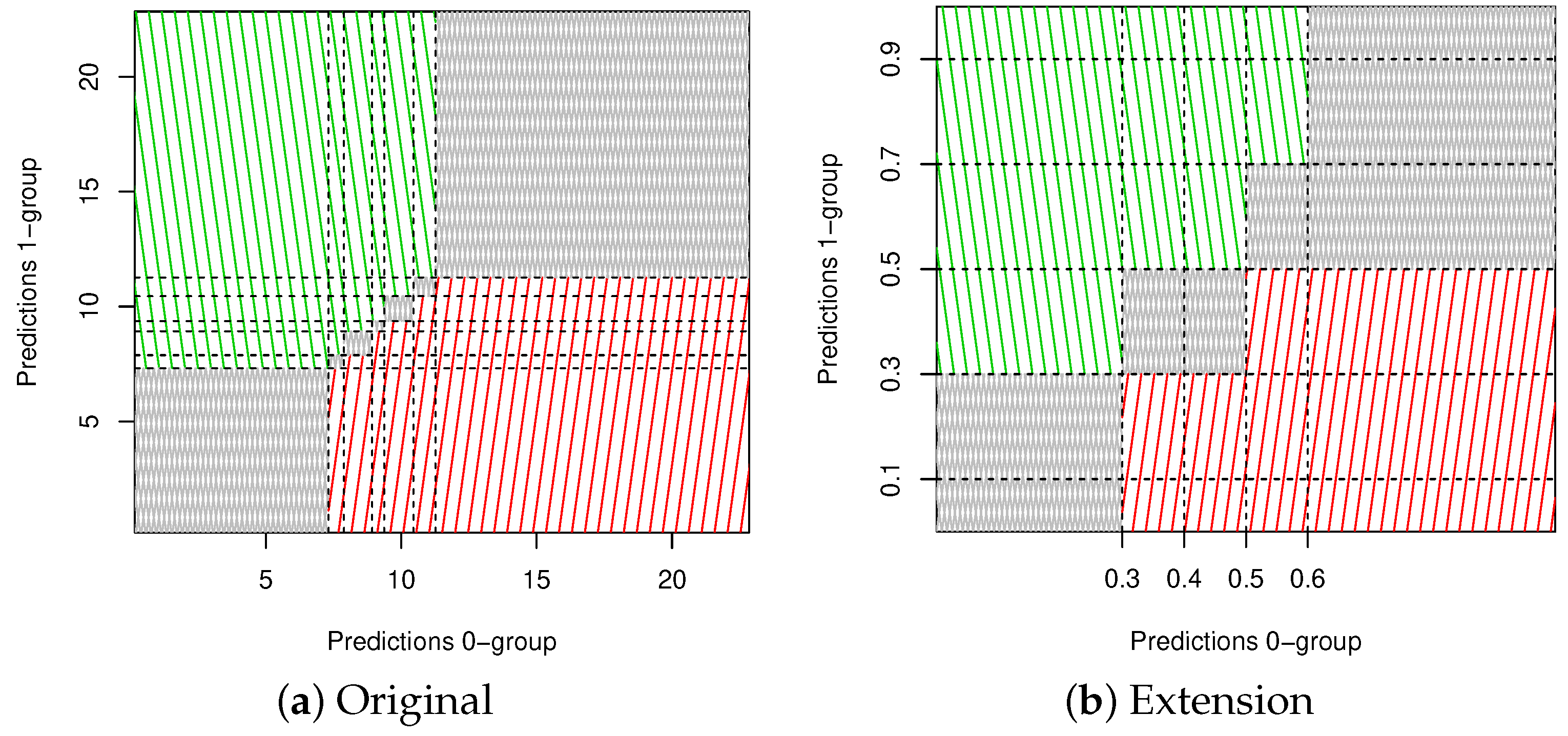
All former definitions are global measures, meaning that the concordance probability is computed over all observations of the dataset, where comparability is considered as the sole exclusion criterion for a given pair. The following definitions show a local concordance probability, by taking a subset of the complete dataset based on the exposure:
C 0 , 1 + ( λ , γ ) = P π N ( X i ) < π N ( X j ) | Y i N = 0 , Y j N 1 , { λ i , λ j } [ λ ± γ / 2 ] , C 0 , 2 + ( λ , γ ) = P π N ( X i ) < π N ( X j ) | Y i N = 0 , Y j N 2 , { λ i , λ j } [ λ ± γ / 2 ] , C 1 , 2 + ( λ , γ ) = P π N ( X i ) < π N ( X j ) | Y i N = 1 , Y j N 2 , { λ i , λ j } [ λ ± γ / 2 ] .
In the above set of definitions, λ is the parameter corresponding to the exposure value for which the local concordance probability needs to be computed. In practice, C . , . . + ( γ ) C . , . . + ( 1 , γ ) because the main mass of the data is located at a full exposure. The appealing aspect of this set of definitions is that it allows the construction of a ( λ , C ( λ , γ ) ) table, i.e., an evolution of the local concordance probabilities in function of the exposure. However, the disadvantage of this plot is that one has to choose the values of λ and γ . Assume one takes γ equal to 0.05 and λ { 0.05 , 0.15 , , 0.95 } . In this case, observations with for example exposure 0.49 and 0.51 will not be comparable, although their exposures are very close to each other. To eliminate this issue, we first define two groups:
  • O -group: group with the largest number of elements, hence the group with the smallest number of events,
  • 1 -group: group with the smallest number of elements, hence the group containing the largest number of events.
When we consider for example C 1 , 2 + ( λ , γ ) , the O -group consists of the elements with Y N = 1 and the 1 -group of the elements with Y N 2 . Next, we apply following steps to construct a better ( λ , C ( λ , γ ) ) plot:
  • Determine the pairs of observations and predictions belonging to the O -group and the ones to the 1 -group.
  • Define the number of unique exposures λ within 1 and apply a for-loop on them:
    • Select the elements in 1 with exposure λ i .
    • Select the elements in O with exposure in [ max ( 0 , λ i γ ) , min ( 1 , λ i + γ ) ] .
    • Determine C ( λ i , γ ) , the concordance probability on these two subsets.
    • Define m i , the number of comparable pairs used to calculate C ( λ i , γ ) .
  • The global concordance probability C ( γ ) can be rewritten as:
    C ( γ ) = i = 1 n 1 j = i + 1 n I π ^ ( x i ) > π ^ ( x j ) , y i 1 , y j O , | λ j λ i | < γ i = 1 n 1 j = i + 1 n I π ^ ( x i ) π ^ ( x j ) , y i 1 , y j O , | λ j λ i | < γ = i = 1 n 1 j = 1 n 0 I π ^ ( x i ) > π ^ ( x j ) , | λ j λ i | < γ i = 1 n 1 j = 1 n 0 I π ^ ( x i ) π ^ ( x j ) , | λ j λ i | < γ = i = 1 n 1 m i C ( λ i , γ ) i = 1 n 1 m i = i w i C ( λ i , γ ) ,
    where n equals the number of observations, n 0 ( n 1 ) the number of observations in O ( 1 ), n 1 the number of unique exposures in 1 and w i = m i i = 1 n 1 m i .
  • Construct the plot of C ( λ i , γ ) in function of λ i .
Since the loop iterates over all unique exposures in the 1 -group, which is the smallest one, the x-axis can have a rather rough grid. Therefore, one can also easily adapt the previous steps by looping over the unique exposures in the O -group, resulting in a plot with an 
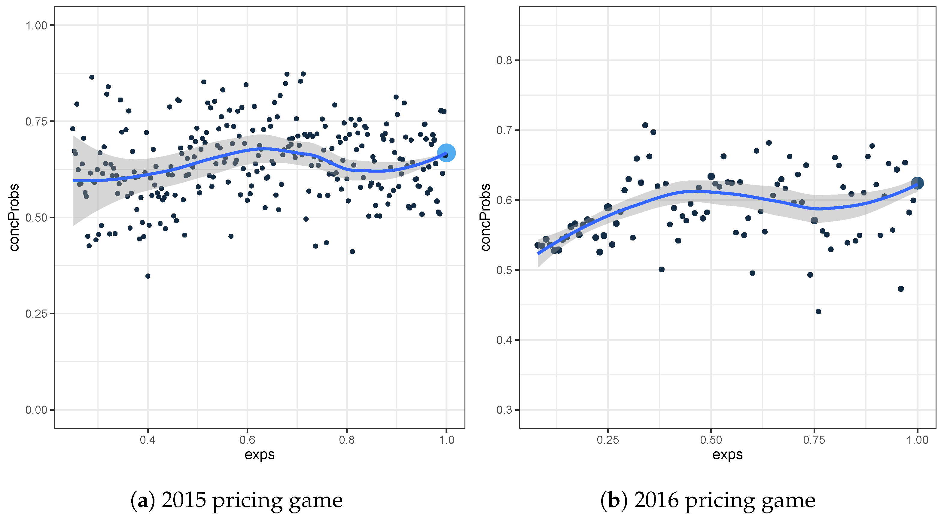
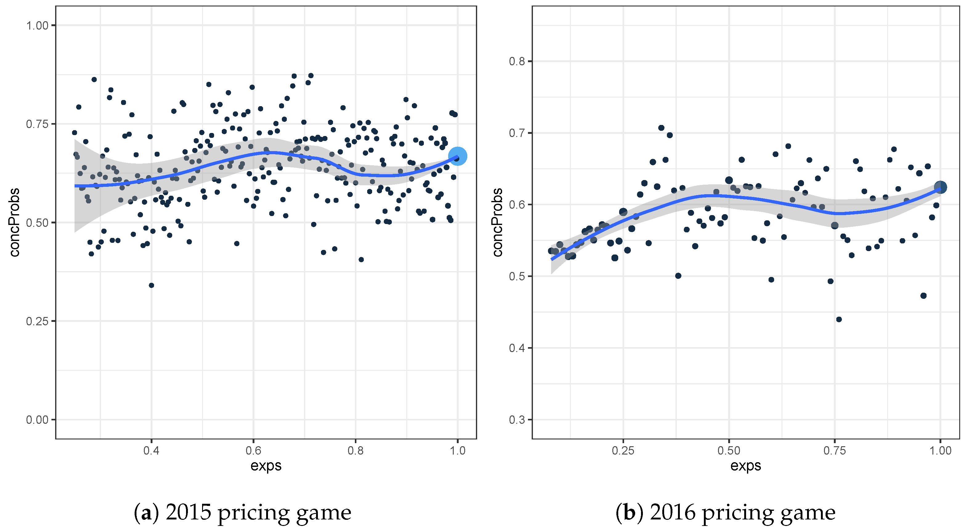
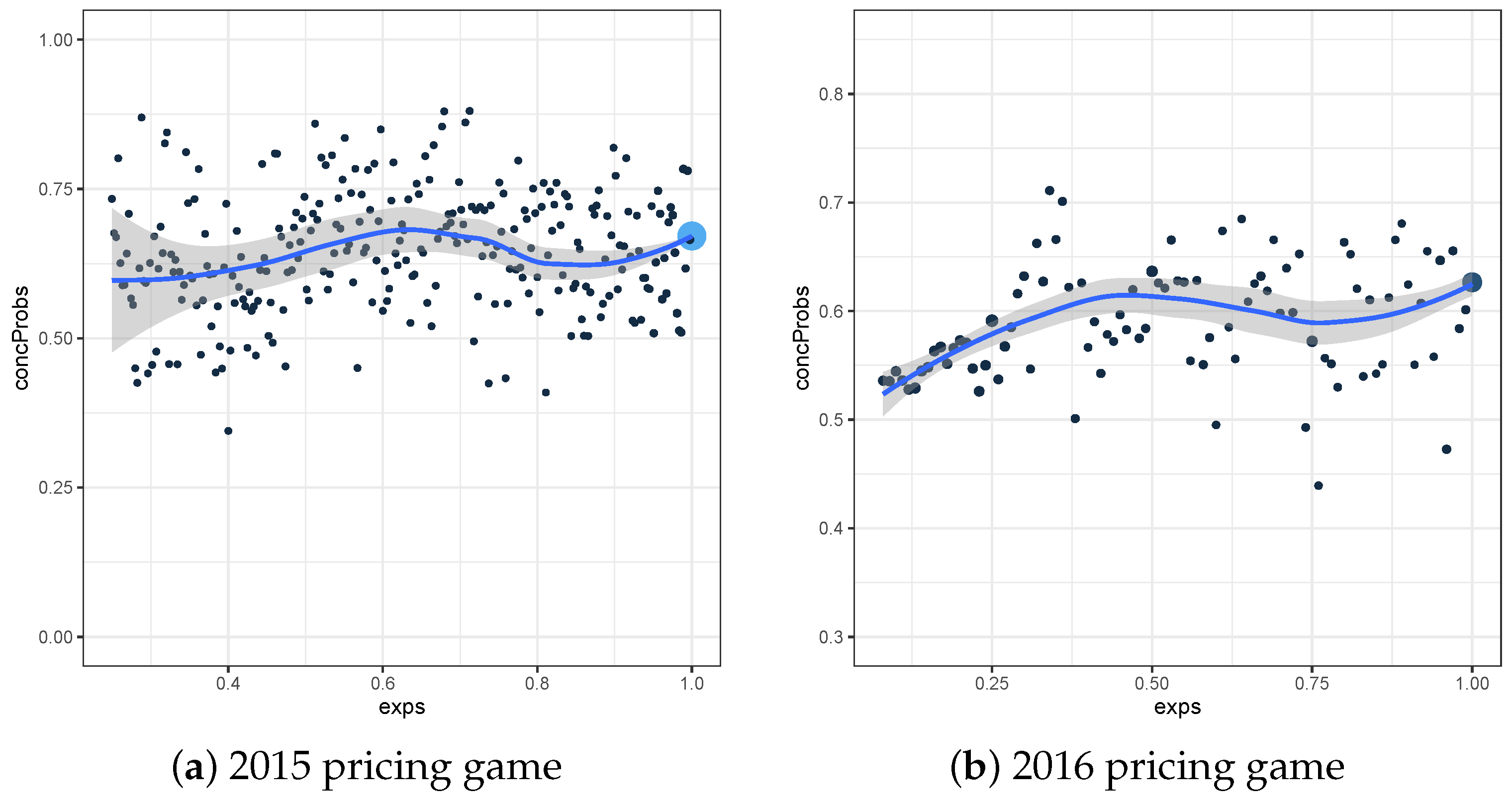
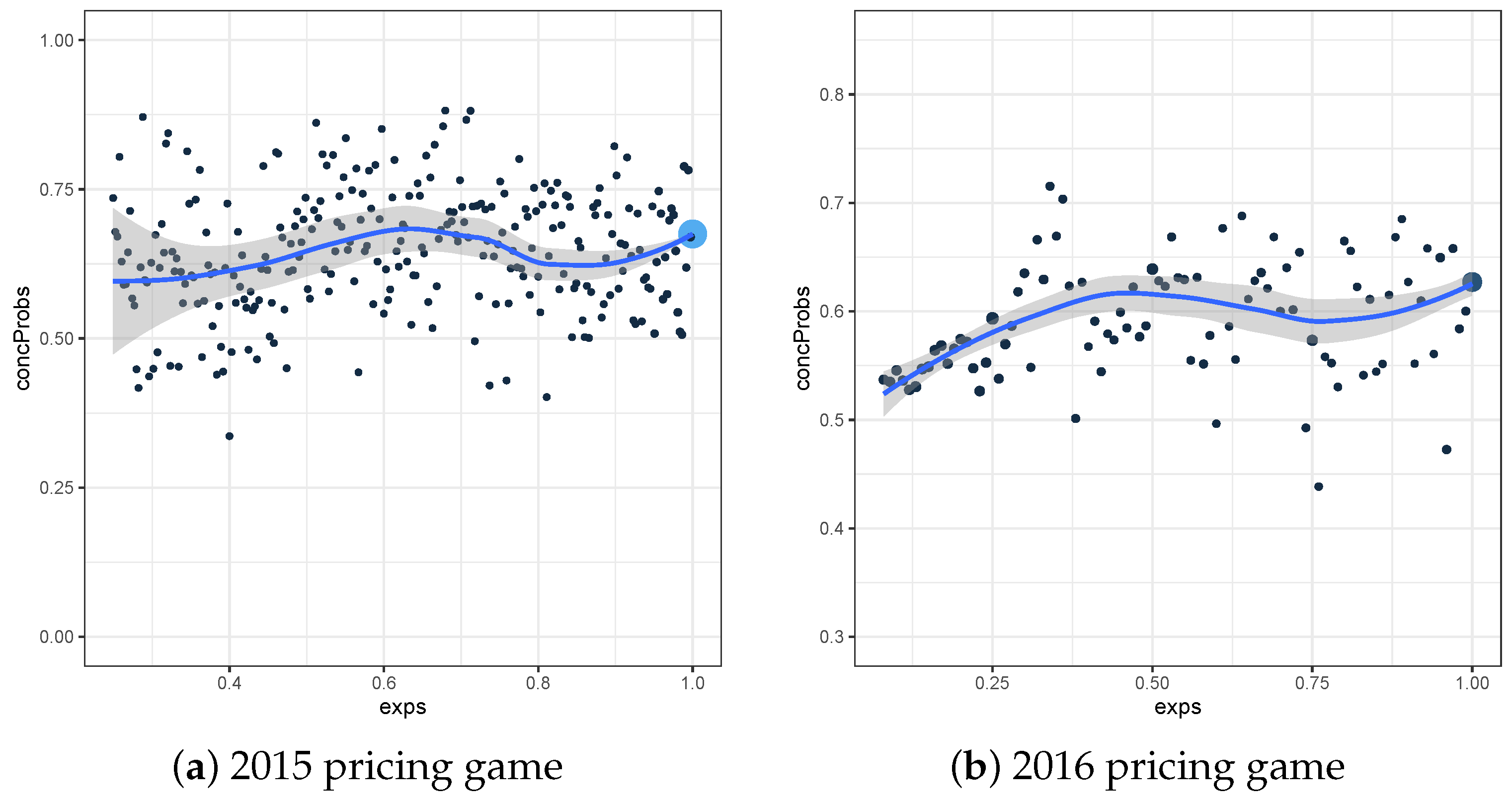
x-axis that has possibly a finer grid. In Figure 1 and Figure 2, both the rough and the fine version of the ( λ , C 0 , 1 + ( λ , γ ) ) plot are constructed for the test sets of the 2015 and 2016 pricing game respectively. We choose γ to be 0.05, which is approximately equal to the length of one month. For the test set of the 2015 (2016) pricing game, the maximal weight w i is 0.96 (0.32) for the observations with exposure 1.
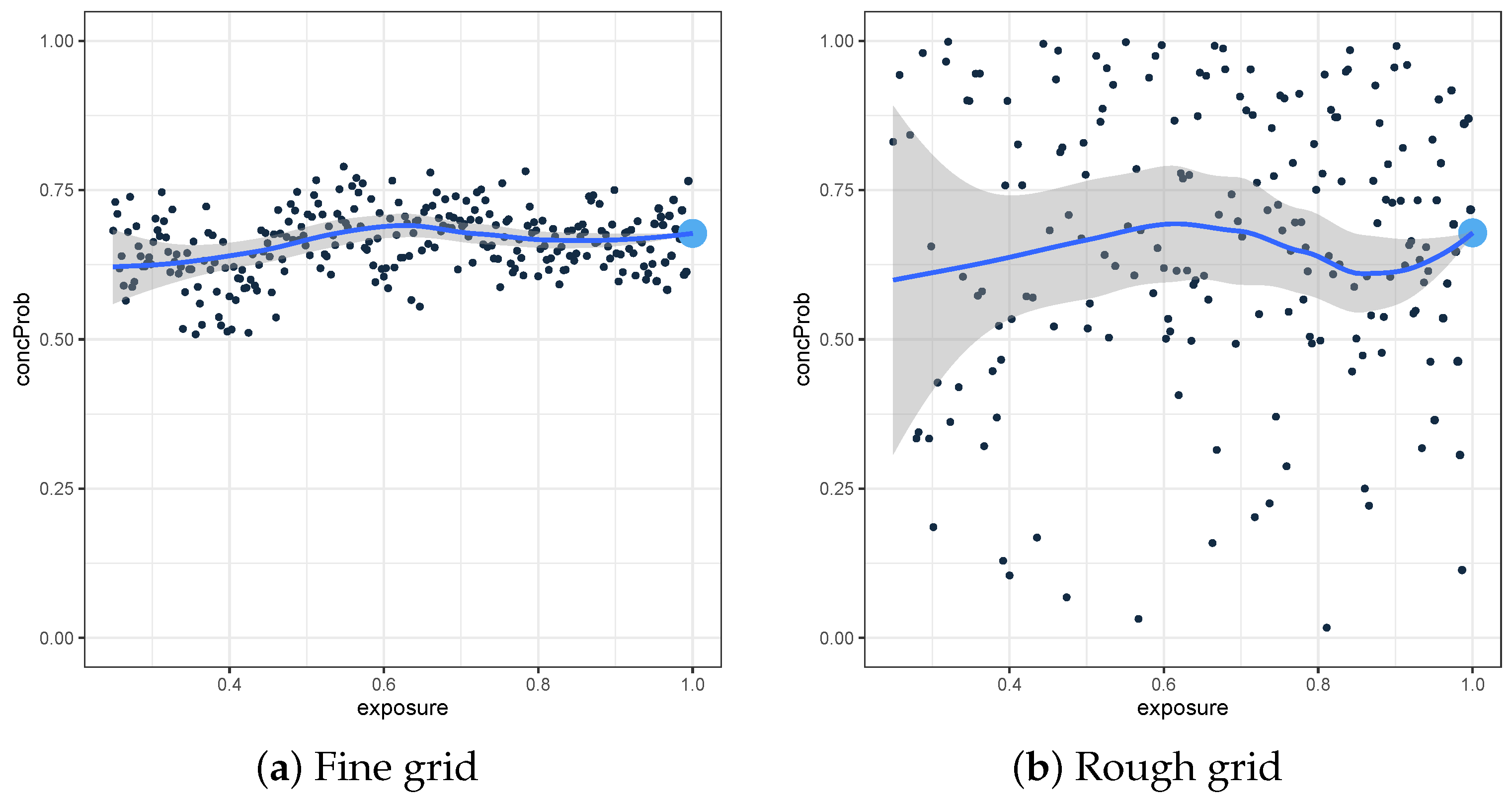
However, the plots are hard to interpret, since there are large differences depending on which group is iterated. Especially in Figure 2, we see that for example C ( 0.08 , 0.05 ) is much larger when iterating over the O -group (fine grid), than when iterating over the 1 -group (rough grid). For the fine grid version, we use the elements of the O -group with exposure equal to 0.08, together with the elements of the 1 -group with an exposure between 0.08 and 0.13. This subset leads to a high value for C ( 0.08 , 0.05 ) , meaning that the selected elements of the 1 -group have in general a higher prediction than the ones of the O -group. However, for the rough grid version, we use the elements of the O -group with an exposure between 0.08 and 0.13, together with the elements of the 1 -group with an exposure equal to 0.08. This is yet another subset, and this time we often see higher predictions for the elements in the O -group, leading to a small value for C ( 0.08 , 0.05 ) . Considering different subgroups, leads to a difficult interpretation of these plots. However, it is important to know that both versions of this local plot lead to the same global concordance probability, based on equality (7).
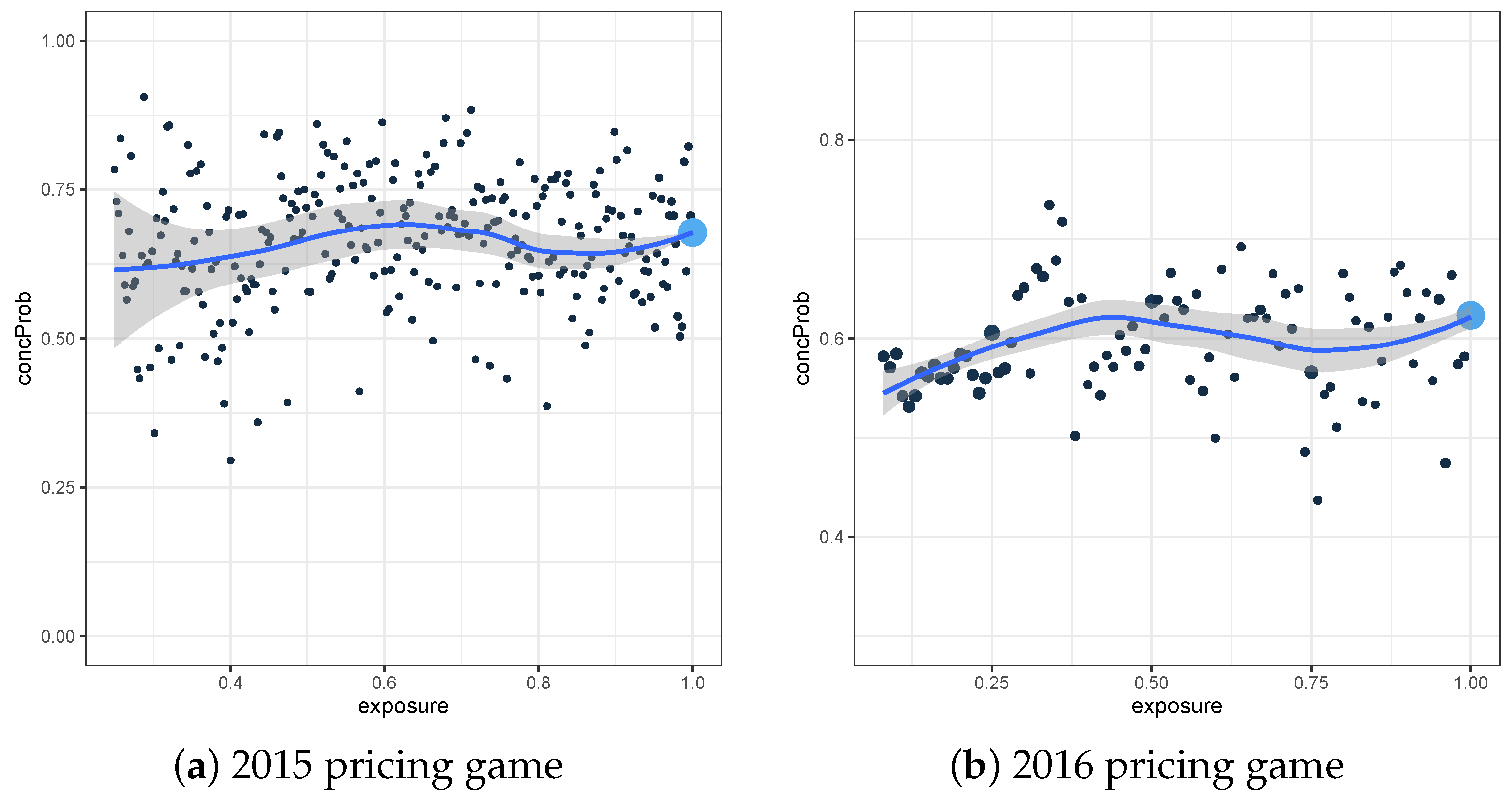
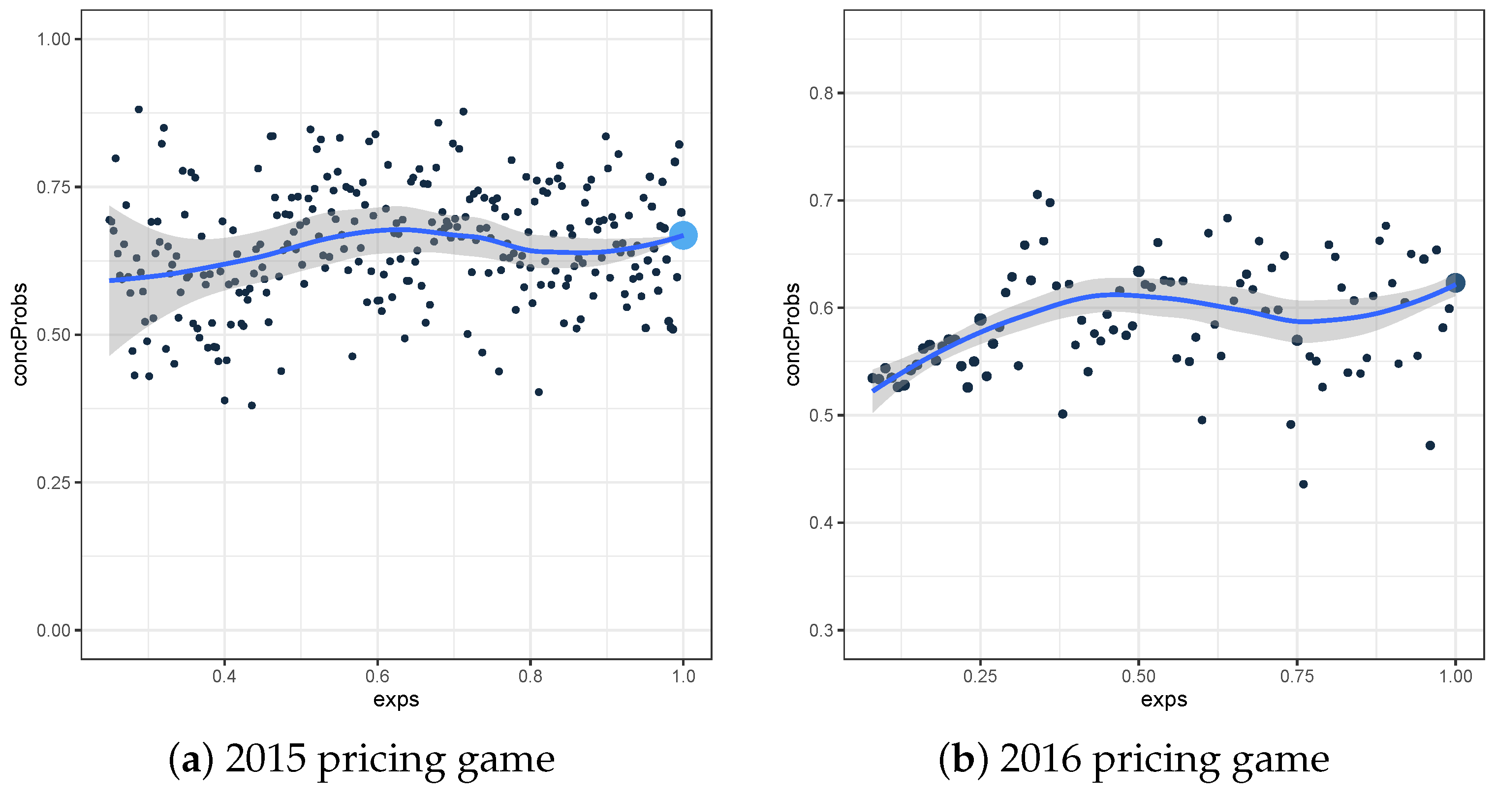
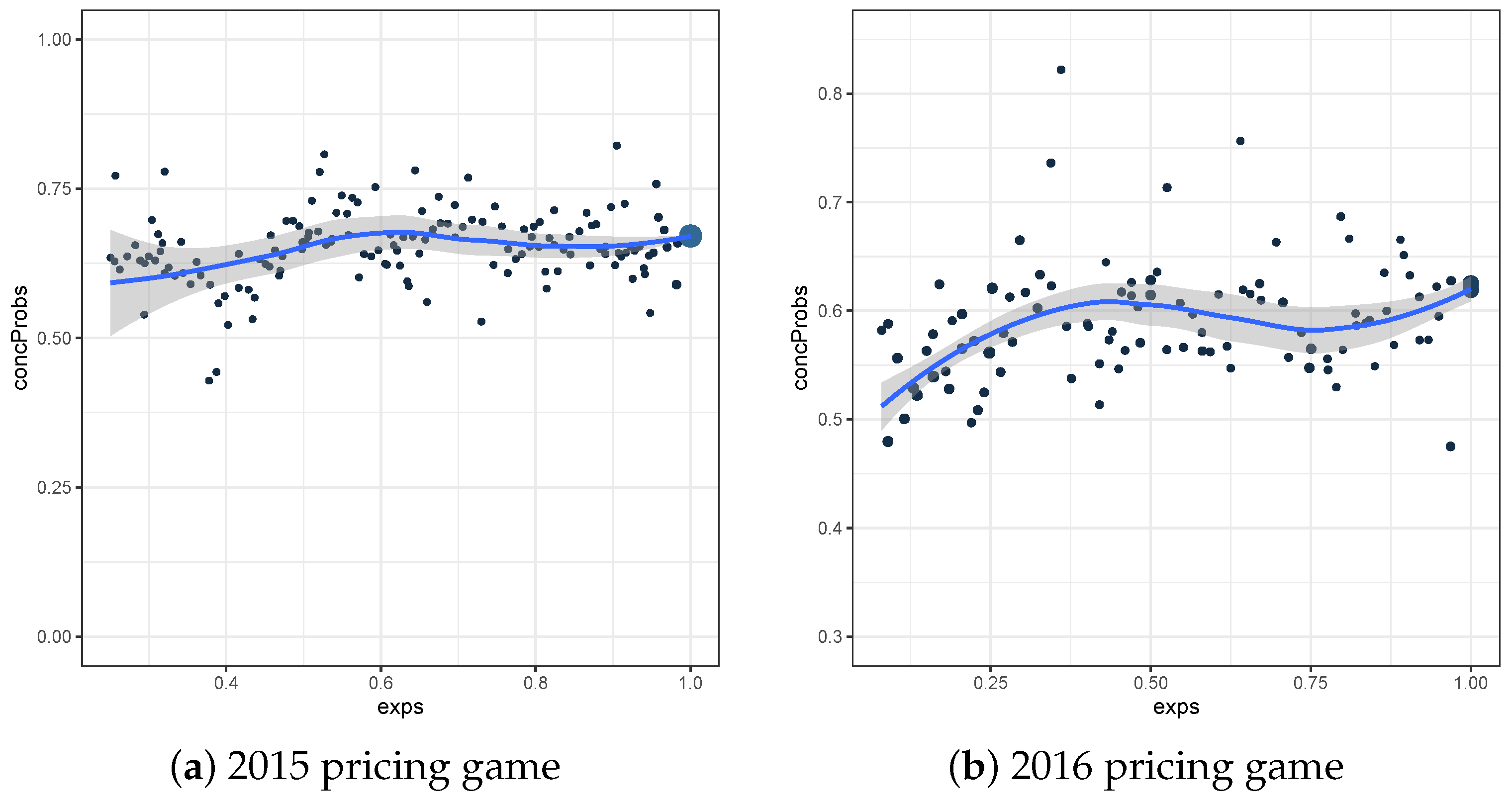
A solution to the lack of interpretability of both local plots (fine and rough grid), is to consider a weighted mean of them, with the weights based on the number of comparable pairs. This weighted-mean-plot is constructed for both datasets and can be seen in Figure 3. For the interpretability, it is important to see that the weighted-mean-plot is equivalent with applying the following two steps:
  • For every observation i, construct C ( λ i , γ ) , with λ i the exposure of the considered element.
  • For every considered exposure λ i , determine the weighted mean of C ( λ i , γ ) , where the weights are based on the total number of comparable pairs.
From Figure 3b, we see that the basic Poisson model for the frequency model based on the dataset of the 2016 pricing game results in small concordance probabilities when considering observations with an exposure around 0.25 or 0.75. Hence, near these exposure values, the model has a hard time distinguishing the two considered groups.

3.2. Severity Models

The general definition (2) of the concordance probability will in this section be modified to a concordance probability that can be used for severity models. Since it might be of little practical importance to distinguish claims from one another that only slightly differ in claim cost, the basic definition can be extended to a version introduced by Van Oirbeek et al. (2021):
C ( ν ) = P π S ( X i ) > π S ( X j ) | Y i S Y j S ν ,
where ν 0 . Furthermore, π S ( · ) refers to the predicted claim size of the severity model and Y S to the observed claim size. In other words, the claims that are to be considered are those of which the claim size has a difference of at least a value ν . Hereby, pairs of claims that makes more sense from a business point of view are selected. Also, a ( ν , C ( ν ) ) plot can be constructed where different values for the threshold ν are chosen, as to investigate the influence of ν on (8). Interestingly, C ( 0 ) corresponds to a global version of the concordance probability (as expressed by definition (2)), while any value of ν > 0 results in a more local version of the concordance probability.
Focusing on the datasets introduced in Section 2, we determine the value of ν such that x% of the pairwise absolute differences of the observed values is smaller than ν , with x { 0 , 20 , 40 } . Note that ν equal to zero is not a popular choice in business, since they are not interested in comparing claims that are nearly identical. The size of the considered test sets still allow to consider all possible pairs between the observations in order to determine the absolute differences between observations belonging to the same pair. However, this is no longer the case for the bootstrapped versions, since this would result in 499,999,500,000 pairs and corresponding differences. Since the observations are all sampled from the original test sets, we know that the number of unique values is much lower than 1,000,000. Hence, we can use the technique discussed in Van Oirbeek et al. (2021), resulting in a fast calculation of the values of ν represented in Table 1. As can be seen, the difference between the values for ν determined on the original test set or on the bootstrapped dataset is very small. Therefore, we will from here on only focus on the bootstrapped versions of the test sets.

4. Time-Efficient Computation

For a sample of size n, the general concordance probability is typically estimated as:
C ^ = n c n t = π ^ c π ^ c + π ^ d = i = 1 n 1 j = i + 1 n I π ^ ( x i ) > π ^ ( x j ) , y i > y j i = 1 n 1 j = i + 1 n I π ^ ( x i ) π ^ ( x j ) , y i > y j ,
corresponding to the ratio of the number of concordant pairs n c over the total number of comparable pairs n t . The value π ^ c ( π ^ d ) refers to the estimated probability that a comparable pair is concordant (discordant) respectively and I ( · ) to the indicator function. Note that the extra condition π ^ ( x i ) π ^ ( x j ) is added to the denominator to ensure that no ties in the predictions are taken into account (Yan and Greene 2008).
Since this estimation method is not possible for large datasets, Van Oirbeek et al. (2021) introduced several algorithms to approximate the concordance probability in an accurate and time-efficient way. We also refer to that article for detailed information and an extensive simulation study. However, new algorithms need to be developed for the frequency setting to approximate the concordance probability dealing with the exposure, and this will be the subject of Section 4.1. For the completeness, we apply the original algorithms of Van Oirbeek et al. (2021) on the severity models in Section 4.2.
In this section, the approximations will be applied to the concordance probability for the models discussed in Section 2.2. More specifically, we will use the bootstrap version such that we have 1,000,000 pairs of observations and predictions to consider.

4.1. Frequency

The goal of this section is to approximate the concordance probability C 0 , 1 + ( 0.05 ) , as defined in (5), in a fast and accurate way. This will be done for the frequency models of Section 2.2, using the 1,000,000 bootstrapped pairs of observations and predictions. Note that the same reasoning can be used for the other concordance probabilities defined in (5).
Before we can determine the bias of the concordance probability estimates, we need to know its exact value. This can be determined by first splitting the considered dataset in the O -group and the 1 -group, as defined in Section 3.1. For the rough grid approach, we iterate over the elements of the 1 -group. In each iteration, we count the number of predictions in the O -group that are smaller than the prediction of the considered element of the 1 -group. Summing up all these counts, divided by the number of considered pairs, results in the exact concordance probability. Contrarily, we iterate over the elements of the O -group for the fine grid approach. In each iteration, we count the number of predictions in the 1 -group that are larger than the prediction of the considered element of the 1 -group. Summing up all these counts, divided by the number of considered pairs, results in the exact concordance probability.
In Table 2, one can see the timings that were necessary to calculate the exact value of C 0 , 1 + ( 0.05 ) , which is 0.6670 (0.5905) for the bootstrap version of the 2015 (2016) pricing game test set. The same was done for C 0 , 1 + ( 0.10 ) , and hence, we can compare both to see the effect of the parameter γ on the run times. We cannot precisely draw a conclusion on the effect of γ on the exact value of the concordance probability, since the exact value of C 0 , 1 + ( 0.10 ) equals 0.6658 (0.5925) for the bootstrap version of the 2015 (2016) pricing game test set. However, for the run times we see clearly larger run times when γ is 0.10. This can be explained by the fact that a larger value for γ implies that we allow more pairs to be compared. Moreover, the run times for the dataset of the 2015 pricing game are clearly larger than the ones for the dataset of 2016. This can be explained by the fact that 73% of the 2015 dataset are observations with an exposure equal to 1. Hence, these observations belong to many comparable pairs. For comparison, only 14% of the observations of the 2016 pricing game dataset have an exposure equal to 1. This is confirmed by Table 3, which shows the number of comparable pairs. From this table, one can also see that the number of comparable pairs for the rough and fine grid approach are equal to each other. This was expected since both approaches result in the exact same global concordance probability. A final note on Table 2 is that it also contains the time to construct the weighted-mean-plot for C 0 , 1 + ( γ ) . Since this plot is constructed as the weighted mean of the fine and the rough grid plot, the time to construct it equals the time to construct both the fine and rough grid plot.

4.1.1. Marginal Approximation

A first approximation for C 0 , 1 + ( 0.05 ) is based on the marginal approximation for discrete variables of Van Oirbeek et al. (2021). More specifically, when we focus f.e. on the fine grid approach, we approximate each local concordance probability C 0 , 1 + ( λ i , 0.05 ) by its marginal approximation, with λ i representing the unique exposures of the O -group. These local approximations are denoted by C ^ M , 0 , 1 + ( λ i , 0.05 ) , such that the first approximation for the global concordance probability C 0 , 1 + ( 0.05 ) is obtained by C ^ M , 0 , 1 + ( 0.05 ) = i w i C ^ M , 0 , 1 + ( λ i , 0.05 ) , with w i representing the same weights as used in (7). A similar reasoning can be used to obtain a marginal approximation for the rough grid approach. Hence, combining both as explained in Section 3.1 results in the weighted-mean-plot approach.
Such a marginal approximation C ^ M , 0 , 1 + ( 0.05 ) takes advantage of the fact that the bivariate distribution of the predictions for considered elements of the O -group and the 1 -group, F π 0 , π 1 ( π O , π 1 ) , is equal to the product of F π O ( π O ) and F π 1 ( π 1 ) . Hence, when a grid with the same q boundary values τ = ( τ 0 , τ 1 , , τ q , τ q + 1 + ) for the marginal distribution of both groups is placed on top of the latter bivariate distribution, the probability that a pair belongs to any of the delineated regions only depends on the marginal distributions F π O ( π O ) and F π 1 ( π 1 ) . Important to note is that Van Oirbeek et al. (2021) took the same q boundary values for each group. These boundary values were a set of evenly spaced quantiles of the empirical distribution of the predictions of both the O -group and the 1 -group jointly. An extension on this idea is that we allow to have different boundary values for each group. Hence, the boundary values of the O -group ( 1 -group) equal the quantiles of the empirical distribution of its predictions. This way of working allows to consider the distribution of each group separately, but the disadvantage is that it will increase the run time. The reason for this increment is that it will be more difficult to determine which region of the grid contains concordant pairs, as can be seen in Figure 4. Therefore, we will compare the original and the extended marginal approximation of the concordance probability C 0 , 1 + ( 0.05 ) for the frequency models of Section 2.2, using the 1,000,000 bootstrapped pairs of observations and predictions.
Table 4 shows the results of the original marginal approximation, hence using the same boundary values for the considered O - and 1 -group when calculating C ^ M , 0 , 1 + ( 0.05 ) . The bias clearly decreases for a higher number of boundary values, but, of course, this coincides with a larger run time. Remarkably, the bias and run time for the marginal approximation of C 0 , 1 + ( 0.05 ) on the bootstrap of the predictions and observations of the 2016 pricing game dataset, are lower than the ones on the 2015 pricing game dataset. A final conclusion on the run times is that, compared to the results in Table 2, the original marginal approximation reduces the run time with at least 50%.
Table 5 shows the results of the extended marginal approximation (weighted-mean-plot approach), hence allowing to have different boundary values for each group. In Appendix C, we see similar results in Table A1 and Table A2 for the fine and rough grid approach respectively. A first conclusion is that when each group has the same number of boundary values, the biases are higher than the ones of the original marginal method. Figure 4 reveals a possible cause, since we clearly see an increase of regions containing incomparable pairs for the extended approach. As a result, the concordance probability is based on fewer comparable pairs, which is confirmed in Table 6. In this situation, we also notice that the run times for the extended marginal approach are comparable with the ones for the original marginal approach, as long as the number of boundary values is smaller than 5000. For a larger number of boundary values, the extended marginal approximation has a higher run time than the original one. In general, we may conclude from Table 5, Table A1 and Table A2 that the bias decreases for a higher number of boundaries, which coincides with a higher run time.
Finally, we also construct an approximation of the weighted-mean-plot for C 0 , 1 + ( λ , 0.05 ) based on the original and extended marginal approximation, respectively shown in Figure 5 and Figure 6. These Figures show the result on the dataset of the 2015 and 2016 pricing game, using 50 boundary values for each group. In Appendix C, one can see nearly identical results in Figure A1 and Figure A2 while using the number of boundary values that resulted in the lowest bias (in case of multiple scenarios, the one with the lowest run time). Comparing these plots with the original ones shown in Figure 3, we see that both the original and the extended marginal approximation give a weighted-mean-plot that is almost the same as the exact one. Based on these plots, the bias and the run time, we have a slight preference for the original marginal approximation where we use the same boundary values for the O -group and the 1 -group.

4.1.2. k-Means Approximation

Another approximation for C 0 , 1 + ( 0.05 ) is based on the k-means approximation for discrete variables of Van Oirbeek et al. (2021). More specifically, when we focus for example on the fine grid version, we approximate each local concordance probability C 0 , 1 + ( λ i , 0.05 ) by its k-means approximation, with λ i representing the unique exposures of the O -group. These local approximations are denoted by C ^ p , k M , 0 , 1 + ( λ i , 0.05 ) , such that the first approximation for the global concordance probability C 0 , 1 + ( 0.05 ) is obtained by C ^ p , k M , 0 , 1 + ( 0.05 ) = i w i C ^ k M , 0 , 1 + ( λ i , 0.05 ) , with w i representing the same weights as used in (7). A similar reasoning can be used to obtain a k-means approximation for the rough grid version. Hence, combining both as explained in Section 3.1 results in the weighted-mean-plot approach.
Such a k-means approximation C ^ k M , 0 , 1 + ( 0.05 ) applies within both groups a k-means clustering algorithm on the considered predictions. Once the clustering algorithms are applied, only the cluster centroids are used to determine C ^ k M , 0 , 1 + ( 0.05 ) . Hence, a more precise estimate will be obtained as k increases. Important to note is that Van Oirbeek et al. (2021) took the same number of clusters for each group. An extension on this idea is that we allow to have a different number of clusters for each group. The results of this extended approximation can be found in Table 7 for the weighted-mean-plot approach. In Appendix D, Table A3 and Table A4 show the results for the fine and rough grid approach respectively. A first conclusion regarding the bias is that it is very low for all considered number of clusters, since a maximum bias of 0.14% was observed over all considered scenarios. This is clearly lower than the comparable bias of the original marginal approximation. However, due to the randomness and the very small values, we do not always see a lower bias for a higher number of clusters. The run time, however, clearly increases for a higher number of clusters. Moreover, these run times are much higher than the ones of the original marginal approximation. Sometimes, they are even higher than the run times to exactly calculate the concordance probability. Despite the rather high run times, the weighted-mean-plots are very close to the exact ones as can be seen in Figure 7 and Figure A3, the latter in Appendix D.
A final approximation for C 0 , 1 + ( 0.05 ) is denoted by C ^ e p , k M , 0 , 1 + ( 0.05 ) and is constructed to have an approximation based on the k-means approximation for discrete variables of Van Oirbeek et al. (2021), without having the high run times as for C ^ k M , 0 , 1 + ( 0.05 ) . These high run times were the result of applying two k-means clustering algorithms for each considered exposure λ i . To determine this new approximation C ^ e p , k M , 0 , 1 + ( 0.05 ) , a k-means clustering algorithm is only applied twice within both groups: first on the exposures and afterwards on the predictions. Hence, only four k-means clustering algorithms are applied. Finally, C ^ e p , k M , 0 , 1 + ( 0.05 ) is obtained by applying Equation (7) on the cluster centroids instead of on the exact exposures and predictions. The results of this third approximation can be found in Table 8 for the weighted-mean-plot approach. In Appendix D, Table A5 and Table A6 show the results for the fine and rough grid approach respectively.
A first important remark is that there are only 275 (93) unique exposures in the 2015 (2016) pricing game dataset. Hence, for a larger number of clusters on the exposures, we have no gain in the run time since we are looping again over all unique exposures. Due to the randomness of selecting the clusters, there is not always a lower bias for a larger number of clusters. Nevertheless, the bias for all considered approximations is very low. More specifically, it is slightly higher than the bias of the corresponding C ^ k M , 0 , 1 + ( 0.05 ) approximation, but still smaller than the one of the original marginal approximation. Finally, we do see an increase in the run time for a larger number of clusters. These run times are clearly smaller than the ones of the corresponding C ^ k M , 0 , 1 + ( 0.05 ) approximation, but still larger than the ones of the original marginal approximation. The weighted-mean-plots are shown in Figure 8 and Figure A4, the latter in Appendix D. Most of these approximations are very close to the exact weighted-mean-plot, apart from the one shown in Figure 8a. There we see that the values around an exposure equal to 0.8 are a bit higher estimated than they should be.
Since the bias of the original marginal approximation is already very low, we do not recommend the k-means algorithm resulting in a lower bias but coinciding with a larger run time. Another important reason for this recommendation, is the fact that more boundary values imply a lower bias for the original marginal approximation, which is not the case for the k-means approximation and its clusters.

4.2. Severity

The goal of this section is to approximate the concordance probability (8) in a fast and accurate way for the severity model of Section 2.2, using the 1,000,000 bootstrapped pairs of observations and predictions.
Before we can determine the bias of the concordance probability estimates, we need to know its exact value. This can be determined by looping over all observations and selecting each time the rows with an observation strictly larger than the considered observation added up with ν . In each iteration, we store the number of selected rows in u . Next, v represents the number of predictions in this selection that are larger than the prediction of the considered element. Finally, the exact concordance probability can be obtained by dividing v ¯ by u ¯ . Important note for this way of working is that we cannot take advantage anymore of the small number of unique values in the observations, since their predictions can differ.
For all considered values of ν , the exact concordance probability is calculated and represented in Table 9 together with its run time. As can be seen for larger values of ν , the concordance probability increases, but the run time decreases. The latter can be explained by the fact that a larger value for ν coincides with fewer comparable pairs. A general conclusion is that it takes a tremendous amount of time to precisely calculate the concordance probability, which is why we will try to approximate these values in a faster way.

4.2.1. Marginal Approximation

A first approximation is the marginal approximation, where a grid is placed on the ( Y S , π ( X ) ) space. The q boundary values τ = ( τ 0 , τ 1 , , τ q , τ q + 1 + ) are evenly spaced percentiles from the empirical distribution of the observed values for Y S and the same set of boundary values is used for dimension π ( X ) . As explained by Van Oirbeek et al. (2021), the marginal approximation of the concordance probability (8) can be computed as:
n C ( ν ) i = 1 q + 1 j = 1 q + 1 n C , τ i j ( ν ) = i = 1 q + 1 j = 1 q + 1 I ( i q , j q ) k = i + 2 q + 1 l = j + 1 q + 1 I ( τ i + ν τ k 1 ) n τ i j , τ k l , n D ( ν ) i = 1 q + 1 j = 1 q + 1 n D , τ i j ( ν ) = i = 1 q + 1 j = 1 q + 1 I ( i q , j 2 ) k = i + 1 q + 1 l = 1 j 1 I ( τ i + ν τ k 1 ) n τ i j , τ k l ,
where τ i j corresponds to the rectangle with values Y S [ τ i 1 , τ i [ and values π ( X ) [ τ j 1 , τ j [ . Furthermore, n C , τ i j ( ν ) ( n D , τ i j ( ν ) ) equals the number of concordant (discordant) comparisons for region τ i j , and n τ i j , τ k l is the product of the number of elements in regions τ i j and τ k l .

4.2.2. k-Means Approximation

Another approximation introduced by Van Oirbeek et al. (2021), is the k-means approximation. For this approximation, the dataset is reduced to a smaller set of clusters that are jointly constructed based on their observed outcomes and predictions. As a result, (8) can be approximated as:
π ^ c i = 1 k 1 j = i + 1 k I π ^ i > π ^ j , y S , i y S , j > ν w i w j ,
π ^ d i = 1 k 1 j = i + 1 k I π ^ i < π ^ j , y S , i y S , j > ν w i w j ,
C ^ k - means ( ν ) = π ^ c π ^ c + π ^ d i = 1 k 1 j = i + 1 k I π ^ i > π ^ j , y S , i y S , j > ν w i w j i = 1 k 1 j = i + 1 k I y S , i y S , j > ν w i w j ,
where y S , l and π ^ l are the observed outcome and the prediction of the representation of the l-th cluster respectively; which is the centroid in case of k-means. w l is the weight of the l-th cluster that is determined by the percentage of observations that pertain to the lth cluster.
The results of the aforementioned approximations can be found in Table 10. There is clearly a smaller bias for a larger number of boundary values or clusters. The disadvantage is that this coincides with a larger run time. There is no considerable connection between the bias and the chosen value for ν . Nevertheless, we do see a shorter run time for higher values of ν , which was already noticed during the exact calculations of the concordance probability and can be explained by the smaller number of comparable pairs. For severity models, we prefer the k-means approximation due to a much smaller run time, combined with a very small bias.

5. Conclusions

Various discrepancy measures and extensions thereof have already been presented in the actuarial literature (Denuit et al. 2019). However, the concordance probability is seldom used in actuarial science, although it is very popular in the machine learning and statistical literature. In this article, we extend the concordance probability to the needs of the frequency and severity data in an insurance context. Both are typically used to calculate the technical premium of a non-life insurance product. For the frequency model, we adapt the concordance probability with respect to the exposure and the fact that the number of claims is not a binary variable. For the severity model, we made sure that claims that are nearly identical in claim cost are not taken into account. The concordance probability measures a model’s discriminatory power and expresses its ability to distinguish risks from each other, a property that is particularly important in non-life insurance. Since it is very time consuming to estimate the above measures for the sizes of frequency and severity data that are typically encountered in practice, several approximations based on computationally efficient algorithms are applied. For the frequency models, we prefer the so-called original marginal approximation, since it has the smallest run time. For these frequency models, it is also possible to visualize the introduced concordance probability in function of the exposure in the so-called weighted-mean-plot. For the severity models, we prefer the k-means approximation due to a small run time combined with a very small bias.

Author Contributions

Conceptualization, J.P. and R.V.O.; methodology, all authors; software, J.P. and R.V.O.; validation, all authors; formal analysis, all authors; investigation, J.P. and R.V.O.; writing—original draft preparation, J.P.; writing—review and editing, R.V.O. and T.V.; visualization, J.P.; supervision, T.V.; funding acquisition, T.V. All authors have read and agreed to the published version of the manuscript.

Funding

This work was supported by the Allianz Research Chair Prescriptive business analytics in insurance at KU Leuven and the International Funds KU Leuven under Grant C16/15/068.

Institutional Review Board Statement

Not applicable.

Informed Consent Statement

Not applicable.

Data Availability Statement

Both datasets are publicly available in the R-package CASdatasets.

Conflicts of Interest

The authors declare no conflict of interest.

Appendix A. Description of the Datasets

For the pg15training dataset, we selected and renamed the following variables:
  • CalYear renamed as uwYear: The underwriting year or the year in which the run time of the policy started. Categorical variable with 2 levels (2009, 2010).
  • Gender renamed as gender: The gender of the car driver. Categorical variable with 2 levels (Male, Female).
  • Type renamed as carType: The car type. Categorical variable with 6 levels (A, B, C, D, E, F).
  • Category renamed as carCat: The car category. Categorical variable with 3 levels (Small, Medium, Large).
  • Occupation renamed as job: The occupation of the driver. Categorical variable with 5 levels (Employed, Housewife, Retired, Self-employed and Unemployed).
  • Age renamed as age: The drivers’ age, expressed in years. Categorized variable with 6 levels (1, 2, …, 6).
  • Group1 renamed as group1: The group of the car. Categorical variable with 20 levels (integer value ranging from 1 to 20, with jumps of 1).
  • Bonus renamed as bm: The bonus-malus or French no-claim discount:−30 means a 30 percent bonus while +20 means a 20 percent malus. Categorical variable with 21 levels (integer value ranging from −50 to 150, with jumps of 10).
  • Poldur renamed as nYears: The number of years that the policy already exists at the beginning of the exposure. Categorical variable with 16 levels (integer value ranging from 0 to 15, with jumps of 1).
  • Value renamed as carVal: The car value in euro. Categorized variable with 6 levels (1, 2, …, 6).
  • Adind renamed as cover: A dummy variable indicating the material cover. Categorical variable with 2 levels (0, 1).
  • Density renamed as density: The population density (number of inhabitants per square km) in the city that the driver of the car lives in. Categorized variable with 6 levels (1, 2, …, 6).
  • Exppdays renamed as exposure: Percentage of a full policy year, corresponding to the run time of the respective policy.
  • Numtpbi renamed as claimNumb: The number of third-party bodily injury claims. The policies for which more than two claims were filed during the considered exposure, the value was set to 2. This adaptation is needed for the measures that are presented in Section 3.
  • Indtpbi renamed as claimCharge: The total cost of third-party bodily injury claims, in euro.
The variables age, carVal and density were originally continuous variables that are transformed to categorical variables as explained by Van Oirbeek et al. (2021).
For the pg16trainpol dataset, we selected and renamed the following variables:
  • Year renamed as covYear: The covering year. Categorical variable with 3 levels (2011, 2012 and 2013).
  • VehiclPower renamed as vehPower: The vehicle power. Categorical variable with 11 levels (P1, P2, …, P11).
  • Deduc renamed as deduc: The deductible category. Categorical variable with 6 levels (0 euro, 1–200 euro, 201–300 euro, 301–400 euro, 401–600 euro, >600 euro).
  • BusinessType renamed as businessType: The business type. Categorical variable with 8 levels (B1, B2, …, B8).
  • ChannelDist renamed as channelDist: The distribution channel. Categorical variable with 3 levels (D1, D2, D3).
  • ClaimNb renamed as claimNumb: The claim number. The policies for which more than two claims were filed during the considered exposure, the value was set to 2. This adaptation is needed for the measures that are presented in Section 3.
  • Exposure renamed as exposure: Percentage of a full policy year, corresponding to the run time of the respective policy.
  • PolicyAgeCateg renamed as age: The category of the policy age. Categorical variable with 6 levels (0–1 year, 1–2 years, 2–3 years, 3–4 years, 4–5 years, >5 years).
  • PolicyCateg renamed as polCat: The category of the policy. Categorical variable with 4 levels (C2, C3, C4, C5).
  • CompanyCreation renamed as compCrea: A dummy indicating if the company has been created.
  • FleetMgt renamed as fleet: The fleet management category. Categorical variable with 2 levels (N, P).
  • FleetSizeCateg renamed as fleetSize: The fleet size category. Categorical variable with 2 levels (S1, S2).
  • Area renamed as area: The geographical area. Categorical variable with 6 levels (A1, A2, …, A6).
  • PayFreq renamed as payFreq: The payment frequency. Categorical variable with 3 levels (quarter, semester, year).
For the pg16trainclaim dataset, we selected and renamed the following variables:
  • DirectComp renamed as matDam: As claims correspond only to material damage, the French claim convention (IDA) was applied. So the insurer may directly refund the insured (matDam=TRUE) even if the insurer will sue the third-party insurer to recover the indemnity afterwards.
  • ClaimCharge renamed as claimCharge: The claim charge.

Appendix B. The Gamma Distribution

The gamma distribution is together with the log-normal distribution and the inverse Gaussian distribution one of the most well-known severity distributions (Denuit et al. 2007). Define Y i j S as the cost of the j t h claim reported by client i, such that Y i S = j Y i j S is its total claim cost. Let all Y i j S be independent random variables following a gamma distribution Gam ( μ i , κ ) with the following density:
f Y i j S ( y i j S ; μ i , κ ) = 1 Γ ( κ ) κ y i j S μ i κ exp κ y i j S μ i 1 y i j S ,
with μ i being the conditional expected cost E[ Y i j S | X i ] and κ is defined such that Var[ Y i j S | X i ] = μ i / κ . Since the corresponding moment generating function is defined by M Y i j S ( t ) = 1 t μ i j κ κ , it follows directly that the average claim cost of client i follows a gamma distribution with mean μ i and variance 1 n i κ μ i 2 , with n i the total number of claims of client i. This corresponds to a gamma distribution with parameters μ i and κ , and weights n i .

Appendix C. Extended and Original Marginal Approximation

Table A1. Bias and run time (s), the latter between brackets, for the extended marginal approximation of C 0 , 1 + ( 0.05 ) on the 2015 and 2016 pricing game dataset. This is given for the fine grid version and for several different numbers of boundary values for the O - and 1 -group.
(a) 2015 Pricing Game
O -Group 1 -Group
501005001000500010,000
500.0067 (2.47)0.0045 (2.39)0.0037 (2.90)0.0036 (3.75)0.0034 (10.55)0.0033 (20.04)
1000.0049 (2.65)0.0033 (2.66)0.0020 (3.28)0.0019 (4.14)0.0017 (12.09)0.0017 (21.82)
5000.0037 (4.36)0.0020 (4.15)0.0007 (4.56)0.0005 (5.74)0.0004 (17.11)0.0004 (32.09)
10000.0035 (6.24)0.0019 (5.70)0.0005 (7.05)0.0003 (7.91)0.0002 (23.57)0.0002 (42.70)
50000.0033 (26.00)0.0017 (23.61)0.0004 (23.24)0.0002 (25.33)0.0001 (69.28)0.0001 (129.04)
10,0000.0033 (49.43)0.0017 (43.43)0.0004 (44.55)0.0002 (46.43)0.0001 (102.01)0.0000 (216.58)
(b) 2016 Pricing Game
O -Group 1 -Group
501005001000500010,000
500.0035 (1.13)0.0028 (1.20)0.0020 (1.50)0.0019 (1.60)0.0018 (3.66)0.0018 (6.47)
1000.0029 (1.19)0.0019 (1.17)0.0011 (1.33)0.0010 (1.67)0.0009 (3.80)0.0009 (7.02)
5000.0019 (1.61)0.0010 (1.78)0.0004 (1.95)0.0003 (2.21)0.0002 (5.89)0.0002 (10.14)
10000.0018 (2.44)0.0010 (2.20)0.0003 (2.44)0.0002 (3.08)0.0001 (8.06)0.0001 (13.81)
50000.0018 (7.86)0.0009 (7.06)0.0002 (7.97)0.0001 (8.15)0.0000 (21.27)0.0000 (41.11)
10,0000.0018 (15.06)0.0009 (13.83)0.0002 (14.35)0.0001 (14.52)0.0001 (32.09)0.0000 (69.49)
Table A2. Bias and run time (s), the latter between brackets, for the extended marginal approximation of C 0 , 1 + ( 0.05 ) on the 2015 and 2016 pricing game dataset. This is given for the rough grid version and for several different numbers of boundary values for the O - and 1 -group.
(a) 2015 Pricing Game
O -Group 1 -Group
501005001000500010,000
500.0068 (5.62)0.0046 (5.62)0.0038 (6.47)0.0035 (7.50)0.0034 (15.30)0.0033 (27.06)
1000.0047 (5.95)0.0032 (6.21)0.0021 (6.72)0.0018 (7.90)0.0017 (16.28)0.0017 (29.97)
5000.0036 (7.59)0.0021 (7.37)0.0007 (8.40)0.0005 (9.71)0.0004 (22.90)0.0003 (38.17)
10000.0034 (8.92)0.0018 (8.43)0.0005 (9.31)0.0003 (11.61)0.0002 (29.47)0.0002 (46.94)
50000.0033 (22.17)0.0017 (19.92)0.0004 (20.60)0.0002 (22.67)0.0001 (70.84)0.0000 (126.75)
10,0000.0033 (38.00)0.0017 (34.24)0.0003 (35.89)0.0002 (37.14)0.0000 (78.37)0.0000 (226.36)
(b) 2016 Pricing Game
O -Group 1 -Group
501005001000500010,000
500.0028 (3.20)0.0024 (3.12)0.0020 (3.34)0.0019 (3.91)0.0018 (6.95)0.0018 (11.12)
1000.0025 (3.26)0.0016 (3.47)0.0011 (3.43)0.0010 (3.83)0.0009 (7.09)0.0009 (11.59)
5000.0019 (3.95)0.0011 (3.90)0.0004 (4.40)0.0003 (5.08)0.0002 (9.25)0.0002 (15.86)
10000.0018 (4.76)0.0010 (4.79)0.0003 (5.05)0.0002 (5.95)0.0001 (11.99)0.0001 (19.85)
50000.0018 (10.48)0.0009 (9.93)0.0002 (10.34)0.0001 (10.65)0.0000 (27.11)0.0000 (50.09)
10,0000.0018 (17.40)0.0009 (15.68)0.0002 (16.31)0.0001 (17.21)0.0001 (36.67)0.0000 (83.13)
Figure A1. Weighted-mean-plot for C ^ M , 0 , 1 + ( λ , 0.05 ) based on the dataset of the 2015 and 2016 pricing game. It is obtained by the original marginal approximation, using the number of boundary values that resulted in the lowest bias.
Risks 09 00178 g0a1
Figure A2. Weighted-mean-plot for C ^ M , 0 , 1 + ( λ , 0.05 ) based on the dataset of the 2015 and 2016 pricing game. It is obtained by the extended marginal approximation, using the number of boundary values that resulted in the lowest bias.
Risks 09 00178 g0a2

Appendix D. k-Means Approximation

Table A3. Bias and run time (s), the latter between brackets, for the approximation C ^ k M , 0 , 1 + ( 0.05 ) on the 2015 and 2016 pricing game dataset. This is given for the fine grid approach and for several different numbers of clusters for the O - and 1 -group.
(a) 2015 Pricing Game
O -Group 1 -Group
50100500
50−0.0024 (11.20)0.0003 (20.28)−0.0002 (88.08)
100−0.0002 (20.37)−0.0001 (37.68)0.0001 (169.08)
5000.0003 (89.36)0.0001 (174.90)0.0000 (810.69)
(b) 2016 Pricing Game
O -Group 1 -Group
50100500
500.0000 (5.17)−0.0001 (7.35)−0.0001 (28.30)
1000.0000 (7.98)−0.0001 (13.14)0.0000 (55.22)
5000.0000 (31.69)0.0000 (56.58)0.0000 (261.58)
Table A4. Bias and run time (s), the latter between brackets, for the approximation C ^ k M , 0 , 1 + ( 0.05 ) on the 2015 and 2016 pricing game dataset. This is given for the rough grid approach and for several different numbers of clusters for the O - and 1 -group.
(a) 2015 Pricing Game
O -Group 1 -Group
50100500
50−0.0004 (25.62)0.0000 (27.02)−0.0002 (28.78)
1000.0000 (35.09)0.0001 (39.66)−0.0001 (38.08)
5000.0000 (107.41)−0.0001 (118.08)0.0000 (121.53)
(b) 2016 Pricing Game
O -Group 1 -Group
50100500
500.0002 (13.19)0.0000 (14.89)−0.0001 (26.54)
100−0.0004 (18.17)0.0001 (23.12)0.0000 (45.57)
5000.0000 (68.81)0.0000 (95.58)0.0000 (206.14)
Table A5. Bias and run time (s), the latter between brackets, for the approximation C ^ e p , k M , 0 , 1 + ( 0.05 ) on the 2015 and 2016 pricing game dataset. This is given for the fine grid approach and for several different numbers of clusters for the O - and 1 -group.
(a) 2015 Pricing Game
O -Group 1 -Group
50100500
50−0.0009 (3.10)−0.0002 (5.63)−0.0001 (9.37)
1000.0011 (6.71)−0.0005 (11.60)−0.0002 (13.84)
500−0.0001 (53.88)0.0003 (104.72)0.0000 (446.11)
(b) 2016 Pricing Game
O -Group 1 -Group
50100500
50−0.0026 (2.19)0.0001 (5.35)−0.0018 (10.68)
1000.0001 (4.46)−0.0003 (7.47)−0.0007 (29.90)
5000.0005 (17.66)−0.0008 (32.20)−0.0007 (143.61)
Table A6. Bias and run time (s), the latter between brackets, for the approximation C ^ e p , k M , 0 , 1 + ( 0.05 ) on the 2015 and 2016 pricing game dataset. This is given for the rough grid approach and for several different numbers of clusters for the O - and 1 -group.
(a) 2015 Pricing Game
O -Group 1 -Group
50100500
50−0.0009 (3.33)−0.0002 (4.30)−0.0001 (12.27)
1000.0011 (4.22)−0.0005 (7.74)−0.0002 (42.37)
500−0.0001 (13.38)0.0003 (27.05)0.0000 (54.50)
(b) 2016 Pricing Game
O -Group 1 -Group
50100500
50−0.0026 (2.97)0.0001 (3.11)−0.0012 (9.97)
1000.0004 (3.70)0.0001 (7.74)−0.0002 (18.08)
5000.0000 (11.11)−0.0003 (30.22)−0.0002 (82.44)
Figure A3. Weighted-mean-plot for C ^ k M , 0 , 1 + ( λ , 0.05 ) based on the dataset of the 2015 and 2016 pricing game. It is obtained by using 100 clusters for each group.
Risks 09 00178 g0a3
Figure A4. Weighted-mean-plot for C ^ e p , k M , 0 , 1 + ( λ , 0.05 ) based on the dataset of the 2015 and 2016 pricing game. It is obtained by using the number of clusters that resulted in the lowest bias.
Risks 09 00178 g0a4

Note

1
http://cas.uqam.ca, accessed on 24 September 2021.

References

  1. Bamber, Donald. 1975. The area above the ordinal dominance graph and the area below the receiver operating characteristic graph. Journal of Mathematical Psychology 12: 387–415. [Google Scholar] [CrossRef]
  2. Denuit, Michel, Xavier Maréchal, Sandra Pitrebois, and Jean-François Walhin. 2007. Actuarial Modelling of Claim Counts: Risk Classification, Credibility and Bonus-Malus Systems. England: John Wiley & Sons. [Google Scholar]
  3. Denuit, Michel, Dominik Sznajder, and Julien Trufin. 2019. Model selection based on lorenz and concentration curves, gini indices and convex order. Insurance: Mathematics and Economics 89: 128–39. [Google Scholar] [CrossRef] [Green Version]
  4. Frees, Edward W. 2009. Regression Modeling with Actuarial and Financial Applications. Cambridge: Cambridge University Press. [Google Scholar]
  5. Frees, Edward W., Richard A. Derrig, and Glenn Meyers. 2014. Predictive Modeling Applications in Actuarial Science. Cambridge: Cambridge University Press, vol. 1. [Google Scholar]
  6. Frees, Edward W., Glenn Meyers, and Richard A. Derrig. 2016. Predictive Modeling Applications in Actuarial Science: Volume 2, Case Studies in Insurance. Cambridge: Cambridge University Press. [Google Scholar]
  7. Legrand, Catherine. 2021. Advanced Survival Models. Boca Raton: CRC Press. [Google Scholar]
  8. Liu, Xu-Ying, Jianxin Wu, and Zhi-Hua Zhou. 2008. Exploratory undersampling for class-imbalance learning. IEEE Transactions on Systems, Man, and Cybernetics, Part B (Cybernetics) 39: 539–50. [Google Scholar]
  9. Ohlsson, Esbjörn, and Björn Johansson. 2010. Non-Life Insurance Pricing with Generalized Linear Models. Berlin and Heidelberg: Springer, vols. 74. [Google Scholar]
  10. Pencina, Michael J., and Ralph B. D’Agostino. 2004. Overall c as a measure of discrimination in survival analysis: Model specific population value and confidence interval estimation. Statistics in Medicine 23: 2109–23. [Google Scholar] [CrossRef] [PubMed]
  11. Reddy, Chandan K., and Charu C. Aggarwal. 2015. Healthcare Data Analytics. Boca Raton: CRC Press, vols. 36. [Google Scholar]
  12. Shi, Peng, Xiaoping Feng, and Anastasia Ivantsova. 2015. Dependent frequency—Severity modeling of insurance claims. Insurance: Mathematics and Economics 64: 417–28. [Google Scholar] [CrossRef]
  13. Steyerberg, Ewout W., Andrew J. Vickers, Nancy R. Cook, Thomas Gerds, Mithat Gonen, Nancy Obuchowski, Michael J. Pencina, and Michael W. Kattan. 2010. Assessing the performance of prediction models: A framework for some traditional and novel measures. Epidemiology 21: 128. [Google Scholar] [CrossRef] [PubMed] [Green Version]
  14. Van Oirbeek, Robin, Emmanuel Jordy Menvouta, Jolien Ponnet, and Tim Verdonck. 2021. Mcube: Multinomial multi-state micro-level reserving model. Submitted. [Google Scholar]
  15. Van Oirbeek, Robin, Jolien Ponnet, and Tim Verdonck. 2021. Computational efficient approximations of the concordance probability in a big data setting. Under Review. [Google Scholar]
  16. Wuthrich, Mario V., and Christoph Buser. 2020. Data analytics for non-life insurance pricing. In Swiss Finance Institute Research Paper. Zurich: Swiss Finance Institute, pp. 16–68. [Google Scholar]
  17. Yan, Guofen, and Tom Greene. 2008. Investigating the effects of ties on measures of concordance. Statistics in Medicine 27: 4190–206. [Google Scholar] [CrossRef] [PubMed]
Figure 1. Plot of the concordance probability C 0 , 1 + ( λ , 0.05 ) in function of the exposure λ , for the frequency model based on the dataset of the 2015 pricing game.
Risks 09 00178 g001
Figure 2. Plot of the concordance probability C 0 , 1 + ( λ , 0.05 ) in function of the exposure λ , for the frequency model based on the dataset of the 2016 pricing game.
Risks 09 00178 g002
Figure 3. Weighted-mean-plot for C 0 , 1 + ( λ , 0.05 ) , constructed as the weighted mean of the fine grid and the rough grid plot.
Risks 09 00178 g003
Figure 4. The different regions of the grid in which the concordant pairs (downward dashed region, in green), the discordant pairs (upward dashed region, in red) and incomparable pairs (upward and downward dashed region, in grey) are highlighted. This is done for the original and the extended marginal approximation.
Risks 09 00178 g004
Figure 5. Weighted-mean-plot for C ^ M , 0 , 1 + ( λ , 0.05 ) based on the dataset of the 2015 and 2016 pricing game. It is obtained by the original marginal approximation, using the same 50 boundary values for the O - and 1 -group.
Risks 09 00178 g005
Figure 6. Weighted-mean-plot for C ^ M , 0 , 1 + ( λ , 0.05 ) based on the dataset of the 2015 and 2016 pricing game. It is obtained by the extended marginal approximation, using 50 boundary values that can differ for the O - and 1 -group.
Risks 09 00178 g006
Figure 7. Weighted-mean-plot for C ^ k M , 0 , 1 + ( λ , 0.05 ) based on the dataset of the 2015 and 2016 pricing game. It is obtained by using the number of clusters that resulted in the highest bias.
Risks 09 00178 g007
Figure 8. Weighted-mean-plot for C ^ e p , k M , 0 , 1 + ( λ , 0.05 ) based on the dataset of the 2015 and 2016 pricing game. It is obtained by using the number of clusters that resulted in the highest bias.
Risks 09 00178 g008
Table 1. The values for ν such that x% of the absolute differences between the observed values is smaller than ν . This is done for the original test set and the bootstrap version, for the datasets of both the 2015 and 2016 pricing game.
(a) 2015 Pricing Game(b) 2016 Pricing Game
x x
0%20%40% 0%20%40%
test0.0000844.112395.93test0.0000377.83825.09
bootstrap0.0000841.442391.00bootstrap0.0000376.63823.88
Table 2. Computing time (s) to calculate the exact concordance probability C 0 , 1 + ( γ ) for the frequency model on the 2015 and 2016 pricing game dataset. This is done for the fine grid, rough grid and weighted-mean-plot approach.
γ Pricing
Game
Fine GridRough GridWeighted-Mean-
Plot
0.052015264.58320.46585.04
201673.4280.12153.54
0.102015286.73331.85618.58
2016115.86132.15248.00
Table 3. The number of comparable pairs that are used to exactly calculate C 0 , 1 + ( γ ) for the frequency model on the 2015 and 2016 pricing game dataset. This is done for the fine grid, rough grid and weighted-mean-plot approach.
γ Pricing
Game
Fine GridRough GridWeighted-Mean-
Plot
0.05201526,539,269,73526,539,269,73553,078,539,470
20165,631,834,0565,631,834,05611,263,668,112
0.10201528,067,838,66028,067,838,66056,135,677,320
20169,023,978,4249,023,978,42418,047,956,848
Table 4. Bias and run time (s), the latter between brackets, for the original marginal approximation of C 0 , 1 + ( 0.05 ) on the 2015 and 2016 pricing game dataset. This is given for the fine grid, rough grid and weighted-mean-plot approach, all for several different numbers of boundary values.
(a) 2015 Pricing Game
Fine GridRough GridWeighted Mean
500.0032 (2.61)0.0033 (5.82)0.0033 (8.43)
1000.0017 (2.83)0.0017 (5.90)0.0017 (8.73)
5000.0003 (6.11)0.0004 (7.42)0.0004 (13.53)
10000.0002 (10.43)0.0002 (9.00)0.0002 (19.43)
50000.0000 (49.08)0.0001 (25.58)0.0001 (74.66)
10,0000.0000 (100.64)0.0001 (47.00)0.0001 (147.64)
(b) 2016 Pricing Game
Fine GridRough GridWeighted Mean
500.0018 (1.38)0.0019 (3.18)0.0018 (4.56)
1000.0009 (1.28)0.0009 (3.17)0.0009 (4.45)
5000.0002 (2.30)0.0002 (4.29)0.0002 (6.59)
10000.0001 (3.89)0.0001 (5.61)0.0001 (9.50)
50000.0001 (18.01)0.0001 (17.27)0.0000 (35.28)
10,0000.0000 (34.46)0.0000 (32.63)0.0000 (67.09)
Table 5. Bias and run time (s), the latter between brackets, for the extended marginal approximation of C 0 , 1 + ( 0.05 ) on the 2015 and 2016 pricing game dataset. This is given for the weighted-mean-plot approach and for several different numbers of boundary values for the O - and 1 -group.
(a) 2015 Pricing Game
O -Group 1 -Group
501005001000500010,000
500.0068 (8.09)0.0045 (8.01)0.0037 (9.37)0.0035 (11.25)0.0034 (25.85)0.0033 (47.10)
1000.0048 (8.60)0.0032 (8.87)0.0020 (10.00)0.0018 (12.04)0.0017 (28.37)0.0017 (51.79)
5000.0036 (11.95)0.0021 (11.52)0.0007 (12.96)0.0005 (15.45)0.0004 (40.01)0.0003 (70.26)
10000.0035 (15.16)0.0019 (14.13)0.0005 (16.36)0.0003 (19.52)0.0002 (53.04)0.0002 (89.64)
50000.0033 (48.17)0.0017 (43.53)0.0004 (43.84)0.0002 (48.00)0.0001 (140.12)0.0000 (255.79)
10,0000.0033 (87.43)0.0017 (77.67)0.0003 (80.44)0.0002 (83.57)0.0001 (180.38)0.0000 (442.94)
(b) 2016 Pricing Game
O -Group 1 -Group
501005001000500010,000
500.0031 (4.33)0.0026 (4.32)0.0020 (4.84)0.0019 (5.51)0.0018 (10.61)0.0018 (17.59)
1000.0027 (4.45)0.0018 (4.64)0.0011 (4.76)0.0010 (5.50)0.0009 (10.89)0.0009 (18.61)
5000.0019 (5.56)0.0011 (5.68)0.0004 (6.35)0.0003 (7.29)0.0002 (15.14)0.0002 (26.00)
10000.0018 (7.20)0.0010 (6.99)0.0003 (7.49)0.0002 (9.03)0.0001 (20.05)0.0001 (33.66)
50000.0018 (18.34)0.0009 (16.99)0.0002 (18.31)0.0001 (18.80)0.0000 (48.38)0.0000 (91.20)
10,0000.0018 (32.46)0.0009 (29.51)0.0002 (30.66)0.0001 (31.73)0.0001 (68.76)0.0000 (152.62)
Table 6. Number of comparable pairs used in the original and extended marginal approximation of C 0 , 1 + ( 0.05 ) on the bootstrap of the predictions and observations of the 2015 and 2016 pricing game dataset. This is done for several different numbers of boundary values.
(a) 2015 Pricing Game(b) 2016 Pricing Game
OriginalExtended
5026,370,518,13325,831,089,271505,282,878,9335,175,036,361
10026,633,484,29426,360,949,9261005,335,780,6755,281,182,645
50026,843,801,54326,788,712,3065005,378,070,4755,366,876,818
100026,870,083,56526,842,431,53710005,383,349,2805,377,637,107
500026,891,057,65126,885,420,71750005,387,563,7525,386,254,164
10,00026,893,659,34726,890,793,88210,0005,388,075,3135,387,331,03
Table 7. Bias and run time (s), the latter between brackets, for the approximation C ^ k M , 0 , 1 + ( 0.05 ) on the 2015 and 2016 pricing game dataset. This is given for the weighted-mean-plot approach and for several different numbers of clusters for the O - and 1 -group.
(a) 2015 Pricing Game
O -Group 1 -Group
50100500
50−0.0014 (36.82)0.0002 (47.30)−0.0002 (116.86)
100−0.0001 (55.46)0.0000 (77.34)0.0000 (207.16)
5000.0001 (196.77)0.0000 (292.98)0.0000 (932.22)
(b) 2016 Pricing Game
O -Group 1 -Group
50100500
500.0001 (18.36)−0.0001 (22.24)−0.0001 (54.84)
100−0.0002 (26.15)0.0000 (36.26)0.0000 (100.79)
5000.0000 (100.5)0.0000 (152.16)0.0000 (467.72)
Table 8. Bias and run time (s), the latter between brackets, for the approximation C ^ e p , k M , 0 , 1 + ( 0.05 ) on the 2015 and 2016 pricing game dataset. This is given for the weighted-mean-plot approach and for several different numbers of clusters for the O - and 1 -group.
(a) 2015 Pricing Game
O -Group 1 -Group
50100500
50−0.0009 (6.43)−0.0002 (9.93)−0.0001 (21.64)
1000.0011 (10.93)−0.0005 (19.34)−0.0002 (56.21)
500−0.0001 (67.26)0.0003 (131.77)0.0000 (500.61)
(b) 2016 pricing game
O -Group 1 -Group
50100500
50−0.0026 (5.16)0.0001 (8.46)−0.0015 (20.65)
1000.0003 (8.16)−0.0001 (15.21)−0.0005 (47.98)
5000.0003 (28.77)−0.0005 (62.42)−0.0004 (226.05)
Table 9. The exact concordance probabilities together with the computing times (s) for different values for ν . The upper (lower) part focuses on the bootstrap version of the test set of the 2015 (2016) pricing game.
(a) 2015 Pricing Game
ν
0841.442391.00
C 0.51750.52020.5242
run time18,420.8616,403.2013,190.45
(b) 2016 Pricing Game
ν
0376.63823.88
C 0.51650.52140.5291
run time17,998.0016,091.0814,088.95
Table 10. The bias and run time (s), the latter between brackets, for the marginal approximation and the k-means approximation of the concordance probability, both for the dataset of the 2015 (a) and 2016 (b) pricing game their severity model.
(a) 2015 Pricing Game
Marginal ν
0.00841.442391.00
500.0014 (18.19)0.0023 (18.48)0.0032 (19.17)
1000.0008 (36.16)0.0012 (37.24)0.0014 (36.88)
5000.0001 (186.86)0.0001 (182.93)0.0001 (183.34)
10000.0001 (367.72)0.0001 (370.40)0.0000 (363.45)
k -means ν
0.00841.442391.00
500.0078 (1.85)0.0045 (1.44)0.0135 (1.41)
1000.0087 (1.59)0.0091 (1.59)0.0150 (1.64)
5000.0008 (4.75)0.0017 (4.52)0.0012 (4.31)
10000.0003 (11.34)0.0005 (10.69)0.0003 (9.64)
(b) 2016 Pricing Game
Marginal ν
0.00376.63823.88
500.0010 (16.91)0.0023 (16.22)0.0024 (16.38)
1000.0010 (32.83)0.0017 (33.01)0.0020 (32.06)
5000.0003 (163.61)0.0005 (154.98)0.0006 (156.66)
10000.0001 (313.95)0.0002 (316.61)0.0003 (329.31)
k -means ν
0.00376.63823.88
500.0140 (1.70)0.0071 (1.04)0.0096 (0.79)
1000.0036 (1.04)0.0029 (1.30)0.0030 (1.14)
500−0.0003 (4.25)0.0009 (4.28)−0.0007 (4.09)
10000.0003 (10.28)−0.0002 (10.00)0.0006 (9.11)
Publisher’s Note: MDPI stays neutral with regard to jurisdictional claims in published maps and institutional affiliations.

