A Genetic Algorithm for Investment–Consumption Optimization with Value-at-Risk Constraint and Information-Processing Cost

Abstract

This paper studies the optimal investment and consumption strategies in a two-asset model. A dynamic Value-at-Risk constraint is imposed to manage the wealth process. By using Value at Risk as the risk measure during the investment horizon, the decision maker can dynamically monitor the exposed risk and quantify the maximum expected loss over a finite horizon period at a given confidence level. In addition, the decision maker has to filter the key economic factors to make decisions. Considering the cost of filtering the factors, the decision maker aims to maximize the utility of consumption in a finite horizon. By using the Kalman filter, a partially observed system is converted to a completely observed one. However, due to the cost of information processing, the decision maker fails to process the information in an arbitrarily rational manner and can only make decisions on the basis of the limited observed signals. A genetic algorithm was developed to find the optimal investment, consumption strategies, and observation strength. Numerical simulation results are provided to illustrate the performance of the algorithm.

1. Introduction

In this paper, we consider an investment–consumption problem. The decision maker manages the investment and consumption with a long-term perspective. General financial information for each investment class is observable. By analyzing the available financial information, the decision maker dynamically allocates the proportion of each investment class to maximize the utilities of consumptions in the long term. The objective under consideration can be traced back to the framework of Merton’s two-asset consumption and investment problem.

Since the financial crisis incurred by the credit risk and the subsequent liquidity risk shocked the banking and insurance system led to a global recession during 2007–2009, regulators and practitioners have paid more attention to risk measurement and management, and numerous techniques have been put forward in the finance and insurance literature. Solvency II, which gradually replaced the Solvency I regime and came into effect on 1 January 2016, is a fundamental review of the capital adequacy regime for the European insurance industry. Value at Risk (VaR) has been widely adopted to quantify and control risk exposure because it is convenient to use. Specifically, it is the maximum expected loss over a finite horizon period at a given confidence level. There are quite a few scholars who have utilized the idea of VaR in the pursuit of deriving optimal risk management strategies (see Yiu 2004; Yiu et al. 2010; Chen et al. 2010; Zhang et al. 2016).

Recent research raises a concern that decision makers generally fail to process all of the information in a rational manner as a result of finite information-processing capability. Under the information-processing constraint, the decision maker can only make decisions through “processed” or “observed” states, which is called “rational inattention”. Sim (2003, 2006) introduced the concept of “rational inattention” and claimed that the process of decision-making is subject to the information-processing constraint. Huang and Liu (2007) investigated the optimal portfolio selection strategies under rational inattention constraints. Maćkowiak and Wiederholt (2015) studied the business cycles within the rational inattention framework and developed a dynamic stochastic general equilibrium model. In addition, it costs to observe the signals and filter the necessary variables. It is natural that the decision maker pays to have a better estimation. Andrei and Hasler (2017) studied the investment and consumption strategies under the rational inattention constraint that an observation cost should be paid to observe key economic factors. See Brennan and Xia (2002), Abel et al. (2013), Steiner et al. (2017), and Kacperczyk et al. (2016) for more work on rational inattention.

Similar to Andrei and Hasler (2017), we also investigate the optimization problem with the information-processing cost. To be specific, in our model, one of the parameters that affect the return of the asset is not observable, thus formulating a partially observable problem. The decision maker can only implement the observable signal to estimate the observable factor. By using the Kalman filter Liptser and Shiryaev (2001), an optimization problem of five state variables and three control variables is formulated. However, our control problem is subject to the Value-at-Risk constraint. The decision maker in our framework controls the consumption, investment, and observation strength to maximize the utilities of consumptions under a given Value-at-Risk requirement.

Our work is also different from Andrei and Hasler (2017) in terms of methodology and research focus. For the research objective, Andrei and Hasler (2017) examined the relationships between attention, risk investment, and related state variables dynamically, whereas our work is dedicated to using an innovative method to achieve the optimal strategies. As for the methodology, Andrei and Hasler (2017) derived the Hamilton–Jacobi–Bellman (HJB) equation for its dynamic system and use the Chebyshev collocation method to approximate the solution of the HJB equation with a sum of certain “basis functions” (in their work, the sum of production of Chebyshev polynomials). Finding the coefficients of Chebyshev polynomials requires solving a system of linear equations. However, the dimension of the derived system of linear equations would increase significantly in our framework with the Value-at-Risk restriction. This limitation motivates us to come up with an alternative method to solve our problem of interest.

Note that the approach applied by Andrei and Hasler (2017) represents one typical way to solve a stochastic control problem, and the method falls into the category of dynamic programming. With dynamic programming, one is able to establish connections between the optimal control problem and a second-order partial differential equation called the HJB equation. If HJB is solvable, then the maximizer or minimizer of the Hamiltonian will be the corresponding optimal feedback control. A more detailed discussion of this field of work can be seen in Yong and Zhou (1999) and references therein. It is very likely that there is no explicit solution to the HJB equation because of the complex nature of a lot of dynamic systems. Thus, the search for effective numerical methods attracts the attention of many scholars accordingly. One common approach follows the track of a numerical method of solving partial differential equations (PDEs; see Andrei and Hasler (2017), for example). Most of the time, it requires good analytical properties such as differentiability and continuity for the dynamic system so that the PDE approach is feasible. The Markov-chain approximation method lies on the other side of the spectrum. It also tackles stochastic control problems but does not require particular analytical properties of the system. This method was proposed by Kushner (see Kushner and Dupuis 2001). The basic idea is to approximate the original control problem with a simpler control process (a Markov chain in a finite state space) and the associated cost function for which the desired computation can be carried out. The state space is a “discretization” of the original state space of the control problem. Under certain conditions, one can prove that the sequence of optimal cost functions for the sequence of approximating chains converges to that for the underlying original process as the approximation parameter goes to zero. A potential problem with the Markov-chain approximation method is that one has to handle the solution of optimization in each iteration step, and this could be time-consuming for high-dimension systems. To deviate from the two popular methods mentioned above, we advocate for the use of Genetic Algorithms to solve stochastic control problems to overcome these issues.

A genetic algorithm (GA) is a metaheuristic inspired by the process of natural selection. Essentially, natural selection acts as a type of optimization process that is based on conceptually simple operations of competition, reproduction, and mutation. Genetic algorithms use these bio-inspired operators (selection, crossover, and mutation) to generate high-quality solutions to optimization problems Mitchell (1996). John Holland introduced genetic algorithms in 1960 on the basis of the concept of Darwin’s theory of evolution; afterward, his student Goldberg extended the GA in 1989 Sadeghi et al. (2014). A fundamental difference between GAs and a lot of traditional optimization algorithms (e.g., gradient descent) is that GAs work with a population of potential solutions of the given problem. The traditional optimization algorithms start with one candidate solution and move it toward the optimum by updating this one estimate. GAs simultaneously consider multiple candidate solutions to the problem of maximizing/minimizing and iterate by moving this population of candidate solutions toward a global optimum. Because of the high dimensionality of parameters and the dynamic constraints in our dynamic system, we developed a Genetic Algorithm to study the optimal strategies.

Note that in recent years, a lot of machine learning methods (both supervised and unsupervised), such as logistic regression, neural networks, support vector machines, k-nearest neighbors, and so on, have been widely used in the field of risk management. These machine learning models are closely related to the problem of optimization since they can be formulated as maximization/minimization of some profit/loss functions. In practical problems, these profit/loss functions tend to be high-dimensional, multi-peak/valley, or may have noise terms, and sometimes they are even discontinuous in some regions. For these situations, a genetic algorithm is a powerful tool for obtaining global optimal solutions. Genetic algorithms have been utilized as optimization methods since the 1980s and 1990s in the field of machine learning (Goldberg and Holland 1988). In many studies, genetic algorithms and machine learning models (such as support vector machines, neural networks) have been used in combination to obtain optimal parameters. On the other hand, machine learning techniques have also been used to improve the performance of genetic and evolutionary algorithms (Zhang et al. 2011).

The contributions of our work are as follows. First, we look at the investment–consumption optimization problem of information cost with the VaR restriction.Second, instead of applying the classical numerical algorithms in which differentiability or continuity assumption is required, we make use of the GA to carry out our analysis. It is very flexible and can handle many types of optimization problems, even if analytical properties such as continuity or differentiability break down. What is more, a lot of numerical algorithms, such as the Markov-chain approximation method, are local optimal algorithms. The GA is a global optimal algorithm instead, and we are thus able to achieve global optimal strategies. Last but not least, the GA is easy to implement and very efficiently handled high-dimensional data.

The rest of the paper is organized as follows. The formulation of the dynamics of wealth inflation, observation processes, and objective functions are presented in Section 2. Numerical examples are provided in Section 3 to illustrate the implementation of the genetic algorithm. Finally, additional remarks are provided in Section 4.

2. Formulation

Let $(\mathsf{\Omega },\mathcal{F},\mathbb{P})$ be a complete probability space, where $\mathcal{F}={\left\{{\mathcal{F}}_t\right\}}_{t\ge 0}$ is a complete and right-continuous filtration generated by a 4-dimensional standard Brownian motion $B_p(t),B_y(t),B_V(t),B_{\beta }(t)$. ${\mathcal{F}}_t$ is the filtration containing the information about the financial market and the investor’s observation at time t, and $\mathbb{P}$ is a probability measure on $\mathsf{\Omega }.$ We consider an asset price process motivated by a fully stochastic volatility model,

$$\frac{dP(t)}{P(t)}=[\overline{\mu }+\beta (t)(y(t)-\overline{y})]dt+\sqrt{V(t)}d{B}_p(t),$$

(1)

where $\overline{\mu }$ is the expected average rate of return. $y(t)$ is an observable state variable that represents useful market information, such as the earnings-to-price ratio or a change in trading volumes to predict the future return rate; $\beta (t)$ is the impact coefficient of the state variable $y(t)$ and is an unobservable factor; $V(t)$ represents the stochastic volatility. Specifically, the observable variable $y(t)$ is assumed to follow a diffusion process

$$:dy(t)={\lambda }_y(\overline{y}-y(t))dt+{\sigma }_y(t)d{B}_y(t).$$

(2)

For the volatility $V(t)$, we adopt the stochastic volatility below:

$$dV(t)={\lambda }_V(\overline{V}-V(t))dt+{\sigma }_V\sqrt{V(t)}d{B}_V(t).$$

(3)

The unobservable factor $\beta (t)$, which can be considered to be certain economic variables that cannot be completely observed, is assumed to follow

$$d\beta (t)={\lambda }_{\beta }(\overline{\beta }-\beta (t))dt+{\sigma }_{\beta }d{B}_{\beta }(t).$$

(4)

Note that for variables $y(t)$, $V(t)$, and $\beta (t)$ above, we use $\overline{y}$, $\overline{V}$, and $\overline{\beta }$ to denote the long-term average of variables and use ${\lambda }_y$, ${\lambda }_V$, and ${\lambda }_{\beta }$ to refer to mean-reversion parameters. These parameters show the rates at which the variables $y(t)$, $V(t)$, and $\beta (t)$ revert to their long-term means in these three mean-reverting processes.

Instead of observing $\beta (t)$ completely, we only have access to the observation of it with noise according to the following dynamics:

$$dO(t)=\beta (t)dt+\frac{1}{\sqrt{\alpha (t)}}d{B}_o(t),$$

(5)

where $B_o(t)$ is a Brownian motion that denotes the observation noises and is independent of $B_p(t),$ $B_y(t),B_V(t),B_{\beta }(t)$. Note that $\alpha (t)$ is a control variable, which determines the precision of our observations and is used to describe the capacity of observing and processing signals. The more frequently we observe the signals, the more precise information we have on the observation. Similarly, a smaller value of $\alpha (t)$ implies less return predictability.

Note that ${\mathcal{F}}_t$ is the information set up to time t and contains the realized return of the asset, innovations of predictive variable, changes in the volatilities of stock return, and observed signals. The estimated predictive coefficient is denoted by $\widehat{\beta }(t)=\mathbb{E}(\beta (t)|{\mathcal{F}}_t)$, and its posterior variance is $\nu (t)=E[{(\beta (t)-\widehat{\beta }(t))}^2|{\mathcal{F}}_t]$. Using the standard filtering results from Liptser and Shiryaev (2001), we are able to get the dynamics of the estimated predictive coefficient $\widehat{\beta }(t)$ (filter) and the posterior variance $\nu (t)$ (uncertainty) as below:

$$d\widehat{\beta }(t)={\lambda }_{\beta }(\overline{\beta }-\widehat{\beta }(t))dt+\frac{\nu (t)(y(t)-\overline{y})}{\sqrt{V(t)}}d{B}_1(t)+\nu (t)\sqrt{\alpha (t)}d{B}_4(t).$$

(6)

$$d\nu (t)/dt=-[\frac{{(y(t)-\overline{y})}^2}{V(t)}+\alpha (t)]{\nu }^2(t)-2{\lambda }_{\beta }\nu (t)+{\sigma }_{\beta }^2.$$

(7)

So far, all state variables have become observable. We thus obtain a new dynamic system with observed variables satisfying the following dynamics:

$$\left\{\begin{array}{c}{\displaystyle \frac{dP(t)}{P(t)}=[\overline{\mu }+\widehat{\beta }(t)(y(t)-\overline{y})]dt+\sqrt{V(t)}d{B}_1(t),}\hfill \\ {\displaystyle dy(t)={\lambda }_y(\overline{y}-y(t))dt+{\sigma }_y(t)d{B}_2(t),}\hfill \\ {\displaystyle dV(t)={\lambda }_V(\overline{V}-V(t))dt+{\sigma }_V\sqrt{V(t)}d{B}_3(t),}\hfill \\ {\displaystyle dO(t)=\widehat{\beta }(t)dt+\frac{1}{\sqrt{\alpha (t)}}d{B}_4(t),}\hfill \end{array}\right.$$

(8)

where $B_1(t),B_2(t),B_3(t)$, and $B_4(t)$ are independent Brownian motions under the investor’s observation filtration.

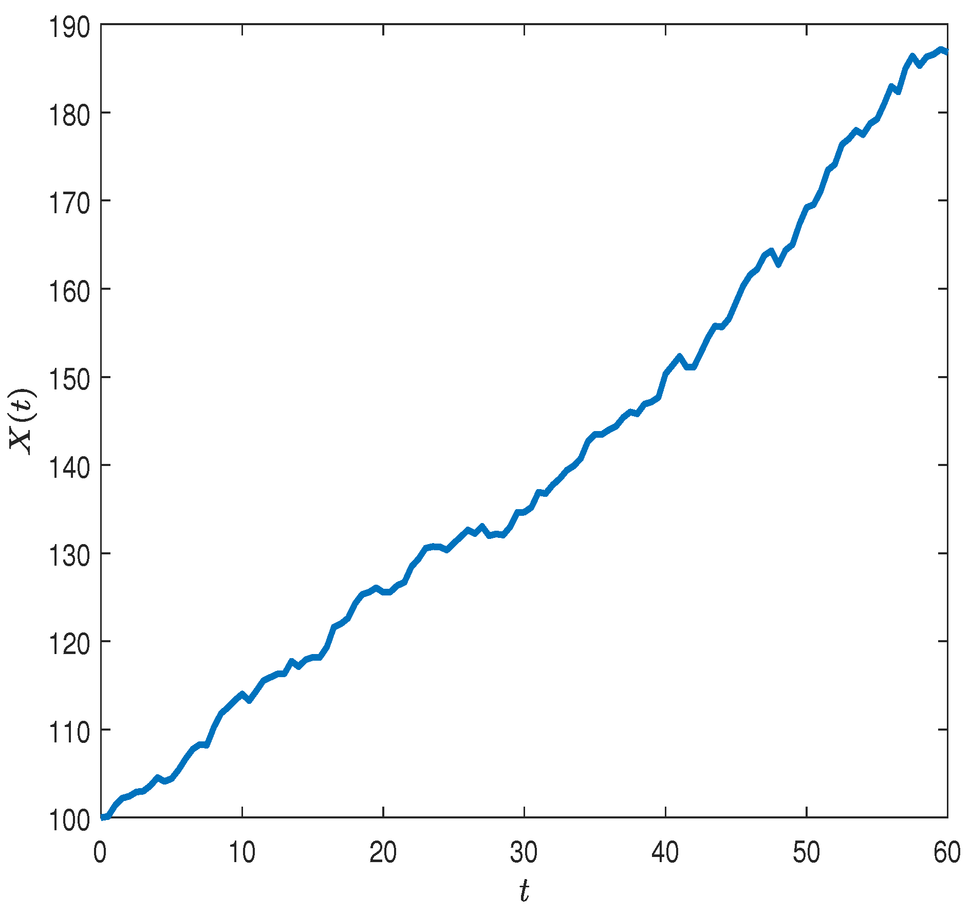
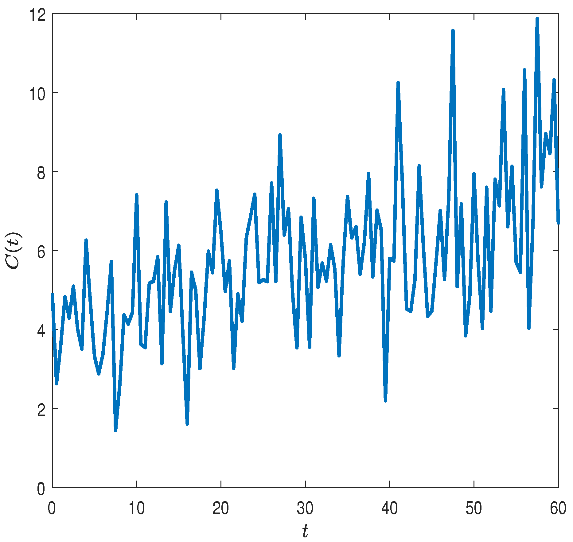
Combining risky assets with a risk-free asset, we can represent the wealth process as:

$$dX(t)=\left[rX(t)+\pi (t)X(t)(\overline{\mu }+\widehat{\beta }(t)(y(t)-\overline{y})-r)-C(t)-\overline{K}(t)\right]dt+\pi (t)X(t)\sqrt{V(t)}d{B}_1(t),$$

(9)

where $C(t)$ is the consumption by a representative investor, consumed at time t; $\pi (t)$ is the risky investment share; r is used to denote the risk-free rate of return; and $\overline{K}(t)$ is the information cost.

Now, we proceed with the introduction of the VaR restriction. Note that with the phenomenal prosperity of financial markets, risk management has recently gained increasing attention from practitioners. Value at Risk has been the standard benchmark for measuring financial risks among banks, insurance companies, and other financial institutions. VaR is regarded as the maximum expected loss over a given time period at a given confidence level and is used to set up capital requirements. VaR constraints have been adopted by many studies on optimization problems to make the model more reasonable. Consistent with Chen et al. (2010), we define the dynamic VaR as follows.

For a small enough $h>0$, the loss percentage in interval $[t,t+h)$ is defined by

$$\Delta X(t):=X(t)e^{rh}-X(t+h).$$

The above definition tells us that relative loss is defined as the difference between the value yielded at time $t+h$ if we deposit the surplus in a bank account at time t and the surplus at time $t+h$ obtained by implementing reinsurance and investment strategies. $e^{rh}$ can be interpreted as the value of time for one unit of currency after time period $h.$

For a given probability level $\varphi \in (0,1)$ and a given time horizon $h>0,$ the VaR at time $t,$ denoted by ${\mathrm{VaR}}_t^{\varphi ,h},$ is defined by

$${\mathrm{VaR}}_t^{\varphi ,h}:=inf\{L\ge 0:\mathbb{P}(\Delta X^{\varphi }(t)\ge L|{\mathcal{F}}_t)<\varphi \}.$$

(10)

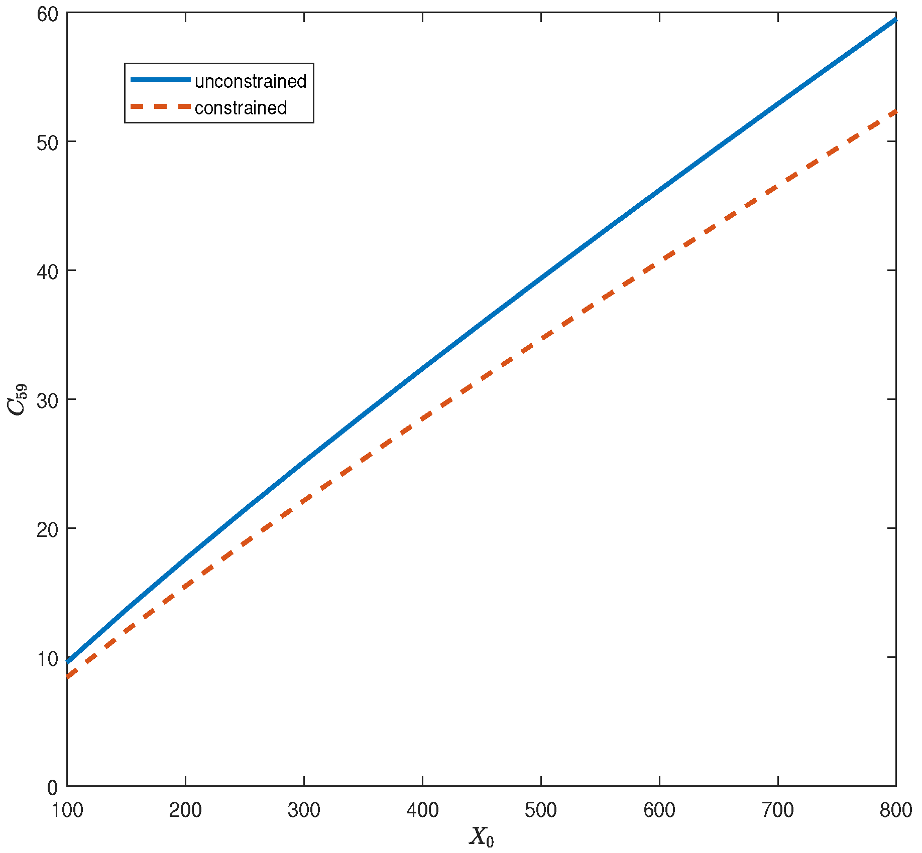
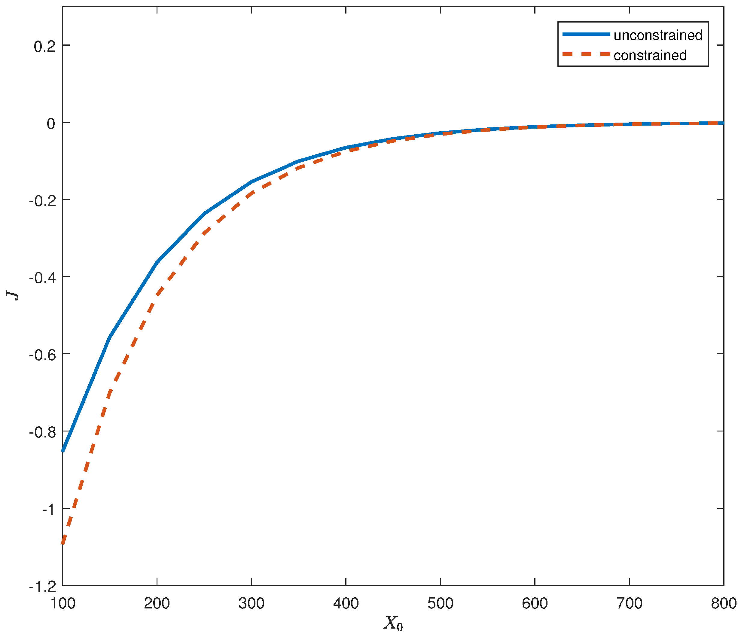
To proceed, let the control variable $u(t)$ be $u(t)=(C(t),\pi (t),\alpha (t))$ as a triplet of control variables. Let $\delta$ be the discount factor. Our objective is to choose consumption $C(t)$, attention to news $\alpha (t)$, and the risky investment share $\pi (t)$ so as to maximize an individual’s expected utility of consumption over a given time horizon from t to T conditional on that individual’s information set at time t:

$$J(t,x,\widehat{\beta },y,V,\nu )=\underset{c,\pi ,\alpha }{max}\mathbb{E}\left[{\int }_t^T{e}^{-\delta (s-t)}U(C_s)ds|{\mathcal{F}}_t\right]$$

(11)

subject to a constant level $R>0$ of an upper boundary of VaR at all times.

$${\mathrm{VaR}}_t^{\varphi ,h}\le R\mathrm{for}\mathrm{a}\mathrm{given}\varphi \mathrm{and}h.$$

(12)

Our interest in this work is the application of a genetic algorithm to solve the optimal investment and consumption strategies in a two-asset model. Compared with some other numerical algorithms, GA is a global optimization method. Moreover, it does not require the differentiability or even continuity of drift and diffusion of the dynamic process. What is more, it is very robust to a change in parameters and easy to implement (Liu and Zhao 1998).

Originating from Darwinian evolution theory, a genetic algorithm can be viewed as an “intelligent” algorithm in which a probabilistic search is applied. In the process of evolution, natural populations evolve according to the principles of natural selection and “survival of the fittest”. Individuals who can more successfully fit in with their surroundings will have better chances to survive and multiply, while those who do not adapt to their environment will be eliminated. This implies that genes from highly fit individuals will spread to an increasing number of individuals in each successive generation. Combinations of good characteristics from highly adapted ancestors may produce even more fit offspring. In this way, species evolve to become progressively better adapted to their environments.

A GA simulates these processes by taking an initial population of individuals and applying genetic operators to each reproduction. In optimization terms, each individual in the population is encoded into a string or chromosome or some float number, which represents a possible solution to a given problem. The fitness of an individual is evaluated with respect to a given objective function. Highly fit individuals or solutions are given opportunities to reproduce by exchanging some of their genetic information with other highly fit individuals by a crossover procedure. This produces new “offspring” solutions (i.e., children), which share some characteristics taken from both parents. Mutation is often applied after crossover by altering some genes or perturbing float numbers. The offspring can either replace the whole population or replace less-fit individuals. This evaluation-selection-reproduction cycle is repeated until a satisfactory solution is found. The basic steps of a simple GA are shown below and in the next section, and we define the detailed steps of the GA after a specific example is introduced.

• Generate an initial population and evaluate the fitness of the individuals in the population;
• Select parents from the population;
• Crossover (mate) parents to produce children and evaluate the fitness of the children;
• Replace some or all of the population by the children until a satisfactory solution is found.

3. Numerical Simulation with Genetic Algorithm

3.1. Numerical Example

Andrei and Hasler (2017) investigated the determinants of optimal attention and risky investment share, and they calibrated the parameter of the model. Another major focus of their work concerns the exploration of the relation between the model-implied and empirically measured attention and risky investment. Our focus in this work is quite different, and we aim to shed light on the application of the GA to a constrained stochastic control problem. In this section, we numerically apply the GA to a specific example in order to provide a visualized understanding of optimal attention behavior, consumption, as well as an investor’s portfolio selection for maximizing its utility function over time. For the sake of convenience, we used the estimated parameters out of Andrei and Hasler (2017) to proceed with our simulations below. To be more specific,

$$r=0.0508,{\lambda }_V=1.9592,X_0=100,\overline{V}=0.0158,$$

$${\sigma }_V=0.176,{\lambda }_y=0.1163,\overline{y}=0.0686,{\sigma }_y(t)={\sigma }_y=0.0136,$$

$$\overline{\mu }=0.0685,{\lambda }_{\beta }=0.2151,\overline{\beta }=0.0021,{\sigma }_{\beta }=0.9531.$$

$$\left\{\begin{array}{c}{\displaystyle \frac{dP(t)}{P(t)}=[0.0685+\widehat{\beta }(t)(y(t)-0.0686)]dt+\sqrt{V(t)}d{B}_1(t),}\hfill \\ {\displaystyle dy(t)=0.1163(0.0686-y(t))dt+0.0136d{B}_2(t)}\hfill \\ {\displaystyle dV(t)=1.9592(0.0158-V(t))dt+0.176\sqrt{V(t)}d{B}_3(t),}\hfill \\ {\displaystyle dO(t)=\widehat{\beta }(t)dt+\frac{1}{\sqrt{\alpha (t)}}d{B}_4(t),}\hfill \\ {\displaystyle d\widehat{\beta }(t)=0.2151(0.0021-\widehat{\beta }(t))dt+\frac{\nu (t)(y(t)-0.0686)}{\sqrt{V(t)}}d{B}_1(t)+\nu (t)\sqrt{\alpha (t)}d{B}_4(t),}\hfill \\ {\displaystyle d\nu (t)/dt=-[\frac{{(y(t)-0.0686)}^2}{V(t)}+\alpha (t)]{\nu }^2(t)-0.4302\nu (t)+{0.9531}^2.}\hfill \end{array}\right.$$

(13)

Thus, our corresponding wealth processes can be represented as below:

$$\begin{array}{cc}dX(t)\hfill & {\displaystyle =[0.0508X(t)+\pi (t)X(t)(0.0685+\widehat{\beta }(t)(y(t)-0.0686)-0.0508)}\hfill \\ \hfill & {\displaystyle -\eta (t)X(t)-0.1{\alpha }^2(t)X(t)]dt+\pi (t)X(t)\sqrt{V(t)}d{B}_1(t),}\hfill \\ X(0)\hfill & {\displaystyle =100.}\hfill \end{array}$$

(14)

Here, we naturally assume that consumption is a proportion of wealth $C(t)=\eta (t)X(t)$ and that the per unit of wealth information cost function is $\overline{K}(t)=k{\alpha }^2(t)$. The information cost parameter k is assumed to be $k=0.1$. Thus, we need to choose the control set $u(t)=(\eta (t),\pi (t),\alpha (t))$ to maximize our utility function. To be specific, we adopted the power utility function $U(C):=\frac{C^{1-\gamma }}{1-\gamma }$ for the simulation, in which we further assume that the value of the aversion parameter is $\gamma =3$. The time window is assumed to be 60 years. Then, we have

$$J(x,\widehat{\beta },y,V,\nu )=max\mathbb{E}\left[{\int }_0^{60}-e^{-0.01t}\frac{C_t^{-2}}{2}dt\right]$$

(15)

subject to

$${\mathrm{VaR}}_t^{\varphi ,h}\le 0.1X(t),$$

(16)

where the discount factor takes the value of $\delta =0.01$ and $\varphi =0.01$. To proceed with our numerical analysis, we used step size $\Delta t=h=1/2$ and simulated the trajectory $10,000$ times. Realizing that relative loss is actually more meaningful since the impact of a $10,000 loss differs between a billionaire and a junior investor. Therefore, in our example, we did not choose a specific upper bound for the VaR. Instead, we restricted the loss portion to be less than 10% of the wealth to proceed with our simulation, and the constant upper bound of the VaR can be regarded as a special case of our example.

3.2. Implementation of GA

Note that there are a lot of variations of genetic algorithms. To solve our problem of interest, we can use the form along the lines of what Liu and Zhao (1998) suggested in their book. Below are the specifics of the basic steps of our GA.

Step 1:

Set parameters $P_c=0.2$ (probability of crossover), $P_m=0.1$ (probability of mutation), $N=30$ (size of population), $b=0.05$ (the parameter used in the evaluation); set iteration $iter:=0$, $best:=0$.

Step 2:

Initialize population $pop(iter)=\{{\theta }_1,\dots ,{\theta }_N\}$, which is a population that contains N solutions. In our context, ${\theta }_i=({\eta }_1,\dots ,{\eta }_{120},{\pi }_1,\dots ,{\pi }_{120},{\alpha }_1,\dots ,{\alpha }_{120})$, ${\eta }_j$, ${\pi }_j$, and ${\alpha }_j$ ($j=1,\dots ,120$) are three random controls following a uniform distribution $U(0,1)$. Note that our time window is 60 years and the step size is 1/2; thus, each control variable can be discretized from $j=1$ up to $j=120$.

Step 3:

Evaluate $pop(iter):\{{\theta }_1,\dots ,{\theta }_N\}$:

3-1:

For each ${\theta }_i$, plug ${\theta }_i$ into the discretized form of Equation (15).

3-2:

Descending sort $\{J({\theta }_1),\dots ,J({\theta }_N)\}$; for the sake of brevity, we assume $J({\theta }_1)\ge J({\theta }_2)\ge \cdots \ge J({\theta }_N)$. If $best<J({\theta }_1)$, then denote the best value as $best=J({\theta }_1)$ and store ${\theta }_1$.

3-3:

If the stop criterion $iter=1000$ is satisfied, output ${\theta }_1$ and the best value $best$ and stop the genetic algorithm. Otherwise, continue the algorithm.

3-4:

Evaluate each ${\theta }_i$ by

$$eval({\theta }_i)=b{(1-b)}^{i-1}.$$

Step 4:

Selection:

   

For$i:=1$toN

4-1:

For each ${\theta }_i$, calculate the cumulative probability $q_i$

$$\left\{\begin{array}{c}{q}_0=0,\hfill \\ q_i={\displaystyle \sum _{j=1}^i}eval({\theta }_j)i=1,2,\dots ,N\hfill \end{array}\right.$$

4-2:

Generate a random number $r\sim U(0,q_N)$;

4-3:

If $q_{i-1}<r\le q_i$, then choose the ith individual ${\theta }_i$, and let ${\theta }_i^{\prime }\leftarrow {\theta }_i$;

   

End For (Here, we can obtain N individuals ${\theta }_1^{\prime },\dots ,{\theta }_N^{\prime }$).

Step 5:

Crossover:

   

For$i:=1$toN

5-1:

Generate a random number $r\sim U(0,1)$;

5-2:

Choose ${\theta }_i^{\prime }$ as a parent if $r<P_c$, and let $V_i\leftarrow {\theta }_i^{\prime }$;

   

End For (Here, we can obtain k ($k\le N$) parents $V_1,\dots ,V_k$).

5-3:

Partition $\{V_1,\dots ,V_k\}$ into $k/2$ pairs randomly $(V_1,V_2),(V_3,V_4),\dots$ (if k is odd, we can discard an arbitrary one).

5-4:

Generate another random number $d\sim U(0,1)$; for each pair $(V_i,V_{i+1})$, we can get two new individuals by

$$\begin{array}{c}X=d{V}_i+(1-d)V_{i+1}\hfill \\ Y=(1-d)V_i+d{V}_{i+1}\hfill \\ V_i\leftarrow X\hfill \\ V_{i+1}\leftarrow Y\hfill \end{array}$$

5-5:

Use $\{V_1,\dots ,V_k\}$ to replace k individuals in $\{{\theta }_1^{\prime },\dots ,{\theta }_N^{\prime }\}$.

Step 6:

Mutation:

   

For$i:=1$toN

6-1:

Generate a random number $r\sim U(0,1)$;

6-2:

If $r<P_m$, generate an individual $V_i^{\prime }=({\eta }_1,\dots ,{\eta }_{120},{\pi }_1,\dots ,{\pi }_{120},{\alpha }_1,\dots ,{\alpha }_{120})$ and let ${\theta }_i^{\prime }\leftarrow V_i^{\prime }$; ${\eta }_j$, ${\pi }_j$, and ${\alpha }_j$ are three random controls following a uniform distribution $U(0,1)$. Then, let ${\theta }_i^{\prime }\leftarrow V_i^{\prime }$;

   

End For

Step 7:

Now, a new population $\{{\theta }_1^{\prime },\dots ,{\theta }_N^{\prime }\}$ is obtained. Let ${\theta }_i\leftarrow {\theta }_i^{\prime }$, $iter\leftarrow iter+1$, and go to Step 3.

Remark 1.

Note that in Steps 2 and 6 above, both ${\theta }_i$ and $V_i^{\prime }$ refer to the ith generic feasible solution from a population of size N for the optimization problem, and they have different appearances in different contexts.

In Figure 1 and Figure 2, we see both consumption and average wealth have a trend of increasing over 60 years. Given that our utility function is in terms of consumption, the investor has the motivation to increase consumption. On the other hand, if the investor consumes too much, his/her wealth tends to go down, and this will result in less wealth to be spent on consumption in the future. Therefore, there exists a trade-off. Overall, an investor’s wealth goes up relatively smoothly over the course of time, but there are ups and downs in terms of the trajectory of consumption. We think this fits the reality since a rational investor tends to spend more sometimes as a result of purchasing some big tangible assets, such as a car or house, or health concerns; at other times, an investor spends less money on living expenses. In Figure 3, we further examine the consumption pattern by studying $\eta (t)$. Recall that $\eta (t)$ is the proportion of wealth that an investor spends on consumption. We find that the optimal proportion of consumption $\eta (t)$ is bounded between $0.0134$ and $0.0704$. The optimal proportion of consumption for a rational investor under the VaR restriction is stable in the long term and would not exceed $8\%$ of the investor’s wealth.

For experts familiar with finance theory, the range of the optimal proportion of consumption might look a bit fishy at first glance since it seems to conflict with the famous frugal 4% consumption rule from the “Trinity study” (Cooley et al. 1998). However, Bengen (1994) showed that the 4% consumption rule is suggested for the first year, and the proportion should be adjusted up or down for inflation every succeeding year. Checking our proposed optimal consumptions, the optimal proportion of consumption takes an average value of 3.775% for the first year. The mean and volatility (standard deviation) of optimal consumption are 4.09% and 1.14%, respectively. Figure 4 shows that 62% of the optimal consumptions fall within [0.0295, 0.0523]. We also notice that 2.48% of the optimal consumptions fall below 0.018, and 3.31% of consumptions are above $0.0637$. Thus, we claim that, overall, our numerical results agree with the conclusion of the “Trinity study” well, and the corresponding relative frequencies of large deviations from the “canonical” results are very small. Considering the existing fluctuations in our optimal consumptions, we guess that inflation, the cost of information processing, and random noise could all be contributing factors. That being said, theories from the field of behavioral finance, such as habit formation proposed by Constantinides (1990) and Abel (1990) and the equity risk puzzle discussed by Mehra (2006), could also be underlying driving forces.

Figure 5 and Figure 6 demonstrate the dynamics of optimal proportion of risky assets and optimal attention cost with respect to time. Checking the graphs, we can see that $\pi (t)\in [0.0130,0.0683]$ and $\alpha (t)\in [0.0078,0.0747]$. Putting the three control variables together, we see that to maximize the utility function, the investor should put most of his/her wealth in risk-free assets and increase consumption over the course of time so that the wealth can accumulate in a steady way; thus, the investor is able to spend more money on consumption. When the utility function is consumption oriented, there is less incentive for the investor to invest more money in risky assets because of the embedded risk. Thus, the optimal proportion of wealth in the risky asset is not very aggressive.

To see the impact of the VaR restriction, we examined the optimal consumption for a case with and without VaR restrictions with respect to initial wealth $X_0$. We locked the time to year 1 and 59, respectively, to make comparisons. Figure 7 and Figure 8 reveal the following observations. First, the consumptions in both graphs increase as the initial wealth goes up. Second, investors consume more when there is no restriction. The constraint of VaR serves as a buffer to stop an investor from spending more money. Last but not least, examining the consumption patterns under VaR, we notice that in the early stage of our time window of interest, the consumption under VaR is convex from below as a function of initial wealth. However, the shape becomes slightly concave from below in the end. A possible explanation is that in the beginning, more wealth implies higher consumption, but there is a diminishing marginal utility here, and the investor is risk seeking. However, toward the end of the time horizon, a rational investor will spend as much as possible, as more wealth implies more consumption, and moreover, marginal consumption goes up and the risk aversion part of investor is dominant.

Figure 9 is along the lines of a comparison between the constrained and unconstrained optimization problem, but the focus is on the relationship between the value function and initial wealth. Our numerical result shows that the investor gets a higher utility function when there is no VaR constraint. It is also very interesting to note that the gap between the utility functions is apparent when the initial wealth is small. However, as the initial wealth increases, the gap between the utility functions becomes narrow. In the beginning, the VaR restriction really acts as a restriction because the initial wealth is assumed to be small. Investors will be very careful about their investment strategies and will thus consume conservatively. As the initial wealth increases, while the utility function for the unconstrained case is still higher, it is close to that of the constrained case. It shows that the VaR restriction does not have a substantial influence for a “rich” investor.

4. Concluding Remarks

In this paper, we present a genetic algorithm to study the optimal consumption and investment strategies for a decision maker whose decision-making is subject to the Value-at-Risk constraint. Because of the partial observability of the return rate of risky assets, the decision maker needs to filter the key economic factors at a cost to maximize the objective function. The observation strength, which requires a trade-off between accuracy and cost, is a control variable to determine. Since solving the high-dimension Hamilton–Jacob–Bellman (HJB) equation analytically is virtually impossible, we developed a genetic algorithm to solve the problem numerically. The numerical simulations yield some interesting observations. In future studies, we can further consider the information-processing capacity constraint of the decision maker. The decision maker has a finite signal-processing capacity to filter the true states with a cost. We can use entropy to quantify the information-processing capacity for decision makers. Luo (2016) analyzed optimal consumption and portfolio strategies with the information-processing capacity constraint. It was shown that the limit imposed by rational inattention has a significant effect on the decision-making process. Together with the Value-at-Risk constraint, the problem becomes more complex and leads to a Hamilton–Jacob–Bellman equation of much higher dimensions. A more advanced algorithm will be studied to tackle the difficulty with high dimensions.

References

1. Abel, Andrew B. 1990. Asset prices under habit formation and catching up with the joneses. The American Economic Review 80: 38–42. [Google Scholar]
2. Abel, Andrew B., Janice C. Eberly, and Stavros Panageas. 2013. Optimal inattention to the stock market with information costs and transactions costs. Econometrica 81: 1455–81. [Google Scholar]
3. Andrei, Daniel, and Michael Hasler. 2017. Dynamic Attention Behavior Under Return Predictability. Working Paper. Available online: http://www-2.rotman.utoronto.ca/facbios/file/AH3_20170429.pdf (accessed on 22 January 2019).
4. Bengen, William P. 1994. Determining withdrawal rates using historical data. Journal of Financial Planning 1: 14–24. [Google Scholar]
5. Brennan, Michael J., and Yihong Xia. 2002. Dynamic asset allocation under inflation. The Journal of Finance 57: 1201–38. [Google Scholar] [CrossRef]
6. Chen, Shumin, Zhongfei Li, and Kemian Li. 2010. Optimal investment-reinsurance policy for an insurance company with VaR constraint. Insurance: Mathematics and Economics 47: 144–53. [Google Scholar] [CrossRef]
7. Constantinides, George M. 1990. Habit formation: A resolution of the equity premium puzzle. Journal of Political Economy 98: 519–43. [Google Scholar] [CrossRef]
8. Cooley, Philip L., Carl M. Hubbard, and Daniel T. Walz. 1998. Retirement savings: Choosing a withdrawal rate that is sustainable. AAII Journal 10: 16–21. [Google Scholar]
9. Goldberg, David E., and John H. Holland. 1988. Genetic algorithms and machine learning. Machine Learning 3: 95–99. [Google Scholar] [CrossRef]
10. Huang, Lixin, and Hong Liu. 2007. Rational inattention and portfolio selection. The Journal of Finance 62: 1999–2040. [Google Scholar] [CrossRef]
11. Kacperczyk, Marcin, Stijn Van Nieuwerburgh, and Laura Veldkamp. 2016. A rational theory of mutual funds’ attention allocation. Econometrica 84: 571–626. [Google Scholar] [CrossRef]
12. Kushner, Harold J., and Paul Dupuis. 2001. Numerical Methods for Stochastic Control Problems in Continuous Time. Berlin: Springer. [Google Scholar]
13. Liptser, Robert S., and Albert N. Shiryaev. 2007. Statistics of Random Processes, II: Applications. Berlin: Springer. [Google Scholar]
14. Liu, Baoding, and Ruiqing Zhao. 1998. Stochastic Programming and Fuzzy Prgramming. Beijing: Tsinghua University Press. [Google Scholar]
15. Luo, Yufei. 2016. Robustly strategic consumption-portfolio rules with informational frictions. Management Science 63: 4158–74. [Google Scholar] [CrossRef]
16. Maćkowiak, Bartosz, and Mirko Wiederholt. 2015. Business cycle dynamics under rational inattention. The Review of Economic Studies 82: 1502–32. [Google Scholar] [CrossRef]
17. Mehra, Rajnish. 2006. The equity premium puzzle: A review. Foundations and Trends in Finance 2: 1–81. [Google Scholar] [CrossRef]
18. Mitchell, Melanie. 1996. An Introduction to Genetic Algorithms. Cambridge: MIT Press. [Google Scholar]
19. Sadeghi, Javad, Saeid Sadeghi, and Seyed Taghi Akhavan Niaki. 2014. Optimizing a hybrid vendor-managed inventory and transportation problem with fuzzy demand: An improved particle swarm optimization algorithm. Information Sciences 272: 126–44. [Google Scholar] [CrossRef]
20. Sims, Christopher A. 2003. Implications of rational inattention. Journal of Monetary Economics 50: 665–90. [Google Scholar] [CrossRef]
21. Sims, Christopher A. 2006. Rational inattention: Beyond the linear-quadratic case. The American Economic Review 96: 158–63. [Google Scholar] [CrossRef]
22. Steiner, Jakub, Colin Stewart, and Filip Matĕjka. 2017. Rational inattention dynamics: Inertia and delay in decision-making. Econometrica 85: 521–53. [Google Scholar] [CrossRef]
23. Yiu, Ka-Fai Cedric. 2004. Optimal portfolios under a value-at-risk constraint. Journal of Economic Dynamics and Control 28: 1317–34. [Google Scholar] [CrossRef]
24. Yiu, Ka-Fai Cedric, Jingzhen Liu, Tak Kuen Siu, and Wai-Ki Ching. 2010. Optimal portfolios with regime switching and value-at-risk constraint. Automatica 46: 979–89. [Google Scholar] [CrossRef]
25. Yong, Jiongmin, and Xunyu Zhou. 1999. Stochastic Controls Hamiltonian Systems and HJB Equations. New York: Springer. [Google Scholar]
26. Zhang, Jun, Zhi-hui Zhan, Ying Lin, Ni Chen, Yue-jiao Gong, Jing-hui Zhong, Henry S. H. Chung, Yun Li, and Yu-hui Shi. 2011. Evolutionary computation meets machine learning: A survey. Computational Intelligence Magazine 6: 68–75. [Google Scholar] [CrossRef]
27. Zhang, Nan, Zhuo Jin, Shuanming Li, and Ping Chen. 2016. Optimal reinsurance under dynamic VaR constraint. Insurance: Mathematics and Economics 71: 232–43. [Google Scholar] [CrossRef]
Figure 1. Wealth X ( t ) as a function of t.
Risks 07 00032 g001
Figure 2. Optimal consumption C ( t ) as a function of t.
Risks 07 00032 g002
Figure 3. Optimal proportion of consumption η ( t ) as a function of t.
Risks 07 00032 g003
Figure 4. Relative frequency of consumption.
Risks 07 00032 g004
Figure 5. Optimal proportion of risky assets π ( t ) as a function of t.
Risks 07 00032 g005
Figure 6. Optimal attention α ( t ) as a function of t.
Risks 07 00032 g006
Figure 7. Optimal consumption C at time 1 as a function of initial wealth X 0 .
Risks 07 00032 g007
Figure 8. Optimal consumption C at time 59 as a function of initial wealth X 0 .
Risks 07 00032 g008
Figure 9. Value function J as a function of initial wealth X 0 .
Risks 07 00032 g009