Asymptotically Normal Estimators of the Ruin Probability for Lévy Insurance Surplus from Discrete Samples

Abstract

A statistical inference for ruin probability from a certain discrete sample of the surplus is discussed under a spectrally negative Lévy insurance risk. We consider the Laguerre series expansion of ruin probability, and provide an estimator for any of its partial sums by computing the coefficients of the expansion. We show that the proposed estimator is asymptotically normal and consistent with the optimal rate of convergence and estimable asymptotic variance. This estimator enables not only a point estimation of ruin probability but also an approximated interval estimation and testing hypothesis.

1. Introduction

Ruin probability has been one of the central topics for long time in insurance mathematics since the paper by Lundberg (1903), where a compound Poisson type surplus was supposed. After him, various stochastic surplus models have been considered, and we found that Lévy processes seem to be good candidates for insurance surplus models from several aspects: (1) computational convinience; (2) compatibility with financial theories and dynamical risk managements; (3) statistical prediction of the future surplus. On the aspect (1): Lévy process has properties of independent and stationary increments, and it derives many beautiful mathematical formulae for ruin probability and other ruin-related quantities via the fluctuation theory of Lévy processes; see Huzak et al. (2004), Feng and Shimizu (2013), and Kyprianou (2014), among others. On (2), Trufin et al. (2011), Shimizu and Tanaka (2018) proposed dynamic risk measures based on ruin probability and its related quantities, which are useful not only in insurance but also financial mathematics. See also Schoutens and Cariboni (2009) for relations to credit risk modeling. In this paper, we focus on the aspect (3), which is the most important step to make the ruin theory applicable in practice.

1.1. Ruin Probability Under Lévy Surplus

On a stochastic basis $(\mathsf{\Omega },\mathcal{F},{({\mathcal{F}}_t)}_{t\ge 0},\mathbb{P})$ with usual conditions, let $X={(X_t)}_{t\ge 0}$ be an $({\mathcal{F}}_t)$-Lévy process of the form

$$X_t=ct+\sigma W_t-L_t,$$

where $c>0$ and $\sigma \in \mathbb{R}$ are constants, W is an $({\mathcal{F}}_t)$-Wiener process, and L is a spectrally positive $({\mathcal{F}}_t)$-Lévy process with the Lévy measure $\nu$. We assume that the Laplace exponent of L, say, ${\psi }_L(u):=t^{-1}log\mathbb{E}\left[e^{-u{L}_t}\right]$, is given by

$${\psi }_L(u)={\int }_0^{\infty }(1-e^{-uz})\nu (\mathrm{d}z)<\infty .$$

This implies that $\nu$ satisfies the condition

$$\begin{array}{c}\hfill {\int }_0^{1}z\nu (\mathrm{d}z)<\infty .\end{array}$$

(1)

Assume that $-X$ is a risk process of an insurance company, where the constant $c>0$ corresponds to the premium rate and $L-\sigma W$ corresponds to the randomness in insurance business—aggregate claims, frequent costs, and uncertainties of premium income, for example. If ${\int }_0^{\infty }\nu (\mathrm{d}z)<\infty$, then L is a compound Poisson process that corresponds to the aggregate claims process only. If ${\int }_0^{\infty }\nu (\mathrm{d}z)=\infty$, then the process L has many infinitely small jumps in any finite time interval. In such a case, “large” jumps of L are interpreted as “large” claims, and the small jumps are approximations of other uncertainties of costs and some other businesses as well as “small” claims that frequently occur. Therefore, it would be natural to assume that $c>0$ is known and the constant $\sigma$ and the Lévy measure $\nu$ are unknown.

When the company has the initial surplus $x\ge 0$, the ruin probability is given by

$$\begin{array}{c}\hfill \varphi (x)=\mathbb{P}(x+X_t<0\mathrm{for}\mathrm{some}t>0),x\ge 0.\end{array}$$

(2)

The properties of the function $\varphi$ is studied in Huzak et al. (2004) in detail under general Lévy insurance risks. See also Biffis and Morales (2010) for more general Gerber-Shiu functions. As is well known regarding the property of Lévy processes, the ruin probability satisfies $\varphi (x)<1$ if and only if the following net profit condition holds true:

$$\begin{array}{c}\hfill \mathbb{E}\left[X_1\right]=c-{\int }_0^{\infty }z\nu (\mathrm{d}z)>0.\end{array}$$

(3)

Otherwise, $\varphi (x)\equiv 1$; see, e.g., Kyprianou (2014), Theorem 7.2.

Under the conditions (1) and (3), the function $\varphi$ satisfies a defective renewal equation (DRE) as given in Proposition 1, which easily leads to important results of $\varphi$, such as the Laplace transform, the Pollaczeck-Khinchine formula, and the Cramér-type approximation such as $x\to \infty$, among others. In this paper, the DRE is essential for the construction of a statistical estimator of $\varphi$ later. With a DRE approach for $\varphi$, the conditions (1) and (3) are necessary, and cannot be relaxed; see Remark 1. Hence, these conditions are assumed throughout the paper, even where not specifically mentioned.

1.2. Earlier Works on Estimating Ruin Probability

The ruin probability $\varphi$ depends on some unknowns: $\sigma$ and functionals of $\nu$. This motivates actuarial researchers to estimate $\varphi$ from past surplus data over a long time interval $[0,T_n]$, where $T_n\to \infty$ as $n\to \infty$.

Recently, many authors have made contributions to statistical estimation of ruin-related quantities under not only classical compound Poisson risks but also Lévy insurance risks. Shimizu (2011), in the first statistical work on ruin-related quantities under a Lévy process with infinite activity jumps, uses a “regularized” Laplace inversion of an empirical estimator of the Laplace transform of the Gerber-Shiu function. The idea of estimation by regularized inversion is credited to Mnatsakanov et al. (2008), who considered a classical risk model for the estimation of $\varphi$. The proposed estimators are consistent in the sense of the mean integrated squared error with the rate of convergence $\sqrt{log{T}_n}$. However, this rate is slower than the expected ideal rate $\sqrt{T_n}$ in this context, and a finite sample performance gets worse; see Zhang (2016) for some numerical experiments. This is due to the “regularized” Laplace inversion, where some tuning parameter is needed to avoid the ill-posed problem of Laplace inversion; see Carroll et al. (1991) and Chauveau et al. (1994) for details. See also Shimizu (2012). To overcome this problem, Zhang and Yang (2013) consider the Fourier inversion of an empirical Fourier transform of the ruin probability. Thanks to the one-to-one properties of Fourier transform in $L^2(\mathbb{R})$-space, their estimators can realize a better rate of convergence $T_n^{a/(2a+1)}$ for some $a>0$. Moreover, the Fast-Fourier Transform (FFT) algorithm allows easy computation of their estimators. See also Shimizu and Zhang (2017) for estimation of the Gerber-Shiu function, where the rate $\sqrt{T_n/log{T}_n}$ is realized.

A most recent paper by Zhang and Su (2017) introduces a new idea of estimating the ruin probability $\varphi$ (they actually deal with the Gerber-Shiu function) under a compound Poisson risk model. They estimate the partial sum ${\varphi }_K(x)={\sum }_{k=0}^K{P}_k{\zeta }_k(x)$ considering the Laguerre $L^2({\mathbb{R}}_{+})$-expansion of the ruin probability for $x\ge 0$,

$$\varphi (x)=\sum _{k\ge 0}{P}_k{\zeta }_k(x),P_k={\int }_0^{\infty }\varphi (z){\zeta }_k(z)\mathrm{d}z,$$

where ${\zeta }_k$ is the kth-order Laguerre function, provided later in (10). They evaluate the $L^2({\mathbb{R}}_{+})$-error of an empirical estimator of $P_k$. Letting ${\widehat{\varphi }}_K$ be their estimator of ${\varphi }_K$, they show that there exists some $r>0$ such that

$$\begin{array}{cc}\hfill \parallel {\widehat{\varphi }}_K{-\varphi \parallel }_{L^2({\mathbb{R}}_{+})}^2& \le 2\parallel {\widehat{\varphi }}_K-{\varphi }_K{\parallel }_{L^2({\mathbb{R}}_{+})}^2+2{\parallel {\varphi }_K-\varphi \parallel }_{L^2({\mathbb{R}}_{+})}^2\hfill \end{array}$$

(4)

$$\begin{array}{cc}\hfill & =O_p(K{T}_n^{-1})+O(K^{-r}).\hfill \end{array}$$

(5)

Taking $K=T_n^{1/(r+1)}$ so that the last order is minimized, we have the optimal rate of convergence:

$$\parallel {\widehat{\varphi }}_K{-\varphi \parallel }_{L^2({\mathbb{R}}_{+})}^2=O_p(T_n^{-r/(r+1)}).$$

(6)

Note that r is the parameter introduced in the definition of the Sobolev-Laguerre space $W({\mathbb{R}}_{+},r,B)$; see Section 2.1. Furthermore, it follows from Zhang and Su (2017) that r can be taken arbitrarily large when $\varphi$ is a combination of exponentials. Hence, in some “good” case, the constant $r>0$ can be taken arbitrarily, and the rate in (6) becomes close to $\sqrt{T_n}$.

Thus, the earlier works only consider the consistency of their estimators with the rate of convergence, but not the asymptotic distribution of ${\widehat{\varphi }}_K$. This paper considers the same type of estimator as in Zhang and Su (2017), but under a Lévy risk process that is possibly of infinite activity. We show the asymptotic normality of the estimator of ${\varphi }_K$ with the rate $\sqrt{T_n}$: for each $x\ge 0$ and $K\in \mathbb{N}$,

$$\sqrt{T_n}({\widehat{\varphi }}_K(x)-{\varphi }_K(x))\stackrel{\mathcal{D}}{⟶}N(0,\Sigma ),$$

where the asymptotic variance $\Sigma >0$ is also estimable from the surplus data. Since ${\varphi }_K$ approximates to $\varphi$ in any order, the asymptotic normality enables us to construct a confidence interval to test the hypothesis for $\varphi$ with approximate results.

1.3. Statistical Setting and General Notation

In the statistical argument, we assume that the surplus X is observed in a time interval $[0,T_n]$ at discrete time points, $t_i^n:=i{\Delta }_n(i=0,1,2,\dots ,n)$ with ${\Delta }_n>0$:

$$X^n:=\{X_{t_i^n}|i=1,2,\dots ,n\}.$$

Note that $T_n=t_n^n$. Moreover, we also assume “large” claims from L. That is, for a given constant ${ϵ}_n>0$, we observe $J^n({ϵ}_n)=\{\Delta L_t:=L_t-L_{t-}|t\in [0,T_n],\Delta L_t>{ϵ}_n\}$, and we do not use “small” jumps. Then, our observations consist of

$$\begin{array}{c}\hfill {\mathit{D}}_n=X^n\cup J^n({ϵ}_n).\end{array}$$

(7)

Later, we consider the asymptotic property that, as $n\to \infty$,

$$\begin{array}{c}\hfill {\Delta }_n\to 0,T_n\to \infty ,{ϵ}_n\to 0,\end{array}$$

(8)

which is an ideal situation where most data for X are available at the limit. This is the setting that we should consider at first in inference for continuous-time stochastic processes. As a practical motivation, we would like to estimate the ruin probability $\varphi (x)$ from a data set ${\mathit{D}}_n$.

Moreover, we use the following notation in the paper:

• ${\mathbb{R}}_{+}=[0,\infty )$ and ${\mathbb{N}}_0=\{0,1,2,3,\dots \}$ and $\mathbb{N}={\mathbb{N}}_0\setminus \left\{0\right\}$.
• For a matrix $A={(a_{ij})}_{1\le i\le p,1\le j\le q}$, ${\left|A\right|}^2={\sum }_{i=1}^p{\sum }_{j=1}^q{a}_{ij}^2$. Moreover, ⊤ stands for the transpose $A^{\top }={(a_{ji})}_{1\le j\le q,1\le i\le p}$.
• For each $k\in \mathbb{N}$, $0_k$ is the zero vector in ${\mathbb{R}}^k$. Moreover, $O_k$ and $I_k$ are the $k\times k$-zero matrix and identity matrix, respectively.
• For functions f and g, $f\lesssim g$ means that there exists a constant $C>0$ such that $f(x)\le Cg(x)$ for all x.
• For $p>0$, ${\displaystyle L^p({\mathbb{R}}_{+})=\left\{f:{\mathbb{R}}_{+}\to \mathbb{R}|{\int }_0^{\infty }{\left|f(x)\right|}^p\mathrm{d}x<\infty \right\}}$.
• For $s\ge 0$ and $f\in L^1({\mathbb{R}}_{+})$, $\mathcal{L}$ stands for the Laplace transform operator

  $$\mathcal{L}f(z)={\int }_0^{\infty }{e}^{-zx}f(x)\mathrm{d}x.$$
• For functions $f,g\in L^2({\mathbb{R}}_{+})$,

  $$⟨f,g⟩={\int }_{{\mathbb{R}}_{+}}f(x)g(x)\mathrm{d}x,\parallel f\parallel =\sqrt{⟨f,f⟩}.$$
• $f\ast g$ stands for the convolution of f and g:

  $$f\ast g(x)={\int }_0^{x}f(x-y)g(y)\mathrm{d}y,x\in {\mathbb{R}}_{+}.$$
• $\theta ={\sigma }^2/2$ and $\beta =c/\theta$.
• For a $\nu$-integrable function $h:{\mathbb{R}}_{+}\to \mathbb{R}$,

  $$\nu (h)={\int }_0^{\infty }h(x)\nu (\mathrm{d}x).$$
  In particular, as $h(x)={\mathbf{1}}_{[x,\infty )}(x)$ for $x>0$, we write

  $$\overline{\nu }(x)=\nu ({\mathbf{1}}_{[x,\infty )})={\int }_x^{\infty }\nu (\mathrm{d}z).$$
• ${\displaystyle \Lambda (x)={\int }_x^{\infty }\overline{\nu }(z)\mathrm{d}z}$ for $x\ge 0$.
• Denote by $K_{\theta }(x)$ the tail function of the exponential distribution with mean $\theta /c=1/\beta$: $K_{\theta }(x)=1$ for $x\le 0$ and

  $$K_{\theta }(x)=exp\left(-\frac{c}{\theta }x\right)=e^{-\beta x},x>0.$$
  Moreover, $k_{\theta }$ is its density function: $k_{\theta }(x)=-K_{\theta }^{\prime }(x)=\beta e^{-\beta x}(x>0)$.

2. Some Representations for the Ruin Probability

2.1. The Laguerre Expansion of $\varphi$

Under the net profit condition (3), it is well known that the ruin probability $\varphi$ given in (2) satisfies a defective renewal equation (DRE).

Proposition 1.

As $\theta >0$, the ruin probability ϕ satisfies the following DRE:

$$\begin{array}{c}\hfill \varphi (x)=\varphi \ast g_{\theta }(x)+h_{\theta }(x),x\in {\mathbb{R}}_{+},\end{array}$$

(9)

where

$$g_{\theta }(x)=c^{-1}{k}_{\theta }\ast \overline{\nu }(x),h_{\theta }(x)=c^{-1}{k}_{\theta }\ast \Lambda (x)+K_{\theta }(x).$$

As $\theta =0$, the Equation (9) also holds true for

$$g_0(x)=c^{-1}\overline{\nu }(x),h_0(x)=c^{-1}\Lambda (x).$$

Proof. 

As $\theta >0$, the Pollaczeck-Khinchine formula for $\varphi$, which is found in Huzak et al. (2004), is rewritten as

$$\varphi (x)=\left(h_{\theta }\ast \sum _{k=0}^{\infty }{g}_{\theta }^{\ast k}\right)(x),x\in {\mathbb{R}}_{+},$$

which is the unique solution to (9). See also Corollary 4.1 and Equation (43) in Biffis and Morales (2010). The case where $\theta =0$ follows from Lemma 5 where the limit $\theta \to 0$ in the Equation (9) is taken with $\theta >0$. □

Remark 1.

Note that ${\int }_0^{\infty }{g}_{\theta }(x)\mathrm{d}x<1$ from (25) in the proof of Lemma 3, which means the renewal-type Equation (9) is defective. This DRE is essential to construct an estimator of ϕ as is seen below. The condition (1) is necessary to get the DRE, and we cannot include the case where ${\int }_0^{1}z\nu (\mathrm{d}z)=\infty$ in this statement; see Feng and Shimizu (2013), Lemma 3.1 and its remark.

Let $L_k(x)$ be the (normalized) Laguerre polynomial of order k, defined as

$$L_k(x)=\frac{1}{n!}{e}^x\frac{{\mathrm{d}}^n}{\mathrm{d}{x}^n}(e^{-x}{x}^n)=\sum _{j=0}^k{(-1)}^j\left(\genfrac{}{}{0pt}{}{k}{j}\right)\frac{x^j}{j!},$$

and let ${\zeta }_k$ be the Laguerre function of ${\mathbb{R}}_{+}$, given by

$$\begin{array}{c}\hfill {\zeta }_k(x)=\sqrt{2}{L}_k(2x)e^{-x},k\in {\mathbb{N}}_0.\end{array}$$

(10)

The functions ${\left\{{\zeta }_k\right\}}_{k\in {\mathbb{N}}_0}$ are known to form a complete orthogonal basis of $L^2({\mathbb{R}}_{+})$ with ${sup}_x\left|{\zeta }_k(x)\right|\le \sqrt{2}$ for any $k\in {\mathbb{N}}_0$.

Since $\varphi \in L^2({\mathbb{R}}_{+})$ by Lemma 4, $\varphi$ can be represented by the Laguerre expansion

$$\begin{array}{c}\hfill \varphi (x)=\sum _{k=0}^{\infty }{P}_k{\zeta }_k(x),g_{\theta }(x)=\sum _{k=0}^{\infty }{Q}_k{\zeta }_k(x),h_{\theta }(x)=\sum _{k=0}^{\infty }{R}_k{\zeta }_k(x),\end{array}$$

(11)

where $P_k=⟨\varphi ,{\zeta }_k⟩$, $Q_k=⟨g_{\theta },{\zeta }_k⟩$ and $R_k=⟨h_{\theta },{\zeta }_k⟩$. For each $K\in {\mathbb{N}}_0$, we denote by

$${\mathit{p}}_K={(P_0,P_2,\dots ,P_K)}^{\top },{\mathit{q}}_K={(Q_0,Q_1,\dots ,Q_K)}^{\top },{\mathit{r}}_K={(R_0,R_1,\dots ,R_K)}^{\top }$$

$(K+1)$-dimensional column vectors of coefficients for their expansions.

By substituting the expression (11) into the defective renewal Equation (9), using a “convolution formula” for ${\zeta }_k$’s such as

$${\zeta }_m\ast {\zeta }_n=\frac{1}{\sqrt{2}}({\zeta }_{m+n}-{\zeta }_{n+m+1})$$

and comparing the coefficient of ${\zeta }_k$’s, we have the following relations among ${\mathit{p}}_K,{\mathit{q}}_K$ and ${\mathit{r}}_K$.

Proposition 2

(Zhang and Su (2017)). Let $A_K={(a_{ij})}_{1\le i,j\le K+1}$ be a $(K+1)\times (K+1)$-matrix, whose components are given by

$$a_{ij}=\left\{\begin{array}{cc}1-\frac{1}{\sqrt{2}}{Q}_0& (i=j)\\ \frac{1}{\sqrt{2}}(Q_{i-j-1}-Q_{i-j})& (i>j)\\ 0& (i<j)\end{array}\right..$$

Then, it holds for any $K\in {\mathbb{N}}_0$ that

$$A_K{\mathit{p}}_K={\mathit{r}}_K.$$

In particular, the matrix $A_K$ is invertible, and the elements $a_{ij}$’s are uniformly bounded.

Let

$${\mathit{\zeta }}^K(x)=({\zeta }_0(x),{\zeta }_1(x),\dots ,{\zeta }_K(x)),$$

a $(K+1)$-dimensional row vector of the Laguerre functions. Then a “truncated version” of the Laguerre expansion of $\varphi$, say, ${\varphi }_K$, is defined as

$${\varphi }_K(x)=\sum _{k=0}^K{P}_k{\zeta }_k(x)={\mathit{\zeta }}^K(x){\mathit{p}}_K={\mathit{\zeta }}^K(x)A_K^{-1}{\mathit{r}}_K,$$

since $A_K$ is invertible.

For constants $r,B>0$, denote by $W({\mathbb{R}}_{+},r,B)$ the Sobolev-Laguerre space:

$$W({\mathbb{R}}_{+},r,B)=\left\{f\in L^2({\mathbb{R}}_{+})|\sum _{k=0}^{\infty }{k}^r{⟨f,{\zeta }_k⟩}^2\le B\right\}$$

According to Zhang and Su (2017), if $\varphi \in W({\mathbb{R}}_{+},r,B)$ for some $r,B>0$, then it follows that

$$\begin{array}{c}\hfill {\int }_0^{\infty }{|{\varphi }_K(x)-\varphi (x)|}^2\mathrm{d}x\le \frac{B^2}{{(1+K)}^r},\end{array}$$

for each $K\in {\mathbb{N}}_0$. This implies that if K large enough, $\varphi$ approximates to ${\varphi }_K$ with arbitrary accuracy in the sense of $L^2({\mathbb{R}}_{+})$. Under some regularities on $\varphi$, we can also show that ${\varphi }_K$ converges to $\varphi$ uniformly on ${\mathbb{R}}_{+}$ as $K\to \infty$. The following result suggests a uniform convergence of the Laguerre expansion in the Sobolev-Laguerre space.

Proposition 3.

Let $f\in W({\mathbb{R}}_{+},r,B)$ with $r>1$, and let $f_K$ be the partial sum of the Laguerre expansion of f:

$$f_K(x)=\sum _{k=0}^K⟨f,{\zeta }_k⟩{\zeta }_k(x).$$

Then, it follows that

$$\underset{x\in {\mathbb{R}}_{+}}{sup}|f_K(x)-f(x)|\le \sqrt{\frac{2B}{r-1}}{K}^{-(r-1)/2}.$$

Proof. 

Noticing that ${sup}_{x\in {\mathbb{R}}_{+}}\left|{\zeta }_k(x)\right|\le \sqrt{2}$, and applying the Cauchy-Schwartz inequality, we have

$$\begin{array}{cc}\hfill \underset{x\in {\mathbb{R}}_{+}}{sup}|f_K(x)-f(x)|& =\underset{x\in {\mathbb{R}}_{+}}{sup}\left|\sum _{k=K+1}^{\infty }⟨f,{\zeta }_k⟩{\zeta }_k(x)\right|\hfill \\ & \le \sqrt{2}\sum _{k=K+1}^{\infty }{k}^{r/2}⟨f,{\zeta }_k⟩k^{-r/2}\hfill \\ & \le \sqrt{2}{\left(\sum _{k=K+1}^{\infty }{k}^r{⟨f,{\zeta }_k⟩}^2\right)}^{1/2}{\left(\sum _{k=K+1}^{\infty }{k}^{-r}\right)}^{1/2}\hfill \\ & \le \sqrt{2B{\int }_K^{\infty }{x}^{-r}\mathrm{d}x}=\sqrt{\frac{2B}{r-1}}{K}^{-(r-1)/2}.\hfill \end{array}$$

 □

2.2. Coefficients $Q_k$ and $R_k$

The coefficients $Q_k$ and $R_k$ $(k\in {\mathbb{N}}_0)$ can be represented as follows:

Proposition 4.

For each $k\in {\mathbb{N}}_0$,

$$\begin{array}{c}\hfill Q_k=\nu (H_k^Q(·,\theta )),R_k=\nu (H_k^R(·,\theta ))+\mathcal{L}{\zeta }_k(\beta ),\end{array}$$

where, for $\theta >0$,

$$\begin{array}{cc}\hfill H_k^Q(z,\theta )& =\frac{1}{c}{\int }_0^z{\int }_y^{\infty }{k}_{\theta }(x-y){\zeta }_k(x)\mathrm{d}x\mathrm{d}y,\hfill \\ \hfill H_k^R(z,\theta )& =\frac{1}{c}{\int }_0^z{\int }_y^{\infty }{k}_{\theta }(x-y)(z-y){\zeta }_k(x)\mathrm{d}x\mathrm{d}y,\hfill \end{array}$$

and for $\theta =0$,

$$\begin{array}{c}\hfill H_k^Q(z,0)=\frac{1}{c}{\int }_0^z{\zeta }_{\kappa }(x)\mathrm{d}x,H_k^R(z,0)=\frac{1}{c}{\int }_0^z(z-x){\zeta }_k(x)\mathrm{d}x.\end{array}$$

(12)

Proof. 

For $\theta >0$, by a standard application of the Fubini theorem, we have

$$\begin{array}{cc}\hfill Q_k& =⟨g_{\theta },{\zeta }_k⟩={\int }_0^{\infty }{g}_{\theta }(x){\zeta }_k(x)\mathrm{d}x\hfill \\ & =\frac{1}{c}{\int }_0^{\infty }{\int }_0^x{k}_{\theta }(x-y){\int }_y^{\infty }\nu (\mathrm{d}z)\mathrm{d}y{\zeta }_k(x)\mathrm{d}x\hfill \\ & =\frac{1}{c}{\int }_0^{\infty }{\int }_0^z{\int }_y^{\infty }{k}_{\theta }(x-y){\zeta }_k(x)\mathrm{d}x\mathrm{d}y\nu (\mathrm{d}z)\hfill \\ & =\nu (H_k^Q(·,\theta ))\hfill \end{array}$$

(13)

and

$$\begin{array}{cc}\hfill R_k& =⟨h_{\theta },{\zeta }_k⟩={\int }_0^{\infty }{h}_{\theta }(z){\zeta }_k(x)\mathrm{d}x\hfill \\ & =\frac{1}{c}{\int }_0^{\infty }{\int }_0^x{k}_{\theta }(x-y)\Lambda (y)dy{\zeta }_k(x)\mathrm{d}x+\mathcal{L}{\zeta }_k(\beta )\hfill \\ & =\frac{1}{c}{\int }_0^{\infty }{\int }_0^x{k}_{\theta }(x-y){\int }_y^{\infty }(z-y)\nu (\mathrm{d}z)\mathrm{d}y{\zeta }_k(x)\mathrm{d}x+\mathcal{L}{\zeta }_k(\beta )\hfill \\ & =\frac{1}{c}{\int }_0^{\infty }{\int }_0^z{\int }_y^{\infty }{k}_{\theta }(x-y)(z-y){\zeta }_k(x)\mathrm{d}x\mathrm{d}y\nu (\mathrm{d}z)+\mathcal{L}{\zeta }_k(\beta )\hfill \\ & =\nu (H_k^R(·,\theta ))+\mathcal{L}{\zeta }_k(\beta ),\hfill \end{array}$$

(14)

Similar calculations can yield the results for $\theta =0$. □

Remark 2.

Zhang and Su (2017) consider the case where X is a drifted compound Poisson process (i.e., $\theta =0$) with the Lévy measure ν (i.e., ${\int }_0^{\infty }\nu (\mathrm{d}z)<\infty$). Note the above $\nu (H_{k,0}^Q)$ and $\nu (H_{k,0}^R)$ are consistent with their expressions (3.1) and (3.2) in Zhang and Su (2017).

The expressions of $H_{k,0}^Q$ and $H_{k,0}^R$ can also be obtained with the limit defined as $\theta \downarrow 0$. From the assumptions in Proposition 4 and Lemma 5, it follows for each $z\in {\mathbb{R}}_{+}$ that

$$\begin{array}{c}\hfill \underset{\theta \to 0+}{lim}{H}_k^Q(z,\theta )=H_{k,0}^Q(z),\underset{\theta \to 0+}{lim}{H}_k^R(z,\theta )=H_{k,0}^R(z).\end{array}$$

Here, we provide some of the properties of $H_k^Q$ and $H_k^R$, which will be discussed later.

Lemma 1.

Let Θ be a bounded and compact subset of $(0,\infty )$. Then, it follows for each $z\in {\mathbb{R}}_{+}$ that

$$\begin{array}{cc}\hfill \underset{\theta \in \mathsf{\Theta }}{sup}\left|H_k^Q(z,\theta )\right|& \lesssim z,\underset{\theta \in \mathsf{\Theta }}{sup}\left|H_k^R(z,\theta )\right|\lesssim z^2.\hfill \end{array}$$

Proof. 

Without loss of generality, we may suppose that $\mathsf{\Theta }\subset [ϵ,{ϵ}^{-1}]$ if $ϵ>0$ is small enough.

Considering that ${sup}_{x\in {\mathbb{R}}_{+}}\left|{\zeta }_k(x)\right|\le \sqrt{2}$ and that ${\int }_y^{\infty }{k}_{\theta }(x-y)\mathrm{d}x=1$ since $k_{\theta }$ is an exponential density function, we have

$$\begin{array}{cc}\hfill \underset{\theta \in \mathsf{\Theta }}{sup}\left|H_k^Q(z,\theta )\right|& \le \frac{\sqrt{2}}{c}{\int }_0^z{\int }_y^{\infty }{k}_{\theta }(x-y)\mathrm{d}x\mathrm{d}y\lesssim z.\hfill \end{array}$$

Similarly, we also have

$$\begin{array}{cc}\hfill \underset{\theta \in \mathsf{\Theta }}{sup}\left|H_k^R(z,\theta )\right|& \le \frac{\sqrt{2}}{c}{\int }_0^z(z-y){\int }_y^{\infty }{k}_{\theta }(x-y)\mathrm{d}x\mathrm{d}y\lesssim z^2.\hfill \end{array}$$

 □

Lemma 2.

Let Θ be a bounded and compact subset of $(0,\infty )$. Then, it follows for each $z\in {\mathbb{R}}_{+}$ and $\kappa \in \mathsf{\Theta }$ that

$$\begin{array}{cc}\hfill \underset{\theta \in \mathsf{\Theta }}{sup}|H_k^Q(z,\theta +\kappa )-H_k^Q(z,\theta )|& \lesssim z\kappa ,\hfill \\ \hfill \underset{\theta \in \mathsf{\Theta }}{sup}|H_k^R(z,\theta +\kappa )-H_k^R(z,\theta )|& \lesssim z^2\kappa .\hfill \end{array}$$

Proof. 

As in the previous proof, we may suppose that $\mathsf{\Theta }\subset [ϵ,{ϵ}^{-1}]$ if $ϵ>0$ is small enough.

Considering that ${sup}_{x\in {\mathbb{R}}_{+}}\left|{\zeta }_k(x)\right|\le \sqrt{2}$, it follows that

$$\begin{array}{cc}\hfill |H_k^Q(z,\theta +\kappa )-H_k^Q(z,\theta )|& \le \frac{\sqrt{2}}{c}{\int }_0^z{\int }_y^{\infty }\left|\frac{c}{\theta +\kappa }{e}^{-\frac{c}{\theta +\kappa }(x-y)}-\frac{c}{\theta }{e}^{-\frac{c}{\theta }(x-y)}\right|\mathrm{d}x\mathrm{d}y\hfill \\ & \le \frac{\sqrt{2}}{c}\left(\frac{c}{\theta }-\frac{c}{\theta +\kappa }\right){\int }_0^z{\int }_y^{\infty }{e}^{-\frac{c}{\theta +\kappa }(x-y)}\mathrm{d}x\mathrm{d}y\hfill \\ & +\frac{\sqrt{2}}{c}\frac{c}{\theta }{\int }_0^z{\int }_y^{\infty }\left(e^{-\frac{c}{\theta +\kappa }(x-y)}-e^{-\frac{c}{\theta }(x-y)}\right)\mathrm{d}x\mathrm{d}y\hfill \\ & =\frac{2\sqrt{2}}{c\theta }z\kappa .\hfill \end{array}$$

Then, we have

$$\underset{\theta \in \mathsf{\Theta }}{sup}|H_k^Q(z,\theta +\kappa )-H_k^Q(z,\theta )|\le \underset{\theta \in \mathsf{\Theta }}{sup}\frac{2\sqrt{2}}{c\theta }z\kappa \le \frac{2\sqrt{2}}{cϵ}z\kappa \lesssim z\kappa .$$

By the same argument as above, we also have

$$\begin{array}{c}\hfill |H_k^R(z,\theta +\kappa )-H_k^R(z,\theta )|\le \frac{\sqrt{2}}{c\theta }{z}^2\kappa ,\end{array}$$

which leads to

$$\underset{\theta \in \mathsf{\Theta }}{sup}|H_k^R(z,\theta +\kappa )-H_k^R(z,\theta )|\le \underset{\theta \in \mathsf{\Theta }}{sup}\frac{\sqrt{2}}{c\theta }{z}^2\kappa \le \frac{\sqrt{2}}{cϵ}{z}^2\kappa \lesssim z^2\kappa .$$

This completes the proof. □

3. Statistical Inference

Our goal is to estimate ${\varphi }_K$ for a given $K\in \mathbb{N}$ from observation ${\mathit{D}}^n$ as in (7) and investigate the asymptotic behavior under the observation scheme (8). The strategy is to estimate the coefficients of the Laguerre series of $\varphi$, which essentially consist of the functionals of the Lévy measure $\nu$ as well as the diffusion coefficient $\theta$. For that purpose, we will first introduce a few general tools, namely, some statistics and their limit theorem.

Let $\mathsf{\Theta }$ be a parameter space for $\theta$, which is a bounded and compact subset of $\mathbb{R}$. Hereafter, we suppose that the true value of $\theta$, say, ${\theta }_0$, is positive ($\sigma >0$) if we consider a diffusion perturbation model. Otherwise, we suppose that ${\theta }_0=0$ is known, and the treatment becomes much easier in this case.

We assume that there exists a known constant $ϵ>0$, which is small enough such that

$$\mathsf{\Theta }\subset [ϵ,{ϵ}^{-1}],$$

and that ${\theta }_0$ belongs to the interior of $\mathsf{\Theta }$: ${\theta }_0\in \mathrm{int}(\mathsf{\Theta })$. We also put ${\beta }_0=c/{\theta }_0$, and note that ${\beta }_0\in [cϵ,c{ϵ}^{-1}]$.

Hereafter, we always assume the asymptotics (8) as $n\to \infty$:

$${\Delta }_n\to 0,T_n\to \infty ,{ϵ}_n\to 0.$$

3.1. Estimating the Lévy Characteristics

According to Proposition 4, we should estimate the functionals of the form $\nu (h)$. In this paper, we use semiparametric-type estimators for those functionals, proposed by Shimizu (2011).

Let $\mu$ be a jump-counting measure associated with the spectrally positive Lévy process $L={(L_t)}_{t\ge 0}$:

$$\mu ((0,t],A)=\#\{s\in (0,t]:\Delta L_s\in A\}$$

for each A such that $\overline{A}\subset {\mathbb{R}}_{+}\setminus \left\{0\right\}$. Note that, as is well-known,

$$\mathbb{E}[\mu (\mathrm{d}t,\mathrm{d}z)]=\nu (\mathrm{d}z)\mathrm{d}t,$$

and put $\tilde{\mu }(\mathrm{d}t,\mathrm{d}z)=\mu (\mathrm{d}t,\mathrm{d}z)-\nu (\mathrm{d}z)\mathrm{d}t$, the compensated measure, such that the process ${\int }_0^{·}{\int }_{A}h(z,t)\tilde{\mu }(\mathrm{d}t,\mathrm{d}z)$ is an ${\mathcal{F}}_t$-martingale if ${\int }_A{h}^2(z)\nu (\mathrm{d}z)<\infty$.

For estimation of the functional $\nu (h)$ from the data $J^n({ϵ}_n)$, Shimizu (2011) proposes the following estimator:

$$\begin{array}{cc}\hfill {\widehat{\nu }}_n(h)& =\frac{1}{T_n}{\int }_0^{T_n}{\int }_{\left|z\right|>{ϵ}_n}h(z)\mu (\mathrm{d}t,\mathrm{d}z)\hfill \\ & =\frac{1}{T_n}\sum _{t\in (0,T_n]}h(\Delta L_t){\mathbf{1}}_{\left\{\right|\Delta L_t|>{ϵ}_n\}}.\hfill \end{array}$$

Let

$$H_{\theta }=(H_{\theta }^{(1)},\dots ,H_{\theta }^{(d)}):{\mathbb{R}}_{+}\to {\mathbb{R}}^d,\mathrm{for}\mathrm{each}\theta \in \mathsf{\Theta }.$$

The following results are credited to Shimizu (2011).

Proposition 5.

Suppose that $\nu (H_{\theta }^2)<\infty$ for each $\theta \in \mathsf{\Theta }$. Then, it follows that

$${\widehat{\nu }}_n(H_{\theta })\stackrel{\mathbb{P}}{⟶}\nu (H_{\theta }),n\to \infty .$$

Suppose further that

$$\underset{\theta \in \mathsf{\Theta }}{sup}|\nu (H_{\theta }\vee |H_{\theta }{|}^2)|<\infty ,$$

and that there exists some $\tilde{H}:{\mathbb{R}}_{+}\to \mathbb{R}$ such that, for any $\kappa \in {\mathbb{R}}^l$,

$$\begin{array}{c}\hfill \underset{\theta \in \mathsf{\Theta }}{sup}\left|H_{\theta +\kappa }(z)-H_{\theta }(z))\right|\le \tilde{H}(z)\left|\kappa \right|\end{array}$$

with $\nu (\tilde{H}\vee {\tilde{H}}^2)<\infty$. Then, it follows that

$$\underset{\theta \in \mathsf{\Theta }}{sup}\left|{\widehat{\nu }}_n(H_{\theta })-\nu (H_{\theta })\right|\stackrel{\mathbb{P}}{⟶}0,n\to \infty .$$

Proposition 6.

Suppose the following conditions for each $\theta \in \mathsf{\Theta }$:

(i) 

There exists some $\delta >0$ such that $\nu (|H_{\theta }{|}^{2+\delta })<\infty$.

(ii) 

For each $i,j=1,2,\dots ,d$, ${\sigma }_{ij}^2(\theta ):=\nu \left(H_{\theta }^{(i)}{H}_{\theta }^{(j)}\right)<\infty$.

(iii) 

For each $i=1,2,\dots ,d$,

$${\int }_{\left|z\right|\le {ϵ}_n}{H}_{\theta }^{(i)}(z)\nu (\mathrm{d}z)=o(T_n^{-1/2}),n\to \infty .$$

Then, it follows for the matrix $\Sigma (\theta )={({\sigma }_{ij}(\theta ))}_{1\le i,j\le d}$ that

$$\sqrt{T_n}(\widehat{\nu }(H_{\theta })-\nu (H_{\theta }))\stackrel{\mathcal{D}}{⟶}{N}_d\left(0,\Sigma (\theta )\right),n\to \infty ,$$

To estimate the diffusion coefficient $\theta ={\sigma }^2/2$, we use the results obtained by Jacod (2007); see also Shimizu (2011), Lemma 3.1 and Remark 3.2.

Proposition 7.

Suppose that, for ${\xi }_n={\int }_0^{{ϵ}_n}{z}^2\nu (\mathrm{d}z)$,

$$\begin{array}{c}\hfill n{\Delta }_n^2+\sqrt{T_n}{\xi }_n\to 0,n\to \infty .\end{array}$$

(15)

Then, the statist

$${\widehat{\theta }}^t:=\frac{1}{2t}\left[\sum _{i=1}^{\lfloor t/{\Delta }_n\rfloor }|{\Delta }_i{X}^n{|}^2-\sum _{s\le t}{|\Delta L_s|}^2{\mathbf{1}}_{\left\{\right|\Delta L_s|>{ϵ}_n\}}\right],$$

where ${\Delta }_i{X}^n=X_{t_i^n}-X_{t_{i-1}^n}$, is a consistent estimator of ${\theta }_0$ for any constant $t\in [0,T_n]$ with a more rapid rate of convergence than $1/\sqrt{T_n}$:

$$\sqrt{T_n}({\widehat{\theta }}^t-{\theta }_0)\stackrel{\mathbb{P}}{⟶}0,n\to \infty .$$

3.2. Joint Convergence and Asymptotic Normality

Since ${\widehat{\theta }}^t$ is consistent with ${\theta }_0$ for any fixed $t>0$, we omit the superscript t in the sequel:

$$\widehat{\theta }:={\widehat{\theta }}^t,\widehat{\beta }:=c/{\widehat{\theta }}^t$$

In practice, it would be better to take as large a t as possible to use a sample of sufficient size.

Considering the discussion in the last section, it would be natural to estimate $Q_k$’s and $R_k$’s, respectively, from

$${\widehat{Q}}_k:={\widehat{Q}}_k(\widehat{\theta }),{\widehat{R}}_k:={\widehat{R}}_k(\widehat{\theta }),$$

where

$$\begin{array}{c}\hfill {\widehat{Q}}_k(\theta )={\widehat{\nu }}_n(H_k^Q(·,\theta )),{\widehat{R}}_k(\theta )={\widehat{\nu }}_n(H_k^R(·,\theta ))+\mathcal{L}{\zeta }_k(\beta )\end{array}$$

for each $\theta \in \mathsf{\Theta }$.

Proposition 8.

Consider the condition (15) and suppose that there exists some $\delta >0$ such that

$$\begin{array}{c}\hfill {\int }_0^{\infty }\left|z\right|\vee {\left|z\right|}^{4+\delta }\nu (\mathrm{d}z)<\infty .\end{array}$$

(16)

Then, it follows for any $k\in {\mathbb{N}}_0$ that

$$\begin{array}{c}\hfill ({\widehat{Q}}_k,{\widehat{R}}_k)\stackrel{\mathbb{P}}{⟶}(Q_k,R_k),n\to \infty .\end{array}$$

Proof. 

Since $\widehat{\theta }$ is consistent with the true value of $\theta$ under our assumption, it follows that

$$\begin{array}{c}\hfill \mathbb{P}(\widehat{\theta }\notin \mathsf{\Theta })\to 0,n\to \infty .\end{array}$$

(17)

Moreover, note that for any subsequence of $\widehat{\theta }\stackrel{\mathbb{P}}{⟶}{\theta }_0$, there exists a further subsequence ${\widehat{\theta }}^{\prime }$, as we see from Lemma 1 and the assumption that

$$\begin{array}{cc}\hfill \nu (H_k^Q(·,{\widehat{\theta }}^{\prime }))& \to \nu (H_k^Q(·,{\theta }_0))a.s.,\hfill \\ \hfill \nu (H_k^R(·,{\widehat{\theta }}^{\prime }))& \to \nu (H_k^R(·,{\theta }_0))a.s.,\hfill \end{array}$$

as $n\to \infty$ by the Lebesgue convergence theorem. Since these hold true for any subsequence of $\nu (H_k^Q(·,\widehat{\theta }))$, we also see that

$$\begin{array}{c}\hfill \nu (H_k^Q(·,\widehat{\theta }))\stackrel{\mathbb{P}}{⟶}\nu (H_k^Q(·,{\theta }_0)),\nu (H_k^R(·,\widehat{\theta }))\stackrel{\mathbb{P}}{⟶}\nu (H_k^R(·,{\theta }_0)),\end{array}$$

(18)

as $n\to \infty$.

To show the consistency of $({\widehat{Q}}_k,{\widehat{R}}_k)$, we use Proposition 5. Thanks to Lemmas 1 and 2, we immediately see that the conditions in Proposition 5 hold true. Therefore, it follows for any ${ϵ}^{\prime }>0$ that

$$\begin{array}{cc}\hfill \mathbb{P}\left(|{\widehat{Q}}_k-Q_k|>{ϵ}^{\prime }\right)& =\mathbb{P}\left(\left|{\widehat{\nu }}_n(H_k^Q(·,\widehat{\theta }))-\nu (H_k^Q(·,{\theta }_0))\right|>{ϵ}^{\prime },\widehat{\theta }\in \mathsf{\Theta }\right)+\mathbb{P}(\widehat{\theta }\notin \mathsf{\Theta })\hfill \\ & \le \mathbb{P}\left(\left|{\widehat{\nu }}_n(H_k^Q(·,\widehat{\theta }))-\nu (H_k^Q(·,\widehat{\theta }))\right|>{ϵ}^{\prime }/2,\widehat{\theta }\in \mathsf{\Theta }\right)\hfill \\ & +\mathbb{P}\left(\left|\nu (H_k^Q(·,\widehat{\theta }))-\nu (H_k^Q(·,{\theta }_0))\right|>{ϵ}^{\prime }/2,\widehat{\theta }\in \mathsf{\Theta }\right)+\mathbb{P}(\widehat{\theta }\notin \mathsf{\Theta })\hfill \\ & \le \mathbb{P}\left(\underset{\theta \in \mathsf{\Theta }}{sup}\left|{\widehat{\nu }}_n(H_k^Q(·,\theta ))-\nu (H_k^Q(·,\theta ))\right|>{ϵ}^{\prime }/2\right)\hfill \\ & +\mathbb{P}\left(\left|\nu (H_k^Q(·,\widehat{\theta }))-\nu (H_k^Q(·,{\theta }_0))\right|>{ϵ}^{\prime }/2\right)+\mathbb{P}(\widehat{\theta }\notin \mathsf{\Theta })\hfill \\ & \to 0,\hfill \end{array}$$

as $n\to \infty$, by Proposition 5, (17) and (18).

The consistency of ${\widehat{R}}_k$ is similarly proved. In particular, the convergence of ${\widehat{\nu }}_n(H_k^R(·,\widehat{\theta }))$ is similar to the above argument for ${\widehat{\nu }}_n(H_k^Q(·,\widehat{\theta }))$, and is therefore omitted. As for the convergence of $\mathcal{L}{\zeta }_k(\widehat{\beta })={\int }_0^{\infty }{e}^{-\widehat{\beta }z}{\zeta }_k(z)\mathrm{d}z$, we can consider it on the event $\{|\widehat{\beta }-{\beta }_0|\le \delta \}$ for some $\delta >0$ since $\mathbb{P}(|\widehat{\beta }-\beta |>\delta )\to 0$ as $n\to \infty$. On this event, taking $\delta >c{ϵ}^{-1}$, we see that $\widehat{\beta }\ge \delta -{\beta }_0>\delta -c{ϵ}^{-1}$ since by definition $\widehat{\beta }>0$. Hence, we have

$$\left|e^{-\widehat{\beta }z}{\zeta }_k(z)\right|\le \sqrt{2}{e}^{-(\delta -c{ϵ}^{-1})z},$$

which is integrable and independent of the sample size n. Hence, it follows from the dominated convergence theorem that $\mathcal{L}{\zeta }_k(\widehat{\beta }){\to }^p\mathcal{L}{\zeta }_k({\beta }_0)$. This completes the proof. □

For each $K\in {\mathbb{N}}_0$, let

$$\begin{array}{c}\hfill {\widehat{\mathit{q}}}_K={({\widehat{Q}}_0,{\widehat{Q}}_1,\dots ,{\widehat{Q}}_K)}^{\top },{\widehat{\mathit{r}}}_K={({\widehat{R}}_0,{\widehat{R}}_1,\dots ,{\widehat{R}}_K)}^{\top }.\end{array}$$

Proposition 9.

Consider the conditions (15), (16), and suppose that

$$\begin{array}{c}\hfill {\int }_0^{{ϵ}_n}z\nu (\mathrm{d}z)=o(T_n^{-1/2}),n\to \infty .\end{array}$$

(19)

Then, it holds for any $K\in {\mathbb{N}}_0$ that

$$\begin{array}{c}\hfill \sqrt{T_n}\left(\begin{array}{c}{\widehat{\mathit{q}}}_K-{\mathit{q}}_K\\ {\widehat{\mathit{r}}}_K-{\mathit{r}}_K\end{array}\right)\stackrel{\mathcal{D}}{⟶}{N}_{2(K+1)}\left({\mathbf{0}}_{2(K+1)},{\Sigma }_{QR}\right),n\to \infty ,\end{array}$$

where ${\Sigma }_{QR}=\left(\begin{array}{cc}{\sigma }^{QQ}& {\sigma }^{QR}\\ {\sigma }^{QR}& {\sigma }^{RR}\end{array}\right)$, and ${\sigma }^{XY}={({\sigma }_{ij}^{XY})}_{1\le i,j\le K+1}$ for any combination of $X=Q,R$ and $Y=Q,R$ is given by

$$\begin{array}{c}\hfill {\sigma }_{ij}^{XY}={\int }_0^{\infty }{H}_i^X(z,\theta )H_j^Y(z,\theta )\nu (\mathrm{d}z)<\infty .\end{array}$$

Proof. 

Without loss of generality, we can show the statement as $K=0$, that is,

$$\begin{array}{cc}\hfill {\widehat{\mathit{q}}}_0& ={\widehat{\nu }}_n(H_0^Q(·,\widehat{\theta })),{\mathit{q}}_0=\nu (H_0^Q(·,{\theta }_0)),\hfill \\ \hfill {\widehat{\mathit{r}}}_0& ={\widehat{\nu }}_n(H_0^R(·,\widehat{\theta }))+\mathcal{L}{\zeta }_0(\widehat{\beta }),{\mathit{q}}_0=\nu (H_0^Q(·,{\theta }_0))+\mathcal{L}{\zeta }_0({\beta }_0),\hfill \end{array}$$

We simply write that $H^Q:=H_0^Q$ and $H^R=H_0^R$ in the proof. The general case where $k\ge 1$ is similarly proved.

Note that

$$\begin{array}{cc}\hfill \sqrt{T_n}\left(\begin{array}{c}{\widehat{\mathit{q}}}_0-{\mathit{q}}_0\\ {\widehat{\mathit{r}}}_0-{\mathit{r}}_0\end{array}\right)& =\sqrt{T_n}\left(\begin{array}{c}{\widehat{\nu }}_n(H^Q(·,\widehat{\theta }))-{\widehat{\nu }}_n(H^Q(·,{\theta }_0))\\ {\widehat{\nu }}_n(H^R(·,\widehat{\theta }))-{\widehat{\nu }}_n(H^R(·,{\theta }_0))\end{array}\right)\hfill \\ & +\sqrt{T_n}\left(\begin{array}{c}{\widehat{\nu }}_n(H^Q(·,{\theta }_0))-\nu (H^Q(·,{\theta }_0))\\ {\widehat{\nu }}_n(H^R(·,{\theta }_0))-\nu (H^R(·,{\theta }_0))\end{array}\right)\hfill \\ & +\sqrt{T_n}\left(\begin{array}{c}0\\ \mathcal{L}{\zeta }_0(\widehat{\beta })-L{\zeta }_0({\beta }_0)\end{array}\right)\hfill \\ & =:S_n^{(1)}+S_n^{(2)}+S_n^{(3)}.\hfill \end{array}$$

First, for $S_n^{(3)}$, using ${sup}_{x\ge 0}|{\zeta }_k(x)|\le \sqrt{2}$, we have

$$\begin{array}{c}\hfill |S_n^{(3)}|\le \sqrt{T_n}{\int }_0^{\infty }|e^{-\widehat{\beta }x}-e^{-{\beta }_{0}x}||{\zeta }_0(x)|dx\le \sqrt{2T_n}{\int }_0^{\infty }|e^{-\widehat{\beta }x}-e^{-{\beta }_{0}x}|dx.\end{array}$$

Furthermore, using the mean value theory, we know that there exists a random number, say, ${\beta }^{\ast }$, between $\widehat{\beta }$ and ${\beta }_0$ such that

$$\begin{array}{c}\hfill |S_n^{(3)}|\le \sqrt{2T_n}{\int }_0^{\infty }|\widehat{\beta }-{\beta }_0|x{e}^{-{\beta }^{\ast }x}dx=\frac{\sqrt{2T_n}|\widehat{\beta }-{\beta }_0|}{{({\beta }^{\ast })}^2}=\frac{c\sqrt{2T_n}|\widehat{\theta }-{\theta }_0|}{\widehat{\theta }{\theta }_0{({\beta }^{\ast })}^2},\end{array}$$

which together with $\widehat{\theta }\stackrel{\mathbb{P}}{⟶}{\theta }_0$, ${\beta }^{\ast }\stackrel{\mathbb{P}}{⟶}{\beta }_0$ and Proposition 7 gives $S_n^{(3)}\stackrel{\mathbb{P}}{⟶}{\mathbf{0}}_2$.

Second, the asymptotic normality of $S_n^{(2)}$ is directly obtained from Proposition 6 by checking conditions (i)–(iii). Condition (i) and the existence of each integral ${\sigma }_{ij}^{XY}$ in (ii) are deduced from Lemma 1 and the condition (16). Moreover, as for condition (iii), it follows for each $\theta \in \mathsf{\Theta }$ that

$$\begin{array}{c}\hfill \left|{\int }_0^{{ϵ}_n}{H}^Q(z,\theta )\nu (\mathrm{d}z)\right|+\left|{\int }_0^{{ϵ}_n}{H}^R(z,\theta )\nu (\mathrm{d}z)\right|\lesssim {\int }_0^{{ϵ}_n}z\nu (\mathrm{d}z)=o(T_n^{-1}),\end{array}$$

from the condition (19). This ensures that

$$S_n^{(2)}\stackrel{\mathcal{D}}{⟶}{N}_2\left({\mathbf{0}}_2,\left(\begin{array}{cc}{\sigma }_{11}^{QQ}& {\sigma }_{11}^{QR}\\ {\sigma }_{11}^{QR}& {\sigma }_{11}^{RR}\end{array}\right)\right).$$

Finally, it remains to show that $S_n^{(1)}\stackrel{\mathbb{P}}{⟶}0$. Note that

$$\begin{array}{cc}\hfill \sqrt{T_n}({\widehat{\nu }}_n(H^Q(·,\widehat{\theta }))-{\widehat{\nu }}_n(H^Q(·,{\theta }_0)))& =\frac{1}{\sqrt{T_n}}\sum _{t\in (0,T_n]}\left(H^Q(\Delta L_t,\widehat{\theta })-H^Q(\Delta L_t,{\theta }_0)\right)\hfill \\ & =\frac{1}{T_n}\sum _{t\in (0,T_n]}\frac{\partial }{\partial \theta }{H}^Q(\Delta L_t,{\theta }^{\ast })·\sqrt{T_n}(\widehat{\theta }-{\theta }_0),\hfill \end{array}$$

where ${\theta }^{\ast }$ is a random variable between $\widehat{\theta }$ and $\theta$. Here, we see from Lemma 2 that $|(\partial /\partial \theta )H^Q(·,{\theta }^{\ast })|\lesssim |z|$, which implies that

$$\begin{array}{c}\hfill \nu \left({\left|\frac{\partial }{\partial \theta }{H}^Q(·,{\theta }^{\ast })\right|}^2\right)<\infty .\end{array}$$

(20)

We can then conclude from Proposition 5 that $T_n^{-1}{\sum }_{t\in (0,T_n]}\frac{\partial }{\partial \theta }{H}^Q(\Delta L_t,{\theta }^{\ast })=O_p(1)$ and from Proposition 7 that $\sqrt{T_n}(\widehat{\theta }-{\theta }_0)=o_p(1)$, which connotes that

$$\sqrt{T_n}({\widehat{\nu }}_n(H^Q(·,\widehat{\theta }))-{\widehat{\nu }}_n(H^Q(·,{\theta }_0)))\stackrel{\mathbb{P}}{⟶}0.$$

Similarly, we also see that

$$\sqrt{T_n}({\widehat{\nu }}_n(H^R(·,\widehat{\theta }))-{\widehat{\nu }}_n(H^R(·,{\theta }_0)))\stackrel{\mathbb{P}}{⟶}0$$

under (16). Hence $S_n^{(1)}\stackrel{\mathbb{P}}{⟶}0$, which completes the proof. □

4. Main Theorems

It follows from Proposition 2 that

$${\mathit{p}}_K=A_K^{-1}{\mathit{r}}_K.$$

Since the matrix $A_K$ consists of ${\left\{Q_i\right\}}_{i=1,\dots ,K}$, a natural estimator of ${\mathit{p}}_K$ is given by

$$\begin{array}{c}\hfill {\widehat{\mathit{p}}}_K={({\widehat{P}}_0,{\widehat{P}}_1,\dots ,{\widehat{P}}_K)}^{\top }={\widehat{A}}_K^{-1}{\widehat{\mathit{r}}}_K,\end{array}$$

where ${\widehat{A}}_K^{-1}$ is given by replacing $Q_i$’s in the elements by ${\widehat{Q}}_i$’s and ${\widehat{\mathit{r}}}_K=({\widehat{R}}_0,\dots ,{\widehat{R}}_K)$.

Let

$$\begin{array}{c}\hfill {\widehat{\varphi }}_K(x):=\sum _{k=0}^K{\widehat{P}}_k{\zeta }_k(x)={\mathit{\zeta }}_K(x){\widehat{\mathit{p}}}_K.\end{array}$$

(21)

be an estimator of the function $\varphi$. We then have a weakly consistent ${\widehat{\varphi }}_K$.

Theorem 1.

Suppose the conditions (15) and (16). It then follows for each $K\in {\mathbb{N}}_0$ that

$$\begin{array}{c}\hfill \underset{x\in {\mathbb{R}}_{+}}{sup}|{\widehat{\varphi }}_K(x)-{\varphi }_K(x)|\stackrel{\mathbb{P}}{⟶}0,n\to \infty ,\end{array}$$

(22)

Proof. 

Note that

$$\mathbb{P}\left({\widehat{A}}_K\mathrm{is}\mathrm{not}\mathrm{invertible}\right)\to 0,n\to \infty ,$$

since ${\widehat{A}}_K\stackrel{\mathbb{P}}{⟶}{A}_K$ by Proposition 8 and $A_K$ is invertible. Therefore, ${\widehat{A}}_K^{-1}\stackrel{\mathbb{P}}{⟶}{A}_K^{-1}$ conditional on the event that $A_K$ is invertible; it then follows for any ${ϵ}^{\prime }>0$ that

$$\begin{array}{cc}\hfill \mathbb{P}(|{\widehat{\mathit{p}}}_K-{\mathit{p}}_K|>{ϵ}^{\prime })& \le \mathbb{P}(|{\widehat{A}}_K^{-1}{\widehat{\mathit{r}}}_K-A_K^{-1}{\mathit{r}}_K|>{ϵ}^{\prime }/2,{\widehat{A}}_K\mathrm{is}\mathrm{invertible})\hfill \\ & +\mathbb{P}({\widehat{A}}_K\mathrm{is}\mathrm{not}\mathrm{invertible})\hfill \\ \hfill & \to 0.\hfill \end{array}$$

(23)

Since ${\varphi }_K(x)={\sum }_{k=0}^K{P}_k{\zeta }_k(x)$ and considering ${sup}_x\left|{\zeta }_k(x)\right|\le \sqrt{2}$, the uniform consistency of (21) holds as follows:

$$\begin{array}{c}\hfill \underset{x\in {\mathbb{R}}_{+}}{sup}|{\widehat{\varphi }}_K(x)-{\varphi }_K(x)|\le \sum _{k=0}^K\sqrt{2}|{\widehat{P}}_k-P_k|\stackrel{\mathbb{P}}{⟶}0,n\to \infty .\end{array}$$

(24)

 □

Theorem 2.

Suppose the same assumptions as in Proposition 9. It then follows for any $K\in {\mathbb{N}}_0$ and $x>0$ that

$$\begin{array}{c}\hfill \sqrt{T_n}({\widehat{\varphi }}_K(x)-{\varphi }_K(x))\stackrel{\mathcal{D}}{⟶}N\left(0,{\Sigma }_K(x)\right),n\to \infty ,\end{array}$$

where ${\Sigma }_K(x)={\mathit{\zeta }}^K(x)A_K^{-1}{\mathit{P}}_K^{\ast }{\Sigma }_{QR}{({\mathit{\zeta }}^K(x)A_K^{-1}{\mathit{P}}_K^{\ast })}^{\top }$, ${\Sigma }_{QR}$ is given in Proposition 9, ${\mathit{P}}_K^{\ast }$ is of the form

$${\mathit{P}}_K^{\ast }=\left(\begin{array}{cc}{\overline{\mathit{P}}}_K^{\ast }& -I_{K+1}\end{array}\right)$$

with the lower triangle matrix ${\overline{\mathit{P}}}_K^{\ast }$ given by

$$\begin{array}{c}\hfill {({\overline{\mathit{P}}}_K^{\ast })}_{ij}=\left\{\begin{array}{cc}-\frac{1}{\sqrt{2}}{P}_0& (i=j)\\ -\frac{1}{\sqrt{2}}(P_{i-j}-P_{i-j-1})& (i>j)\\ 0& (i<j)\end{array}\right.,(i,j=0,1,2,\dots ,K).\end{array}$$

Proof. 

First, we shall show that ${\widehat{\mathit{p}}}_K={\widehat{A}}_K^{-1}{\widehat{\mathit{r}}}_K$ is asymptotically normal for each $K\in {\mathbb{N}}_0$.

Noticing the equality that

$${\widehat{A}}_K^{-1}-A_K^{-1}=-A_K^{-1}({\widehat{A}}_K-A_K){\widehat{A}}_K^{-1},$$

we have

$$\begin{array}{cc}\hfill \sqrt{T_n}({\widehat{\mathit{p}}}_K-{\mathit{p}}_K)& =\sqrt{T_n}({\widehat{A}}_K^{-1}-A_K^{-1}){\widehat{\mathit{r}}}_K+\sqrt{T_n}{A}_K^{-1}({\widehat{\mathit{r}}}_K-{\mathit{r}}_K)\hfill \\ & =-A_K^{-1}\left[\sqrt{T_n}({\widehat{A}}_K-A_K){\widehat{\mathit{p}}}_K-\sqrt{T_n}({\widehat{\mathit{r}}}_K-{\mathit{r}}_K)\right]\hfill \end{array}$$

Note that, from Proposition 2, the kth component of the $(K+1)$-dimensional vector $\sqrt{T_n}({\widehat{A}}_K-A_K){\widehat{\mathit{p}}}_K$ is given by

$$\begin{array}{cc}\hfill -\frac{1}{\sqrt{2}}\sqrt{T_n}({\widehat{Q}}_0-Q_0){\widehat{P}}_{k-1}& +\frac{1}{\sqrt{2}}\sum _{j=1}^{k-1}[\sqrt{T_n}({\widehat{Q}}_{j-1}-Q_{j-1})-\sqrt{T_n}({\widehat{Q}}_j-Q_j)]{\widehat{P}}_{k-j-1}\hfill \\ & ={\widehat{\mathit{P}}}_k^{\top }\sqrt{T_n}({\widehat{\mathit{q}}}_{k-1}-{\mathit{q}}_{k-1}),\hfill \end{array}$$

for each $k\in \mathbb{N}$, where

$$\begin{array}{c}\hfill {\widehat{\mathit{P}}}_1=-\frac{1}{\sqrt{2}}{\widehat{P}}_0,{\widehat{\mathit{P}}}_k=-\frac{1}{\sqrt{2}}\left(\begin{array}{c}{\widehat{P}}_{k-1}-{\widehat{P}}_{k-2}\\ {\widehat{P}}_{k-2}-{\widehat{P}}_{k-3}\\ ⋮\\ {\widehat{P}}_1-{\widehat{P}}_0\\ {\widehat{P}}_0\end{array}\right),(k\ge 2),\end{array}$$

and we assume that ${\sum }_{j=1}^0\equiv 0$ as a convention.

Consider the following $(K+1)\times (K+1)$-lower triangle matrix ${\widehat{\mathit{P}}}_K^{\ast }$:

$${\widehat{\mathit{P}}}_K^{\ast }:=\left(\begin{array}{cc}\hfill {\widehat{\mathit{P}}}_1^{\top },& {\mathbf{0}}_K^{\top }\hfill \\ \hfill {\widehat{\mathit{P}}}_2^{\top },& {\mathbf{0}}_{K-1}^{\top }\hfill \\ \hfill ⋮& ⋮\hfill \\ \hfill {\widehat{\mathit{P}}}_K^{\top },& {\mathbf{0}}_1^{\top }\hfill \\ \hfill {\widehat{\mathit{P}}}_{K+1}^{\top }& \end{array}\right)\stackrel{\mathbb{P}}{⟶}{\overline{\mathit{P}}}_K^{\ast },n\to \infty ,$$

where ${\overline{\mathit{P}}}_K^{\ast }$ is the limit in probability, the existence of which is shown in the proof of Theorem 1, (23). Using this matrix ${\widehat{\mathit{P}}}_K^{\ast }$, we see that

$$\begin{array}{cc}\hfill \sqrt{T_n}({\widehat{\mathit{p}}}_K-{\mathit{p}}_K)& =-A_K^{-1}\left[{\widehat{\mathit{P}}}_K^{\ast }\sqrt{T_n}({\widehat{\mathit{q}}}_K-{\mathit{q}}_K)-\sqrt{T_n}({\widehat{\mathit{r}}}_K-{\mathit{r}}_K)\right]\hfill \\ & =-A_K^{-1}\left(\begin{array}{cc}{\widehat{\mathit{P}}}_K^{\ast }& -I_{K+1}\end{array}\right)\sqrt{T_n}\left(\begin{array}{c}{\widehat{\mathit{q}}}_K-{\mathit{q}}_K\\ {\widehat{\mathit{r}}}_K-{\mathit{r}}_K\end{array}\right),\hfill \end{array}$$

Therefore, Proposition 9 and Slutsky’s lemma connote that

$$\sqrt{T_n}({\widehat{\mathit{p}}}_K-{\mathit{p}}_K)\stackrel{\mathcal{D}}{⟶}{N}_{K+1}\left({\mathbf{0}}_{K+1},A_K^{-1}{\mathit{P}}_K^{\ast }{\Sigma }_{QR}{({\mathit{P}}_K^{\ast })}^{\top }{(A_K^{-1})}^{\top }\right)$$

with ${\mathit{P}}_K^{\ast }$ given in the statement. As a consequence,

$$\begin{array}{cc}\hfill \sqrt{T_n}({\widehat{\varphi }}_K(x)-{\varphi }_K(x))& ={\mathit{\zeta }}^K(x)\sqrt{T_n}({\widehat{\mathit{p}}}_K-{\mathit{p}}_K)\hfill \\ & \stackrel{\mathcal{D}}{⟶}N\left(0,{\mathit{\zeta }}^K(x)A_K^{-1}{\mathit{P}}_K^{\ast }{\Sigma }_{QR}{({\mathit{\zeta }}^K(x)A_K^{-1}{\mathit{P}}_K^{\ast })}^{\top }\right).\hfill \end{array}$$

This completes the proof. □

Remark 3.

We can construct a consistent estimator of the asymptotic variance for ${\widehat{\varphi }}_K(x)$ by the statistics ${\widehat{\mathit{p}}}_K,{\widehat{\mathit{q}}}_K$, and ${\widehat{\mathit{r}}}_K$ although the representation will be complicated. Therefore, the asymptotic normality result of Theorem 2 enables us to construct a confidence interval to test the hypothesis for ${\varphi }_K(x)$. If $\varphi \in W({\mathbb{R}}_{+},r,B)$ for $r>1$ and $B>0$, then with a large enough K ${\widehat{\varphi }}_K$ is uniformly close to the true ϕ on ${\mathbb{R}}_{+}$. Therefore, the confidence interval for ${\varphi }_K$ would be an approximated confidence interval for ϕ.

5. Simulations

We shall try some numerical example to confirm the asymptotic normality of our proposals. We consider the following two models for finite and infinite activity jumps:

(CP)

Compound Poisson model: for $c=15$

$$X_t=ct+\sigma W_t-\sum _{i=1}^{N_t}{U}_i,$$

where N is a Poisson process with the intensity $\lambda =12$, and $U_i$’s are IID random variables with an exponential distribution with mean $\mu =1$; the Lévy density $\nu (x)=\lambda {\mu }^{-1}{e}^{-x/\mu }(x>0)$, and set $\sigma =1$. In the simulation, we suppose that $\lambda ,\mu$, and $\sigma$ are unknown. In this case, the ruin probability is explicitly known as

$$\varphi (x)=\frac{\lambda \mu }{c}exp\left(-\frac{x}{\mu }\left\{1-\frac{\lambda \mu }{c}\right\}\right)=0.8e^{-0.2x},x>0.$$

(GS)

Gamma subordinator model: for $c=1$

$$X_t=ct+\sigma W_t-L_t,$$

where L is a gamma process with the Lévy density $\nu (x)=x^{-1}{e}^{-\gamma x}(x>0)$ with $\gamma =20$, and set $\sigma =1$. In the simulation, we suppose that $\sigma$ and $\gamma$ are unknown. In this model, the ruin probability is not explicit, but we can compute it numerically, e.g., via the Fast Fourier Transform; see, e.g., Zhang and Yang (2013).

To observe the asymptotic normality of the proposed estimators of ${\varphi }_K(x)$, we show QQ-plots for ${\widehat{\varphi }}_K(x)$ with $K=10$ and $x=1,3,5$ by 300 replications under a sampling setting (7) with ${\Delta }_n=1/2T_n$ and ${ϵ}_n=2/T_n$, and compare the results among the different values of the initial reserve $x=1,3,5$ and $T_n=$ 120, 360 in the sequel. The results are given in Figure 1, Figure 2 and Figure 3 for Model (CP), and Figure 4, Figure 5 and Figure 6 for Model (GS).

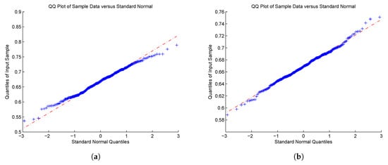
Figure 1. QQ-plot of ${\widehat{\varphi }}_K(1)$ for (CP); (a) $T_n=120$, and (b) $T_n=360$.

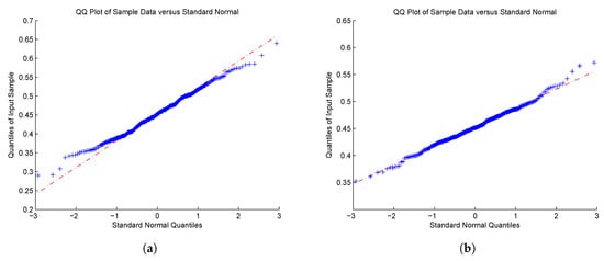
Figure 2. QQ-plot of ${\widehat{\varphi }}_K(3)$ for (CP); (a) $T_n=120$, and (b) $T_n=360$.

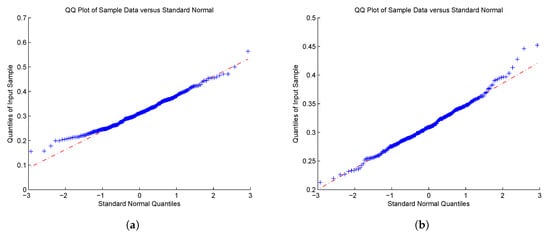
Figure 3. QQ-plot of ${\widehat{\varphi }}_K(5)$ for (CP); $T_n=120$ (a) and $T_n=360$ (b).

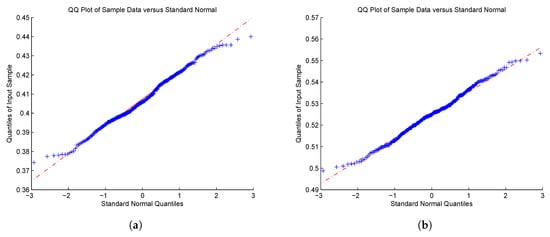
Figure 4. QQ-plot of ${\widehat{\varphi }}_K(1)$ for (GS); (a) $T_n=120$, and (b) $T_n=360$.

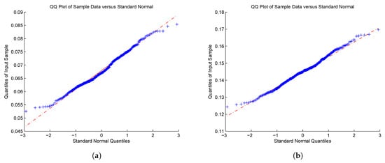
Figure 5. QQ-plot of ${\widehat{\varphi }}_K(3)$ for (GS); (a) $T_n=120$, and (b) $T_n=360$.

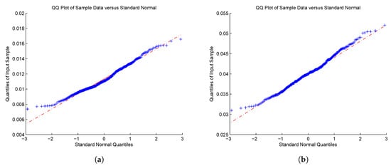
Figure 6. QQ-plot of ${\widehat{\varphi }}_K(5)$ for (GS); (a) $T_n=120$, and (b) $T_n=360$.

Most of the results manifest asymptotic normality as the value of $T_n$ becomes large. As for the case of ${\widehat{\varphi }}_K(5)$ with $T_n=360$ in Figure 3 and Figure 6, the right tails still seem not to converge to the normal distribution. Although we cannot explain this phenomenon quite well, it might be due to the value of ${ϵ}_n$ selected, which significantly affects the estimation of parameters. How to choose ${ϵ}_n$ in practice is an important problem, but this is beyond the scope of this paper. It is a theme that merits serious consideration by researchers.

6. Concluding Remarks

In this paper, we consider the statistical inference for ruin probability of Lévy insurance surplus under a certain sampling scheme. The samples consist of a mixture of n-discrete samples of the surplus, which are assumed to be a book record of the (e.g., daily) surplus, and a ‘large’ jumps that are insurance claims larger than a certain threshold ${ϵ}_n>0$.

We consider the Laguerre expansion of the ruin probability, which is the series expansion based on the Laguerre functions in (10) and the coefficients are obtained in explicit form that includes unknown quantities: the diffusion coefficient $D={\sigma }^2/2$ and functionals of Lévy measure of the form $\nu (H)={\int }_{\mathbb{R}}H(z)\nu (\mathrm{d}z)$. Those unknowns are estimable from our sampling data, and we showed the asymptotic properties of those estimators, which leads us the asymptotic normality of the estimated partial sum of Laguerre expansion of the ruin probability as $n\to \infty$ and ${ϵ}_n\to 0$ as well. The asymptotic distribution enables us to construct the asymptotic confidence intervals of ruin probability, which would be important to apply the ruin theory in practice.

In this paper, we assumed that ${ϵ}_n\to 0$ and that we can observe all the jumps that are larger than ${ϵ}_n$, which means that we can observe all the infinitely many jumps in the limit. Of course, such a situation is not realistic, but this paper investigates the rate of convergence and the possibility of the asymptotic normality of the estimators under a kind of ideal situation. We clarified the speed of ${ϵ}_n$ that goes to zero as in Proposition 9, which should be the first step to be specified in the theory of statistical inference. Note that the rate condition on ${ϵ}_n$ is only for theory, but is not checkable in practice as always in asymptotic statistics. In the simulation, we use ${ϵ}_n=2/T_n$ as an example that satisfies the asymptotic conditions in Proposition 9. However, in practice, the value of ${ϵ}_n$ is naturally determined, e.g., the value of deductible if it exists, or the smallest jump size within the observations. The asymptotics that ${ϵ}_n\to 0$ is a kind of approximation for the real situation: the theory ensures the statistical validity of our estimators if the value of ${ϵ}_n$ is practically ‘small’ enough and if we assume that the observed surplus is a realization of a Lévy process we assumed here. In this context, we may need “a new aspect" for the surplus model as described in Shimizu (2009).

7. Preliminary Lemmas

Lemma 3.

The functions $g_{\theta }$ and $h_{\theta }$ in Proposition 1 satisfy $g_{\theta },h_{\theta }\in L^1({\mathbb{R}}_{+})\cap L^2({\mathbb{R}}_{+})$.

Proof. 

Note that, from (1), it follows that

$${\pi }_{\infty }:={\int }_0^{\infty }\overline{\nu }(y),\mathrm{d}y={\int }_0^{\infty }\nu (\mathrm{d}z){\int }_0^z\mathrm{d}y={\int }_0^{\infty }z\nu (\mathrm{d}z)\in (0,\infty ).$$

Hence,

$$g_{\theta }(x)=\frac{c}{\theta }{\int }_0^x{e}^{-c(x-y)/\theta }\overline{\nu }(y)\mathrm{d}y\le \beta {\int }_0^{\infty }\overline{\nu }(y)\mathrm{d}y\le \beta {\pi }_{\infty }<\infty .$$

Moreover, note that ${\pi }_d(x)={\pi }_{\infty }^{-1}\overline{\nu }(x)$ is a probability density function, and $g_{\theta }(x){\pi }_{\infty }^{-1}c=k_{\theta }\ast {\pi }_d(x)$ is the probability density. In particular, we see that $g_{\theta }$ is the density of a defective distribution since

$$\begin{array}{c}\hfill {\int }_0^{\infty }{g}_{\theta }(x)\mathrm{d}x=\frac{{\pi }_{\infty }}{c}<1\end{array}$$

(25)

by (3). Therefore,

$${\int }_0^{\infty }{g}_{\theta }^2(x)\mathrm{d}x\le \beta {\pi }_{\infty }{\int }_0^{\infty }{g}_{\theta }(x)\mathrm{d}x<\beta {\pi }_{\infty }<\infty .$$

Note that

$${\pi }_{\infty }^{-1}\Lambda (x)={\int }_x^{\infty }{\pi }_d(y)\mathrm{d}y\le 1$$

since the last term is a probability tail function. Hence, $\Lambda (x)\le {\pi }_{\infty }$, which yields

$$\begin{array}{cc}\hfill \underset{x\in {\mathbb{R}}_{+}}{sup}\left|h(x)\right|& \le \frac{1}{b}{\int }_0^x\Lambda (x-y)k_{\theta }(y)\mathrm{d}y+1\hfill \\ & \le \frac{{\pi }_{\infty }}{c}{\int }_0^{\infty }{k}_{\theta }(x)\mathrm{d}x+1=\frac{{\pi }_{\infty }}{c}+1<\infty .\hfill \end{array}$$

As a consequence,

$$\begin{array}{cc}\hfill {\int }_0^{\infty }{h}^2(x)\mathrm{d}x& \le \left({\pi }_{\infty }{c}^{-1}+1\right){\int }_0^{\infty }h(x)\mathrm{d}x\hfill \\ & =\left({\pi }_{\infty }{c}^{-1}+1\right)\left({\int }_0^{\infty }{k}_{\theta }\ast \Lambda (x)\mathrm{d}x+{\beta }^{-1}\right)\hfill \\ & \le \left({\pi }_{\infty }{c}^{-1}+1\right)\left({\pi }_{\infty }+{\beta }^{-1}\right)<\infty .\hfill \end{array}$$

This completes the proof. □

Lemma 4.

$\varphi \in L^p({\mathbb{R}}_{+})$ for any $p\ge 1$.

Proof. 

From Proposition 1, we have the following Laplace transform of $\varphi$:

$${\int }_0^{\infty }{e}^{-sx}\varphi (x)\mathrm{d}x=\frac{{\int }_0^{\infty }{e}^{-sx}{h}_{\theta }(x)\mathrm{d}x}{1-{\int }_0^{\infty }{e}^{-sx}{g}_{\theta }(x)\mathrm{d}x}.$$

The last term of right-hand side can be attributed to $s=0$ since $g_{\theta },h_{\theta }\in L^1({\mathbb{R}}_{+})$ by Lemma 3. Therefore, we have

$${\int }_0^{\infty }\varphi (x)\mathrm{d}x=\frac{{\int }_0^{\infty }{h}_{\theta }(x)\mathrm{d}x}{1-{\int }_0^{\infty }{g}_{\theta }(x)\mathrm{d}x}<\infty .$$

Hence, $\varphi \in L^1({\mathbb{R}}_{+})$. Considering that $0\le \varphi (x)\le 1$ is the probability of ruin, it follows for any $p\ge 1$ that

$${\int }_0^{\infty }{\varphi }^p(x)\mathrm{d}x\le {\int }_0^{\infty }\varphi (x)\mathrm{d}x<\infty .$$

This completes the proof. □

Lemma 5.

Let $f:\mathbb{R}\to \mathbb{R}$ be a differentiable function such that $\left|f(x)\right|+|f^{\prime }{(x)|\lesssim 1+|x|}^C$ for a constant $C>0$, and let $k_{\lambda }(x)=\lambda e^{-\lambda x}(x\ge 0)$ for $\lambda >0$. It then follows that

$$\underset{\lambda \to \infty }{lim}{\int }_0^{\infty }{k}_{\lambda }(x)f(x)\mathrm{d}x=f(0).$$

Proof. 

Since f is a polynomial growth function, we see, using integration by parts, that

$$\begin{array}{c}\hfill {\int }_0^{\infty }{k}_{\lambda }(x)f(x)\mathrm{d}x=f(0)+{\int }_0^{\infty }{e}^{-\lambda x}{f}^{\prime }(x)\mathrm{d}x\end{array}$$

Taking a constant $\delta \in (0,\lambda )$, we have

$$|e^{-\lambda x}{f}^{\prime }(x)|=e^{-(\lambda -\delta )x}|e^{-\delta x}{f}^{\prime }(x)|\le |e^{-\delta x}{f}^{\prime }(x)|,$$

with the last function being integrable. Therefore, it follows from the Lebesgue convergence theorem that

$$\begin{array}{cc}\hfill \underset{\lambda \to \infty }{lim}{\int }_0^{\infty }{k}_{\lambda }(x)f(x)\mathrm{d}x& =f(0)+{\int }_0^{\infty }\underset{\lambda \to \infty }{lim}{e}^{-\lambda x}{f}^{\prime }(x)\mathrm{d}x=f(0).\hfill \end{array}$$

 □

References

- Biffis, Enrico, and Manuel Morales. 2010. On a generalization of the Gerber-Shiu function to path dependent penalties. Insurance: Mathematics and Economics 46: 92–97. [Google Scholar] [CrossRef]
- Carroll, Raymond J., Arnoud C. M. Van Rooij, and Frits H. Ruymgaart. 1991. Theoretical aspects of ill-posed problems in statistics. Acta Applicandae Mathematica 24: 133–40. [Google Scholar] [CrossRef]
- Chauveau, D. El, A. C. M. Vanrooij, and F. H. Ruymgaart. 1994. Regularized inversion of noisy Laplace transforms. Advances in Applied Mathematics 15: 186–201. [Google Scholar] [CrossRef]
- Feng, Runhuan, and Yasutaka Shimizu. 2013. On a generalization from ruin to default in a Lévy insurance risk model. Methodology and Computing in Applied Probability 15: 773–802. [Google Scholar] [CrossRef]
- Huzak, Miljenko, Mihael Perman, Hrvoje Šikić, and Zoran Vondraček. 2004. Ruin probabilities and decompositions for general perturbed risk processes. The Annals of Applied Probability 14: 1378–97. [Google Scholar]
- Jacod, Jean. 2007. Asymptotic properties of power variations of Lévy processes. ESAIM: Probability and Statistics 11: 173–96. [Google Scholar] [CrossRef]
- Kyprianou, Andreas E. 2014. Fluctuations of Lévy Processes with Applications. Introductory Lectures, 2nd ed.Heidelberg: Springer. [Google Scholar]
- Lundberg, Fillip. 1903. Approximerad Framställning av Sannolikehetsfunktionen. Ph.D. Dissertation, Aterförsäkering av Kollektivrisker, Almqvist & Wiksell, Stockholm, Uppsala. [Google Scholar]
- Mnatsakanov, Robert, L. L. Ruymgaart, and Frits H. Ruymgaart. 2008. Nonparametric estimation of ruin probabilities given a random sample of claims. Mathematical Methods of Statistic 17: 35–43. [Google Scholar] [CrossRef]
- Schoutens, Wim, and Jessica Cariboni. 2009. Lévy Processes in Credit Risk. New York: John Wiley & Sons Ltd. [Google Scholar]
- Shimizu, Yasutaka. 2009. A new aspect of a risk process and its statistical inference. Insurance: Mathematics and Economics 44: 70–77. [Google Scholar] [CrossRef]
- Shimizu, Yasutaka. 2011. Estimation of the expected discounted penalty function for Lévy insurance risks. Mathematical Methods of Statistics 20: 125–49. [Google Scholar] [CrossRef]
- Shimizu, Yasutaka. 2012. Nonparametric estimation of the Gerber-Shiu function for the Wiener-Poisson risk model. Scandinavian Actuarial Journal 2012: 56–69. [Google Scholar] [CrossRef]
- Shimizu, Yasutaka, and Shuji Tanaka. 2018. Dynamic risk measures for stochastic asset processes from ruin theory. Annals of Actuarial Science 12: 249–68. [Google Scholar] [CrossRef]
- Shimizu, Yasutaka, and Zhimin Zhang. 2017. Estimating Gerber-Shiu functions from discretely observed Lévy driven surplus. Insurance: Mathematics and Economics 74: 84–98. [Google Scholar] [CrossRef]
- Trufin, Julien, Hansjoerg Albrecher, and Michel M. Denuit. 2011. Properties of a risk measure derived from ruin theory. The Geneva Risk and Insurance Review 36: 174–88. [Google Scholar] [CrossRef]
- Zhang, Zhimin. 2016. Estimating the Gerber-Shiu function by Fourier-Sinc series expansion. Scandinavian Actuarial Journal 2017: 898–919. [Google Scholar] [CrossRef]
- Zhang, Zhimin, and Wen Su. 2017. A new efficient method for estimating the Gerber-Shiu function in the classical risk model. Scandinavian Actuarial Journal 5: 426–49. [Google Scholar] [CrossRef]
- Zhang, Zhimin, and Hailiang Yang. 2013. Nonparametric estimate of the ruin probability in a pure-jump Lévy risk model. Insurance: Mathematics and Economics 53: 24–35. [Google Scholar] [CrossRef]
© 2019 by the authors. Licensee MDPI, Basel, Switzerland. This article is an open access article distributed under the terms and conditions of the Creative Commons Attribution (CC BY) license (http://creativecommons.org/licenses/by/4.0/).