1. Introduction
Mortality contributes significantly to population dynamics and is crucial in many fields such as economy, demography and social sciences. Since the beginning of the nineteenth century, life expectancy has shown a continuous growth in developed countries (at a steady pace since the end of the Second World War), often at a more rapid rate than expected according to forecasts (
Oeppen and Vaupel (
2002)). This has created financial challenges for life insurers, pension plans and social security schemes involving benefits related to illness, death or survival of people. Mortality forecasting is then considered a key challenge for these entities.
Presently, refined techniques to forecast future mortality are becoming common among actuaries to treat longevity risk as well as to obtain more accurate prediction of life expectancy. In the context of extrapolative stochastic mortality models, the
Lee and Carter (
1992) model is the most frequently used, due to some advantages like the small number of parameters compared to other models and the robustness. The model’s parsimony results in a model in which mortality is stable with age, preventing the crossing of the age profile lines in the forecasting phase (see
Li et al. (
2009) for further details).
In recent years, thanks to the computational ability improvement, machine learning techniques are back on stage. Machine learning encloses many algorithms that learn from large datasets with many features and it is very useful in detecting unknown and unidentifiable patterns. Despite the increasing usage in different fields of research, machine learning applications are not so popular in demography, mainly due to the findings often considered as “black boxes” and then difficult to interpret. Moreover, machine learning algorithms are driven by data and not supported by specific hypotheses, to which demographers are more interested.
In spite of the reserve of demographers, research contributions in this field are increasing. We provide a reminder of
Hainaut (
2018), who proposes a neural network to predict and simulate mortality rates. The author uses a neural analyzer for identifying latent time processes and directly predicting mortality. This approach allows for detecting and duplicating nonlinearities observed in the evolution of log-forces of mortality.
Deprez et al. (
2017) use some machine learning techniques to improve the estimation of the log mortality rates, extended by
Levantesi and Pizzorusso (
2018) to the mortality forecasting in the Lee–Carter framework. Moreover, the recent paper of
Richman and Wüthrich (
2018) proposes a multiple-populations Lee–Carter model where parameters are estimated using neural networks. Other relevant applications of machine learning in an actuarial field can be found e.g., in
Castellani et al. (
2018) and
Gabrielli and Wüthrich (
2018).
In this paper, we use deep learning techniques in order to improve the predictive ability of the Lee–Carter model. Specifically, our approach aims to integrate the original Lee–Carter formulation introducing a Recurrent Neural Network with Long Short-Term Memory (LSTM) architecture to forecast future evolution of parameter, overcoming the limitation showed by the ARIMA processes. We think that the use of LSTM allows for obtaining mortality forecasts more coherent with the observed mortality dynamics, also in cases of nonlinear mortality trends. More precisely, the LTSM network is structured in order to elaborate long sequences of data, forming a memory able to preserve the significant relationships between data, also very distant in the sequence. In this sense, inside the time series context, LSTM allows for predicting future mortality over time considering the significant influence of the past mortality trend and adequately reproduces it into the forecasted trend. Then, strength of LSTM is then to preserve the information over time, thus preventing older signals from gradually vanishing during processing.
Therefore, the paper is focused on the forecasting of mortality trend, while the parameter estimation remains the same from
Lee and Carter (
1992). Specifically, we do not propose a new methodology for fitting the mortality surface (already introduced by
Hainaut (
2018) that uses neural networks for fitting mortality rates alternatively to the traditional singular value decomposition); instead, we introduce an innovative structure based on an LSTM network for modeling future mortality trends.
This paper is organized as follows.
Section 2 describes the traditional scheme of the Lee–Carter model,
Section 3 describes neural networks with particular attention to the LSTM networks.
Section 4 is dedicated to the numerical application carried out on a set of six countries throughout the world and
Section 5 provides conclusions.
3. Neural Network Model
The term neural network (NN) originated as a mathematical model that replicates the biological neural networks of the human brain (
Minsky and Pitts (
1943);
Wiener (
1948)). NN architecture includes neurons, synaptic connections that link the neurons, and learning algorithms. Typically, NN is formed by three types of layers, respectively, called input, hidden and output layer and each one has several neurons. Each unit in a network gets “weighted” information through synaptic links from the other connected ones and returns an output by using an activation function transforming the weighted sum of input signals.
Considering a single neuron
H—called perceptron by
Rosenblatt (
1958)—its output is defined as:
where
is the input,
is the associate synaptic weight,
is the number of input signals and
is the activation function. The term
represents the bias, also called activation threshold. It is important to notice that the function
must be differentiable because the learning equations are gradient-based.
NN with a single layer cannot be used for nonlinear separable problems like XOR (
Minsky and Papert (
2017)) but the introduction of MultiLayer Perceptron (MLP) has inspired new structures of more powerful NNs that overcome this limitation. In the MLP, the neurons are predisposed on different layers and each unit is fully-connected with those of the previous layer.
The way in which the units are connected by synapses defines different types of networks. In the NN classical pattern (feedforward NN), the information moves from the input to the output layer in only one direction, while, in the Recurrent Neural Networks (RNNs), the information is processed cyclically using additional synapses such that the result of the elaboration process was reprocessed as input.
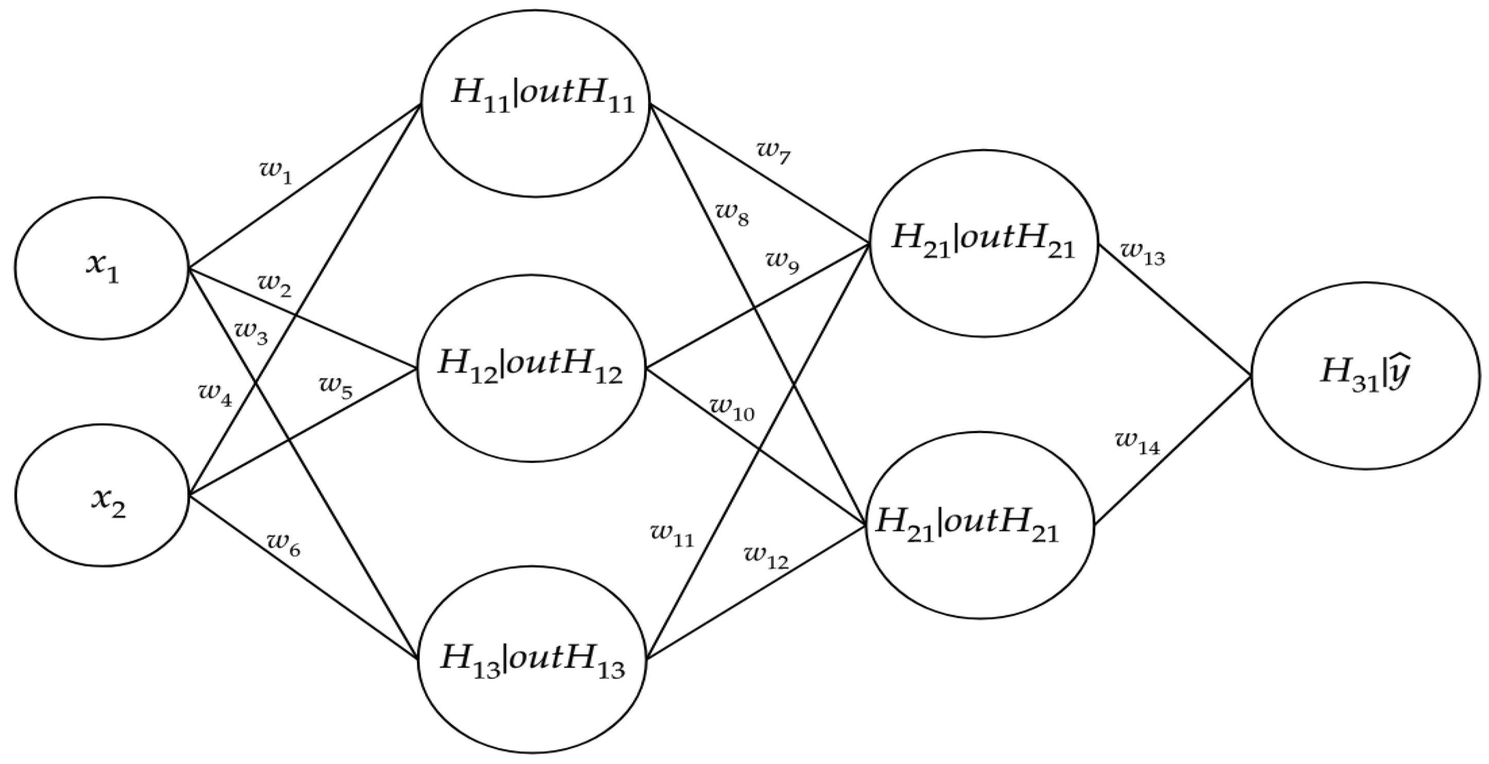
Figure 1 shows the typical feedforward NN representation. Every node of the graph represents a neuron, connected to each other by arcs representing the synapses. In the graph, the generic input, latent, and output variables are represented.
The output
of a generic hidden layer with
neurons is defined:
where
is a weight matrix and
is a biases vector. In the MLP scheme, the output of a hidden layer becomes the input for the next layer.
Considering a regression problem, where
is the number hidden layers, the output
is obtained by:
where
are weight matrices,
are bias vectors, and
are activation functions not necessarily different from each other. It is important to notice that the dimension of the weight matrices and the bias vectors depend on the number of units in the hidden layers. Increasing the number of hidden layers, the level of abstraction of the input data increases.
Back-propagation
NN training involves an unconstrained optimization problem where the aim is to minimize a function in high dimensional space. Let us define a loss function:
that measures the difference between the predicted values
and observed ones
y. The quantity
E depends on the matrices of the weights
1 that influence the values of
. The aim is to find the values of the synaptic weights that minimize the quantity
E.
Among many other algorithms, the back-propagation is the most used for the training of feedforward NNs. The algorithm compares the predicted values against the desired ones (objective) and modifies the synaptic weights by back-propagating the gradient of the loss function. Schematically, the procedure alternates forward and backward propagation steps:
in the forward step, the prediction are computed fixing the synaptic weights,
in the backward step, the weights are adjusted in order to reduce the error E of the network.
The NN iteratively performs forward and backward propagation and modifies the weights to find the combination that minimizes the loss function.
Analytically, the back-propagation algorithm updates the weights
in the last layer using the delta rule (
Bryson and Ho (
1969)), defined as:
where
r is the learning rate. For the other previous layers, we proceed using the chain derivation rule. The updating of the weights matrix
are computed:
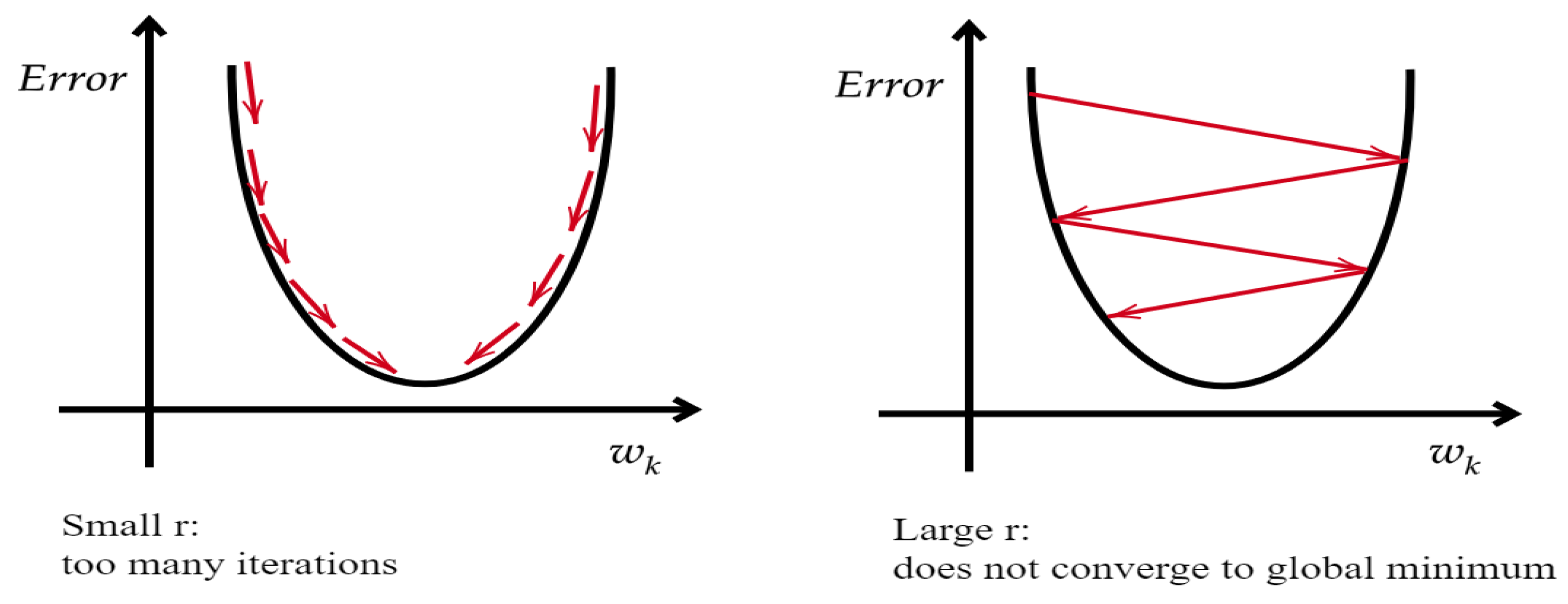
and so on for the other layers. In a figurative way, the idea behind the gradient descent is similar to “climbing down a hill” until a global or local minimum is reached. At each update, the search moves in the opposite direction of the gradient and the slope of the gradient and the learning rate determine the amplitude of this movement. In addition, the choice of the rate
r is an important element, since a small value involves too many iterations while a large value could not allow convergence to the global minimum.
Figure 2 shows the role of the learning rate in the convergence of the gradient descent in the simplest case of one-dimensional space.
The choices concerning the type of architecture (e.g., the number of hidden layers, units for each layer) and the hyperparameter values (e.g., learning rate, activation function, epochs) remain a heuristic problem for NN users: the choice often depends on the type of data and it is not an easy step. A preliminary round of hyperparameters tuning, before the testing, is highly desired. An extensive description of NNs and back-propagation algorithm can be found in
Alpaydin (
2010);
Hastie et al. (
2016) and
James et al. (
2017).
Recurrent Neural Network with Long Short-Term Memory Architecture
The feedforward NNs, although representing a powerful analysis tool (
Hornik et al. (
1989)), are inadequate to effectively manage time sequences of data.
The recurrent connections between nodes, which characterized the RNNs, allow for having a dynamic analysis of sequential data. However, by using the RNN structure, we usually face the major problem of gradients vanishing, in which the weights change, and becoming that small very fast as to have no effect. Therefore, the network gradually loses its ability to learn from the past, becoming operationally inadequate for the analysis of long data sequences and for making good predictions. For this reason, the RNNs have only a short memory.
To overcome this problem,
Hochreiter and Schmidhuber (
1997) developed the so-called Long Short-Term Memory, LSTM. The LSTM is an RNN whose architecture is such that it allows for considering the relationships between the data of the sequence, even if this is long, eliminating the vanishing gradient problem. In this manner, the RNNs acquire both long- and short-memory, managing to generate great performance, also in a time series context. After the original work, the LSTM has undergone several improvements, as shown in (
Gers et al. (
1999)) and (
Gers and Schmidhuber (
2000)), and it is now possible to define a well-composed basic structure called vanilla LSTM.
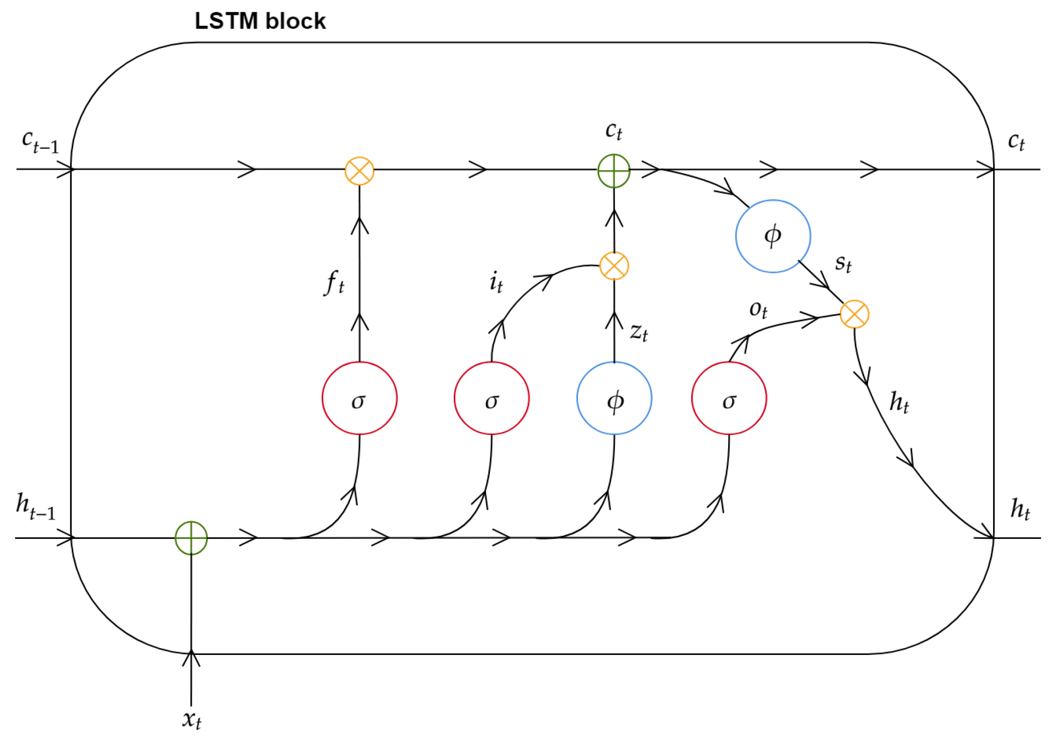
Accordingly with
Figure 3, the single LSTM unit, called LSTM block, is composed of three gates, their interactions and the resulting memory cell. The block receives as initial information flow the current input
, the previous short-term result
and the previous state of (long-term) memory cell
. The information is elaborated by three gates (red circle), named, respectively, forget gate, input gate and output gate, and auxiliary NNs (blue circle) helpful in the regularization of information flow.
Formally, referring to a hidden layer composed of
of LSTM blocks, letting
and
weight matrices (for each gate) be respectively associated to the input and to the previous short term result, the general mode of operation of a recurrent network with LSTM architecture is described by the following set of equations, specifying the forget gate output (
), input gate output (
), output of output gate (
), and output of auxiliary-output gate (
):
The forget gate output
, defined by Equation (
9), is such that the information from the previous cell state and the one coming from the current input are mixed in a nonlinear way by a sigmoid activation function. Therefore, the output can assume value between 0 and 1, forgetting or keeping the state of the previous block. Afterwards,
is mixed by a point-wise product with the previous state of memory
.
The input gate
, defined in Equation (
10), also uses a sigmoid activation, allowing for deciding when information received should be updated.
The output gate
, described in Equation (
11), has the role to prevent the transmission of non-significant memory content stored information to the other blocks. For this purpose, a sigmoid function is used in order to pass relevant memory information. In order to regularize the flow of processed data, the input gate
is combined with that obtained from the associated auxiliary NN
as in Equation (
12).
We define the processing of the entire input block, which participates in formulation of the current state of memory cell, as follows:
To obtain the current output, a combination between a function of
,
, and the upshot of auxiliary NN associated to output gate is necessary:
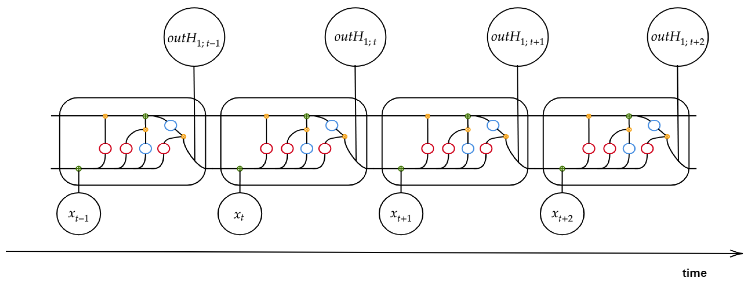
The output
is passed to the next layer and became the short memory
for the next instance. The general mode of RNN operation with LSTM architecture at each time step is represented in
Figure 4.
In light of the framework described above, we will show that the LSTM architecture is an excellent tool in the context of forecasting time series, especially in the case of very long time lag connections, as well as for catching and managing the noise. However, it is important to remind that the LSTM users, like those of NNs in general, have to face the classical problems concerning the choice of hyperparameters.
4. Numerical Application
In this section, we introduce the RNN with LSTM architecture in the classical scheme of the LC model. More precisely, our aim is to exploit the merits and functionalities of the LSTM architecture in order to improve the predictive capacity of the LC model. For this purpose, we design a set of experiments aimed to test the skills of LSTM in predicting the evolution of future mortality over time and to compare its performance with those derived from ARIMA.
Therefore, the analysis will concern the prediction of the time index
trend, considering the ARIMA model as forecast benchmark, while the parameters
and
are obtained according to the estimation procedure applied by
Lee and Carter (
1992).
Differently from the LC model that uses a random walk with drift, we calibrate the best ARIMA(p,d,q) according to the Hyndman–Khandakar algorithm (
Hyndman and Khandakar (
2008)). In the first round, the procedure checks the stationarity of the time series using an appropriate unit root test and chooses the differencing order
d. In a second stage, it selects the best values of auto-regressive and moving average order, respectively
p and
q, using a specific information criteria (AIC or BIC). The algorithm is implemented by the function
auto.arima available in the R package forecast (
Hyndman and Khandakar (
2008);
Hyndman et al. (
2019)).
The ARIMA performance is then compared to the LSTM one. The LSTM seems to be the more natural competitor of the ARIMA (p,d,q) model, for its ability to capture the long-term pattern inside the sequential data. We build a LSTM model that approximates the function
f linking
to its time lags, as follows:
where
is the number of time lags considered and
is a homoschedastic error term.
LSTM network, like other machine learning techniques, requires the splitting of the dataset into training set and testing set. The training set stands for supervised learning, while the testing is used to validate the model. The supervised learning dataset (
Table 1) is built as follows:
After the training phase, the network has learned the input–output functional relationship and it should be able to predict future values of using only the input. In practice, the input is a matrix of the time lags of and the output is the vector of its current values, where is the number of instances.
The forecasted values of , at time , are carried out recursively. In general terms, the predicted value of in a generic time is calculated using the values of with as input. It is important to note that, going forward in the forecasting, the future values of time index are calculated using only predicted values and not those observed. However, the forecasted data have not yet been observed, and the model’s accuracy becomes impossible to be measured.
The year T, which corresponds to the last observation in training set, is the starting point for forecasting. Therefore, we consider , where the observations before T represent the training set and the remaining form the testing set.
All experiments has been run with R version 3.5.2 (R Foundation for Statistical Computing, Vienna, Austria.
http://www.R-project.org/), using the keras, tensorflow, mlr (
Bischl et al. (
2016)), demography (
Hyndman (
2019)) and HMDHFDplus packages for the selected models. In addition, the package ggplot2 has been used for the results’ visualization.
The analysis is carried out on six countries, Australia, Denmark, Italy, Spain, the USA and Japan, and data are taken from the
Human Mortality Database (
2018). This database provides mortality rates, number of deaths and exposures for different ages and different countries distinguishing by gender. The whole period available in Human Mortality Database (HMD) has been considered for each country and the analysis has been performed considering one time lag (
).
The first step is to estimate the LC model parameters
,
and
using an SVD. The extracted time series of
represent the initial base for the analysis. These data are split into training and testing set according to the rule of 80% training and 20% testing. Therefore, the last year
T of observation is consequentially determined. The total available years and the corresponding testing set years considered in the analysis are shown in
Table 2 by country. The age range is set to 0–100.
In order to select the best combination of hyperparameters for the network, a preliminary round of fine-tuning is carried out for all countries, distinguishing by gender. The best combinations, obtained in this step, are used for the LSTM calibration in the forecasting procedure.
About the results of the tuning, we have noticed that the architectures with a single hidden layer work better than the others on our data and the number of neurons depends on the country. The Rectified Linear Unit (ReLU) activation function outperformed the other functions tested for all countries. In addition, no clear evidence emerged for the influence of other hyperparameters on the performance.
About the calibration of the ARIMA(p,d,q) model,
Table 3 shows the best specification for each country distinguished by gender.
Following the calibration step, the analysis includes numerical and graphical processing of the goodness of fit. In particular, we follow the out of sample approach that represents the testing step in the machine learning field. Concerning graphical analysis,
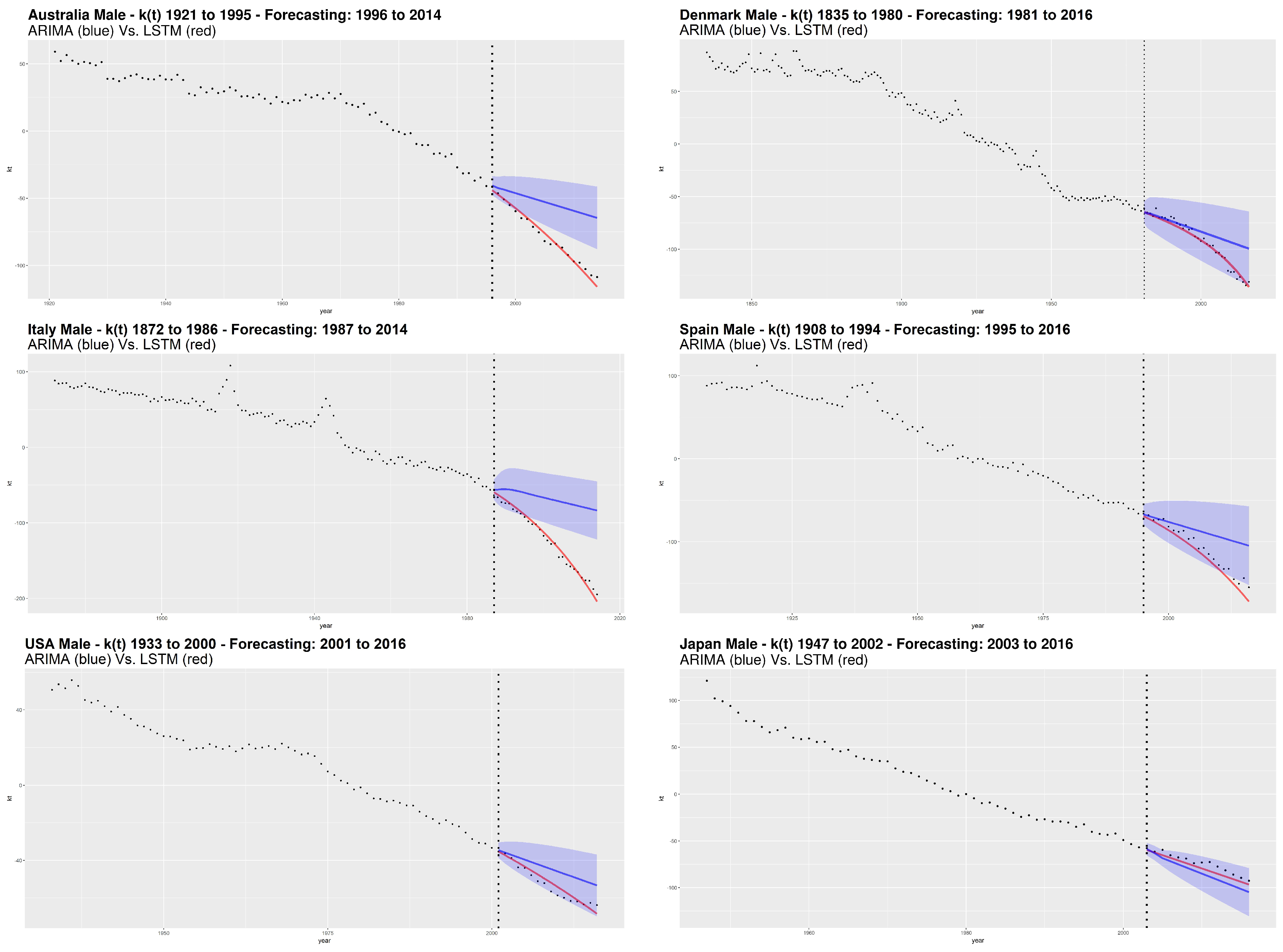
Figure 5 and
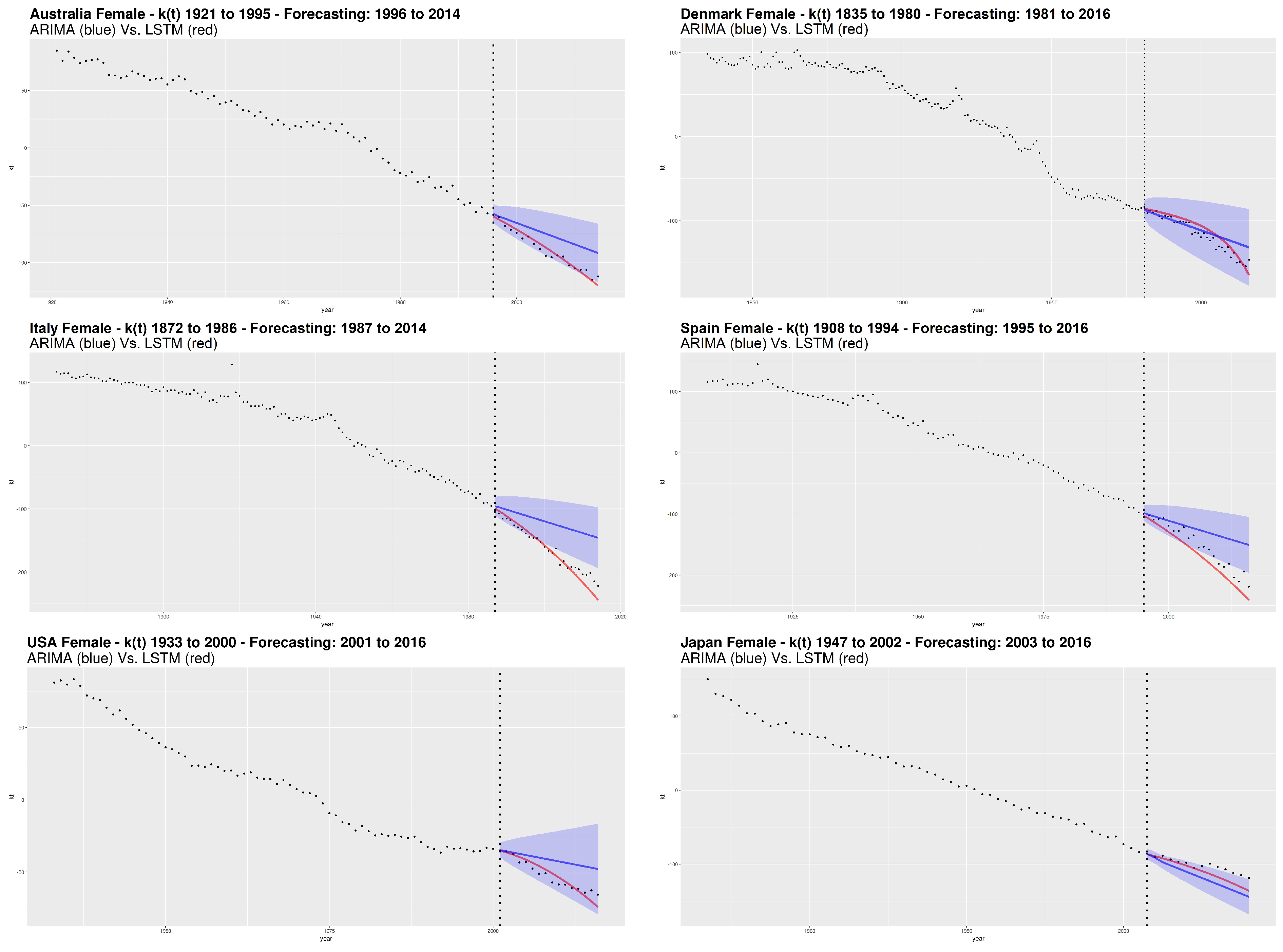
Figure 6 show the
parameter estimation obtained from SVD, respectively for male and female. The dashed vertical line separates the forecasted period from the one used to train the LSTM network. For the ARIMA models, we also show the confidence interval with
confidence level.
Besides graphical check, to compare the performance of LSTM against the best ARIMA in the testing set and measure the forecasting quality, we calculate the following goodness of fit measures:
Table 4 shows the performance of LSTM and ARIMA in terms of RMSE and MAE, by country and gender.
From the plots and the results of goodness of fit measures, we observe that the LSTM network provides the best performances compared to the ARIMA model.
Considering the error measures, MAE and RMSE, Italy shows the best LSTM performance with respect to the ARIMA for both genders. Also by a graphical analysis, the LSTM seems to catch very well the nonlinearity of the future mortality trend showing its remarkable ability to better represent the decreasing dynamics of mortality, with respect to the ARIMA model. The “worst” LSTM performance is obtained for Japan male and Denmark female, but still winning compared to the ARIMA.
More generally, we notice a higher capacity of the LSTM to capture nonlinear trends without incurring in the opposite situation, that is, an excessively oscillating or excessively parabolic trend (the latter observed in the traditional NNs). On the other hand, our analysis shows that ARIMA is not effective. The evolution of according to the ARIMA models is sometimes even outside of the confidence interval, like in the case of Italy (both genders), Australia (male) and Spain (female).
Our results highlight the inadequacy of ARIMA to detect the decreasing dynamics of mortality over time. Although the ARIMA process is widely used in modeling the time indexes of mortality, it has a fixed structure and works well when data satisfies the ARIMA assumptions, e.g., the constant variance assumption that is one of the most important features of the integrated models. In many cases, demographical data may exhibit volatility changes and this feature does not fit the ARIMA assumption, especially for long time series.
Although NN is a very powerful learning algorithm, it only provides point predictions without any indication of their variability. Confidence intervals prediction is a real challenge in the NN field. The literature on this topic is not extensive and the question is still open. Some scholars (
Khosravi et al. (
2011);
Keren et al. (
2019)) have faced this problem, but none of them has so far treated the question concerning NNs (and more generally deep learning) applied to time series. However, the LSTM network demonstrates being a good candidate to meet the need of predicting the mortality trend over time more accurately. We can state that LSTM overperforms the ARIMA model in all of the analyzed countries thanks to its architecture that allows for learning well the significant influence from the past mortality and replaces it with high precision for future years. This ability of LSTM network is noticeable, especially for populations where
parameter does not have a prominent linear trend.
Another remarkable aspect of LSTM concerns the possibility to achieve a good forecasting performance without resorting to a priori selection of the time steps. By way of example, we show the predicted values of life expectancy (
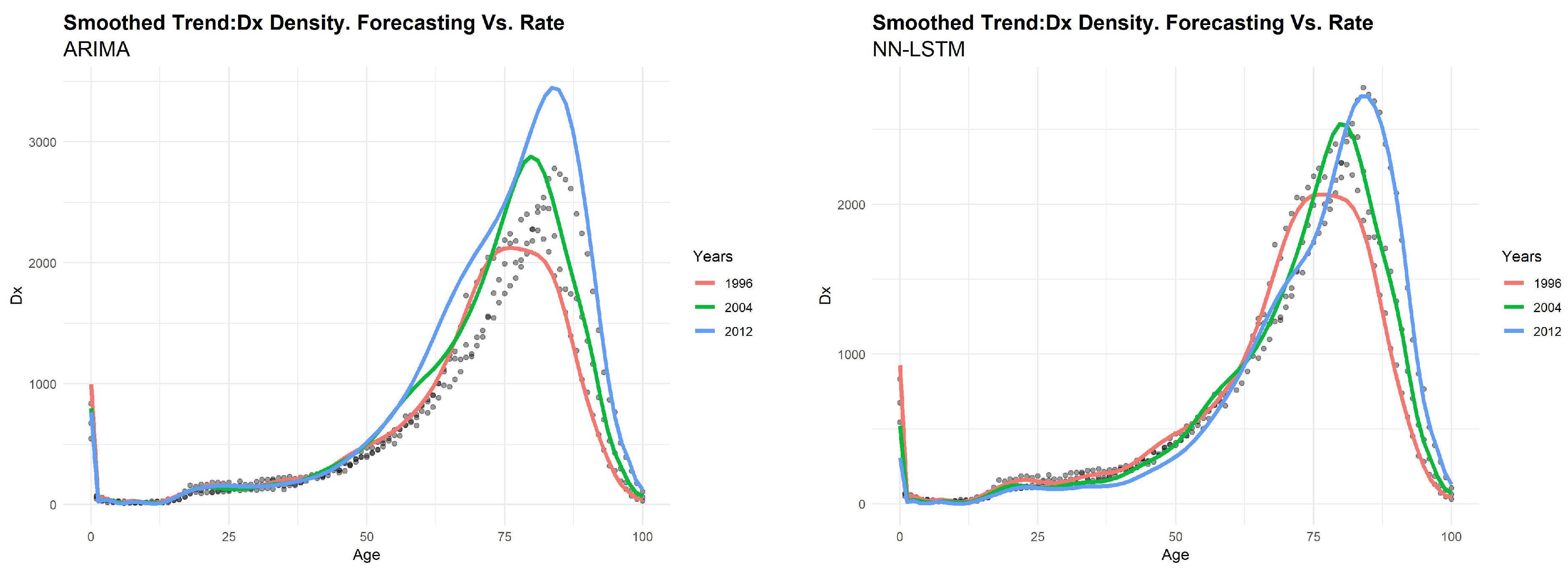
Figure 7), death distribution
(
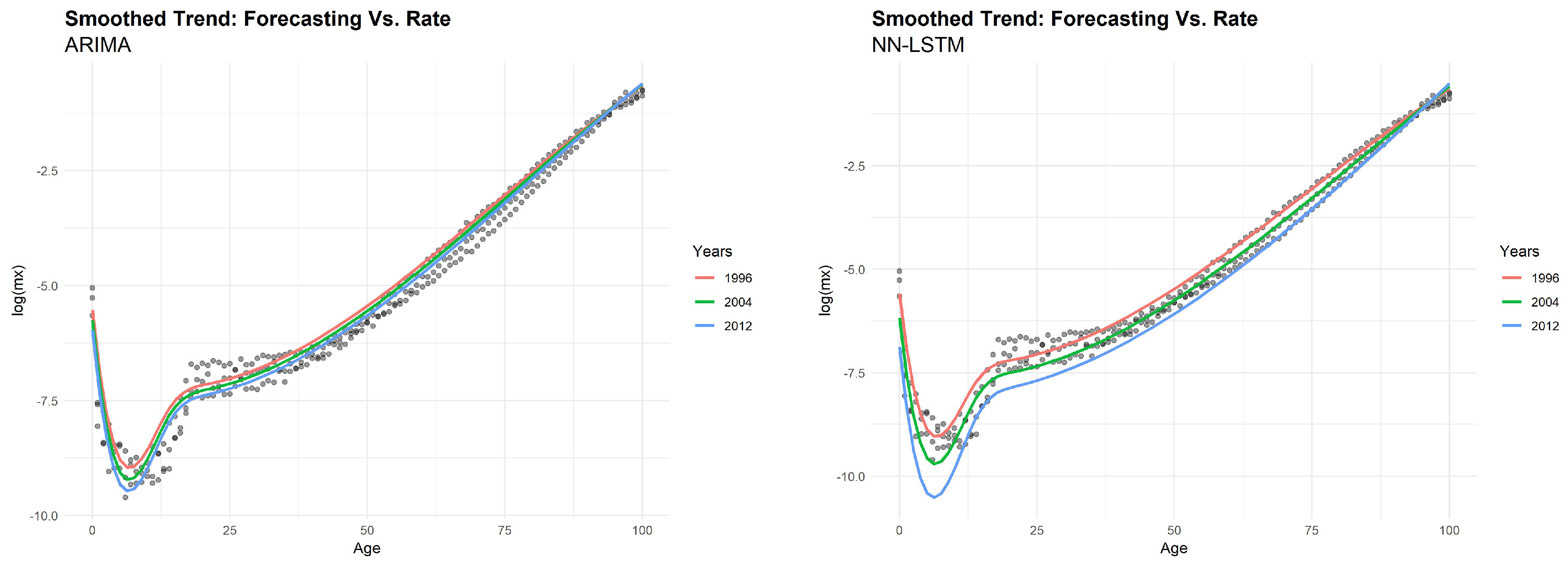
Figure 8) and log-mortality rates
(
Figure 9) obtained by both models for Australian males. All of the analyses presented here support the basic finding of an evident increase in life expectancy over time, as shown in the case of life expectancy at birth (
Figure 7, left side). The ARIMA model provides a trivial shape of forecasted trend. The straight line of future
values, constant over time, produces an unrealistic behavior of the forecasted mortality shape. Conversely, the LC model integrated with LSTM produces a negligible gap between the real and forecasted values of life expectancy. From the results of
and
depicted respectively in
Figure 8 and
Figure 9 using a smoothed shape, we can confirm that LSTM provides a better prediction on real data, respect to the ARIMA model.
5. Conclusions
In the mortality field, theories that embrace the steady increase in life expectancy have been extensively presented. In light of that, we can assert that mortality improvement is a fact. The shape of its pace remained a matter of debate. The latter point has an important reflection in the forecasting approach as well. For this reason, the field of nonlinear estimation of the time-dependent parameter in the LC model should represent a crucial point. Unfortunately, scholars have always focused efforts on enhancing LC fitting, overlooking a very important perspective: the forecasting trend.
In the present work, we have proposed a deep learning integrated LC model based on an RNN with LSTM architecture for the forecasting of the future values of index. The investigation has been performed on six countries throughout the world and by gender. The proposed approach shows very high accuracy levels of the mortality trend forecast, compared to the canonical ARIMA. Indeed, the LSTM stores excellent performance thanks to its architecture, consisting of three steps: catching, memorizing and replicating. These features allow the LSTM to provide more accurate forecasting, according to the decreasing trend of mortality over time, than the best ARIMA process.
Moreover, it can be noticed that the LSTM power is evident in the life expectancy trend and death distribution as well, in which, thanks to “out of sample” scheme, you can see the tangible impact on demographic forecasting of a new way of thinking that uses innovative forecast tools. The classical LC model, as well as other mortality models that use an ARIMA process, can produce a trivial shape of the forecasted trend, which provides a constant behavior of the forecasted mortality shape over time. The LSTM, catching a more realistic nonlinearity behavior, makes it possible to emphasize the differences between real and predicted values over time. In particular, concerning the life expectancy shape provided by the LC model integrated via LSTM, the discrepancy between the real value of the time series and the forecasted one is minimal. Our model provides a more optimistic scenario about mortality, in accordance with the widely accepted hypothesis of a constant increase in life expectancy.
This evidence supports the usefulness of the deep learning integration of the LC model proposed in the present work, which provides much more accurate predictions but at the same time preserves the LC advantages as parsimony and robustness. This last feature is particularly appreciated by the practitioners in life insurance industry, pension plans and social security schemes that have to compute and manage future cash flows, closely related to longevity dynamics. Since LSTM, and an NN in general, is a flexible tool, it is possible to overcome the ARIMA restrictions and conduct a more realistic evaluation. It is important to remember that the approach proposed in this paper provides point prediction, while the analysis of variability and the construction of confidence intervals remain an actual challenge in the NN field.
In a future work, we plan to extend the analysis to other countries included in the HMD database and explore the potentiality of the LSTM in other stochastic mortality models. In our opinion, the analysis of the variability and robustness of the LSTM (and machine learning models in general) remains one of the most important points in the field of data science and machine learning techniques (
Richman and Wüthrich (
2018)), which might be worth facing.
