On Double Value at Risk

Abstract

Value at Risk (VaR) is used to illustrate the maximum potential loss under a given confidence level, and is just a single indicator to evaluate risk ignoring any information about income. The present paper will generalize one-dimensional VaR to two-dimensional VaR with income-risk double indicators. We first construct a double-VaR with $(\mu ,{\sigma }^2)$ (or $(\mu ,Va{R}^2)$) indicators, and deduce the joint confidence region of $(\mu ,{\sigma }^2)$ (or $(\mu ,Va{R}^2)$) by virtue of the two-dimensional likelihood ratio method. Finally, an example to cover the empirical analysis of two double-VaR models is stated.

1. Introduction

In the early 1990s, the international economic and financial consultancy G30 published the report “derivatives practices and principles” based on the research on financial derivatives, and then proposed Value at Risk (VaR) model to measure the market risk. JP Morgan Bank then launched the VaR risk measurement and control model. Since VaR is accurate and comprehensive to the application of risk measurement and makes up the deficiency of Markowitz mean-variance model, it is generally welcomed by the international financial community, including regulatory authorities, and has become a standard to manage and control financial risk. Furthermore, VaR is widely used to measure credit risks and trading risks.

The biggest benefit of VaR is the ability to critically analyze risk through systematic analysis. The organization can control the front end and back end of the business by calculating VaR to understand the financial risks it faces and establish an independent risk management mechanism.

However, VaR also has its own limitations. Mausser and Rosen (1999) put forward the most obvious limitations of VaR: it does not provide absolute maximum loss value, which can only be expected in a certain confidence level. Another drawback of VaR is that when the calculation is based on historical data, the future situation of any event should be duplicated or fitted by historical data. However, the reality is that we cannot guarantee the future case of an event is just as old as. In addition, some researchers such as Artzner et al. (1999) criticized the VaR model because it does not meet sub-additivity.

The obvious limitation existing in VaR is that it is only used to illustrate the maximum possible loss for the given conditions and is only a single index to characterize the risk, which provides less information to users about other information such as income. In practice, what people usually care about is how much profit they can get while taking risks.

Based on the above considerations, we hope to follow the definition of VaR and Markowitz’s portfolio theory, and then construct a double-VaR, that is, we will extend one-dimensional single-risk monitoring indicator-VaR to two-dimensional revenue-risk monitoring indicators-VaR (or double-VaR for short).

There is abundant literature about VaR. Here, the main research literature involved in this paper is described briefly as follows.

Duffie and Pan (1997) made a detailed background description of VaR, characteristics, applications, and the entire VaR-system. Beder (1995) used eight different models to calculate VaR values and compare them. Some foreign scholars studied mainly the calculation of VaR, such as Jorion (1996); Linsmeier and Pearson (1996); Duffie and Pan (1997); Engle and Manganelli (1999). Based on different situations, they arrived at many calculation skills such as the variance-covariance matrix method, historical simulation, and Monte Carlo simulation method, and the related characteristics of VaR, etc.

After 1999, there are an increasing number of new VaR models in the financial, industrial, and other different applied areas. Potters and Bouchaud (1999) proposed how to use the normality of asset volatilities to calculate the VaR of nonlinear combination. Some other scholars studying the nature of VaR and other risk measurement methods, such as Artzner et al. (1999), proposed VaR does not meet sub-additivity; Wang (1999) studied the characteristics of dynamic risk measures; Mausser and Rosen (1999) proposed that if a small-probability event happened in the case of loss exceeding the VaR, then VaR models cannot measure the size of potential losses; Chen et al. (2014) studied future cash arbitrage with VaR-portfolio problems; Tang et al. (2018) investigated the no-arbitrage problem with VaR-like arguments; Cong and Zhao (2018; 2019) posed a non-cash risk measure and a generalized non-cash risk measure, respectively, which improved in some sense VaR under the distribution of any random variable that is uncertain. In addition, some scholars extended the classical Markowitz mean-variance model to the mean-VaR model; for instance, Pearson (2002) and Jorion (2007) used these models with constraints to manage the risk-profit for a fund company.

In addition, many scholars have proposed a series of improved calculation methods based on different markets and different assumptions. Berkowitz (1999) proposed a new method for evaluation of VaR. Taylor et al. (2000) proposed to use the t distribution to fit the income sequence; Hu (2012) based their research on the mixed Copula model to study the evaluation value of VaR; Ze-To (2013) used the Heath-Jarrow-Morton model to measure the value of VaR, and pointed out that the model can capture the non-normal income distribution well and can accurately provide the value of VaR; Li et al. (2017) confirmed that using the Bootstrap method to calculate VaR and CVaR can effectively improve the estimation accuracy.

Meanwhile, many foreign scholars have also attached great importance to the empirical applications of VaR. Jackson et al. (1997) studied how to apply VaR into bank reserves. Berkowitz and O’Brien (2002) proposed how to evaluate the transaction risk of commercial banks through the prediction accuracy of the VaR model. Basak and Shapiro (2001) analyzed the optimal dynamic portfolio risks with VaR model.

In the present paper, we will extend one-dimensional single-risk monitoring indicator—VaR—to two-dimensional benefit-risk monitoring indicators—double-VaR.

Firstly, a reasonable definition of two-dimensional VaR (double-VaR) is given. For a better understanding of double-VaR we choose mean $\mu$ and variance $\sigma$ as the parameters to build the first double-VaR model. Thus, for a given confidence level $\alpha$, one can not only know the scope of asset risks but also can know their income range. Such indicators are better able to make trade-offs to the risk-return of assets.

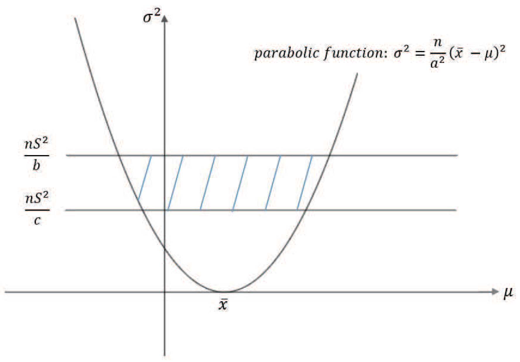
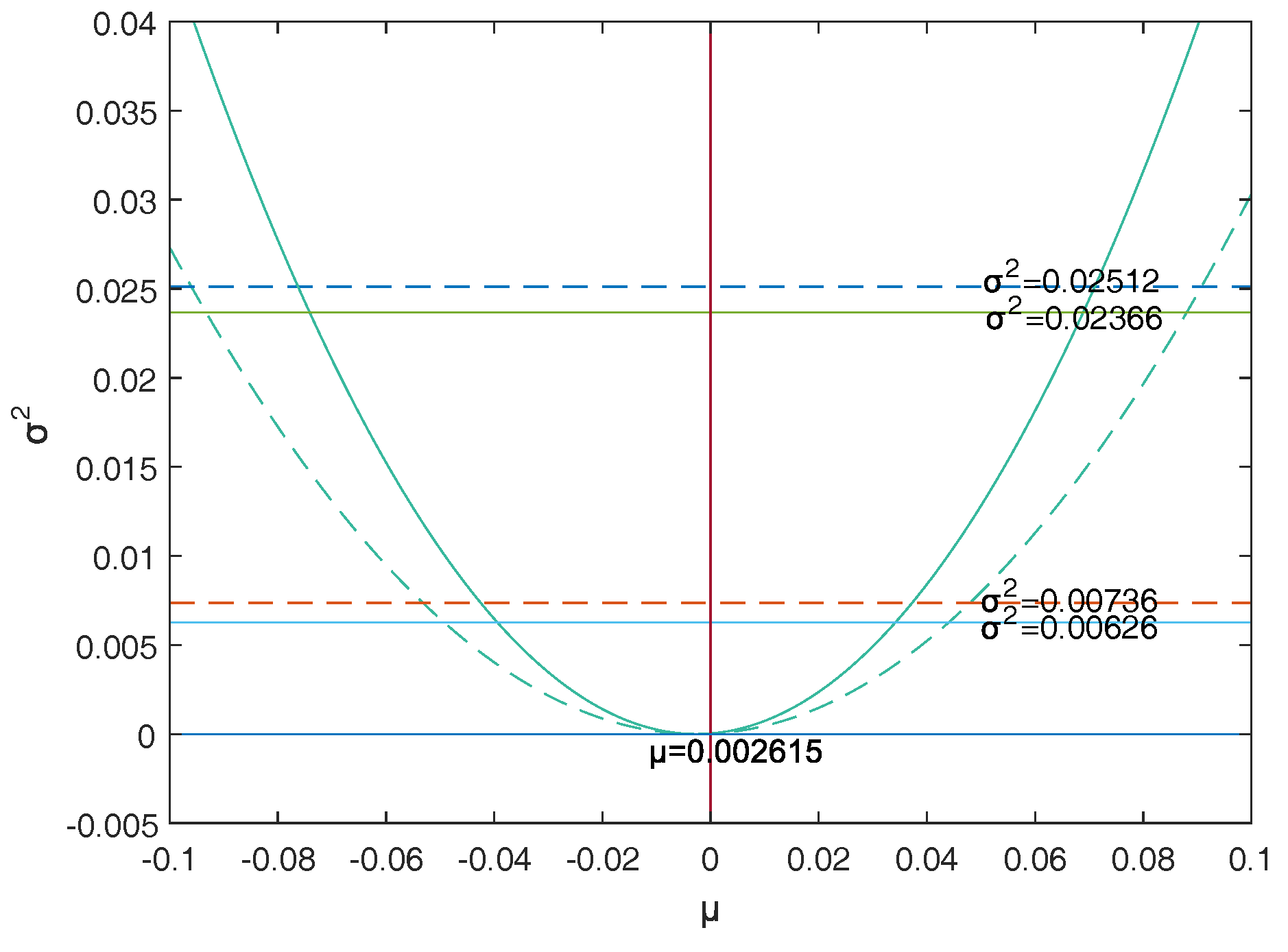
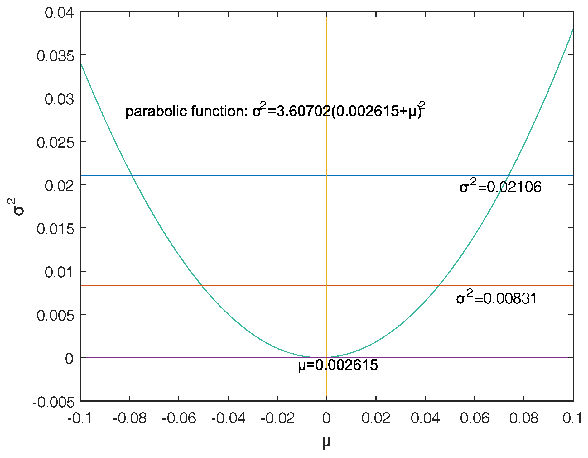
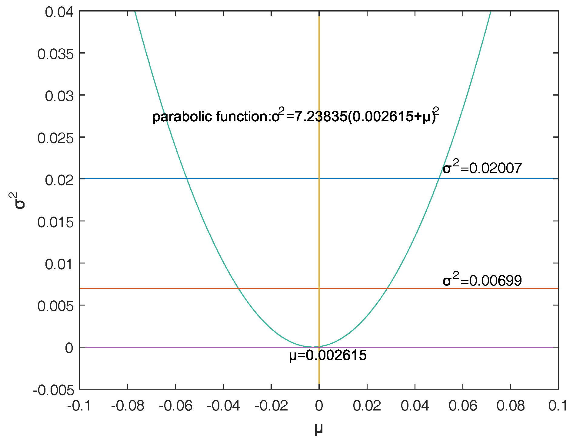
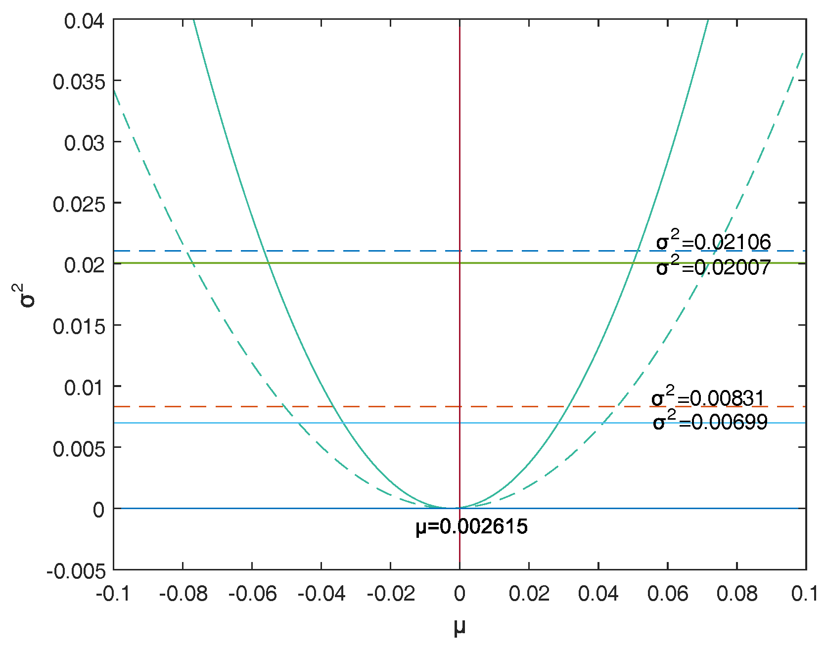
Secondly, to solve the first model—double-VaR with respect to $(\mu ,{\sigma }^2)$—we extend the one-dimensional likelihood ratio method to two-dimensional likelihood ratio method, and derive the joint confidence region containing the unknown parameters. Then, we can solve a specific joint confidence region with ideal point method and area minimization method as well as to compare the results of these two methods.

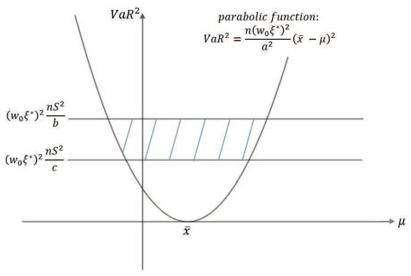
Finally, according to the accuracy theory of VaR we study the double-VaR based on $(\mu ,Va{R}^2)$ so that for a given confidence interval we cannot only know the biggest value of possible asset loss but we can also get the gain range. In this situation a better trade-off of the asset is possible.

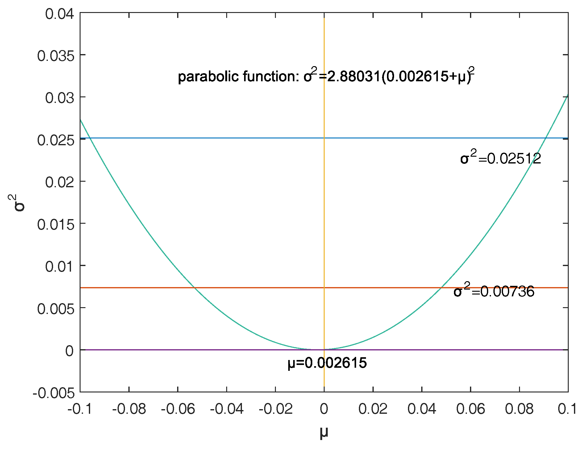
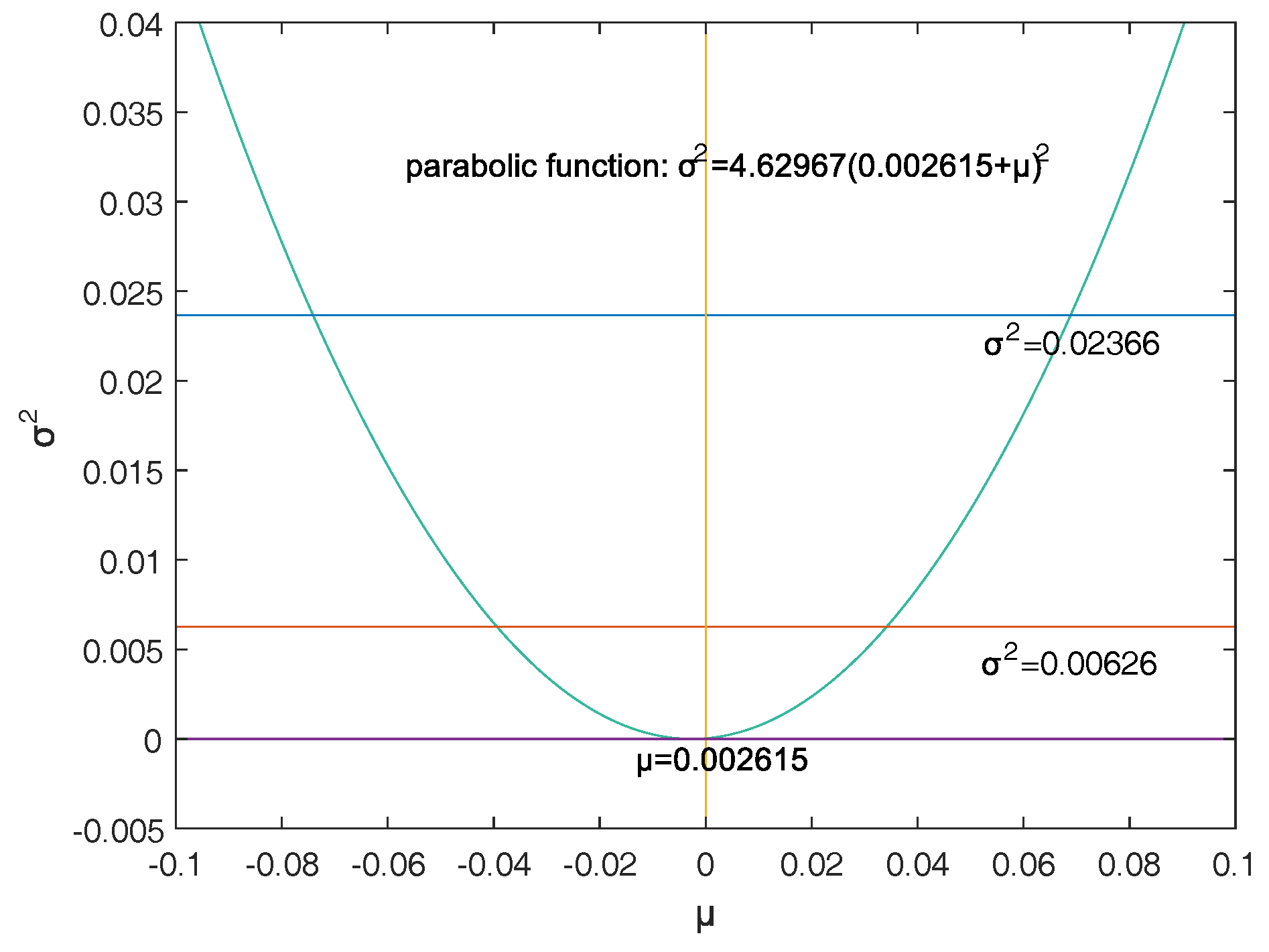
The organization of the paper is as follows. Section 2 introduces some necessary conditions and terminologies. Section 3 is devoted to constructing double-VaR models with $(\mu ,{\sigma }^2)$ and $(\mu ,Va{R}^2)$. Section 4 confirms that the double-VaR models are effective via some examples.

2. Preliminaries

2.1. VaR

2.1.1. Definitions and Basic Descriptions

Definition 1.

The basic meaning of VaR is the maximum potential loss of risk assets under normal market conditions, for a given confidence level α and holding period t. One can describe it as follows

$$P(\Delta p>VaR)=\alpha$$

where $\Delta p$ is the loss of risk asset W within the holding period t and VaR is the value at risk under the confidence level α.

Remark 1.

Under a normal market environment and a given confidence level α, let the probability distribution density function of a risky asset value be $f(w)$, the initial value of a risky asset be $w_0$, the lowest value of a risky asset under a confidence level α be $w^{*}$ and the yield on holding period t be r, then we have

$$VaR=E[w]-w^{*}$$

(1)

where $w=w_0(1+r)$ and $w^{*}$ can be achieved with the following two formulas

$$\alpha ={\int }_{w^{*}}^{\infty }f(w)dwor1-\alpha ={\int }_{-\infty }^{w^{*}}f(w)dw$$

(2)

In particular, when the distribution of the risk asset yield r is a normal distribution, that is, $r\sim N(\mu ,{\sigma }^2)$, then one can get VaR of the risk asset by the following steps:

Let

$$1-\alpha ={\int }_{-\infty }^{-{\xi }^{*}}\varphi (ϵ)dϵ$$

(3)

where $\varphi$ is the probability density function of a standard normal distribution. According to (2) and (3), we can get

$${\int }_{-\infty }^{-{\xi }^{*}}\varphi (ϵ)dϵ={\int }_{-\infty }^{w^{*}}f(w)dw={\int }_{-\infty }^{r^{*}}g(r)dr$$

(4)

where $g(r)$ is the normal probability density function of the risk asset with yield r. Since one has

$${\int }_{-\infty }^{-{\xi }^{*}}\varphi (ϵ)dϵ={\int }_{-\infty }^{w^{*}}\frac{1}{\sqrt{2\pi }}{e}^{-\frac{{ϵ}^2}{2}}dϵ$$

(5)

and

$${\int }_{-\infty }^{r^{*}}g(r)dr={\int }_{-\infty }^{r^{*}}\frac{1}{\sqrt{2\pi }\sigma }{e}^{-\frac{{(r-\mu )}^2}{2{\sigma }^2}}dr={\int }_{-\infty }^{\frac{r^{*}-\mu }{\sigma }}\frac{1}{\sqrt{2\pi }}{e}^{-\frac{1}{2}{t}^2}dt$$

(6)

where $t=\frac{r-\mu }{\sigma }$ and $t\sim N(0,1)$. We arrive here by (4) and (5)

$$r^{*}=\mu -\sigma {\xi }^{*}$$

(7)

Substitute (7) into (1), we then have

$$VaR=E[w]-w^{*}=w_0+w_{0}E[r]-(w_0+w_0{r}^{*})=w_0\sigma {\xi }^{*}$$

that is, there holds

$$VaR=w_0\sigma {\xi }^{*}$$

(8)

More generally, if one considers the time factor for VaR, then the Formula (8) can be written as $VaR=w_0\sigma {\xi }^{*}\sqrt{\Delta t}$.

In other words, when the yield on a risk asset follows a normal distribution, VaR measure of the risk is equivalent to the variance measure.

2.1.2. Properties of VaR

VaR has the following properties:

(1) Transformation invariance

For any $c\in \mathbb{R}$ and positive x, there holds $VaR(x+c)=VaR(x)+c.$

(2) Positive homogeneity

For any $c>0$, there holds $VaR(cx)=cVaR(x).$

(3) Co-monotonic additivity

For any $x,y$ is co-monotonic, there holds $VaR(x+y)=VaR(x)+VaR(y).$

(4) First-order stochastic dominance

For $x,y$, if the first order of x is better than that of y, there holds $VaR(x_1)\le VaR(x_2).$

(5) Discontinuity on the confidence level

With respect to the confidence level $1-\alpha$, VaR is not continuous.

(6) Convexity is not satisfied

This property means that the local minimizer of an optimizing problem with VaR as an objective function is not unique.

(7) Sub-additivity is not satisfied

This means that VaR for a portfolio is not less than the sum of VaR of all risky assets.

3. Double-VaR

3.1. Introduction of Double-VaR

We now chose the mean and variance as two proposed parameters-based on Markowitz’s portfolio theory to form a revenue-risk region D. Then we can define VaR-like as follows

$$P\{(\mu ,{\sigma }^2)\in D\}=1-\alpha$$

Remark 2.

It is not hard to speculate that the role of the revenue-risk region D in fact is similar to that of VaR. For convenience, we may call the boundary (or partial boundary) of D a double-VaR with respect to indexes μ and ${\sigma }^2$. A detailed definition of double-VaR will be given later.

Its real economic significance is under the normal market environment and a given confidence level, an area in which the maximum possible loss (expressed by var ${\sigma }^2$) and the benefits (expressed by mean μ) of an asset within a certain time in the future falls.

3.2. Double-VaR Model with Respect to $(\mu ,{\sigma }^2)$

3.2.1. Two-Dimensional Likelihood Ratio Argument

Chen and Jiang (2017) proposed and studied a high-dimensional likelihood method for normal distribution. However, for the use of the two-dimensional likelihood method for the derivation of the joint confidence domain, we have not found relevant literature. Thus, we innovate based on learning their ideas to solve the two-dimensional joint confidence region for double-VaR problem.

Assume that the total distribution of $\xi$ follows a distribution whose density function is $f(x;\theta )$, where the parameters $\theta =({\theta }_1,{\theta }_2)$ are unknown. For the given sample observations, it is easy to get the likelihood function:

$$L({\theta }_1,{\theta }_2)=L(x_1,x_2,\cdots ,x_n;{\theta }_1,{\theta }_2)=\prod _{i=1}^{n}f(x_i;\theta ).$$

If the maximum likelihood estimation of $({\theta }_1,{\theta }_2)$ is $({\widehat{\theta }}_1,{\widehat{\theta }}_2)$ that is, $L({\widehat{\theta }}_1,{\widehat{\theta }}_2)=\underset{\theta \in \mathrm{\Theta }}{sup}({\theta }_1,{\theta }_2)$, $\mathrm{\Theta }$ is the parameter space of $\theta$, the likelihood ratio can be defined as

$$R=R(x_1,x_2,\cdots ,x_n;{\theta }_1,{\theta }_2)=\frac{L({\theta }_1,{\theta }_2)}{L({\widehat{\theta }}_1,{\widehat{\theta }}_2)}.$$

For a given confidence level, the joint confidence region D of the parameter $\theta =({\theta }_1,{\theta }_2)$ can be calculated by R.

When the total $\xi \sim N(\mu ,{\sigma }^2)$, where $(x_1,x_2,\cdots ,x_n)$ is a set of sample values and the confidence level is $1-\alpha$, the joint confidence region of $(\mu ,{\sigma }^2)$ can be gained by the following two-dimensional likelihood ratio, where the unknown parameter is $\theta =(\mu ,{\sigma }^2)$.

In fact, we have known the maximum likelihood estimations of mean $\mu$ and variance ${\sigma }^2$ are respectively by $\widehat{\mu }=\overline{x}$ and ${\widehat{\sigma }}^2=s^2=\frac{1}{n}{\displaystyle \sum _{i=1}^n}{(x_i-\overline{x})}^2$. Then we get

$$L(\mu ,{\sigma }^2)={(2\pi {\sigma }^2)}^{-\frac{n}{2}}exp\left\{-\frac{1}{2{\sigma }^2}\sum _{i=1}^n{(x_i-\mu )}^2\right\},$$

$$L(\widehat{\mu },{\widehat{\sigma }}^2)={(2\pi s^2)}^{-\frac{n}{2}}exp\left\{-\frac{1}{2s^2}\sum _{i=1}^n{(x_i-\overline{x})}^2\right\}.$$

Next we can get the likelihood ratio

$$R=\frac{L({\theta }_1,{\theta }_2)}{L({\widehat{\theta }}_1,{\widehat{\theta }}_2)}={\left(\frac{s^2}{{\sigma }^2}\right)}^{\frac{n}{2}}exp\left\{-\frac{1}{2{\sigma }^2}\sum _{i=1}^n{(x_i-\mu )}^2+\frac{1}{2s^2}\sum _{i=1}^n{(x_i-\overline{x})}^2\right\}$$

(9)

Since

$$\sum _{i=1}^n{(x_i-\mu )}^2=\sum _{i=1}^n{x}_i^2+n{\mu }^2-2\mu \sum _{i=1}^n{x}_i=\sum _{i=1}^n{x}_i^2+n{\mu }^2-2n\mu \overline{x}=\sum _{i=1}^n{x}_i^2-n{\overline{x}}^2+n{(\overline{x}-\mu )}^2.$$

Denote by $\frac{\overline{x}-\mu }{\sigma /\sqrt{n}}\widehat{=}M$ and $\frac{n{s}^2}{{\sigma }^2}\widehat{=}T$, thus we get the following

$$-\frac{1}{2{\sigma }^2}\sum _{i=1}^n{(x_i-\mu )}^2=-\frac{1}{2{\sigma }^2}\sum _{i=1}^n(x_i^2-n{\overline{x}}^2)-\frac{n}{2{\sigma }^2}{(\overline{x}-\mu )}^2=-\frac{1}{2{\sigma }^2}\sum _{i=1}^n(x_i^2-n{\overline{x}}^2)-\frac{1}{2}{M}^2.$$

Substitute the formula above into (9) and get

$$\begin{array}{cc}\hfill R& ={\left(\frac{T}{n}\right)}^{\frac{n}{2}}exp\left\{-\frac{1}{2{\sigma }^2}\sum _{i=1}^n(x_i^2-n{\overline{x}}^2)-\frac{1}{2}{M}^2+\frac{n}{2}\right\}\hfill \\ & ={\left(\frac{T}{n}\right)}^{\frac{n}{2}}\left\{-\frac{{\displaystyle \sum _{i=1}^n}(x_i^2-n{\overline{x}}^2)T}{2n{s}^2}-\frac{1}{2}{M}^2+\frac{n}{2}\right\}\hfill \\ & ={\left(\frac{T}{n}\right)}^{\frac{n}{2}}exp\left\{-\frac{1}{2}T-\frac{1}{2}{M}^2+\frac{n}{2}\right\}\hfill \end{array}$$

Since

$$\frac{\partial R}{\partial T}=n^{-\frac{n}{2}}\left(\frac{n}{2}{T}^{\frac{n}{2}-1}-\frac{1}{2}{T}^{\frac{n}{2}}\right)exp\left\{-\frac{1}{2}T-\frac{1}{2}{M}^2+\frac{n}{2}\right\},$$

and $T\ne 0$, if we let $\frac{\partial R}{\partial T}=0$, then there holds $T_0=n$. Since

$$\frac{\partial R}{\partial M}={\left(\frac{T}{n}\right)}^{\frac{n}{2}}(-M)exp\left\{-\frac{1}{2}T-\frac{1}{2}{M}^2+\frac{n}{2}\right\},$$

and $M\ne 0$. Let $\frac{\partial R}{\partial M}=0$, we arrive at $M_0=0$. For convenience, we denote by

$$\begin{array}{cc}\hfill A& \widehat{=}\frac{{\partial }^{2}R}{{\partial }^{2}M}{|}_{(M_0,T_0)}={\left(\frac{T}{n}\right)}^{\frac{n}{2}}(M^2-1)exp\left\{-\frac{1}{2}T-\frac{1}{2}{M}^2+\frac{n}{2}\right\}=-1,\hfill \\ \hfill B& \widehat{=}\frac{{\partial }^{2}R}{\partial T\partial M}{|}_{(M_0,T_0)}=n^{-\frac{n}{2}}\left(\frac{n}{2}{T}^{\frac{n}{2}-1}-\frac{1}{2}{T}^{\frac{n}{2}}\right)(-M)exp\left\{-\frac{1}{2}T-\frac{1}{2}{M}^2+\frac{n}{2}\right\}=0,\hfill \\ \hfill C& \widehat{=}\frac{{\partial }^{2}R}{{\partial }^{2}T}{|}_{(M_0,T_0)}=n^{-\frac{n}{2}}exp\left\{-\frac{1}{2}T-\frac{1}{2}{M}^2+\frac{n}{2}\right\}[\left(\frac{n}{2}{T}^{\frac{n}{2}-1}-\frac{1}{2}{T}^{\frac{n}{2}}\right)(-\frac{1}{2})\hfill \\ & +\frac{n}{2}(\frac{n}{2}-1)T^{\frac{n}{2}-2}-\frac{n}{4}{T}^{\frac{n}{2}-1}]=-\frac{1}{2n}.\hfill \end{array}$$

It is obvious that there holds

$$AC-B^2=\frac{1}{2n}-0>0.$$

By a sufficient condition of two-dimensional extreme points, we can know R has a strict maximum at the point $(M_0,T_0)$. Thus, for the constant C, there exists a region D so that $P\{R\ge C\}=P\{(M,T)\in D\}$. According to the meaning of likelihood ratio, let $P\{R\ge C\}=1-\alpha$, then $P\{(M,T)\in D\}=1-\alpha$. Since

$$M\sim N(0,1),T\sim {\chi }_{n-1}^2,$$

there exist three positive constants $a,b$ and $c(b<c)$, so that

$$P\{(M,T)\in D\}=P\{|M|\le a,b\le T\le c\}=P\left\{\left|\frac{\overline{x}-\mu }{\sigma /\sqrt{n}}\right|\le a,b\le \frac{n{s}^2}{{\sigma }^2}\le c\right\}=1-\alpha .$$

Since two statistics $M,T$ are $i.i.d$, there holds

$$P\left\{\left|\frac{\overline{x}-\mu }{\sigma /\sqrt{n}}\right|\le a,b\le \frac{n{s}^2}{{\sigma }^2}\le c\right\}=P\left\{\left|\frac{\overline{x}-\mu }{\sigma /\sqrt{n}}\right|\le a\right\}·P\left\{b\le \frac{n{s}^2}{{\sigma }^2}\le c\right\}=1-\alpha$$

(10)

That is

$$(2\mathrm{\Phi }(a)-1)({\chi }_{n-1}^2(c)-{\chi }_{n-1}^2(b))=1-\alpha ,$$

where ${\chi }_{n-1}^2(b)$ is the function value of ${\chi }_{n-1}^2$ distribution whose freedom is $n-1$ at the point b. Arrange (10) and get the joint confidence region of $(\mu ,{\sigma }^2)$ as below

$$\left\{(\mu ,{\sigma }^2):\overline{x}-\frac{a\sigma }{\sqrt{n}}\le \mu \le \overline{x}+\frac{a\sigma }{\sqrt{n}},\frac{n{s}^2}{c}\le {\sigma }^2\le \frac{n{s}^2}{b}\right\}$$

(11)

Obviously, there are unknowns a, b, and c in the joint confidence domain under the confidence level required by this paper. Therefore, to find these three unknowns, we can determine the specific joint confidence domain after given n and sample variance.

Definition 2.

Assume that $X\in {\mathbb{R}}^n$ is a random vector, and $(\mu ,{\sigma }^2)$ are two index parameters, for given confidence level $\alpha (0\le \alpha \le 1)$, one can define double-VaR of $X\in {\mathbb{R}}^n$ with respect to indexes $(\mu ,{\sigma }^2)$ as

$$Va{R}_{(\mu ,{\sigma }^2)}^{\alpha }(X)\widehat{=}\partial \left\{(\mu ,{\sigma }^2):\overline{x}-\frac{a\sigma }{\sqrt{n}}\le \mu \le \overline{x}+\frac{a\sigma }{\sqrt{n}},\frac{n{s}^2}{c}\le {\sigma }^2\le \frac{n{s}^2}{b}\right\}.$$

In the above definition, a, b, c are unknown. However, in Section 3.2.2, we use the ideal method to find the joint confidence domain. Thus, the unknown parameters a, b, c are solved. We can look up Table 1 and Table 2 to find the value of a, b, c.

Table 1. Ideal point method (confidence level is 99% and 95%).

	Ideal Point (Confidence Level: 99%)				Ideal Point (Confidence Level: 95%)
n	a	b	c	zz	a	b	c	zz
31	3.6185	13.0228	52.5124	0.0675	3.2248	15.9692	45.8943	0.0402
32	3.6284	13.6810	53.8337	0.0625	3.2340	16.7118	47.1456	0.0373
33	3.6373	14.3476	55.1539	0.0580	3.2427	17.4595	48.3940	0.0348
34	3.6454	15.0216	56.4719	0.0540	3.2510	18.2119	49.6392	0.0325
35	3.6529	15.7018	57.7869	0.0504	3.2590	18.9685	50.8812	0.0305
36	3.6601	16.3877	59.0984	0.0471	3.2666	19.7289	52.1197	0.0286
37	3.6668	17.0785	60.4060	0.0441	3.2740	20.4929	53.3550	0.0269
38	3.6734	17.7739	61.7097	0.0414	3.2812	21.2604	54.5870	0.0253
39	3.6797	18.4736	63.0094	0.0390	3.2882	22.0311	55.8159	0.0239
40	3.6858	19.1774	64.3053	0.0367	3.2949	22.8048	57.0417	0.0226
41	3.6918	19.8851	65.5974	0.0347	3.3015	23.5816	58.2646	0.0214
42	3.6975	20.5965	66.8858	0.0328	3.3079	24.3612	59.4847	0.0203
43	3.7032	21.3115	68.1707	0.0311	3.3141	25.1435	60.7021	0.0193
44	3.7086	22.0299	69.4522	0.0295	3.3202	25.9285	61.9168	0.0183
45	3.7140	22.7516	70.7304	0.0280	3.3261	26.7160	63.1291	0.0175

Table 2. Ideal point method (confidence level is 90%).

n	a	b	c	zz
31	3.0444	17.6622	42.7490	0.0301
32	3.0539	18.4464	43.9610	0.0281
33	3.0629	19.2348	45.1702	0.0262
34	3.0715	20.0270	46.3766	0.0245
35	3.0799	20.8225	47.5800	0.0230
36	3.0879	21.6213	48.7805	0.0217
37	3.0957	22.4231	49.9782	0.0204
38	3.1033	23.2277	51.1732	0.0192
39	3.1106	24.0351	52.3654	0.0182
40	3.1178	24.8451	53.5552	0.0172
41	3.1247	25.6575	54.7424	0.0163
42	3.1314	26.4724	55.9273	0.0155
43	3.1380	27.2895	57.1099	0.0147
44	3.1444	28.1089	58.2902	0.0140
45	3.1507	28.9304	59.4685	0.0134

Remark 3.

Noticing that the joint confidence region (see Figure 1 below) and combining with Markowitz’s portfolio theory, the right boundary of the banded region in Figure 1 can be regarded the dobule-VaR, $Va{R}_{(\mu ,{\sigma }^2)}^{\alpha }(X)$, with $(\mu ,{\sigma }^2)$.

Figure 1. The joint confidence region of $(\mu ,{\sigma }^2)$.

That is to say, one can have the following two basic understandings:

(1) For a given risk level $\frac{n{S}^2}{d}$ $(b\le d\le c)$, $Va{R}_{(\mu ,{\sigma }^2)}^{\alpha }(X)\widehat{=}{VaR|}_{{\sigma }^2}^{\alpha }(\mu ;X)$ can be regarded as VaR in the sense of Markowitz’s portfolio with a given confidence level α;

(2) For a given benefit level $\mu (\ge \overline{x})$, $Va{R}_{(\mu ,{\sigma }^2)}^{\alpha }(X)\widehat{=}{VaR|}_{\mu }^{\alpha }({\sigma }^2;X)$ can also be regarded as VaR in the sense of Markowitz’s portfolio with a given confidence level α.

3.2.2. Solution to Joint Confidence Region on $(\mu ,{\sigma }^2)$

We adopt the so-called ideal point method to solve the joint confidence region.

$$\left\{(\mu ,{\sigma }^2):\overline{x}-\frac{a\sigma }{\sqrt{n}}\le \mu \le \overline{x}+\frac{a\sigma }{\sqrt{n}},\frac{n{s}^2}{c}\le {\sigma }^2\le \frac{n{s}^2}{b}\right\}.$$

(12)

It is well known that the joint confidence region of $(\mu ,{\sigma }^2)$ is just as (12). It is now we evaluate $a,b$ and c.

Firstly, one can analyze Figure 1 of this joint confidence region of $(\mu ,{\sigma }^2)$ as below:

Given the confidence level $1-\alpha$, to minimize the area of this joint confidence region, it implies that if the two straights ${\sigma }^2=\frac{n{s}^2}{b}$ and ${\sigma }^2=\frac{n{s}^2}{c}$ deciding the size of shaded area are closed enough, which shows $min\frac{n{s}^2}{b}$ and $max\frac{n{s}^2}{c}$. At the same time, we hope to make the parabolic narrower, that is, one considers the problem: $max\frac{n}{a^2}$ and $min\frac{n{s}^2}{b}$. The parabolic ${\sigma }^2=\frac{n}{a^2}{(\overline{x}-\mu )}^2$ can be regarded as an effective frontier of Markowitz portfolio in $(\mu ,{\sigma }^2)$-coordinate system.

Then we need to solve the following optimization model

$$\left\{\begin{array}{c}max\frac{n}{a^2},\hfill \\ min\frac{n{s}^2}{b},\hfill \\ max\frac{n{s}^2}{c},\hfill \\ s.t.(2\mathrm{\Phi }(a)-1)({\chi }_{n-1}^2(c)-{\chi }_{n-1}^2(b))=1-\alpha ,\hfill \\ a,b,c\ge 0.\hfill \end{array}\right.$$

(13)

To solve problem (13), we first refer consider three single-objective optimization models, respectively, as follows

$$\left\{\begin{array}{c}max\frac{n}{a^2},\hfill \\ s.t.(2\mathrm{\Phi }(a)-1)({\chi }_{n-1}^2(c)-{\chi }_{n-1}^2(b))=1-\alpha ,\hfill \\ a,b,c\ge 0.\hfill \end{array}\right.$$

$$\left\{\begin{array}{c}min\frac{n{s}^2}{b},\hfill \\ s.t.(2\mathrm{\Phi }(a)-1)({\chi }_{n-1}^2(c)-{\chi }_{n-1}^2(b))=1-\alpha ,\hfill \\ a,b,c\ge 0.\hfill \end{array}\right.$$

$$\left\{\begin{array}{c}max\frac{n{s}^2}{c},\hfill \\ s.t.(2\mathrm{\Phi }(a)-1)({\chi }_{n-1}^2(c)-{\chi }_{n-1}^2(b))=1-\alpha ,\hfill \\ a,b,c\ge 0.\hfill \end{array}\right.$$

After knowing n and the variance of samples $S^2$, these three optimization problems can be simplified as below

$$\left\{\begin{array}{c}max\frac{1}{a^2},\hfill \\ s.t.(2\mathrm{\Phi }(a)-1)({\chi }_{n-1}^2(c)-{\chi }_{n-1}^2(b))=1-\alpha ,\hfill \\ a,b,c\ge 0.\hfill \end{array}\right.$$

(14)

$$\left\{\begin{array}{c}min\frac{1}{b},\hfill \\ s.t.(2\mathrm{\Phi }(a)-1)({\chi }_{n-1}^2(c)-{\chi }_{n-1}^2(b))=1-\alpha ,\hfill \\ a,b,c\ge 0.\hfill \end{array}\right.$$

(15)

$$\left\{\begin{array}{c}max\frac{1}{c},\hfill \\ s.t.(2\mathrm{\Phi }(a)-1)({\chi }_{n-1}^2(c)-{\chi }_{n-1}^2(b))=1-\alpha ,\hfill \\ a,b,c\ge 0.\hfill \end{array}\right.$$

(16)

Now assume that the solutions of these three problems above are respectively denoted by $a=\tilde{a}$, $b=\tilde{b}$, $c=\tilde{c}$. We set $(\tilde{a},\tilde{b},\tilde{c})$ and call it an ideal point of (13), but it is obvious that the ideal point is not necessarily a solution to (13). In fact, we want to get the Euclidean distance between this extremum point and the ideal point is as small as possible. That is, we wish to consider the following

$$\left\{\begin{array}{c}min\sqrt{{(a-\tilde{a})}^2+{(b-\tilde{b})}^2+{(c-\tilde{c})}^2},\hfill \\ s.t.(2\mathrm{\Phi }(a)-1)({\chi }_{n-1}^2(c)-{\chi }_{n-1}^2(b))=1-\alpha ,\hfill \\ a,b,c\ge 0.\hfill \end{array}\right.$$

(17)

There is also a point that deserves to be noticed in the theory of probability and statistics when the variance of population is unknown; estimating the mean of population can be divided into two cases:

(1) When the number of sample observations is less than 30, we often choose t distribution to make a parameter estimation of the mean; when the number of sample observations is more than 30, we chose the normal distribution to estimate the parameters. To have a more accurate estimation the number of observations of more than 30 in this article, so we will use the normal distribution to estimate the mean in the process of solving the joint confidence region.

In addition, we notice that freedom n is usually less than 45 in any ${\chi }^2$ distribution, because when n is more than 45 it is close to a normal distribution $N(n,2n)$. Thus, this article first studies the case when $30<n<45$.

(2) When the number of sample observations is $n>45$, we will make a further study.

Now we can solve the above optimization problem (17) with fmincon function in MATLAB and get the unknowns $a,b$, and c when the confidence level is respectively 99%, 95%, and 90% for $30<n<45$. By the way, the value $zz(zz=a(b^{-\frac{3}{2}}-c^{-\frac{3}{2}}))$ used later is also gained as below Table 1 and Table 2.

3.3. Double-VaR Model Based on $(\mu ,Va{R}^2)$

According to the theory of VaR, we will consider the joint confidence region of $(\mu ,Va{R}^2)$ is reasonable and significant.

3.3.1. Accuracy Measurement of VaR

By the description in Section 2.1.1, we can know $VaR=w_0\sigma {\xi }^{*}$, that is, if the initial value of asset and the confidence level has been known, VaR is only related to standard deviation $\sigma$. Because $\sigma$ is decided by the choice of sample observations there exits statistical errors in the solving of VaR. Different lengths of confidence sections provide different accuracy of VaR. It is very important to get the length of the confidence section.

3.3.2. $(\mu ,Va{R}^2)$-Model

According to the definition of joint confidence region we have

$$P\{(\mu ,Va{R}^2)\in D\}=1-\alpha$$

where D is the joint confidence region of $(\mu ,Va{R}^2)$ when the confidence level $1-\alpha$ has been known. In particular, the given confidence level of the joint confidence region of $(\mu ,Va{R}^2)$ is not related to the confidence level of VaR itself $1-\beta$. If the confidence level of VaR is 99% and the confidence level of the joint confidence region of $(\mu ,Va{R}^2)$ is 95%, the object studied in this article can be explained as: the return of an asset in one day $\mu$ and the biggest 99% loss of VaR are in the area D with the probability 95%.

When the total $\xi \sim N(\mu ,{\sigma }^2)$, $(x_1,\cdots ,x_n)$ are a set of sample values and the confidence level is $1-\alpha$, the joint confidence region of $(\mu ,Va{R}^2)$ can be gained by the likelihood ratio method.

In fact, by the argument of maximum likelihood estimations, the mean $\mu$ and variance ${\sigma }^2$ are estimated as $\widehat{\mu }=\overline{x},{\widehat{\sigma }}^2=S^2=\frac{1}{n}{\displaystyle \sum _{i=1}^n}{(x_i-\overline{x})}^2$. Since $VaR=w_0\sigma {\xi }^{*}$ (where ${\xi }^{*}$ is the quantile of standard normal distribution when the confidence level of VaR itself is $1-\beta$ and ${\xi }^{*}$ can be known by checking the corresponding table if $\beta$ is given), if $w_0$ and ${\xi }^{*}$ are known we can get the maximum likelihood estimation of $Va{R}^2$ as below

$${\widehat{VaR}}^2={\widehat{w_0\sigma {\xi }^{*}}}^2={(w-0{\xi }^{*})}^2{\widehat{\sigma }}^2={(w_0{\xi }^{*})}^2{S}^2={(w_0{\xi }^{*})}^2\frac{1}{n}\sum _{i=1}^n{(x_i-\overline{x})}^2.$$

Likelihood function is

$$L(\mu ,{\sigma }^2)={(2\pi {\sigma }^2)}^{-\frac{n}{2}}exp\{-\frac{1}{2{\sigma }^2}\sum _{i=1}^n{(x_i-\mu )}^2\}$$

$$L(\widehat{\mu },{\widehat{\sigma }}^2)={(2\pi S^2)}^{-\frac{n}{2}}exp\{-\frac{1}{2S^2}\sum _{i=1}^n{(x_i-\overline{x})}^2\}$$

and likelihood ratio is

$$R=\frac{L(\mu ,{\sigma }^2)}{L(\widehat{\mu },{\widehat{\sigma }}^2)}={\left(\frac{S^2}{{\sigma }^2}\right)}^{\frac{n}{2}}exp\left\{-\frac{1}{2{\sigma }^2}\sum _{i=1}^n{(x_i-\mu )}^2+\frac{1}{2S^2}\sum _{i=1}^n{(x_i-\overline{x})}^2\right\}$$

(18)

Similarly, we get the joint confidence region D of $(\mu ,Va{R}^2)$ is

$$\begin{array}{c}\hfill \left\{(\mu ,Va{R}^2):\overline{x}-\frac{a\sigma }{\sqrt{n}}\le \mu \le \overline{x}+\frac{a\sigma }{\sqrt{n}},{(w_0{\xi }^{*})}^2\frac{n{S}^2}{c}\le {(w_0{\xi }^{*})}^2{\sigma }^2\le {(w_0{\xi }^{*})}^2\frac{n{S}^2}{b}\right\}\\ \hfill =\left\{(\mu ,Va{R}^2):\overline{x}-\frac{a\sigma }{\sqrt{n}}\le \mu \le \overline{x}+\frac{a\sigma }{\sqrt{n}},{(w_0{\xi }^{*})}^2\frac{n{S}^2}{c}\le Va{R}^2\le {(w_0{\xi }^{*})}^2\frac{n{S}^2}{b}\right\},\end{array}$$

(19)

From (18), one can define the so-called double-VaR with respect to $(\mu ,Va{R}^2)$ as below.

Definition 3.

Assume that $X\in {\mathbb{R}}^n$ is a random vector, and $(\mu ,Va{R}^2)$ are two index parameters, for given confidence level $\alpha (0\le \alpha \le 1)$, one can define double-VaR of $X\in {\mathbb{R}}^n$ with respect to indexes $(\mu ,Va{R}^2)$ as

$$Va{R}_{(\mu ,Va{R}^2)}^{\alpha }(X)\widehat{=}\partial \left\{(\mu ,Va{R}^2):\overline{x}-\frac{a\sigma }{\sqrt{n}}\le \mu \le \overline{x}+\frac{a\sigma }{\sqrt{n}},{(w_0{\xi }^{*})}^2\frac{n{S}^2}{c}\le Va{R}^2\le {(w_0{\xi }^{*})}^2\frac{n{S}^2}{b}\right\}.$$

whose figure is as Figure 2.

Figure 2. The joint confidence region of $(\mu ,Va{R}^2)$.

Remark 4.

Noticing the joint confidence region (see Figure 2) and combining with Markowitz’s portfolio theory, the right boundary of the banded region in Figure 2 can be regarded the dobule-VaR, $Va{R}_{(\mu ,Va{R}^2)}^{\alpha }(X)$, with $(\mu ,Va{R}^2)$. That is to say, one can have the following two basic understandings:

(1) For a given risk level ${(w_0{\xi }^{*})}^2\frac{n{S}^2}{d}$ $(b\le d\le c)$, $Va{R}_{(\mu ,Va{R}^2)}^{\alpha }(X)\widehat{=}{VaR|}_{Va{R}^2}^{\alpha }(\mu ;X)$ can be regarded as VaR in the sense of Markowitz’s portfolio with a given confidence level α;

(2) For a given benefit level $\mu (\ge \overline{x})$, $Va{R}_{(\mu ,Va{R}^2)}^{\alpha }(X)\widehat{=}{VaR|}_{\mu }^{\alpha }(Va{R}^2;X)$ can also be regarded as VaR in the sense of Markowitz’s portfolio with a given confidence level α.

Clearly, we have

$$\begin{array}{cc}\hfill P\{(\mu ,Va{R}^2)\in D\}& =P\left\{\left|\frac{\overline{x}-\mu }{\sigma /\sqrt{n}}\right|\le a,b\le \frac{n{S}^2}{{\sigma }^2}\le c\right\}\hfill \\ & =P\left\{\left|\frac{\overline{x}-\mu }{\sigma /\sqrt{n}}\right|\le a\right\}·P\left\{b\le \frac{n{S}^2}{{\sigma }^2}\le c\right\}=1-\alpha \hfill \end{array}$$

That is, there holds

$$(2\mathrm{\Phi }(a)-1)({\chi }_{n-1}^2(c)-{\chi }_{n-1}^2(b))=1-\alpha ,$$

where ${\chi }_{n-1}^2(b)$ (or ${\chi }_{n-1}^2(c)$) is the function value of ${\chi }^2$ distribution at the point b (or c) when the freedom is $n-1$. Now we solve the unknowns $a,b$ and c by area minimization method.

The area of joint confidence region of $(\mu ,Va{R}^2)$ can be calculated by double integrals:

$${\int }_{\frac{n{S}^2\Delta t}{c}}^{\frac{n{S}^2\Delta t}{b}}{\int }_{\overline{x}\Delta t+\frac{a\sigma \sqrt{\Delta t}}{\sqrt{n}}}^{\overline{x}\Delta t+\frac{a\sigma \sqrt{\Delta t}}{\sqrt{n}}}d(\mu \Delta t)d({\sigma }^2\Delta t)={(\Delta t)}^2{\int }_{\frac{n{S}^2\Delta t}{c}}^{\frac{n{S}^2\Delta t}{b}}\frac{2a\sqrt{\Delta t}\sqrt{{\sigma }^2}}{\sqrt{n}}d{\sigma }^2=\frac{4}{3}n{S}^3{(\Delta t)}^{4}a(b^{-\frac{3}{2}}-c^{-\frac{3}{2}})$$

Thus, after knowing $n,\alpha ,S^2,w_0,{\xi }^{*},$ we can solve the joint confidence region of $(\mu ,Va{R}^2)$ by the following optimization problem:

$$\left\{\begin{array}{c}min\frac{4}{3}n{(w_0{\xi }^{*})}^2{S}^{3}a(b^{-\frac{3}{2}}-c^{-\frac{3}{2}})\hfill \\ s.t.(2\mathrm{\Phi }(a)-1)({\chi }_{n-1}^2(c)-{\chi }_{n-1}^2(b))=1-\alpha \hfill \end{array}\right.$$

Similarly, we can now solve the above optimization problem with fsolve function in MATLAB and get the unknowns $a,b$, and c when the confidence level is respectively 99%, 95%, and 90% for $30<n<45$. By the way, the value $zz(zz=a(b^{-\frac{3}{2}}-c^{-\frac{3}{2}}))$ belonging to the area $\frac{4}{3}n{S}^{3}a(b^{-\frac{3}{2}}-c^{-\frac{3}{2}})$ is also be gained as below.

At the same time, one can now solve the above optimization problem with fmincon function to solve constrained nonlinear minimization problem in MATLAB and get the unknowns $a,b$, and c when the confidence level is respectively 99%,95%, and 90% for $n>45$. Incidentally, the value $zz(zz=a(b^{-\frac{3}{2}}-c^{-\frac{3}{2}}))$ belonging to the area $\frac{4}{3}n{S}^{3}a(b^{-\frac{3}{2}}-c^{-\frac{3}{2}})$ can also be gained as below.

We can see the result of this model is similar to that under the area minimizing model; then there holds the following:

Theorem 1.

If the confidence levels are respectively 99%, 95%, 90%, $30<n<45$. At the same time, the mean $\overline{x}$, the variance $S^2$ of samples, $w_0$ and ${\xi }^{*}$ have been known. We can inquire of the unknowns $a,b,c$ in Table 3 and Table 4 and put them into

$$\left\{(\mu ,Va{R}^2):\overline{x}-\frac{a\sigma }{\sqrt{n}}\le \mu \le \overline{x}+\frac{a\sigma }{\sqrt{n}},{(w_0{\xi }^{*})}^2\frac{n{S}^2}{c}\le Va{R}^2\le {(w_0{\xi }^{*})}^2\frac{n{S}^2}{b}\right\}$$

to get the joint confidence region of $(\mu ,Va{R}^2)$.

Table 3. Minimizing area method (confidence level is 99% and 95%).

	Min-Area (Confidence Level: 99%)				Min-Area (Confidence Level: 95%)
n	a	b	c	zz	a	b	c	zz
31	2.9246	14.1512	63.8981	0.0492	2.3414	17.1303	56.5295	0.0275
32	2.9215	14.8181	65.1849	0.0457	2.3384	17.8670	57.7614	0.0256
33	2.9185	15.4917	66.4687	0.0425	2.3356	18.6088	58.9919	0.0239
34	2.9152	16.1680	67.7464	0.0396	2.3328	19.3513	60.2205	0.0224
35	2.9123	16.8527	69.0219	0.0370	2.3301	20.0984	61.4518	0.0210
36	2.9100	17.5339	70.3055	0.0347	2.3279	20.8511	62.6723	0.0198
37	2.9070	18.2239	71.5778	0.0326	2.3255	21.6032	63.8980	0.0186
38	2.9050	18.9163	72.8532	0.0306	2.3233	22.3595	65.1167	0.0176
39	2.9024	19.6137	74.1233	0.0289	2.3212	23.1191	66.3364	0.0166
40	2.9005	20.3139	75.3969	0.0272	2.3192	23.8815	67.5544	0.0157
41	2.8969	21.0252	76.6403	0.0257	2.3175	24.6494	68.7771	0.0149
42	2.8968	21.7419	77.9333	0.0244	2.3155	25.4145	69.9847	0.0141
43	2.8946	22.4362	79.1883	0.0231	2.3137	26.1851	71.2024	0.0134
44	2.8902	23.1570	80.4262	0.0219	2.3121	26.9580	72.4080	0.0128
45	2.8918	23.8752	81.7268	0.0209	2.3105	27.7325	73.6185	0.0122

Table 4. Minimizing area point method (confidence level is 90%).

n	a	b	c	zz
31	2.0457	18.7961	53.0159	0.0198
32	2.0428	19.5671	54.2198	0.0185
33	2.0401	20.3418	55.4228	0.0173
34	2.0375	21.1193	56.6243	0.0162
35	2.0351	21.9005	57.8240	0.0152
36	2.0328	22.6834	59.0225	0.0143
37	2.0307	23.4694	60.2189	0.0135
38	2.0286	24.2587	61.4147	0.0128
39	2.0267	25.0498	62.6071	0.0121
40	2.0248	25.8426	63.7978	0.0114
41	2.0230	26.6392	64.9906	0.0109
42	2.0213	27.4365	66.1760	0.0103
43	2.0197	28.2368	67.3628	0.0098
44	2.0182	29.0392	68.5481	0.0093
45	2.0167	29.8436	69.7319	0.0089

If the confidence level is not in the chart we can get the results by changing parameters in the program.

Theorem 2.

If the confidence levels are respectively 99%, 95%, 90%, $n>45$. At the same time the mean $\overline{x}$, the variance $S^2$ of samples, $w_0$ and ${\xi }^{*}$ have been known. We can inquiry the unknowns $a,b,c$ in the Table 5 and Table 6 and put them into

$$\left\{(\mu ,Va{R}^2):\overline{x}-\frac{a\sigma }{\sqrt{n}}\le \mu \le \overline{x}+\frac{a\sigma }{\sqrt{n}},{(w_0{\xi }^{*})}^2\frac{n{S}^2}{c}\le Va{R}^2\le {(w_0{\xi }^{*})}^2\frac{n{S}^2}{b}\right\}$$

to get the joint confidence region of $(\mu ,Va{R}^2)$.

Table 5. Minimizing area method (confidence level is 99% and 95%).

	Min-Area (Confidence Level: 99%)				Min-Area (Confidence Level: 95%)
n	a	b	c	zz	a	b	c	zz
46	3.0064	21.7720	78.4073	0.0253	2.3977	27.4369	72.2900	0.0128
47	3.0024	22.4891	79.6858	0.0239	2.3941	28.2136	73.5112	0.0122
48	2.9983	23.2131	80.9560	0.0227	2.3910	28.9950	74.7342	0.0116
49	2.9944	23.9403	82.2217	0.0215	2.3880	29.7792	75.9545	0.0111
50	2.9882	24.6870	83.4624	0.0204	2.3853	30.5680	77.1736	0.0106
60	3.1182	30.7638	87.6602	0.0145	2.3613	38.5214	89.2508	0.0071
70	2.9378	39.7032	108.3873	0.0091	2.3443	46.6338	101.1698	0.0051
80	3.2519	34.5137	108.8108	0.0132	2.3312	54.8651	112.9622	0.0038
90	1.1088	24.1613	27.8069	0.0018	1.0750	24.1328	27.6881	0.0017
100	5.5409	23.9661	26.2147	0.0059	5.5450	23.9705	26.2556	0.0060

Table 6. Minimizing area point method (confidence level is 90%).

n	a	b	c	zz
46	2.0912	30.2984	69.2514	0.0089
47	2.0884	31.1074	70.4505	0.0085
48	2.0857	31.9191	71.6481	0.0081
49	2.0831	32.7310	72.8427	0.0078
50	2.0806	33.5453	74.0353	0.0074
60	2.0598	41.7726	85.8687	0.0050
70	2.0447	50.1308	97.5564	0.0036
80	2.0333	58.5941	109.1282	0.0027
90	1.0479	24.0945	27.5455	0.0016
100	5.5482	23.9796	26.3103	0.0061

4. Empirical Analysis

4.1. Description of Sample Data

This subsection analyzes the sample data from the historical stock quotes in Merchants Bank $(600036)$ of the Sohu securities network. The holding period is a month and there are a total of 40 pieces of data regarding closing prices in the observation period from 23 January 2009 to 27 April 2012. Now we want to predict at a given confidence level the mean and range of risks to China Merchants Bank stock yields at the end of May 2012, that is to solve the joint confidence region of $(\mu ,{\sigma }^2)$.

Here we use the logarithmic gain: $R_t=ln(P_t/P_{t-1})$, where $P_t$ is the closing price of stock at time t. Thus, we can get 39 yields as below Table 7.

Table 7. Sample data year and month closing price yield.

Sample Data			Sample Data			Sample Data
Y-M	price	yield	Y-M	price	yield	Y-M	price	yield
0901	13.51	-	1001	15.17	−0.173826	1101	12.63	−0.014151
0902	14.27	0.054729	1002	15.90	0.046999	1102	12.87	0.018824
0903	15.93	0.110045	1003	16.28	0.023618	1103	14.09	0.090566
0904	15.50	−0.027364	1004	14.27	−0.131778	1104	14.46	0.025921
0905	16.86	0.084104	1005	13.23	−0.075672	1105	13.91	−0.038778
0906	22.41	0.284563	1006	13.01	−0.016769	1106	13.02	−0.066121
0907	19.64	−0.131939	1007	14.52	0.109809	1107	12.35	−0.052831
0908	13.63	−0.365295	1008	13.54	−0.069879	1108	11.85	−0.041328
0909	14.78	0.081002	1009	12.95	−0.044552	1109	11.06	−0.068993
0910	17.77	0.184237	1010	14.57	0.117869	1110	12.10	0.089870
0911	17.29	−0.027383	1011	13.05	−0.110176	1111	11.21	−0.076399
0912	18.05	0.043017	1012	12.81	−0.018562	1112	11.87	0.057208
-	-	-	-	-	-	1201	12.65	0.063643
-	-	-	-	-	-	1202	12.87	0.017242
-	-	-	-	-	-	1203	11.90	−0.078361
-	-	-	-	-	-	1204	12.20	0.024898

By AVERAGE and VAR function in Excel we can get the MLE: $\overline{x}$ and $S^2$ of mean $\mu$ and variance ${\sigma }^2$ are, respectively, $-0.002615$ and $0.011898$.

4.2. $(\mu ,{\sigma }^2)$-Model

Effect between Ideal Point Method and the Method of the Smallest

Now we respectively use ideal point method and area minimization method to solve the joint confidence region of at the given confidence level and make a contrast of the results from these two methods.

By checking the corresponding tables when $n=39$ in this paper we have the following Table 8 and Table 9:

Table 8. $n=39$ (confidence level 99% and 95%).

	Confidence Level 99%				Confidence Level 95%
Method	a	b	c	zz	a	b	c	zz
ideal point	3.6797	18.4736	63.0094	0.0390	3.2882	22.0311	55.8159	0.0239
Min-area	2.9024	19.6137	74.1233	0.0289	2.3212	23.1191	66.3364	0.0166

Table 9. $n=39$ (confidence level is 90%).

Method	a	b	c	zz
ideal point	3.1106	24.0351	52.3654	0.0182
Min-area	2.0267	25.0498	62.6071	0.0121

Put these values into the following formula and get the joint confidence region of $(\mu ,{\sigma }^2)$ as below

$$\left\{(\mu ,{\sigma }^2):\overline{x}-\frac{a\sigma }{\sqrt{n}}\le \mu \le \overline{x}+\frac{a\sigma }{\sqrt{n}},{(w_0{\xi }^{*})}^2\frac{n{S}^2}{c}\le {\sigma }^2\le {(w_0{\xi }^{*})}^2\frac{n{S}^2}{b}\right\}$$

whose figure is the area enclosed by two horizontal lines and a parabola line

(1) $\alpha =1\%$ (confidence level is 99%) (Figure 3, Figure 4 and Figure 5)

Figure 3. The joint confidence region of $(\mu ,{\sigma }^2)$ by ideal point method.

Figure 4. The joint confidence region of $(\mu ,{\sigma }^2)$ by area minimization method.

Figure 5. The contrast of two methods.

where the solid line is the result of area minimization method and the broken line is the result of ideal point method.

(2) $\alpha =5\%$ (confidence level is 95%) (Figure 6, Figure 7 and Figure 8)

Figure 6. The joint confidence region of $(\mu ,{\sigma }^2)$ by ideal point method.

Figure 7. The joint confidence region of $(\mu ,{\sigma }^2)$ by area minimization method.

Figure 8. The contrast of two methods.

where the solid line is the result of area minimization method and the broken line is the result of ideal point method.

(3) $\alpha =10\%$ (confidence level is 90%) (Figure 9, Figure 10 and Figure 11)

Figure 9. The joint confidence region of $(\mu ,{\sigma }^2)$ by ideal point method.

Figure 10. The joint confidence region of $(\mu ,{\sigma }^2)$ by area minimization method.

Figure 11. The contrast of two methods.

where the solid line is the result of area minimization method and the broken line is the result of ideal point method.

According to these results, we can know the area by area minimization method is smaller, so at a given confidence level area minimization method has a better effect to solve the joint confidence region of $(\mu ,{\sigma }^2)$.

4.3. $(\mu ,Va{R}^2)$-Model

Suppose a customer buys shares of China Merchants Bank whose initial assets is $w_0=1$ and the confidence level of VaR is 95% that is ${\xi }^{*}=1.645$. By Theorem 1 and the corresponding tables we have Table 10 as below.

Table 10. $n=39$.

$\mathit{\alpha }$	a	b	c	zz
1%	2.9024	19.6137	74.1233	0.0289
5%	2.3212	23.1191	66.3364	0.0166
10%	2.0267	25.0498	62.6071	0.0121

Put these values into the following formula and get the joint confidence region of $(\mu ,Va{R}^2)$ below

$$\left\{(\mu ,Va{R}^2):\overline{x}-\frac{a\sigma }{\sqrt{n}}\le \mu \le \overline{x}+\frac{a\sigma }{\sqrt{n}},{(w_0{\xi }^{*})}^2\frac{n{S}^2}{c}\le Va{R}^2\le {(w_0{\xi }^{*})}^2\frac{n{S}^2}{b}\right\}$$

whose figure is the area enclosed by two horizontal lines and a parabola line.

(1) $\alpha =1\%$ (confidence level is 99%) (Figure 12)

Figure 12. The joint confidence region of $(\mu ,Va{R}^2)$ when $\alpha =1\%$.

(2) $\alpha =5\%$ (confidence level is 95%) (Figure 13)

Figure 13. The joint confidence region of $(\mu ,Va{R}^2)$ when $\alpha =5\%$.

(3) $\alpha =10\%$ (confidence level is 90%) (Figure 14)

Figure 14. The joint confidence region of $(\mu ,Va{R}^2)$ when $\alpha =10\%$.

5. Conclusions

VaR is just a single indicator value to characterize risk, providing less information to the user, and the risk warning function is too thin. In practice, people often need to know both the benefits they may receive and the risks they are involved with. Therefore, this paper studies and constructs the double VaR according to the definition and research methods of VaR, expanding the one-dimensional single-risk monitoring indicator-VaR into a two-dimensional revenue-risk monitoring indicator.

This paper selects $(\mu ,{\sigma }^2)$ and $(\mu ,Va{R}^2)$ as the models of the double-VaR. It shows the risk/maximum loss of an asset at a given time in the future and the area in which the revenue is located. Such indicators can better weigh the risk–return of assets, and deduce the joint confidence region of $(\mu ,{\sigma }^2)$ (or $(\mu ,Va{R}^2)$) by virtue of the two-dimensional likelihood ratio method. Then, the ideal joint method and the area minimization method are used to solve the specific joint confidence domain, and the solution effect of the two methods is compared. The obtained area minimization method is more accurate and better. After the VaR is double-expanded, users can know more information and better evaluate assets and avoid certain financial risks.

In this paper, only the normal distribution is considered in terms of its own knowledge structure and time. In fact, the author has great interest in risk management in the case of market with fat tails and the probability of extreme events, which will have important practical significance. We will discuss this in the next article on VaR.