Modeling Data with Nonlinear LogNormal–Pareto Regression via the Approximate Bayesian Computation

Abstract

The development of regression models for composite distributions has received insufficient attention in the literature. The purpose of this research is to provide maximum likelihood (ML) and approximate Bayesian computation (ABC) estimators for the parameters of a regression model with a response variable following the LogNormal–Pareto composite distribution. Composite models such as Exponential–Pareto, LogNormal–Pareto, and Inverse-Gamma–Pareto, which separate small-to-moderate and significant losses using a threshold parameter, have been developed using classical and Bayesian methods and applied to insurance data. We derive closed-form formulas for MLEs in regression models with two and three covariates. For models with more than three covariates, we provide MLEs using Mathematica code. Simulation studies show that the ABC method is more accurate than the ML method. Mathematica code written specifically for the computations of the proposed methods is provided.

1. Introduction

The main characteristic of loss data in the insurance industry is that small losses occur frequently and large losses occur infrequently. Composite distributions such as Exponential–Pareto, LogNormal–Pareto, and Inverse-Gamma–Pareto, which separate small-to-moderate and significant losses using a threshold parameter, have been developed using classical and Bayesian methods and applied to insurance data. Risk modeling associated with insurance losses is a crucial part of an actuary’s work. It is important to utilize the correct probability distribution that captures the characteristics of claim data in order to provide an accurate estimate of the desired risk. Klugman et al. (2012) provide a comprehensive review of modeling data sets with composite models in actuarial science.

Gamma-Type II–Pareto was developed by Teodorescu and Vernic (2013). The authors derived the Gamma–Pareto model as a special case with three free parameters. Cooray and Ananda (2005) developed a 2-parameter LogNormal–Pareto model and applied it to analyze Danish Fire Insurance data. Deng et al. (2021) used LogNormal–Pareto as one of the possible models for natural disaster losses. Grün and Miljkovic (2019) presented a comprehensive analysis of composite models for the Danish Fire data set, using 16 parametric distributions most often employed in actuarial science. Mutali and Vernic (2022) considered estimating the threshold parameter for the LogNormal–Pareto using two approaches: when the parameter is a random variable and when it is a fuzzy number. Liu and Ananda (2023) introduced the exponentiated Inverse Gamma–Pareto model and applied it to several insurance data sets, concluding that the new model fitted some insurance data better than the Inverse-Gamma–Pareto model. Kumi et al. (2026) considered composite distributions to model automobile insurance from Ghana using 11,879 claims. The article considered 240 composite models for automobile insurance claims and selected the top 10 using goodness-of-fit measures; the LogNormal–Pareto model was the best. Marambakuyana and Shongwe (2024) provided composite and mixture models for insurance claims data. The article analyzed two real insurance data sets from different industries and provided risk metrics for the top 20 models in each category (composite/mixture). Sarabia and Calderín-Ojeda (2018) provided expressions for several actuarial and statistical quantities, such as Value-at-Risk and tail moments, for a general class of composite models. Li and Liu (2023) provided new composite models for use with individual claims in the insurance industry. In contrast to common composite models with two components, the article used a Weibull distribution for the smallest claims, a LogNormal distribution for medium-sized claims, and a long-tailed distribution for very large claims. The models were then applied to two real-world insurance data sets using both ML and Bayesian methods.

Regression models for composite distributions have not received sufficient attention in the literature. In a regression context, covariates enable actuaries to build composite models that are sensitive to individual risk profiles. Instead of a static threshold separating standard claims from tail-risk catastrophes, a covariate-dependent threshold parameter allows the threshold to vary by policyholder. This captures how specific driver or property traits affect both frequency and extreme severity. By incorporating covariates, models such as the LogNormal–Pareto can handle both everyday severity and extreme tail events within a unified framework. To our knowledge, Konşuk Ünlü (2022) is the only article to date that has employed the LogNormal–Pareto Type II composite distribution to formulate a regression model for analyzing the National Household Budget Study data conducted by the Turkish Statistical Institute. The model uses two sets of regression parameters, one for each component of the composite distribution, and estimation is performed using Particle Swarm Optimization on household budget data. The Particle Swarm Optimization method requires extensive computations and coding. In contrast, the regression model in the current article is based on a single set of regression parameters, and ML estimation is performed by directly optimizing the likelihood function and identifying insignificant covariates using the estimated Fisher information matrix. Additionally, for the two- and three-covariate cases, the exact MLEs are derived, and corresponding Mathematica programs are provided. Furthermore, in contrast to Konşuk Ünlü (2022), we provide an algorithm based on approximate Bayesian computation (ABC) for estimating regression parameters, and we demonstrate that ABC outperforms MLEs in terms of accuracy. Another novel contribution of the current article is the use of a data-driven approach, using MLEs and the corresponding Fisher information matrix, to identify hyperparameters associated with the regression parameters. In a recent article, Aminzadeh and Deng (2025) provided ML estimates for the parameters of a new two-parameter Gamma–Pareto composite distribution and used ML and ABC methods to estimate regression parameters. However, the estimation algorithm requires that the shape parameter ($\alpha$) of the Gamma distribution be approximated using Mathematica code before optimizing the likelihood function to compute the MLEs of the regression parameters. In contrast, in this research, a specific parameterization of the LogNormal–Pareto model is used so that none of the parameters need to be approximated before obtaining ML and ABC estimates of the regression parameters.

In Section 2, the two-parameter composite LogNormal–Pareto distribution, also considered by other authors, is developed by requiring that the composite PDF be continuous and differentiable at the threshold parameter. Section 3 presents an algorithm to compute MLEs and to determine the correct value of m, where $y_m$ is the loss value at the threshold parameter. Section 4 presents the likelihood function in a regression context, modeling the relationship between the response variable and the covariates via a link function. In this section, the general approach to computing regression parameters for p covariates is presented, and closed-form formulas for MLEs are provided for models with $p=2$ and $p=3$.

Section 5 uses the ABC algorithm with a multivariate normal prior to estimate regression parameters. A data-driven approach based on the MLEs of the regression parameters is used to determine the hyperparameters. This section also outlines the steps in the Mathematica programs written specifically for this article to compute regression parameter estimates using the ML and ABC methods. Our simulation results are presented in Section 6. In Section 7, a detailed analysis of two data sets is presented.

2. Derivation of LogNormal–Pareto Composite Distribution

In the following, we derive the PDF of the proposed LogNormal–Pareto model. Let Y be a random variable with the probability density function

$$f_Y\left(y\right)=\left\{\begin{array}{cc}c{f}_1\left(y\right)\hfill & 0<y\le \theta \hfill \\ c{f}_2\left(y\right)\hfill & \theta \le y<\infty \hfill \end{array}\right.$$

where

$$f_1\left(y\right)={\displaystyle \frac{1}{\sqrt{2\pi }\sigma y}}{e}^{{\displaystyle \frac{-{(ln\left(y\right)-\mu )}^2}{2{\sigma }^2}}},\sigma >0,\mu >0,0<y\le \theta$$

and

$$f_2\left(y\right)={\displaystyle \frac{\alpha {\theta }^{\alpha }}{y^{\alpha +1}}}y\ge \theta ,\theta >0,\alpha >0.$$

The normalizing constant c, can be found via

$$c^{-1}={\int }_0^{\theta }{f}_1\left(y\right)dy+{\int }_{\theta }^{\infty }{f}_2\left(y\right)dy.$$

The closed formula is given below, once the number of parameters is reduced to two; $f_1\left(y\right)$ and $f_2\left(y\right)$ are, respectively, the PDFs of the LogNormal and Pareto distributions. For the composite density function to be smooth, the two PDFs must be continuous and differentiable at the threshold parameter $\theta$. That is,

$$f_1\left(\theta \right)=f_2\left(\theta \right),f_1^{\prime }\left(\theta \right)=f_2^{\prime }\left(\theta \right).$$

From $f_1\left(\theta \right)=f_2\left(\theta \right)$, we get

$$\alpha ={\displaystyle \frac{1}{\sigma \sqrt{2\pi }}}{e}^{{\displaystyle \frac{-w^2}{2}}},$$

(1)

and from the equation $f_1^{\prime }\left(\theta \right)=f_2^{\prime }\left(\theta \right)$, we get

$${\displaystyle \frac{1}{\sqrt{2\pi }{\sigma }^2}}(w+\sigma )e^{-{\displaystyle \frac{w^2}{2}}}=\alpha (1+\alpha ),$$

(2)

where $w={\displaystyle \frac{ln\left(\theta \right)-\mu }{\sigma }}$. Using (1) and (2) yields

$$\alpha ={\displaystyle \frac{w}{\sigma }}.$$

(3)

Equating Equations (1) and (3) gives the following non-linear equation:

$$e^{-{\displaystyle \frac{-w^2}{2}}}=\sqrt{2\pi }w\Rightarrow w=0.372239.$$

It can be verified that the normalizing constant c for the LogNormal–Pareto composite PDF is

$$c={\displaystyle \frac{2}{3-\mathrm{erf}\left(-\frac{\mathrm{w}}{\sqrt{2}}\right)}}=0.60785,$$

where

$$erf\left(z\right)={\displaystyle \frac{2}{\sqrt{\pi }}}{\int }_0^z{e}^{-x^2}dx.$$

Using ${(ln\left(y\right)-\mu )}^2{=(ln\left(\theta \right)-\mu )+ln(y/\theta ))}^2$ and (3), the composite LogNormal–Pareto density function can be written as

$$f_Y\left(y\right)=\left\{\begin{array}{cc}c\alpha {\theta }^{\alpha }{y}^{-(\alpha +1)}{e}^{-{\displaystyle \frac{{\alpha }^2{ln}^2(y/\theta )}{2w^2}}}\hfill & 0<y\le \theta \hfill \\ c\alpha {\theta }^{\alpha }{y}^{-(\alpha +1)}\hfill & \theta \le y<\infty \hfill \end{array}\right.$$

and the CDF $F_Y\left(y\right)$ can be derived as

$$F_Y\left(y\right)=\left\{\begin{array}{cc}{F}_1\left(y\right)=0.303925\left[1+\mathrm{erf}\left({\displaystyle \frac{0.707107ln\left(\frac{y}{\theta }\right)}{\sigma }}+0.263213\right)\right]\hfill & 0<y\le \theta \hfill \\ F_2\left(y\right)=1-0.60785{\left({\displaystyle \frac{y}{\theta }}\right)}^{-\alpha }\hfill & \theta \le y<\infty \hfill \end{array}\right.$$

(4)

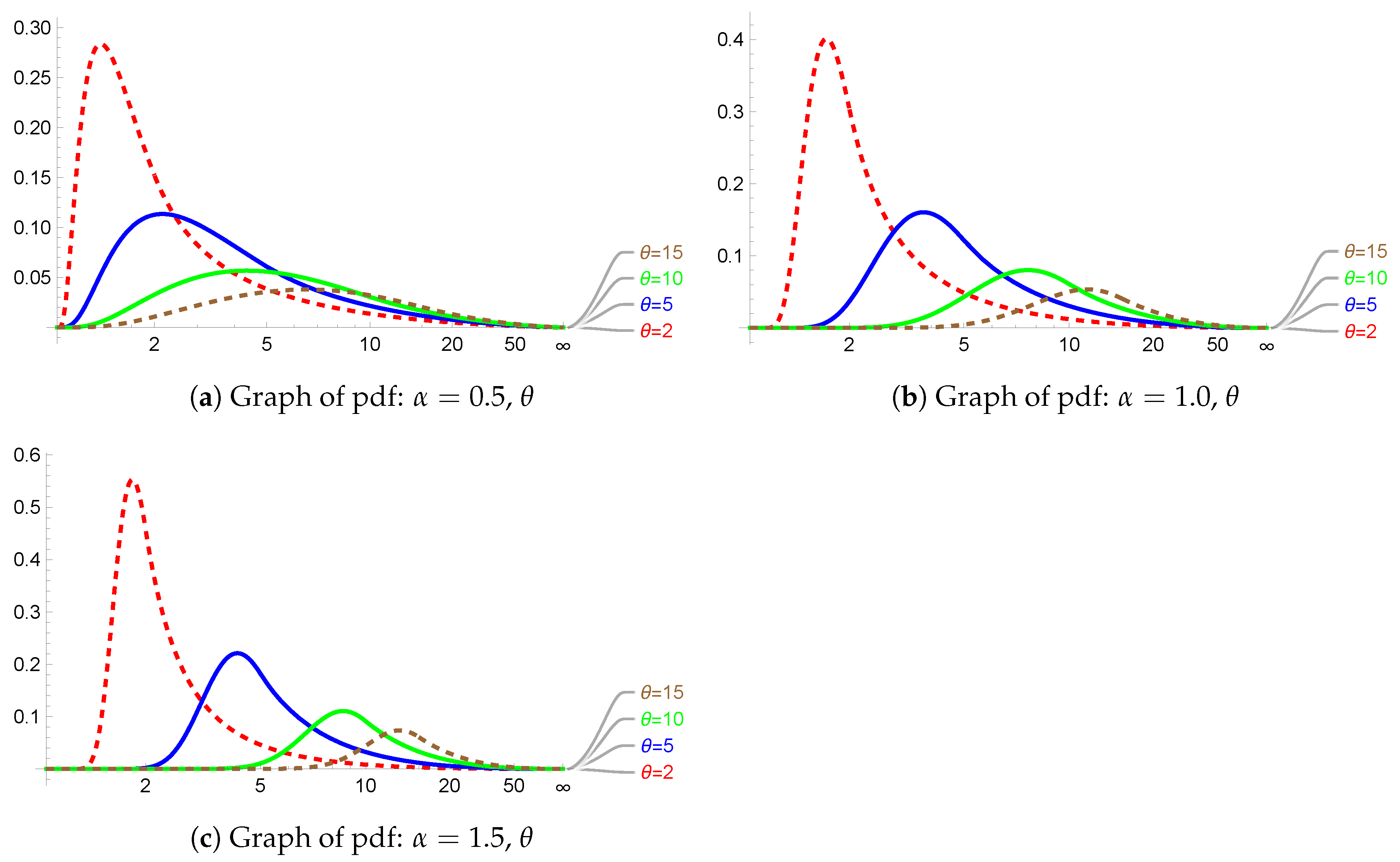
We observe that the original four parameters are reduced to two: $\alpha$ and $\theta$. Figure 1a–c show that for a fixed value of $\alpha$ the PDF is a smooth curve. For smaller values of $\alpha$ (corresponding to larger values of $\sigma$), the PDF is more heavily tailed.

• Value- at-Risk (VaR)

In actuarial science applications, an important risk measure is Value-at-Risk (VaR), which is used to assess risk exposure. VaR quantifies the potential loss an investment may incur at a given confidence level $1-\gamma$ and is defined as

$$Va{R}_{(1-\gamma )}=inf\left\{y|F_Y\left(y\right)\ge 1-\gamma \right\}.$$

The common values of $1-\gamma$ are 0.99 and 0.95. For composite distributions as a loss model, VaR lies in the second distribution $F_2\left(y\right)$. Based on the LogNormal–Pareto model,

$$Va{R}_{(1-\gamma )}=F_2^{-1}(1-\gamma )=\theta {\left({\displaystyle \frac{c}{\gamma }}\right)}^{\left({\displaystyle \frac{1}{\alpha }}\right)}.$$

For example, with $\theta =50$ and $\alpha =2.0$, and with $(1-\gamma )$ = $0.95$, we get $Va{R}_{\left(0.95\right)}=174.334$.

3. Maximum Likelihood Method for Parameters and Finding $\mathit{m}$

This section discusses computing the ML estimates of the parameters $\alpha$ and, consequently, $\theta$ for the PDF $f_Y\left(y\right)$ given in Section 2. Assume $y_1,y_2,\dots ,y_n\sim \mathrm{LogNormal}–\mathrm{Pareto}(\theta ,\alpha )$, with $y_1<y_2<\dots \le y_m<y_{m+1}<\dots <y_n$ for an integer m such that $1<m<n$. Assume that $y_1,y_2,\dots ,y_m$ and $y_{m+1},\dots ,y_n$ are, respectively, from the first and second components of the composite distribution. The likelihood function L is written as

$$L=c^n{\alpha }^n{\theta }^{n\alpha }{\displaystyle \prod _{i=1}^n}{y}_i^{-(\alpha +1)}{e}^{-{\sum }_{i=1}^m{\displaystyle \frac{{\alpha }^2}{2w^2}}{ln}^2(y_i/\theta )}$$

Following the algorithm in Deng et al. (2021), the MLEs are obtained as follows:

If $m=1$,

$$\widehat{\theta }=x_1{\left({\displaystyle \prod _{i=1}^m}{x}_i/x_1\right)}^{w^2},\widehat{\alpha }=m{\left({\displaystyle \sum _{i=1}^m}ln(x_i/x_1)\right)}^{-1}$$

otherwise,

$$\widehat{\theta }=e^{\left({\displaystyle \frac{n{w}^2}{m\widehat{\alpha }}}\right)}{\left({\displaystyle \prod _{i=1}^m}{x}_i\right)}^{{\displaystyle \frac{1}{m}}},\widehat{\alpha }={\displaystyle \frac{w^{2}B+\sqrt{w^4{B}^2+4mn{w}^{2}A}}{2A}},$$

where $A=m{\sum }_{i=1}^m{\left(ln\left(x_i\right)\right)}^2-{\left({\sum }_{i=1}^{m}ln\left(x_i\right)\right)}^2$, $B=n{\sum }_{i=1}^{m}ln\left(x_i\right)-m{\sum }_{i=1}^{n}ln\left(x_i\right)$.

In the simulation studies, a code similar to Code A (see Supplementary Materials) uses selected “true” values ${\alpha }_t$ and ${\theta }_t$ to generate $N=100$ samples of size n from the composite distribution. For each generated sample, the correct value of m is determined and then used to compute the MLEs. The mean of the MLE and the average squared error (ASE), denoted by $\xi$, are listed in

Table 1. Accuracy of ML estimator for $\theta$ and $\alpha$.

n	${\mathit{\alpha }}_{\mathit{t}}$	$\overline{\widehat{\mathit{\alpha }}}$	$\mathit{\xi }\left(\widehat{\mathit{\alpha }}\right)$	${\mathit{\theta }}_{\mathit{t}}$	$\overline{\widehat{\mathit{\theta }}}$	$\mathit{\xi }\left(\widehat{\mathit{\theta }}\right)$
100	0.5	0.5047	(0.0019)	2	2.0297	(0.0835)
150	0.5	0.5014	(0.0010)	2	2.0091	(0.0457)
100	0.5	0.5110	(0.0022)	10	10.1583	(1.6353)
150	0.5	0.5019	(0.0016)	10	10.0368	(1.1477)
100	0.5	0.5111	(0.0023)	15	15.2412	(4.7998)
150	0.5	0.5058	(0.0018)	15	15.4338	(2.7620)
100	1.5	1.5145	(0.0209)	2	2.0025	(0.0085)
150	1.5	1.5105	(0.0130)	2	1.9992	(0.0064)
100	1.5	1.5355	(0.0232)	10	10.042	(0.2242)
150	1.5	1.5271	(0.0145)	10	9.9592	(0.1022)
100	1.5	1.5187	(0.0193)	15	14.9662	(0.4716)
150	1.5	1.4880	(0.0144)	15	15.0986	(0.3921)

.

Table 1 reveals that as the sample size n increases, the ASE for the estimators, defined as

$$\xi \left(\widehat{\alpha }\right)={\displaystyle \frac{{\sum }_{j=1}^N{({\widehat{\alpha }}_j-{\alpha }_t)}^2}{N}}\xi \left(\widehat{\theta }\right)={\displaystyle \frac{{\sum }_{j=1}^N{({\widehat{\theta }}_j-{\theta }_t)}^2}{N}},$$

decreases for all values of ${\alpha }_t$ and ${\theta }_t$ listed in Table 1. Also, for specific combinations of $({\alpha }_t,{\theta }_t)$ with the same ${\theta }_t$, a larger ${\alpha }_t$ yields a smaller $\xi \left(\widehat{\theta }\right)$. Similarly, when ${\alpha }_t$ is held fixed a smaller ${\theta }_t$ yields a smaller $\xi \left(\widehat{\alpha }\right).$ A visual summary of the results in Table 1 is shown in Figure 2.

4. Regression Model

Suppose there are p potential covariates, $x_1,\dots ,x_p$ associated with the loss variable Y. For each row $x_i^{\prime }=(x_{i1},\dots ,x_{ip})$, $i=1,2,\dots ,k$ in the design matrix $X_{(k\times p)}$ let $y_i$ be a realization of the response variable Y from the LogNormal–Pareto composite PDF. Without loss of generality, assume the ordered sample $y_1<y_2<\dots <y_m<y_{m+1},\dots <y_k$, where $y_1,\dots ,y_m$ come from the LogNormal and $y_{m+1},\dots ,y_k$ from the Pareto.

Let us rewrite PDF (4) utilizing $\alpha ={\displaystyle \frac{w}{\sigma }}$; we get

$$f_Y\left(y\right)=\left\{\begin{array}{cc}c\left({\displaystyle \frac{w}{\sigma }}\right){\theta }^{\left({\displaystyle \frac{w}{\sigma }}\right)}{y}^{-({\displaystyle \frac{w}{\sigma }}+1)}{e}^{-{\displaystyle \frac{{ln}^2(y/\theta )}{2{\sigma }^2}}}\hfill & 0<y\le \theta \hfill \\ c\left({\displaystyle \frac{w}{\sigma }}\right){\theta }^{\left({\displaystyle \frac{w}{\sigma }}\right)}{y}^{-({\displaystyle \frac{w}{\sigma }}+1)}\hfill & \theta \le y<\infty \hfill \end{array}\right.$$

The advantage of the above parameterization is that it directly involves the scale parameter $\sigma$ of the LogNormal distribution, with larger $\sigma$ yielding a more heavily tailed PDF. The regression parameters are denoted by ${\beta }^{\prime }=({\beta }_1,{\beta }_2,\dots ,{\beta }_p)$. To define a link function in regression modeling, the threshold parameter ${\theta }_i$ must be associated with the p covariates. The constraint is that ${\theta }_i$, for given covariate values $x_{i1},\dots ,x_{ip},i=1,2,\dots ,k$, must be positive. Choices like ${\theta }_i=x_i^{\prime }\beta$ or ${\theta }_i=ln\left(x_i^{\prime }\beta \right)$ are not mathematically feasible because, due to dependence on the covariate data, ${\theta }_i$ may not be positive. In that article, we chose ${\theta }_i=e^{x_i^{\prime }\beta },i=1,2,\dots ,k$, as the link function. If covariate values are large, rescaling them is recommended to avoid overflow when applying the link function.

With the link function and covariates, the loglikelihood function l for the LogNormal–Pareto composite distribution can be expressed as

$$l\propto -kln\left(\sigma \right)-\left({\displaystyle \frac{w}{\sigma }}\right){\displaystyle \sum _{i=1}^k}{x}_i^{\prime }\beta -(1+{\displaystyle \frac{w}{\sigma }}){\displaystyle \sum _{i=1}^k}ln\left(y_i\right)-0.5{\sigma }^{-2}{\displaystyle \sum _{i=1}^m}{(ln\left(y_i\right)-x_i^{\prime }\beta )}^2.$$

There are $p+1$ parameters, including $\sigma$, that should be estimated by optimizing the likelihood function.

ML Estimation for Regression Parameters

This section presents the computation of MLEs of the regression parameters. The variance–covariance matrix of the estimators is obtained from the Fisher information matrix, which is then used to identify insignificant covariates. Using matrix notation, the log-likelihood function, based on a random sample $\underline{y}$ on Y, and a $k\times p$ design matrix X,

$$\underline{y}=\left[\begin{array}{c}{y}_1\\ y_2\\ ⋮\\ y_m\\ y_{m+1}\\ ⋮\\ y_k\end{array}\right]X_{k\times p}=\left[\begin{array}{c}{x}_1^{\prime }\\ x_2^{\prime }\\ ⋮\\ x_m^{\prime }\\ x_{m+1}^{\prime }\\ ⋮\\ x_k^{\prime }\end{array}\right]$$

can be expressed as,

$$l\propto -kln\left(\sigma \right)+\left({\displaystyle \frac{w}{\sigma }}\right)1^{\prime }X\beta -(1+{\displaystyle \frac{w}{\sigma }})1^{\prime }ln\left(y^{*}\right)-0.5{\sigma }^{-2}{\left(ln\left(y^{*}\right)-X^{*}\beta \right)}^{\prime }\left(ln\left(y^{*}\right)-X^{*}\beta \right),$$

where

$${\underline{y}}^{*}=\left[\begin{array}{c}{y}_1\\ y_2\\ ⋮\\ y_m\end{array}\right]X_{m\times p}^{*}=\left[\begin{array}{c}{x}_1^{\prime }\\ x_2^{\prime }\\ ⋮\\ x_m^{\prime }\end{array}\right]1_{k\times 1}=\left[\begin{array}{c}1\\ 1\\ ⋮\\ 1\end{array}\right]1_{m\times 1}^{*}=\left[\begin{array}{c}1\\ 1\\ ⋮\\ 1\end{array}\right].$$

Differentiating l with respect to $\sigma$ and ${\beta }_1,\dots ,{\beta }_p$ yields the following equations:

$${\displaystyle \frac{\partial l}{\partial \sigma }}=k{\sigma }^2+\sigma w{1}^{\prime }X\beta -\sigma w{1}^{\prime }ln\left(\underline{y}\right)-l{n}^{\prime }\left({\underline{y}}^{*}\right)ln\left({\underline{y}}^{*}\right)+2{ln}^{\prime }\left({\underline{y}}^{*}\right)X^{*}\beta -{\beta }^{\prime }{X}^{{*}^{\prime }}{X}^{*}\beta =0,$$

(5)

$${\displaystyle \frac{\partial l}{\partial {\beta }_g}}=w\sigma 1^{\prime }{x}_g-l{n}^{\prime }\left({\underline{y}}^{*}\right)x_g^{*}+{\beta }_g{x}_g^{{*}^{\prime }}{x}_g^{*}-{\displaystyle \sum _{h\ne g}^m}{\beta }_h{x}_g^{{*}^{\prime }}{x}_h^{*}=0,g,h=1,2,\dots ,p.$$

(6)

Equations (5) and (6) can be solved simultaneously for the $p+1$ parameters to obtain exact solutions; there is no need to use an optimization program, such as Mathematica’s NMaximize, to maximize the likelihood function. In the following, we present explicit formulas for the MLEs of the regression parameters for the $p=2$ and $p=3$ cases.

• The p = 2 Case

From (5) and (6), we get

$${\beta }_1={\displaystyle \frac{{\beta }_2(A_1{A}_2-A2A_5)+A_2{A}_6-A_1{A}_7}{A_2{A}_3-A_1{A}_5}},\sigma ={\displaystyle \frac{-S_1+\sqrt{S_1^2+4k{S}_2}}{2k}},$$

(7)

where

$$S_1=w{\displaystyle \sum _{i=1}^k}{\beta }_1{x}_{i,1}+{\beta }_2{x}_{i,2}-ln\left(y_i\right),S_2={\displaystyle \sum _{i=1}^k}{\left(ln\left(y_i\right)-{\beta }_1{x}_{i,1}-{\beta }_2{x}_{i,2}\right)}^2,$$

$$A_1={\displaystyle \sum _{i=1}^k}{x}_{i,1},A_2={\displaystyle \sum _{i=1}^k}{x}_{i,2},A_3={\displaystyle \sum _{i=1}^m}{x}_{i,1}^2,A_4={\displaystyle \sum _{i=1}^m}{x}_{i,2}^2,$$

$$A_5={\displaystyle \sum _{i=1}^m}{x}_{i,1}{x}_{i,2},A_6={\displaystyle \sum _{i=1}^m}{x}_{i,1}ln\left(y_i\right),A_7={\displaystyle \sum _{i=1}^m}{x}_{i,2}ln\left(y_i\right),$$

Note that $\sigma$, throughout $S_1$ and $S_2$, depends on ${\beta }_2$. Therefore, using (7), ${\widehat{\beta }}_2$ is the unique solution to the equation

$${\displaystyle \frac{\partial l}{\partial {\beta }_1}}=w\sigma A_1+A6-{\beta }_1{A}_3+{\beta }_2{A}_5=0.$$

Consequently, ${\widehat{\beta }}_1$ and $\widehat{\sigma }$ can be computed using (7). Code B (see Supplementary Materials) computes the MLEs of the regression parameters for the p = 2 case.

• The p = 3 Case

From (6), we get three equations:

$${\displaystyle \frac{-B_{10}+{\beta }_1{B}_4+{\beta }_3{B}_7+{\beta }_2{B}_8}{B_1}}={\displaystyle \frac{-B_{11}+{\beta }_2{B}_5+{\beta }_1{B}_8+{\beta }_3{B}_9}{B_2}}$$

$${\displaystyle \frac{-B_{10}+{\beta }_1{B}_4+{\beta }_3{B}_7+{\beta }_2{B}_8}{B_1}}={\displaystyle \frac{-B_{12}+{\beta }_3{B}_6+{\beta }_2{B}_9+{\beta }_1{B}_7}{B_3}}$$

$${\displaystyle \frac{-B_{11}+{\beta }_2{B}_5+{\beta }_1{B}_8+{\beta }_3{B}_9}{B_2}}={\displaystyle \frac{-B_{12}+{\beta }_3{B}_6+{\beta }_2{B}_9+{\beta }_1{B}_7}{B_3}},$$

(8)

where

$$B_1={\displaystyle \sum _{i=1}^k}{x}_{i,1},B_2={\displaystyle \sum _{i=1}^k}{x}_{i,2},B_3={\displaystyle \sum _{i=1}^k}{x}_{i,3},B_4={\displaystyle \sum _{i=1}^m}{x}_{i,1}^2,B_5={\displaystyle \sum _{i=1}^m}{x}_{i,2}^2,B_6={\displaystyle \sum _{i=1}^m}{x}_{i,3}^2$$

$$B_7={\displaystyle \sum _{i=1}^m}{x}_{i,1}{x}_{i,3},B_8={\displaystyle \sum _{i=1}^m}{x}_{i,1}{x}_{i,2},B_9={\displaystyle \sum _{i=1}^m}{x}_{i,2}{x}_{i,3},B_{10}={\displaystyle \sum _{i=1}^m}{x}_{i,1}ln\left(y_i\right),$$

$$B_{11}={\displaystyle \sum _{i=1}^m}{x}_{i,2}ln\left(y_i\right),B_{12}={\displaystyle \sum _{i=1}^m}{x}_{i,3}ln\left(y_i\right),B_{13}={\displaystyle \sum _{i=1}^m}ln\left(y_i\right),B_{14}={\displaystyle \sum _{i=1}^m}{ln}^2\left(y_i\right).$$

Utilizing Equation (8) simultaneously, ${\beta }_2$ and ${\beta }_3$ are expressed in terms of ${\beta }_1$. From (5), we get

$$w\sigma B_1=-B_{10}+{\beta }_1{B}_4+{\beta }_3{B}_7+{\beta }_2{B}_8,$$

(9)

which expresses $\sigma$ in terms of ${\beta }_1$. Consequently, the positive solution to (10) is $\widehat{\sigma }$. Then, the MLEs of ${\beta }_g$, $g=1,2,3$ are computed:

$$k{\sigma }^2+w\sigma ({\beta }_1{B}_1+{\beta }_2{B}_2+{\beta }_3{B}_3-B_{13})-B_{14}+2y^{{*}^{\prime }}{X}^{*}\beta -{\left(X^{*}\beta \right)}^{\prime }\left(X^{*}\beta \right)=0.$$

(10)

Code C (see the Supplementary Materials) computes the MLEs of the regression parameters for the p = 3 case.

Some predictors may be insignificant. We propose using the Fisher information matrix and Wald’s test to identify them. Using the log-likelihood function l in Section “ML Estimation for Regression Parameters”, let

$$I_{\beta }={\displaystyle \frac{\partial l}{\partial \beta }}{I}_{\beta \beta }={\displaystyle \frac{\partial I_{\beta }}{\partial \beta }}.$$

(11)

$I_{\beta }$ is a $p\times 1$ vector. The objective is to compute IFM = ${\left(E\left[I_{\beta \beta }\right]\right)}^{-1}{|}_{\beta =\widehat{\beta }}$, which is the inverse of the estimated Fisher information matrix. IFM is the variance–covariance matrix of $\widehat{\beta }$. In this article, the Fisher scoring algorithm for the parameter estimates,

$${\widehat{\beta }}_{v+1}={\widehat{\beta }}_v-{\left(E\left[I_{\beta \beta }\right]\right)}^{-1}·I_{\beta }{|}_{\beta ={\widehat{\beta }}_v}$$

(12)

where v is the iteration index, is not employed because closed-form formulas are presented for the $p=2$ and $p=3$ cases, and for the general case $p>3$ a numerical optimization in Mathematica can be used to maximize the log-likelihood and determine the MLEs. Computation of the Fisher information matrix is necessary to identify statistically significant predictors in the regression model.

It can be verified, based on the likelihood function, l, that $I_{\beta \beta }$ does not involve $Y_1,\dots ,Y_m,Y_{m+1},\dots ,Y_n$; consequently, the computation of IFM does require estimating the expected values,

$$E\left[Y_i\right|Y_i<{\theta }_i]=0.303925e^{{\displaystyle \frac{{\sigma }^2(0.0692809-\frac{0.138562w)}{\sigma }}{w^2}}}{\theta }_i(1+Erf(0.263213-{\displaystyle \frac{0.263213\sigma }{w}}),$$

$$E\left[Y_i\right|Y_i>{\theta }_i]={\displaystyle \frac{cw{\theta }_i}{(w-\sigma )}},$$

(13)

by replacing the parameters in (13) with their MLEs.

We propose using Wald’s test statistic

$$W_g={\displaystyle \frac{{\widehat{\beta }}_g}{\sqrt{IF{M}_{\left(gg\right)}}}},g=1,2,\dots ,p,$$

where the diagonal element of ${\mathrm{IFM}}_{\left(gg\right)}$ estimates the variance of $\widehat{{\beta }_g}$. Due to the asymptotic properties of MLEs, ${\widehat{\beta }}_1,\dots ,{\widehat{\beta }}_p$ are asymptotically normally distributed when the sample size k is large. $|W_g|$ can be compared with a critical value from the standard normal distribution to identify insignificant predictors. This process continues until all remaining predictors in the model are significant.

5. Bayesian Estimation of Regression Parameters

Selecting a conjugate prior distribution can be challenging, especially when the goal is for the posterior to belong to the same class as the prior. Additionally, the posterior PDF may not be in a recognizable form, complicating the derivation of the Bayes estimator as the posterior’s expected value. In these situations, a computational approach is to use a Markov Chain Monte Carlo (MCMC) algorithm. It requires selecting a proposal distribution for the posterior, which may not belong to any well-known class of distributions. The algorithm then runs simulations until convergence is confirmed. Aminzadeh and Deng (2022) used an MCMC algorithm to obtain a Bayes estimate of the renewal function when the interarrival times follows a Pareto distribution.

Since the regression parameters ${\beta }_1,{\beta }_2,\dots ,{\beta }_p$ can take any value, and their MLEs based on a large sample are approximately normally distributed, we propose the multivariate normal distribution as a prior. Let

$$\underline{\beta }\sim N_p(\varphi ,\Sigma ),\underline{\beta }=({\beta }_1,\dots ,{\beta }_p),$$

(14)

where $E\left({\beta }_j\right)={\varphi }_j,j=1,2,\dots ,p$. The matrix $\Sigma$ is the $p\times p$ positive-definite variance–covariance matrix of ${\beta }_1,\dots ,{\beta }_p.$

Using the likelihood function and (14), the posterior can be written as

$${\displaystyle \prod _{i=1}^k}{\displaystyle \frac{cw}{\sigma }}{y}_i^{-(1+{\displaystyle \frac{w}{\sigma )}}}{\displaystyle \prod _{i=1}^m}{e}^{-{\displaystyle \frac{1}{2{\sigma }^2}}{\left(ln\left(y_i\right)-x_i^{\prime }\beta \right)}^2}$$

$$\times {\left(2\pi \right)}^{p/2}{[det(\Sigma )]}^{-0.5}{e}^{-0.5{(\underline{\beta }-\underline{\varphi })}^{\prime }{\Sigma }^{-1}(\underline{\beta }-\underline{\varphi })}.$$

(15)

The number of hyperparameters is $p+\left({\displaystyle \genfrac{}{}{0pt}{}{p}{2}}\right)$ in the prior distribution. They are ${\varphi }_j$ ($j=1,2,\dots ,p$) as well as the covariances $\mathrm{Cov}({\beta }_i,{\beta }_j)$ (for $i\ne j$ and $i,j=1,2,\dots ,p$). Data-driven approaches based on MLEs are used in the literature to assign hyperparameter values, as in Aminzadeh and Deng (2025) and Aminzadeh and Deng (2022), when relevant information about the parameters is unavailable. This involves using MLEs to compute the hyperparameter governing the prior mean while simultaneously minimizing the prior variance. The simulation studies reported in the articles confirm that this method yields more accurate Bayesian estimates than MLEs.

5.1. Approximate Bayesian Computation

The ABC algorithm dates back to the 1980s, when Donald Rubin introduced it. Lintusaari et al. (2017) provided a comprehensive overview of recent developments in the ABC method. Researchers have employed this method, mainly when the posterior probability density function (PDF) is intractable. We turned to the ABC algorithm, which relies on extensive simulations, because the posterior in (15) is challenging to work with. It is worth noting that the proposed ABC method presented in this article is preferred over alternative Bayesian methods, such as classical Bayesian methods, because with many covariates in the regression model selecting hyperparameter values for the regression parameters is extremely difficult, if not impossible. Alternative Bayesian computational methods, such as MCMC, are not useful because the posterior distribution (15) is intractable. In addition, the multivariate normal distribution is an appropriate prior given the asymptotic properties of MLEs.

5.2. Computation Steps for ML and ABC Estimates Using Simulated Data

For selected “true” values of ${\sigma }_t$ and ${\beta }_t=({\beta }_{t,1},\dots ,{\beta }_{t,p})$ and a chosen $k\times p$ design matrix X, we generate $N_S=300$ samples $y_{j1},\dots ,y_{jk}$ for $j=1,2,\dots ,N_S$ from the LogNormal–Pareto composite distribution. The following steps in Mathematica Code A compute the MLEs and approximate Bayesian estimates of ${\beta }_{t1},\dots ,{\beta }_{tp}$:

1.

In the $jth$ iteration $j=1,2,\dots ,N_S$, software such as Mathematica (as shown for $p=2$ and $p=3$ cases in Section 4) is used to solve

$${\displaystyle \frac{\partial l}{\partial \sigma }}=k{\sigma }^2+\sigma w{1}^{\prime }X\beta -\sigma w{1}^{{*}^{\prime }}ln\left({\underline{y}}^{*}\right)-l{n}^{\prime }\left({\underline{y}}^{*}\right)ln\left({\underline{y}}^{*}\right)+{ln}^{\prime }\left({\underline{y}}^{*}\right)X^{*}\beta +{\beta }^{\prime }{X}^{{*}^{\prime }}ln\left({\underline{y}}^{*}\right)-{\beta }^{\prime }{X}^{{*}^{\prime }}{X}^{*}\beta =0,$$

$${\displaystyle \frac{\partial l}{\partial {\beta }_g}}=w\sigma 1^{\prime }{x}_g-l{n}^{\prime }\left({\underline{y}}^{*}\right)x_g^{*}+{\beta }_g{x}_g^{{*}^{\prime }}{x}_g^{*}-{\displaystyle \sum _{h\ne g}^m}{\beta }_h{x}_g^{{*}^{\prime }}{x}_h^{*}=0,g,h=1,2,\dots ,p$$

simultaneously to find the MLEs: $\widehat{\sigma },{\widehat{\beta }}_1,\dots ,{\widehat{\beta }}_p$ and to use Wald’s test statistic to identify significant predictors to retain in the model. Assuming that all predictors are retained in the model, the MLEs based on $NS$ samples are computed as

$${\widehat{\sigma }}_{\mathrm{ML}}={\displaystyle \frac{{\sum }_{j=1}^{N_S}{\widehat{\sigma }}_j}{N_S}},{\widehat{\beta }}_{\mathrm{ML},\mathrm{g}}={\displaystyle \frac{{\sum }_{j=1}^{N_S}{\widehat{\beta }}_{jg}}{N_S}},{\widehat{\beta }}_{ML}=({\widehat{\beta }}_{\mathrm{ML},1},\dots ,{\widehat{\beta }}_{\mathrm{ML},\mathrm{p}})$$

and with ASEs,

$$\xi \left({\widehat{\sigma }}_{\mathrm{ML}}\right)={\displaystyle \frac{{\sum }_{j=1}^{N_S}{({\widehat{\sigma }}_j-{\sigma }_t)}^2}{N_S}},\xi \left({\widehat{\beta }}_{\mathrm{ML},\mathrm{g}}\right)={\displaystyle \frac{{\sum }_{j=1}^{N_S}{({\widehat{\beta }}_{\mathrm{ML},\mathrm{g}}-{\beta }_{t,g})}^2}{N_S}},g=1,2,\dots ,p.$$

For the jth generated sample, $j=1,2,\dots ,N_S$, ${\mathrm{IFM}}_j$ matrix is computed, and then the overall variance–covariance matrix

$$\mathrm{IFM}={\displaystyle \frac{{\sum }_{j=1}^{N_S}{\mathrm{IFM}}_j}{N_S}}$$

is obtained.

2.

Generate $Nss=3000$ random samples from a multivariate Normal distribution $N_p({\widehat{\beta }}_{ML},\mathrm{IFM})$. ${\beta }_1^v,\dots ,{\beta }_p^v$ is the vth generated sample, $v=1,2,\dots ,Nss$.

3.

Use ${\beta }^v=({\beta }_1^v,\dots ,{\beta }_p^v)$ to generate a sample of size k from the composite distribution with the ith row $x_i^{\prime }$ of the matrix X and the link function ${\theta }_i=e^{x_i^{\prime }{\beta }^v}$. The simulated samples are denoted by $y_1^v,y_2^v,\dots ,y_k^v,v=1,2,\dots ,Nss$.

4.

Compare the simulated samples $y_1^v,y_2^v,\dots ,y_k^v$ with $y_{j1},..,y_{jk}j=1,2,\dots ,N_S$ using selected summary statistics. Per the ABC method, it is desired to have “small” differences in the selected summary statistics. Add the $v^{th}$ simulated ${\beta }^v$ from Step 3 to the set of “accepted samples” from the posterior distribution if the difference in the selected summary statistics is less than the tolerance $ϵ$. We use the 30th and 90th percentiles as summary statistics. This choice reflects the characteristics of loss data in the insurance industry, which include frequent small losses and infrequent large losses. Therefore, percentiles such as the 30th and 90th are used to assess agreement between the original and simulated data. If we compare summary statistics such as means or sums, a few extreme values at the high end of the simulated and original samples can heavily distort the metric, whereas percentiles isolate values by their relative position. Therefore, for a more accurate comparison, percentiles are employed; ${ϵ}_1$ and ${ϵ}_2$ respectively denote the tolerance errors for the 30th and 90th percentiles. There are $N_S$ original samples from Step 1 and $Nss$ samples in Step 3. In the simulation studies, all $N_{ss}$ samples were compared with a random sample drawn from the $N_S$ samples. This choice reflected the practical case, as in an actual application only one sample is available for analysis.

5.

Let $N_a$ denote the number of acceptable simulated samples ${\beta }_1^{\nu },\dots ,{\beta }_p^{\nu }$. Define an ABC-based estimate as

$${\widehat{\beta }}_{\mathrm{Bayes},g}={\displaystyle \frac{{\sum }_{h=1}^{N_a}{\beta }_g^h}{N_a}},$$

with the ASE,

$$\xi ({\widehat{\beta }}_{\mathrm{Bayes},\mathrm{g})}={\displaystyle \frac{{\sum }_{h=1}^{N_a}{({\widehat{\beta }}_{\mathrm{Bayes},g}-{\beta }_{t,g})}^2}{N_a}},g=1,2,\dots ,p.$$

(16)

The choice of the tolerance parameters ${ϵ}_1$ and ${ϵ}_2$ depends mainly on the $y_1,y_2,\dots ,y_k$ and the simulated sample. Small tolerance values would lead to a small $N_a$, which is undesirable, and large tolerance values would force $N_a$ to be close to $N_{ss}$, which is also undesirable, as MLE and ABC estimates would be almost identical. Before making all the comparisons in Step 4, it is recommended to print a few absolute differences between the percentiles to inform the appropriate choices of ${ϵ}_1$ and ${ϵ}_2$. As we implement the ABC method in the code and check the acceptance status of each simulated sample, if the majority (e.g., 80%) of the first few samples are accepted or only a very few (e.g., 5%) are accepted, then the tolerance parameter values must be adjusted.

6. Simulation: Regression Model

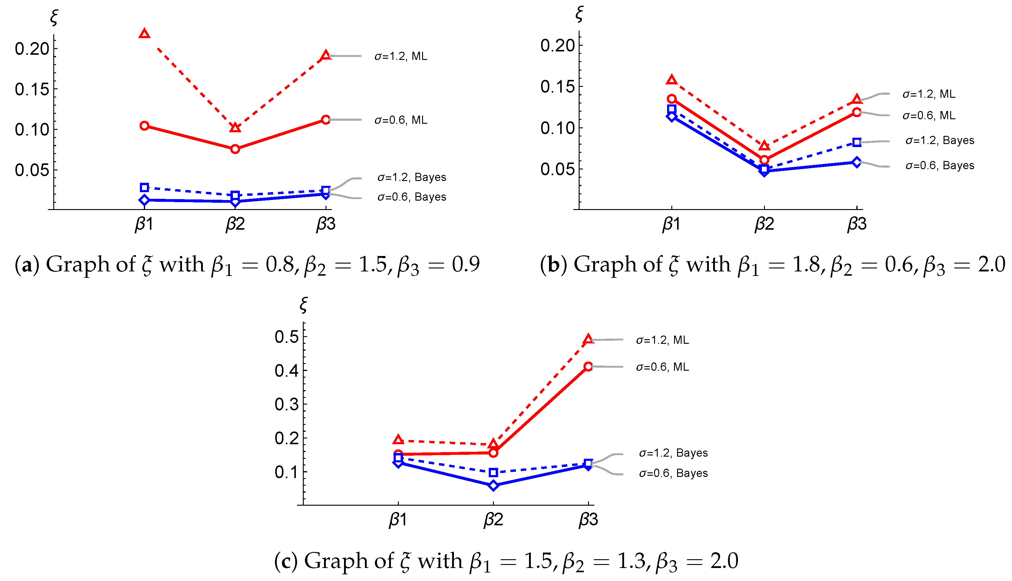
This section presents our simulation results from the LogNormal–Pareto model using a variety of selected values for the number of covariates (p), “true” values for the regression parameters ${\beta }_1,\dots ,{\beta }_p$, and “true” values for $\sigma$. The objective of these simulations was to demonstrate that the proposed ABC method outperforms ML in estimator accuracy, as measured by ASE.

Using sample sizes $k=50,k=100,k=300$ and ${\beta }_t$, ${\sigma }_t$, and p, we generated $N_S=300$ samples from the composite distribution to obtain the MLEs. We then generated $Nss=3000$ samples from a multivariate normal distribution and implemented the ABC algorithm to obtain Bayesian estimates of the regression parameters.

In our simulation studies, for convenience, a $k\times p$ design matrix X was generated from a Uniform distribution. Notably, the same matrix X was used across all $N_S$ simulations, based on input parameters $k,{\sigma }_t,$ and ${\beta }_t$. The choice of distribution for X and the parameter values for the Uniform distribution were irrelevant and did not affect the main results reported in the article regarding the accuracies of the ML and ABC estimates.

Table 2. Comparison of ML and ABC accuracies for k = 50.

					${\beta }_1=0.2$	${\beta }_2=0.5$
				ML				Bayes
${\sigma }_t$	${\overline{\widehat{\sigma }}}_{ML}$	${\xi }_{{\widehat{\sigma }}_{MLE}}$	${\overline{\widehat{{\beta }_1}}}_{MLE}$	${\xi }_{{\beta }_{1MLE}}$	${\overline{\widehat{{\beta }_2}}}_{MLE}$	${\xi }_{{\beta }_{2MLE}}$	${\overline{\widehat{{\beta }_1}}}_{Bayes}$	${\xi }_{{\beta }_{1Bayes}}$	${\overline{\widehat{{\beta }_2}}}_{Bayes}$	${\xi }_{{\beta }_{2Bayes}}$
0.6	0.5979	(0.0045)	0.2185	(0.0531)	0.5283	(0.0543)	0.2247	(0.0375)	0.5174	(0.0451)
1.2	1.1814	(0.0235)	02224	(0.1745)	0.5164	(0.1172)	0.2344	(0.0540)	0.4679	(0.0675)
					${\beta }_1=1.2$	${\beta }_2=0.5$
${\sigma }_t$	${\overline{\widehat{\sigma }}}_{ML}$	${\xi }_{{\widehat{\sigma }}_{MLE}}$	${\overline{\widehat{{\beta }_1}}}_{MLE}$	${\xi }_{{\beta }_{1MLE}}$	${\overline{\widehat{{\beta }_2}}}_{MLE}$	${\xi }_{{\beta }_{2MLE}}$	${\overline{\widehat{{\beta }_1}}}_{Bayes}$	${\xi }_{{\beta }_{1Bayes}}$	${\overline{\widehat{{\beta }_2}}}_{Bayes}$	${\xi }_{{\beta }_{2Bayes}}$
0.6	0.7064	(0.0198)	1.6020	(0.1025)	0.4174	(0.0384)	1.5726	(0.0252)	0.4666	(0.0241)
1.2	1.2431	(0.0320)	1.3773	(0.1858)	0.5034	(0.0494)	1.3738	(0.0806)	0.5198	(0.0347)
					${\beta }_1=0.6$	${\beta }_2=1.5$
${\sigma }_t$	${\overline{\widehat{\sigma }}}_{ML}$	${\xi }_{{\widehat{\sigma }}_{MLE}}$	${\overline{\widehat{{\beta }_1}}}_{MLE}$	${\xi }_{{\beta }_{1MLE}}$	${\overline{\widehat{{\beta }_2}}}_{MLE}$	${\xi }_{{\beta }_{2MLE}}$	${\overline{\widehat{{\beta }_1}}}_{Bayes}$	${\xi }_{{\beta }_{1Bayes}}$	${\overline{\widehat{{\beta }_2}}}_{Bayes}$	${\xi }_{{\beta }_{2Bayes}}$
0.6	0.6832	(0.0198)	0.6402	(0.0484)	1.6648	(0.0689)	0.6494	(0.0255)	1.6615	(0.0370)
1.2	1.2551	(0.0313)	0.6465	(0.2012)	1.6385	(0.1358)	0.6204	(0.0604)	1.6433	(0.0492)
					${\beta }_1=1.2$	${\beta }_2=1.5$
${\sigma }_t$	${\overline{\widehat{\sigma }}}_{ML}$	${\xi }_{{\widehat{\sigma }}_{MLE}}$	${\overline{\widehat{{\beta }_1}}}_{MLE}$	${\xi }_{{\beta }_{1MLE}}$	${\overline{\widehat{{\beta }_2}}}_{MLE}$	${\xi }_{{\beta }_{2MLE}}$	${\overline{\widehat{{\beta }_1}}}_{Bayes}$	${\xi }_{{\beta }_{1Bayes}}$	${\overline{\widehat{{\beta }_2}}}_{Bayes}$	${\xi }_{{\beta }_{2Bayes}}$
0.6	0.6699	(0.0123)	1.2905	(0.0792)	1.6831	(0.1068)	1.2276	(0.0329)	1.6993	(0.0477)
1.2	1.2564	(0.0234)	1.4067	(0.1471)	1.5512	(0.1126)	1.3774	(0.0603)	1.5700	(0.0837)

,

Table 3. Comparison of ML and ABC accuracies for k = 100.

					${\beta }_1=0.2$	${\beta }_2=0.5$
				ML				Bayes
${\sigma }_t$	${\overline{\widehat{\sigma }}}_{ML}$	${\xi }_{{\widehat{\sigma }}_{MLE}}$	${\overline{\widehat{{\beta }_1}}}_{MLE}$	${\xi }_{{\beta }_{1MLE}}$	${\overline{\widehat{{\beta }_2}}}_{MLE}$	${\xi }_{{\beta }_{2MLE}}$	${\overline{\widehat{{\beta }_1}}}_{Bayes}$	${\xi }_{{\beta }_{1Bayes}}$	${\overline{\widehat{{\beta }_2}}}_{Bayes}$	${\xi }_{{\beta }_{2Bayes}}$
0.6	0.6260	(0.0042)	0.2023	(0.0201)	0.5467	(0.0161)	0.2185	(0.0144)	0.5323	(0.0067)
1.2	1.1814	(0.0126)	0.1842	(0.0395)	0.5085	(0.0277)	0.2175	(0.0153)	0.5209	(0.0093)
					${\beta }_1=1.2$	${\beta }_2=0.5$
${\sigma }_t$	${\overline{\widehat{\sigma }}}_{ML}$	${\xi }_{{\widehat{\sigma }}_{MLE}}$	${\overline{\widehat{{\beta }_1}}}_{MLE}$	${\xi }_{{\beta }_{1MLE}}$	${\overline{\widehat{{\beta }_2}}}_{MLE}$	${\xi }_{{\beta }_{2MLE}}$	${\overline{\widehat{{\beta }_1}}}_{Bayes}$	${\xi }_{{\beta }_{1Bayes}}$	${\overline{\widehat{{\beta }_2}}}_{Bayes}$	${\xi }_{{\beta }_{2Bayes}}$
0.6	0.6791	(0.0101)	1.5607	(0.2019)	0.4313	(0.0212)	1.2548	(0.0107)	0.4349	(0.0093)
1.2	1.2397	(0.0126)	1.3955	(0.2239)	0.4734	(0.0404)	1.2828	(0.0328)	0.4602	(0.0205)
					${\beta }_1=0.6$	${\beta }_2=1.5$
${\sigma }_t$	${\overline{\widehat{\sigma }}}_{ML}$	${\xi }_{{\widehat{\sigma }}_{MLE}}$	${\overline{\widehat{{\beta }_1}}}_{MLE}$	${\xi }_{{\beta }_{1MLE}}$	${\overline{\widehat{{\beta }_2}}}_{MLE}$	${\xi }_{{\beta }_{2MLE}}$	${\overline{\widehat{{\beta }_1}}}_{Bayes}$	${\xi }_{{\beta }_{1Bayes}}$	${\overline{\widehat{{\beta }_2}}}_{Bayes}$	${\xi }_{{\beta }_{2Bayes}}$
0.6	0.6621	(0.0069)	0.5855	(0.0164)	1.6616	(0.0448)	0.5717	(0.0095)	1.6699	(0.0331)
1.2	1.2809	(0.0164)	0.6030	(0.0545)	1.6405	(0.0638)	0.5750	(0.0359)	1.6534	(0.0512)
					${\beta }_1=1.2$	${\beta }_2=1.5$
${\sigma }_t$	${\overline{\widehat{\sigma }}}_{ML}$	${\xi }_{{\widehat{\sigma }}_{MLE}}$	${\overline{\widehat{{\beta }_1}}}_{MLE}$	${\xi }_{{\beta }_{1MLE}}$	${\overline{\widehat{{\beta }_2}}}_{MLE}$	${\xi }_{{\beta }_{2MLE}}$	${\overline{\widehat{{\beta }_1}}}_{Bayes}$	${\xi }_{{\beta }_{1Bayes}}$	${\overline{\widehat{{\beta }_2}}}_{Bayes}$	${\xi }_{{\beta }_{2Bayes}}$
0.6	0.6995	(0.0152)	1.4424	(0.1442)	1.6078	(0.0489)	1.4682	(0.0856)	1.5766	(0.0150)
1.2	1.2734	(0.0130)	1.4983	(0.2175)	1.5071	(0.0599)	1.3952	(0.0957)	1.4967	(0.0207)

and

Table 4. Comparison of ML and ABC accuracies for k = 300.

							${\beta }_1=0.8$	${\beta }_2=1.5$	${\beta }_3=0.9$
				ML						Bayes
${\sigma }_t$	${\overline{\widehat{\sigma }}}_{ML}$	${\xi }_{{\widehat{\sigma }}_{MLE}}$	${\overline{\widehat{{\beta }_1}}}_{MLE}$	${\xi }_{{\beta }_{1MLE}}$	${\overline{\widehat{{\beta }_2}}}_{MLE}$	${\xi }_{{\beta }_{2MLE}}$	${\overline{\widehat{{\beta }_3}}}_{MLE}$	${\xi }_{{\beta }_{3MLE}}$	${\overline{\widehat{{\beta }_1}}}_{Bayes}$	${\xi }_{{\beta }_{1Bayes}}$	${\overline{\widehat{{\beta }_2}}}_{Bayes}$	${\xi }_{{\beta }_{2Bayes}}$	${\overline{\widehat{{\beta }_3}}}_{Bayes}$	${\xi }_{{\beta }_{3Bayes}}$
0.5	0.5195	(0.0003)	0.8471	(0.0281)	1.5544	(0.0184)	0.8825	(0.0245)	0.8326	(0.0126)	1.5649	(0.0108)	0.8811	(0.0201)
1.2	1.2157	(0.0191)	0.7790	(0.2172)	1.5481	(0.1009)	0.9220	(0.1909)	0.7754	(0.1045)	1.5912	(0.0757)	0.8532	(0.1120)
							${\beta }_1=1.8$	${\beta }_2=0.6$	${\beta }_3=2.0$
				ML						Bayes
${\sigma }_t$	${\overline{\widehat{\sigma }}}_{ML}$	${\xi }_{{\widehat{\sigma }}_{MLE}}$	${\overline{\widehat{{\beta }_1}}}_{MLE}$	${\xi }_{{\beta }_{1MLE}}$	${\overline{\widehat{{\beta }_2}}}_{MLE}$	${\xi }_{{\beta }_{2MLE}}$	${\overline{\widehat{{\beta }_3}}}_{MLE}$	${\xi }_{{\beta }_{3MLE}}$	${\overline{\widehat{{\beta }_1}}}_{Bayes}$	${\xi }_{{\beta }_{1Bayes}}$	${\overline{\widehat{{\beta }_2}}}_{Bayes}$	${\xi }_{{\beta }_{2Bayes}}$	${\overline{\widehat{{\beta }_3}}}_{Bayes}$	${\xi }_{{\beta }_{3Bayes}}$
0.5	0.5195	(0.0003)	2.0918	(0.1226)	0.4295	(0.0499)	2.1874	(0.0823)	2.1039	(0.1137)	0.4194	(0.0472)	2.1861	(0.0583)
1.2	1.2139	(0.0157)	1.9169	(0.1570)	0.5251	(0.0771)	2.1108	(0.1336)	1.9773	(0.1350)	0.5460	(0.0609)	2.0184	(0.1188)
							${\beta }_1=1.5$	${\beta }_2=1.3$	${\beta }_3=2.0$
				ML						Bayes
${\sigma }_t$	${\overline{\widehat{\sigma }}}_{ML}$	${\xi }_{{\widehat{\sigma }}_{MLE}}$	${\overline{\widehat{{\beta }_1}}}_{MLE}$	${\xi }_{{\beta }_{1MLE}}$	${\overline{\widehat{{\beta }_2}}}_{MLE}$	${\xi }_{{\beta }_{2MLE}}$	${\overline{\widehat{{\beta }_3}}}_{MLE}$	${\xi }_{{\beta }_{3MLE}}$	${\overline{\widehat{{\beta }_1}}}_{Bayes}$	${\xi }_{{\beta }_{1Bayes}}$	${\overline{\widehat{{\beta }_2}}}_{Bayes}$	${\xi }_{{\beta }_{2Bayes}}$	${\overline{\widehat{{\beta }_3}}}_{Bayes}$	${\xi }_{{\beta }_{3Bayes}}$
0.5	1.2258	(0.0122)	1.5300	(0.1415)	1.2879	(0.0974)	2.1133	(0.1248)	1.6466	(0.1271)	1.2524	(0.0592)	2.0875	(0.1196)
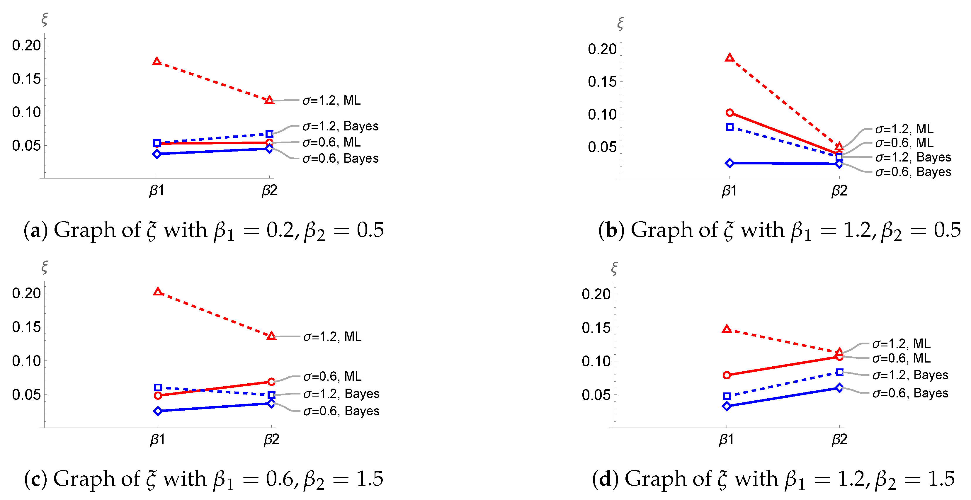
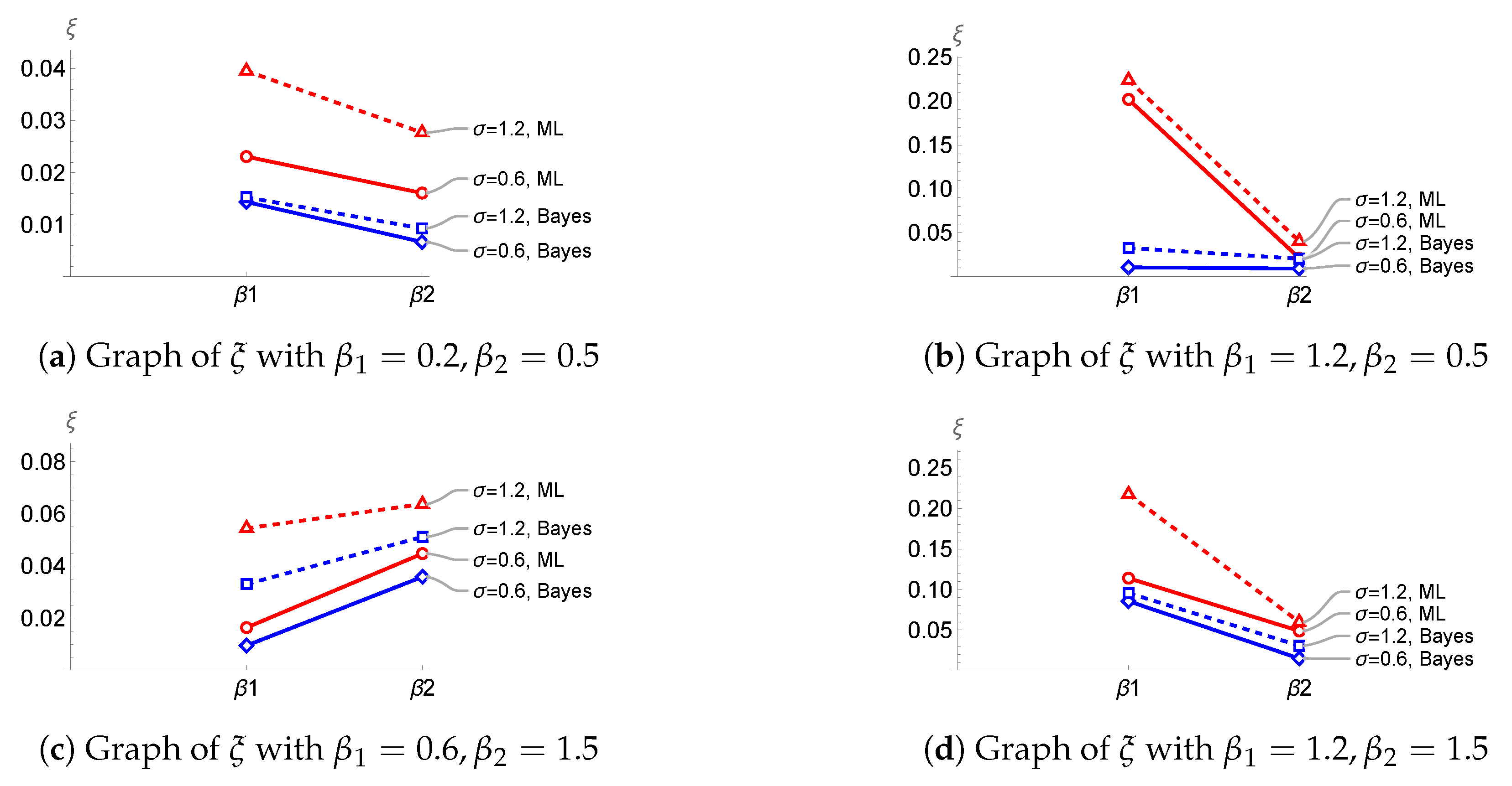
1.2	0.6013	(0.0263)	1.8275	(0.1922)	0.9343	(0.1802)	2.6341	(0.4903)	1.8447	(0.1514)	0.9349	(0.1560)	2.6180	(0.4114)

reveal that the ABC algorithm outperformed ML, as it had smaller ASE values. Additionally, for larger values of $\sigma$, which yielded extreme observations in the generated data, the ASE of the regression parameters increased for both the ABC and the ML estimates. Figure 3, Figure 4 and Figure 5, respectively, provide a visual summary of the numbers in Table 2, Table 3 and Table 4 and support the same conclusion. From an insurance industry perspective, a small ASE in regression parameters ensures highly accurate and stable predictions of insurance loss severity, which combines heavy-tailed extreme events with frequent small claims separated by a threshold. This minimizes volatility in capital allocation and premium pricing models. Most often, insurers rely on composite distributions such as LogNormal–Pareto to model both frequent, low-cost attritional losses and rare, catastrophic tail risks. A small ASE directly limits the variance of parameter estimates, preventing severe over- or underestimation of reserve requirements.

7. Goodness-of-Fit and Sensitivity Analysis

This section discusses the goodness of fit of the generated and real data sets to the LogNormal–Pareto composite distribution.

Table 5. Generated sample from LogNormal–Pareto (${\theta }_t=15$, ${\sigma }_t$ = 0.6).

4.16386	4.82515	5.6611	6.17322	6.90403	7.25687	7.27896	7.29432	7.43542	7.45443
7.53316	7.68981	7.74206	7.75907	8.23694	8.56252	9.13305	9.33552	10.0383	10.4195
10.4696	10.5193	10.8722	12.6541	12.6833	12.7263	13.1683	13.8473	14.3095	14.3217
14.5525	14.9635	14.991	15.4512	16.0533	16.4824	16.6144	16.8277	16.9492	17.3335
18.8477	20.1096	20.4049	20.7197	20.7957	22.1233	24.3231	25.0428	25.1696	26.2846
26.7286	26.7579	26.8502	28.9008	29.2378	29.3444	30.3729	30.3945	30.4302	31.3167
31.6275	31.9111	32.1681	34.9402	35.5428	38.538	39.4188	40.0925	43.4184	47.8926
47.923	48.3117	49.2027	51.4133	54.4194	63.1198	65.432	72.7723	73.3125	74.3392
100.284	119.793	122.711	135.812	138.105	138.803	145.339	171.228	213.533	242.595
308.472	434.651	527.658	563.648	652.523	774.342	833.14	1477.94	1908.15	2089.69

lists a generated sample of size 100 drawn from the LogNormal–Pareto. For this data set, using Code B, the MLEs are

$$\widehat{\sigma }=0.71,\widehat{\theta }=16.96,m=39.$$

The Anderson–Darling (AD) test is performed in Mathematica to assess the goodness of fit of a data set to the LogNormal–Pareto model, using the command: AndersonDarlingTest[y, f, “TestDataTable”]; y is the list of observations, and f is the piecewise PDF for the LogNormal–Pareto (4). We obtained AD = 0.3680 with a p-value = 0.879452, confirming that the data set fits the composite distribution well, as expected.

To demonstrate the computations involved in our proposed method for the regression model, we considered a real data set representing the total payment (y) for auto claims, in thousands of Swedish Kronor, available at https://www.kaggle.com/datasets/redwankarimsony/auto-insurance-in-sweden (accessed on 15 May 2026). We modified the data by adding five values $(601.2,820.1,1530.5,1930.5,2631.5)$ to y and x (# of claims) to obtain a better fit to the LogNormal–Pareto model; otherwise, the p-value for the AD test based on the original data set was 0.0390:

$$\begin{array}{c}y=\{4.4,6.6,11.8,12.6,13.2,14.6,14.8,15.7,20.9,21.3,23.5,27.9,31.9,32.1,38.1,39.6,39.9,40.3,46.2,48.7,48.8,\hfill \\ 50.9,52.1,55.6,56.9,57.2,58.1,59.6,65.3,69.2,73.4,76.1,77.5,77.5,87.4,89.9,92.6,93.,95.5,98.1,103.9,113,119.4,\hfill \\ 133.3,134.9,137.9,142.1,152.8,161.5,162.8,170.9,181.3,187.5,194.5,202.4,209.8,214.,217.6,244.6,248.1,392.5,\hfill \\ 422.2,601.2,820.1,1530.5,1930.5,2631.5\}\hfill \end{array}$$

$$x_1^{\prime }=\mathrm{the}\mathrm{vector}\mathrm{of}1’\mathrm{s}\mathrm{taking}\mathrm{into}\mathrm{account}\mathrm{the}\mathrm{intercept}\mathrm{in}\mathrm{the}\mathrm{regression}\mathrm{model}.$$

$$\begin{array}{ll}{x}_2^{\prime }=& \{3,2,4,4,3,6,6,13,5,11,11,7,13,15,4,23,13,5,19,9,7,6,9,18,23,11,12,16,10,25,41,8,7,14,19,13,\\ & 27,13,14,20,29,24,24,17,37,22,55,57,41,26,30,35,31,45,16,33,48,29,44,36,15,23,32,35\}\end{array}$$

Using Code B, we got

$$\widehat{\theta }=44.8571,\widehat{\sigma }=0.689201,m=19,n=67$$

and via Mathematica, AD = 1.8873, with p-value = 0.1062.

Goodness-of-fit (GOF) of the data set was also assessed for several composite distributions proposed in the literature. The MLEs of the corresponding parameters for each distribution were obtained, and BIC values and Anderson–Darling (AD) test p-values were computed. Although the BIC value for LogNormal was higher than Gamma–Pareto and InverseGamma–Pareto,

Table 6. GOF of composite models to the data set based on BIC and AD.

	LogNormal–Pareto	Exponential–Pareto	Gamma–Pareto	InverseGamma–Pareto
BIC	835.493	1185.13	402.434	766.853
AD test	1.8873	7.7756	21.4564	4.7602
AD-p-value	0.1062	0.0001	0.0000	0.0037
m	19	39	32	14

shows that the AD p-values for the Inverse-Gamma–Pareto, Exponential–Pareto, and Gamma–Pareto composite models were very small, indicating poor fit to the data. Based on the AD p-value, the LogNormal–Pareto model was a reasonable fit to the data set. It is worth mentioning that the Anderson–Darling (AD) test was more sensitive to the selected distribution. Unlike the Bayesian Information Criterion (BIC), which primarily penalizes model complexity to avoid overfitting, the AD test focuses exclusively on goodness of fit and places heavy weight on discrepancies in the tails of the distribution.

Consequently, at the 0.01 and 0.05 significance levels, the claim amount was concluded to follow the LogNormal–Pareto model.

As for the regression model, the MLEs for the parameters were

$${\widehat{\beta }}_0=1.3374,{\widehat{\beta }}_1=0.24915,$$

with

$$\mathrm{IFM}=\left[\begin{array}{cc}0.0273398& -0.002169\\ -0.002169& 0.000246772\end{array}\right],\mathrm{Wald}\mathrm{test}=(8.0884,15.8607).$$

(17)

The Wald test statistics indicate that the covariate (# of claims) is significant and that ${\beta }_0$ should be retained in the model.

In the context of regression analysis, using the significant covariate $x_1$ (the number of claims) in the model, $Va{R}_{(1-\gamma )}$ (see Section 2) can be computed. For example, with $(1-\gamma )=0.95,\widehat{\sigma }=0.689201(\alpha ={\displaystyle \frac{w}{\sigma }}=0.5401),\widehat{\theta }=e^{{\widehat{\beta }}_0+{\widehat{\beta }}_1{x}_1}$, and the number of claims $x_1=12$, we get $Va{R}_{\left(0.95\right)}=7724.05.$

Following the method proposed in the article, 1000 samples were generated from the multivariate Normal distribution with mean $\widehat{\beta }=(1.3374,0.24915)$ and the variance–covariance matrix, IFM in (17). The ABC-based estimates were computed as

$${\widehat{\beta }}_{0,Bayes}=1.33979,{\widehat{\beta }}_{1,Bayes}=0.250318,Na=426.$$

Code D (see the Supplementary Materials) provided computations for the ABC estimates of the regression parameters.

The original data, which excluded the last 5 numbers at the end of the vector y above and the last 5 rows of the design matrix X above, was also analyzed, and the results are given below.

$$\widehat{\theta }=43.5786,\widehat{\sigma }=0.586609,m=18,n=62$$

and via Mathematica, AD = 2.77657 with p-value = 0.035766. We can see that the original data did not fit the LogNormal–Pareto model as well as the modified data, as indicated by the smaller p-value. The parameter estimates differed slightly, and $m=18$. The MLEs for the parameters were

$${\widehat{\beta }}_0=1.35251,{\widehat{\beta }}_1=0.235205$$

with

$$\mathrm{IFM}=\left[\begin{array}{cc}0.025064& -0.002127\\ -0.002127& 0.000258\end{array}\right],\mathrm{Wald}\mathrm{test}=(8.5431,15.7428)$$

Note that the MLEs of the regression parameters and the FIM did not change drastically.

The ABC-based estimates were

$${\widehat{\beta }}_{0,Bayes}=1.38892,{\widehat{\beta }}_{1,Bayes}=0.248915,Na=520.$$

Sensitivity Analysis

In the following, the sensitivity of the proposed method was investigated with respect to the model assumption about the loss data.

1.

Instead of the LogNormal–Pareto model, the Exponential–Pareto model was considered for the original claim data with $n=62$ observations. The Exponential–Pareto composite model’s PDF is

$$f_Y\left(y\right)=\left\{\begin{array}{cc}{\displaystyle \frac{0.775}{\theta }}{e}^{{\displaystyle \frac{-1.35y}{\theta }}}\hfill & 0<y\le \theta \hfill \\ 0.2{\theta }^{35}{y}^{-1.35}\hfill & \theta \le y<\infty \hfill \end{array}\right.$$

Using the data and the algorithm given in Aminzadeh and Deng (2018), we obtained the MLE $\widehat{\theta }=77.1118$, $m=34$, and AD = 50.9115, with p-value = 0, indicating that the data did not fit the Exponential–Pareto model. Using the algorithm proposed in the current article, the MLEs for the regression parameters were computed as

$${\widehat{\beta }}_0=1.58439,{\widehat{\beta }}_1=-1.00246.$$

It is noted that ${\widehat{\beta }}_1$, in particular, was markedly different from its value under the LogNormal–Pareto model. In addition, the expected values, similar to (13), of the Exponential–Pareto model did not converge. As a result, the IFM could not be computed under the Exponential–Pareto model assumption. Therefore, the proposed method for computing ABC estimates of regression parameters could not be applied either. It is concluded that the requirements for applying the proposed ML and ABC methods are that the data should fit the composite model and that the expected values of the composite model should exist to apply ABC via IFM.

2.

A data set of size $n=300$ generated from the LogNormal–Pareto model was used to compute regression estimates based solely on the LogNormal PDF. The same link function ${\theta }_i=e^{x_i^{\prime }\beta }$ was used with $p=3$. The likelihood optimization did not converge, so the MLEs were not computable, implying that the proposed method in the article is sensitive to data characteristics and that the appropriate distributional model must be used.

• Summary

We introduced a nonlinear regression model using the LogNormal–Pareto composite distribution. From an insurance industry perspective, precise regression parameters yield highly accurate, stable predictions of insurance loss severity that combine heavy-tailed extreme events with frequent small claims, separated by a threshold. This minimizes volatility in capital allocation and premium pricing models. An exponential link function is proposed to compute MLEs and ABC-based estimates for regression parameters. Our approach provides closed-form formulas for the MLEs of the regression parameters in the cases with two and three covariates. Wald’s test statistic, based on the Fisher information matrix, is used to identify insignificant covariates. A multivariate normal distribution is used as the prior for the regression parameters, and its parameters are estimated via MLE. The Anderson–Darling goodness-of-fit test and the Bayesian information criterion (BIC) assess the fit between the response variable and the composite distribution. Our simulations confirmed that the ABC method outperforms the ML method, yielding lower ASE values. Simulated data from the LogNormal–Pareto distribution and a real-world data set were used as illustrative examples for computations. The computation of VaR was also illustrated in the context of regression modeling on the real data set. It was demonstrated that the proposed method was sensitive to the model assumption for the loss data. When incorrect distributions, such as Exponential–Pareto or LogNormal models, were applied to data generated by a LogNormal–Pareto model, they led to computational challenges for the MLEs of the regression parameters, as the likelihood function of the incorrect model failed to converge, rendering the MLEs infeasible. The choice of tolerance parameter for the ABC method is crucial. The selection of the tolerance parameters ${ϵ}_1$ and ${ϵ}_2$ for the application of the ABC method depends mainly on the available $y_1,y_2,\dots ,y_k$ and the simulated data based on generated regression parameter values from the posterior distribution. To better select the tolerance parameters, it is suggested to print a few values of the absolute differences between the percentiles to inform the appropriate choices for ${ϵ}_1$ and ${ϵ}_2$.

Potential future research involves modeling loss data using composite models and modeling the threshold parameter of the composite distribution via time-series models.