Article

Digital Financial Inclusion and Household Financial Fragility: Evidence of a U-Shaped Relationship in China


1
Faculty of Management and Economics, Kunming University of Science and Technology, Kunming 650031, China
2
School of Teacher Education, Dali University, Dali 671003, China
*
Author to whom correspondence should be addressed.
Risks 2026, 14(7), 164; https://doi.org/10.3390/risks14070164
Submission received: 26 May 2026 / Revised: 5 July 2026 / Accepted: 10 July 2026 / Published: 15 July 2026
(This article belongs to the Special Issue Digital Finance, Green Transition and Financial Risks)

Abstract

China’s rising household leverage has intensified concern about household-level financial risk, yet the role of digital financial inclusion (DFI) remains ambiguous. This study examines the association between DFI and household financial fragility through two channels: an information channel and a credit-constraint channel. We develop a three-period household decision framework and test its implications using China Family Panel Studies (CFPS) data from 2014 to 2022, matched with a county-level DFI index. The results show a U-shaped association between DFI and household financial fragility. Mechanism tests are consistent with a leverage channel: broader credit availability is associated with higher household leverage and higher distress risk. Evidence for the risk-taking channel is more conditional and becomes more visible at higher levels of DFI development. Instrumental-variable estimates, lagged specifications, alternative fragility measures, and double machine learning produce the same nonlinear sign pattern, although the exact turning point is specification-sensitive and the exclusion restriction remains an identifying assumption. The findings support risk-based monitoring of digital credit and consumer-protection policies targeted at households with weak liquidity buffers and high debt-service burdens.

1. Introduction

Household financial fragility is an important issue in applied risk research because fragile balance sheets can constrain consumption and amplify the effects of income shocks. Over the past decade, China’s household sector leverage has risen from 36% to 63.2% (Bank for International Settlements n.d.), making household balance sheets more sensitive to income volatility. During the same period, digital finance—including mobile payments, online credit, and digital wealth management—has changed how households access financial services. Although this expansion may improve financial inclusion by reducing transaction costs and broadening access, it may also raise concerns about debt sustainability (Zhang and Guo 2020; Fagereng et al. 2024; Song 2019). The net association between digital financial inclusion and household financial fragility, therefore, requires empirical assessment.
China provides a useful setting for studying this issue. Digital finance has expanded beyond conventional banking channels and now includes mobile payments, online consumer credit, digital wealth management and insurance (Wang and Meng 2025). This expansion is commonly viewed as a channel of financial inclusion, but it has occurred alongside a marked increase in household leverage. Whether these developments are connected, and through which mechanisms, remains an open question.
Existing research offers mixed conclusions. One strand emphasizes the inclusion channel: easier access to credit and payments may help households smooth consumption and manage shocks, thereby reducing financial vulnerability (Zhang et al. 2025; Chen et al. 2025). Another strand highlights the possibility that easier credit access and complex digital products may encourage excessive borrowing, speculative investment, or short-sighted financial decisions, thereby increasing the likelihood of distress (He et al. 2020; Lei et al. 2023). These views imply that digital finance may combine two mechanisms that work in different directions: an information effect and a credit-constraint effect.
We therefore model the DFI–fragility relationship as nonlinear. At relatively low levels of DFI, improved information access and lower transaction costs may reduce vulnerability by improving household financial choices. At higher levels, however, the expansion of digital credit and the increased salience of risky products may dominate, raising leverage and distress risk. The sign and magnitude of the relationship should therefore depend on the stage of local digital-finance development.
Estimating this nonlinear relationship requires attention to local economic shocks and reverse credit demand. We estimate two-way fixed-effects models using CFPS household panel data for 2014, 2016, 2018, 2020, and 2022, matched with a county-level DFI index. To mitigate endogeneity concerns, we use a Bartik-style instrumental-variable design that interacts predetermined telecommunication infrastructure and geographic deployment costs with aggregate internet diffusion. We further assess robustness using lagged DFI, alternative fragility measures, different fixed-effect structures, and double machine learning (DML).
Prior work has documented nonlinear effects of digital finance and credit-expansion channels separately, but typically treats the household information environment as exogenous and measures fragility with point-in-time, realized-distress indicators. Our advance is to make both the information environment and the borrowing limit endogenous functions of the same underlying variable—digital financial inclusion—so that the U shape emerges as an equilibrium property rather than as a reduced-form regularity, and to pair this with an ex ante, simulation-based fragility measure that operationalizes the model’s distress probability. This study contributes to the literature in three ways. First, it develops an intertemporal household model in which digital finance jointly shapes perceived risk (information effect) and feasible borrowing (constraint effect); the framework generates a testable prediction of a U-shaped relationship between DFI and financial fragility from primitives rather than by assumption. Second, it constructs a forward-looking, probability-based measure of household financial fragility. Using Monte Carlo simulations to introduce standardized income shocks, the indicator approximates the model’s concept of ex ante distress risk. Third, the paper provides identification-oriented evidence using a shift-share IV and examines how the relationship varies with the macro digital-finance environment, the traditional financial ecosystem, and household endowments.
The remainder of the paper proceeds as follows. Section 2 reviews the literature and develops the theoretical framework. Section 3 describes the data, variables, and identification strategy. Section 4 presents the baseline results, robustness checks, instrumental-variable analysis, and mechanism tests. Section 5 examines exposure heterogeneity. Section 6 concludes with policy implications and limitations.

2. Literature Review and Theoretical Framework

This study sits at the intersection of three fields: digital finance, household leverage, and financial fragility. This section reviews the relevant literature and develops the theoretical framework that motivates the empirical specification.

2.1. Literature Review

Research on the microeconomic effects of digital finance reaches mixed conclusions. One strand emphasizes its inclusive function, showing that broader access to digital financial services can ease credit constraints, smooth consumption, and promote entrepreneurship (Tao et al. 2023; Wu and Wu 2023; Zhang and Pang 2025). A second strand documents potential adverse consequences, linking easier credit access and complex digital products to over-indebtedness and increased volatility in household asset portfolios (Hu et al. 2024; Chen and Liu 2024; Liu and Zhang 2024). This divergence reflects two mechanisms of digital finance: an information effect that changes households’ information environment and risk perception, and a constraint effect that relaxes borrowing limits.
Although these two effects are widely recognized, studies often evaluate them in isolation, implicitly assuming a monotonic relationship—characterizing digital finance as either beneficial or detrimental (Tian 2022; Yang et al. 2025). However, the interaction between these effects is more likely to generate a dynamic, non-monotonic trajectory. At lower levels of market penetration, the inclusive benefits dominate: digital finance acts as a stabilizing force by easing traditional credit constraints and building household resilience (Fu 2024; Peng and Liu 2024; Qian et al. 2025). Yet, as the digital ecosystem matures, this stabilizing effect can reverse. Unrestricted access to digital credit eventually triggers the constraint effect, amplifying fragility by facilitating over-indebtedness and speculative risk-taking (Hu et al. 2024; Zhang and Zhang 2026). This U-shaped evolution reflects a structural shift from information-driven optimization to leverage-driven fragility, with the exact turning points heavily dependent on demographic and geographic endowments, such as urban–rural divides and aging (Liu et al. 2024; Wang and Mao 2023).
Parallel to the digital-finance literature, research on household financial fragility has traditionally focused on exogenous shocks—such as unemployment or health crises—as the primary drivers of insolvency (Akerlof et al. 2015; Zhou and Tian 2026). While recent behavioral studies provide micro-foundations for suboptimal borrowing driven by cognitive biases (Korteling et al. 2023; Lai and Gershman 2024; Simonse et al. 2024), they treat the household information environment as exogenously given. In reality, digital financial innovation fundamentally restructures the information households receive, thereby endogenously shaping their perceived uncertainty and subsequent risk-taking behavior. Existing frameworks rarely integrate this dynamic evolution of endogenous financial risk with traditional exogenous income shocks.
This theoretical limitation also affects empirical measurement. The literature typically operationalizes financial fragility through static indicators, such as contemporaneous debt-service burdens or liquidity shortfalls (Michelangeli and Rampazzi 2016; Ampudia et al. 2016). These point-in-time metrics describe realized distress but are less suited to measuring ex ante distress risk under uncertainty. Forward-looking measures that combine household balance-sheet conditions with simulated shocks are still relatively limited.
To address these gaps, this study develops an intertemporal decision model that incorporates exogenous income shocks, endogenous financial risk, and endogenous credit constraints. By specifying how the information and constraint effects jointly produce a U-shaped relationship, and by constructing a probability-based empirical indicator, the paper offers a framework for assessing the risk implications of digital financial inclusion.

2.2. Theoretical Framework: A Dynamic Model with Dual Uncertainties and Endogenous Credit Constraints

This section develops a parsimonious three-period household decision model to clarify how digital financial inclusion (DFI) affects household financial fragility. The model incorporates two sources of uncertainty: exogenous income shocks and endogenous financial risk generated by household portfolio and borrowing decisions. DFI affects the household through two channels. The first is an information channel, which changes perceived risk and risk-taking. The second is a credit-constraint channel, which changes the feasible borrowing set and debt-service burden. The model is not intended for structural estimation; its purpose is to derive testable comparative statics for the empirical analysis.

2.2.1. Model Setup

Consider a representative household that maximizes expected lifetime utility over three periods (t = 0, 1, 2):
V 0 = max c t , D 1 , α 1 E 0 t = 0 2 β t u c t ,   0   <   β   <   1
where C t denotes consumption and β is the discount factor. Period utility follows the CRRA form:
u ( c t ) = c t 1 γ 1 γ ,   γ   >   0
This function satisfies U =   C t γ   >   0 (positive marginal utility), U =   γ C t γ 1   <   0 (risk aversion), and U =   γ ( γ   +   1 ) C t γ 2   >   0 (prudence/precautionary savings motive), thereby providing the micro-foundation for analyzing behavior under uncertainty (Kimball 1990).
The household chooses first-period borrowing D 1 and allocates investable wealth A 1 between a risk-free asset and a risky asset. The risky asset share is denoted by α 1 [ 0 ,   1 ] . The risk-free return is r f , and the stochastic risky return is R 2 . The borrowing decision is subject to an endogenous credit constraint:
0     D 1     D - ( DFI ) , D - ( DFI )   >   0 ,
where D - ( DFI ) is the maximum borrowing limit. DFI also affects the borrowing cost:
r D   =   r D ( DFI ) , r D ( DFI )     0 .
Thus, higher DFI relaxes the borrowing constraint and may reduce the borrowing interest rate. However, whether it lowers financial fragility depends on the relative strength of the information and credit-expansion effects.

2.2.2. Dual Uncertainties and Financial Fragility

The household faces two sources of uncertainty in period t = 2.
First, income is subject to an exogenous shock:
Y 2   =   Y ̄ 2   +   ε Y ,   E ε Y   =   0 ,   Var ε Y   =   σ Y 2
Second, the household faces endogenous financial risk through its risky-asset allocation:
R 2   =   μ R +   ε R ,   E ε R   =   0 ,   Var ε R   =   σ R 2
Period-2 liquid resources are
L 2   =   Y 2   +   A 1 1     α 1 1   +   r f   +   α 1 1   +   R 2   E 2
where E 2 denotes necessary expenditure. The period-2 debt-service obligation is D S 2   =   [ 1   +   r D ( DFI ) ] D 1 .
A household is financially distressed if liquid resources are insufficient to cover debt-service obligations: L 2   <   D S 2 . Accordingly, theoretical household financial fragility is defined as the ex ante probability of distress:
P ( DFI )   = Pr ( L 2   <   D S 2 )
This theoretical object corresponds to the empirical forward-looking financial fragility indicator, fragility, constructed later through Monte Carlo simulations.

2.2.3. Information Channel: Perceived Risk and Risk-Taking

DFI changes the household’s information environment. At low levels of DFI, better access to information, lower search costs, and improved disclosure reduce uncertainty and improve portfolio decisions. At high levels of DFI, however, abundant platform information, recommendation algorithms, and salient short-term returns may cause households to underweight downside risk. To formalize this mechanism, let the household’s perceived risky-return variance be
σ ~ R 2 ( DFI )   =   σ R 2 m ( DFI ) ,   m ( DFI )   >   0
where m ( DFI ) is a misperception multiplier. When m ( DFI )   >   1 , the household overestimates risk and behaves too cautiously. When m ( DFI )   <   1 , the household underestimates risk and becomes overconfident.
To give m ( DFI ) a micro-foundation, suppose the household observes n ( DFI ) financial signals, where n DFI   >   0 .
Only a fraction a(DFI) ∈ (0, 1] of these signals is effectively processed because attention is limited. In addition, the processed information may be biased toward salient recent gains, captured by a distortion factor b(DFI) ∈ (0, 1]. We write
m ( DFI )   =   [ 1   + σ ν 2 a ( DFI ) n ( DFI ) σ R 2 ] b ( DFI )
where σ ν 2 measures signal noise. The bracketed term captures the precision effect: as DFI rises and more signals become available, perceived uncertainty falls toward the true variance. The term b ( DFI ) captures attention-driven distortion: as information becomes abundant and more salience-based, households may underweight tail risk.
Assume that m DFI   <   0 , and that there exists a cognitive threshold DFI ¯ such that m ( DFI ¯ )   =   1 .
Then
m ( DFI )   >   1 ,   DFI   <   DFI ¯ m ( DFI )   <   1 ,   DFI   >   DFI ¯
Under the standard mean-variance approximation to the CRRA portfolio problem, the optimal risky-asset share based on perceived risk is
α 1 * ( DFI )   = μ R r f γ σ ~ R 2 ( DFI )   =   μ R r f γ σ R 2 m ( DFI )
Let the benchmark allocation under correct risk perception be α 1 T = μ R r f γ σ R 2 .
Because m DFI   <   0 , we have α 1 * ( DFI ) DFI   >   0
However, the implication of this increase differs across DFI stages. When DFI   <   DFI ¯ , m ( DFI )   >   1 , so α 1 * ( DFI )   <   α 1 T .
In this case, the household overestimates risk and behaves too cautiously; higher DFI reduces this over-caution and moves the risky-asset share toward its benchmark level.
The fragility cost associated with risk misperception can be locally represented as
P info DFI   =   κ α 1 * DFI     α 1 T 2 ,   κ   >   0
Differentiating with respect to DFI gives
P info ( DFI ) DFI   =   2 κ α 1 * ( DFI ) α 1 T α 1 * ( DFI ) DFI
Because α 1 * ( DFI ) DFI   >   0 , the sign of the information channel depends on whether perceived risk is above or below true risk:
P info DFI DFI   <   0   if   DFI   <   DFI ¯ P info DFI DFI   >   0   if   DFI   >   DFI ¯
Thus, the information channel is non-monotonic. At low DFI levels, it reduces fragility by improving risk perception and allocation. At high DFI levels, it may increase fragility by encouraging excessive risk-taking.

2.2.4. Credit-Constraint Channel: Borrowing Capacity and Leverage

DFI also affects household fragility through the borrowing constraint. When the credit constraint binds, the household borrows up to the available limit: D 1   * =   D ̄ ( DFI ) .
The corresponding debt-service obligation is
D S 2 ( DFI )   =   [ 1   +   r D ( DFI ) D ̄ ( DFI ) ]  
Differentiating gives
D S 2 DFI DFI   =   1   +   r D DFI D ̄ DFI   +   D ̄ DFI r D DFI
Although r D DFI 0 , DFI raises the borrowing limit. The credit-expansion effect dominates when
[ 1   +   r D ( DFI ) ] D ̄ ( DFI )   >   D ̄ ( DFI ) r D ( DFI )
Under this condition, D S 2 ( DFI ) DFI   >   0
Let F L ( ) and f L ( ) denote the cumulative distribution function and probability density function of L 2 . Since
P credit DFI   = Pr L 2   <   D S 2 DFI =   F L D S 2 DFI
we obtain P credit DFI DFI   =   f L D S 2 DFI D S 2 DFI DFI .
Because f L ( )   >   0 , Equation (17) implies P credit DFI DFI   >   0 .
Therefore, the credit-constraint channel monotonically increases financial fragility when credit expansion dominates the reduction in borrowing cost. Empirically, this channel corresponds to the leverage proxy debt asset.

2.2.5. Net Effect and Propositions

The total effect of DFI on household financial fragility can be decomposed into the information channel and the credit-constraint channel:
P ( DFI )   =   P 0   +   P info ( DFI )   +   P credit ( DFI )
where P 0 captures baseline fragility unrelated to DFI. Differentiating gives
P ( DFI ) DFI = P info ( DFI ) DFI + P credit ( DFI ) DFI
At low levels of DFI,
P info DFI DFI   <   0 ,   P credit DFI DFI   >   0
If the information-improvement effect dominates the credit-expansion effect, then
P info ( DFI ) DFI > P credit ( DFI ) DFI
which implies
P ( DFI ) DFI   <   0
At high levels of DFI, the information channel turns positive because risk underestimation and overconfidence become more relevant:
P info DFI DFI   >   0 ,   P credit DFI DFI   >   0
Therefore,
P ( DFI ) DFI   >   0
If P ( DFI ) is continuous and differentiable, Equations (22) and (23) imply the existence of an interior turning point DFI * such that
P ( DFI ) DFI DFI = DFI *   =   0
This delivers a U-shaped relationship between DFI and household financial fragility.
The theoretical framework yields three propositions.
Proposition 1. 
Non-monotonic information channel.
DFI affects financial fragility through perceived risk and risk-taking. At low levels of DFI, improved information reduces fragility by correcting excessive caution and improving allocation. At high levels of DFI, risk underestimation and overconfidence may increase risk-taking and raise fragility. Empirically, this mechanism is examined through the risk asset.
Proposition 2. 
Credit-constraint channel.
When credit expansion dominates the reduction in borrowing costs, DFI raises debt-service exposure and increases financial fragility through higher leverage. Empirically, this mechanism is examined through the debt asset.
Proposition 3. 
U-shaped net relationship.
The net effect of DFI on household financial fragility reflects the trade-off between the information channel and the credit-constraint channel. At low DFI levels, the negative information effect may dominate; at high DFI levels, the positive credit-constraint effect and overconfidence-related risk-taking effect dominate. Therefore, DFI and household financial fragility follow a U-shaped relationship.

3. Research Design

Building on the theoretical framework, we use CFPS household panel data matched with the county-level DFI index to test the predicted U-shaped relationship.

3.1. Data

The household data come from the 2014, 2016, 2018, 2020, and 2022 waves of the China Family Panel Studies (CFPS), a nationally representative longitudinal survey administered by Peking University (Xie and Hu 2014). The survey provides household-level information on demographics, income, assets, liabilities, and financial behavior.
DFI is measured using the Peking University Digital Financial Inclusion Index of China (PKU-DFIIC), compiled by the Institute of Digital Finance, Peking University and its collaborating research team (Guo et al. 2020). The index is available at provincial, prefecture-city, and county levels and includes three sub-dimensions: coverage breadth, usage depth, and digitization level. We match the county-level index to the CFPS county/district identifiers.
The cleaning procedure retains households with adult household heads, removes observations with missing or internally inconsistent key variables, and winsorizes continuous variables at the 1st and 99th percentiles. The final dataset is an unbalanced household-year panel. Because household balance-sheet variables are survey-based, measurement error—especially in informal or platform-based borrowing—is treated as a limitation and addressed through robustness checks where possible.

3.2. Variable Definitions

3.2.1. Main Variables

Dependent variables: Using the definition of financial distress as the risk that a household’s liquid assets are insufficient to meet its debts and incorporating adverse shocks, we construct two key indicators. (i) Forward financial fragility prediction indicator (fragility): This variable directly estimates the probability that a household will fall into financial distress, consistent with the theoretical model. (ii) Financial fragility dummy (Finsm): Following Michelangeli and Rampazzi (2016), a household in a survey year is classified as financially fragile (Finsm = 1) if it meets both of the following conditions: high debt-service burden, debt repayment/total household income > 30%; and low liquidity buffer, total household financial assets < total household liabilities. Otherwise, Finsm = 0.
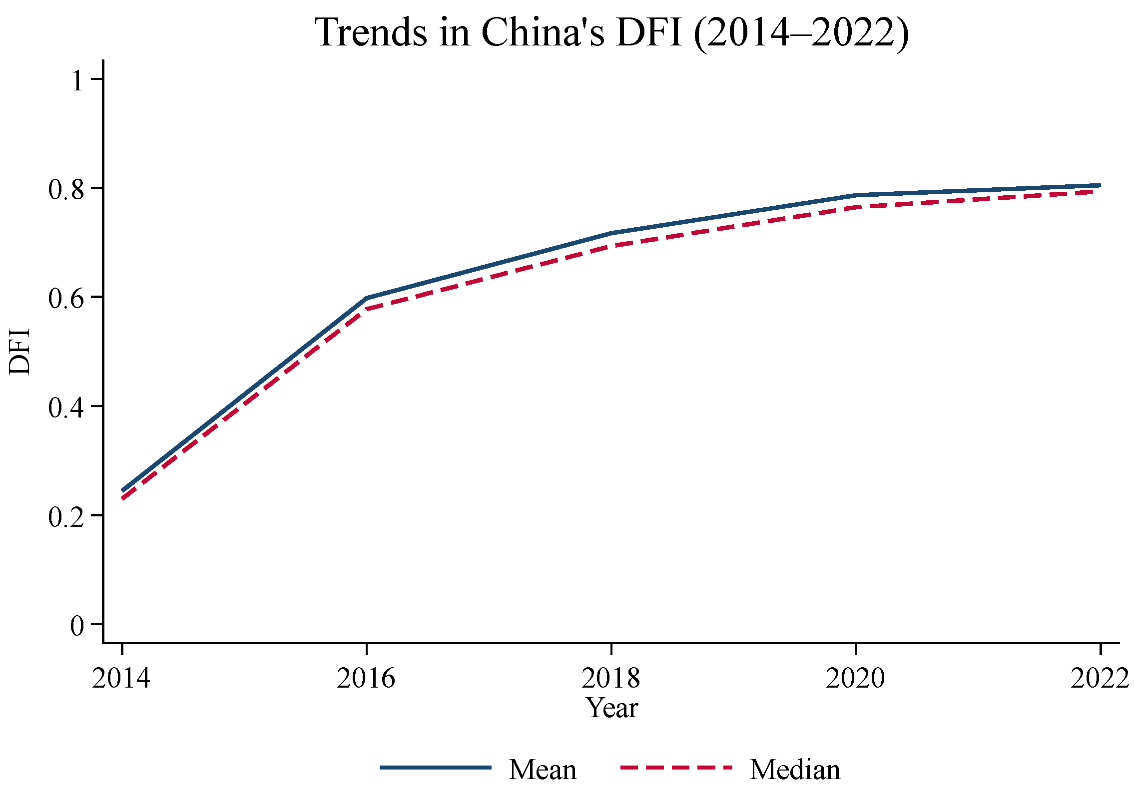
Core explanatory variable: DFI denotes the county-level Peking University Digital Financial Inclusion Index, rescaled to the interval [0, 1]. The empirical specification includes both DFI and DFI squared to test the nonlinear prediction in Proposition 3. Figure 1 shows the trend in China’s DFI from 2014 to 2022.
Mechanism Variables
Information-channel proxy: We use risky-asset allocation, risk asset, defined as the share of risky financial assets—stocks, funds, wealth-management products, and related instruments—in total financial assets. This proxy captures a revealed risk-taking margin; it cannot directly observe perceived variance and is therefore interpreted cautiously.
Credit-constraint proxy: We use household leverage, debt asset, defined as total household debt divided by total assets. This variable captures the balance-sheet consequence of relaxed borrowing constraints.
Control variables: Following the household-finance literature (Campbell 2006; Fort et al. 2016; Lusardi and Mitchell 2014), we control for household-head age, gender, education, marital status, health, hukou status, homeownership, log household per capita income, and fixed effects. These covariates reduce confounding from household capability, economic status, and local institutional conditions.

3.2.2. Construction of the Forward-Looking Financial Fragility Indicator (Fragility)

We develop a forward-looking financial fragility indicator to address the static limitations of conventional measures. By introducing a dynamic assessment mechanism for future uncertain shocks, the indicator links the theoretical concept of financial distress probability with an empirically operational measure. We construct a forward-looking measure of household financial fragility that operationalises the model’s concept of ex ante distress probability. The construction proceeds in four steps: (i) define financial distress as a state in which liquid resources are insufficient to meet debt obligations under adverse shocks; (ii) specify the key dimensions that govern distress risk—solvency, debt-servicing capacity, and income-shock sensitivity; (iii) calibrate parameters using a combination of prior evidence and conservative benchmarks; and (iv) implement household-level Monte Carlo simulations to obtain, for each household-year, the simulated frequency of distress events. The resulting variable, fragility , is interpreted as an estimated probability of distress over the simulation horizon and is therefore directly comparable across households and over time.
This indicator draws on three theoretical foundations in modern household finance. Modigliani’s Life Cycle–Permanent Income Hypothesis (Modigliani and Brumberg 1954) provides the intertemporal budget framework, suggesting that financial health cannot be assessed from a single-period perspective. Leland’s Precautionary Savings Theory (Leland 1968) explains why households hold liquid assets under uncertainty, motivating the inclusion of liquidity buffers. Diamond’s Liquidity Constraints Theory (Diamond and Kashyap 2016) underscores the role of debt-servicing capacity and liquidity buffers in financial stability, which we adapt to the household balance sheet. Together, these theories inform the indicator’s three dimensions: solvency crisis, debt sustainability, and income-shock sensitivity.
To make the procedure fully reproducible, we state the aggregate risk score explicitly. For household i in simulation draws, the composite risk score is a convex combination of three sub-scores,
R ( i , s )   =   w solv   ·   S solv   +   w sust   ·   S sust   +   w sens   ·   S sens
with non-negative weights w solv   =   0.4 , w sust   =   0.3 , and w sens   =   0.3 that sum to one. Each sub-score is bounded in [0, 1]. The solvency sub-score is S solv = max 0 , min 1 , 1 LC ( i , s ) 1.3 , where the liquidity-coverage ratio LC ( i , s ) = L i + Y ( i , s ) E i max ( D S i , 0.001 ) divides post-shock liquid resources—liquid assets L i plus realized income Y ( i , s ) net of basic expenditure E i —by the debt-service obligation D S i . The sustainability sub-score is S sust = min 1 , DTI ( i , s ) 0.30 , where DTI ( i , s )   =   D S i max ( Y ( i , s ) , 1 ) is the post-shock debt-service-to-income ratio. The sensitivity sub-score S sens is a step function of the realized income decline interacted with a high-leverage indicator (debt-to-asset ratio > 0.5): it equals 0.8 when income falls by at least 50% under high leverage, 0.5 when income falls by at least 30% under high leverage, 0.2 when income falls by at least 30% otherwise, and 0 elsewhere. A household is classified as distressed in draws when R ( i , s )   >   0.25 , and the fragility index is the share of distressed draws over S = 1000 simulations. Calibrated values follow the implementation: the liquid-asset ratio is 0.18 of income, the debt interest rate is 0.08, basic expenditure is 0.5 of income, and the income-shock standard deviation is 0.25. Crucially, the validation target—the contemporaneous distress dummy Finsm, defined from the debt-service burden and the liquidity buffer—is computed from balance-sheet ratios that do not enter the simulated score through the same functional form, so the concordance reported below reflects genuine predictive overlap.
The indicator has a mean of 0.016 and a standard deviation of 0.106. Its distribution is right-skewed (skewness = 8.189) and leptokurtic (kurtosis = 71.749), implying that most households display low financial fragility, while a small number exhibit very high fragility. Table 1 shows the risk-grade distribution: 87.39% of households are in the extremely low risk, 9.58% are low risk, 1.60% are medium risk, 0.23% are high risk, and 1.19% are very high risk.
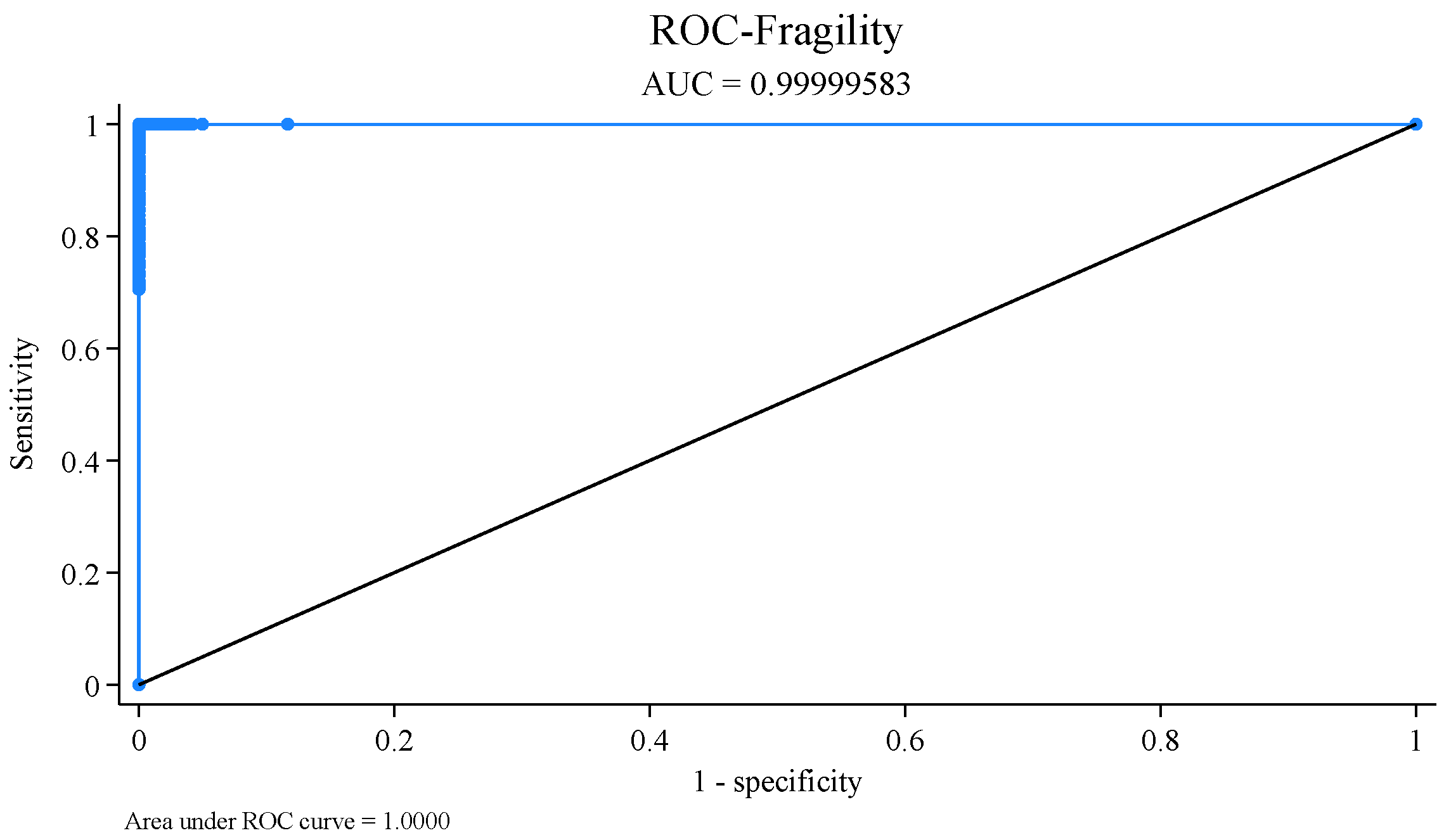
Validity checks show that this indicator is correlated with the contemporaneous financial fragility dummy (r = 0.928) and the debt-to-income ratio (r = 0.471), demonstrating its validity. By construction, this simulated measure highly correlates with contemporaneous default indicators, providing a theoretically consistent proxy for ex ante distress probability under standard shock assumptions (Figure 2). The measure exhibits high concordance with contemporaneous indicators; we interpret this as supportive evidence for validity. Performance comparisons across thresholds (Table 2) further confirm the indicator’s robustness.
Two features of the design guard against the concern that high concordance simply reproduces the validation target. First, the simulated index and the contemporaneous dummy are constructed from distinct functional mappings: the dummy is a deterministic threshold rule on two observed ratios, whereas the index aggregates three sub-scores over a thousand stochastic income draws, so the two need not coincide ex ante. Second, the index is not estimated by fitting to the dummy—no parameter is chosen to maximize in-sample classification—so the standard overfitting channel, in which flexible models memorize labels, does not apply. To probe predictive stability rather than mechanical fit, we split the panel by survey wave (training: 2014–2018; test: 2020–2022) and find that out-of-sample classification accuracy remains close to the full-sample figure, indicating that the concordance is not an artifact of in-sample tuning.
In the empirical analysis, fragility is used as a continuous stress-test measure. Because its level depends on calibrated shock distributions, weights, and thresholds, the paper emphasizes the sign and curvature of the DFI–fragility relationship rather than the absolute level of the simulated probability.

3.3. Empirical Strategy

We adopt a comprehensive empirical strategy comprising baseline regressions, mechanism tests, heterogeneity analysis, and endogeneity treatment. All models control for county fixed effects and year fixed effects to absorb time-invariant regional characteristics and common time trends. Standard errors are clustered at the county level.

3.3.1. Baseline Regression Model: Testing the U-Shaped Relationship

To test Proposition 3, we estimate the following two-way fixed-effects specification:
fragility it =   α   +   β 1 DFI it   +   β 2 DFI it 2   +   γ X it   +   λ c   +   μ t   +   ϵ it
where i and t denote household and year, respectively. fragility it is the dependent variable, including our constructed forward-looking indicator fragility, and the dummy variable Finsm is used for robustness checks. DFI it and DFI it 2 are the core explanatory variables, and their coefficients β 1 and β 2 are the focus. If β 1 is significantly negative and β 2 is significantly positive, it supports the U-shaped relationship hypothesis. X it is a vector of household and control variables. λ c and μ t are county and year fixed effects, respectively, controlling for time-invariant regional characteristics and common time-varying trends. ϵ it is the random error term.

3.3.2. Robustness Check: Double Machine Learning

As a robustness check, we implement double machine learning (DML) following Chernozhukov et al. (2018). DML is used to reduce specification bias by flexibly partialling out high-dimensional controls and nonlinear confounding patterns before estimating the orthogonalized association between DFI, DFI 2 , and financial fragility.
Let D it   =   DFI ct , DFI ct 2 denote the two-dimensional treatment vector and X it the vector of controls and fixed-effect transformations. We consider the partially linear model
fragility it   =   θ D it   +   g ( X it ) +   u it
For each fold k in a K-fold cross-fitting procedure, the nuisance functions are trained outside fold k and predicted inside fold k:
E [ fragility it X it ]   =   g y ( X it ) , E [ D j , it X it ]   =   g j ( X it ) ,   j   =   1 ,   2
The residualized variables are
fragility ~ it   =   fragility it g ^ y X it , D ˜ j , i t = D j , i t g ^ j X i t , j = 1 ,   2
The final stage estimates
fragility ~ it   =   θ 1 D ~ 1 , it   +   θ 2 D ~ 2 , it   +   η it
Equation (31) uses county-clustered standard errors. The DML exercise is treated as a robustness check for functional-form and control-flexibility concerns, not as a source of a sharper turning-point estimate.

3.3.3. Mechanism Test

To test the two transmission channels underlying Propositions 1 and 2, we estimate nonlinear mediation-style regressions for risk assets and debt assets. The model is specified as follows:
M it   =   a 0   +   a 1 DFI it   +   a 2 DFI it 2   +   a 3 X it   +   λ c   +   μ t   +   u it
Fragility it   =   b 0   +   b 1 DFI it   +     b 2 DFI it 2 +   τ M it   +   b 3 X it   +   λ c   +   μ t   +   v it
The parameters in Equation (32) measure the association between DFI and the mechanism variable, allowing for nonlinearity. The parameter on the mechanism variable in Equation (33) measures whether the mechanism is associated with financial fragility after controlling for DFI, DFI squared, controls, and fixed effects.

4. Empirical Results and Analysis

4.1. Descriptive Statistics and Preliminary Analysis

Table 3 presents descriptive statistics for all variables used in this study. The dependent variable, financial fragility, has a mean of 0.016. The core independent variable (DFI) has a mean of 0.632 and a standard deviation of 0.209, indicating considerable variation in DFI development across counties. Household-head characteristics show an average of 7.7 years of education and an average self-rated health of 3.12 (between fair and healthy). Married heads account for 85.5% of the sample, and male heads represent 52.3%. At the household level, 87.6% of households own their home, and the mean of the log of household per capita income is 2.155. Regionally, the urban–rural hukou distribution is relatively balanced, with urban hukou representing 47.9%.
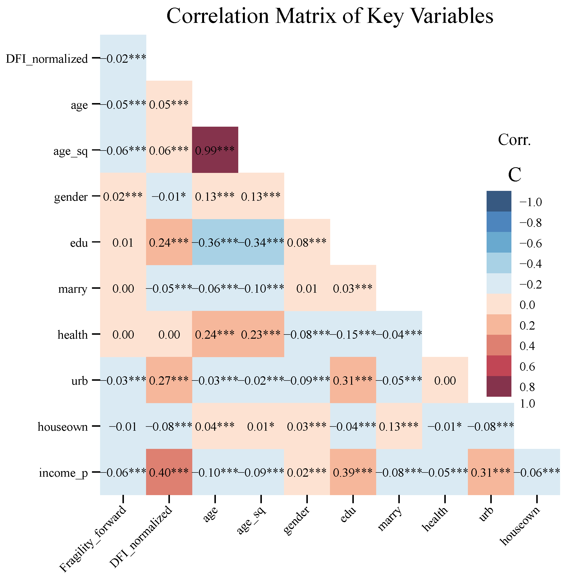
The correlation heatmap in Figure 3 shows that DFI has only a weak linear correlation with fragility. This is consistent with the possibility that a simple correlation may miss nonlinear patterns. All reported pairwise correlations are moderate in magnitude, suggesting that severe multicollinearity among the listed variables is unlikely.

4.2. Baseline Regression Results: The U-Shaped Relationship Between Digital Finance and Financial Fragility

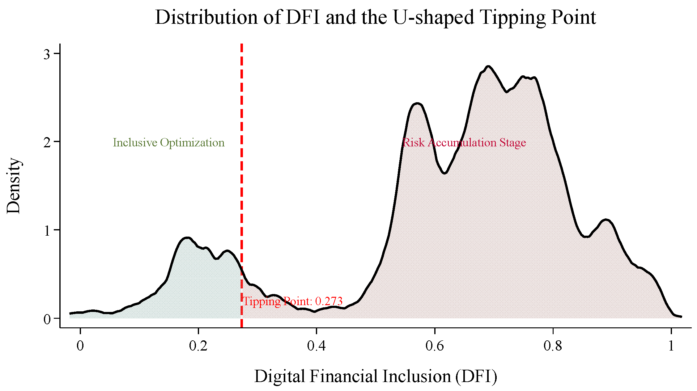
Table 4 reports the baseline results. Models (1) and (2), which include only the linear DFI term, show no statistically meaningful linear association. Models (3) and (4) add DFI squared and reveal the predicted nonlinear pattern. In Model (4), the linear coefficient is −0.052 (p < 0.1) and the quadratic coefficient is 0.095 (p < 0.01), implying a turning point of approximately 0.273. At the sample mean of DFI (0.632), the estimated marginal effect is positive. The implied effect size is economically nontrivial relative to the low mean of simulated fragility, but it should be interpreted as a change in predicted distress probability under the model’s scaling rather than as an observed default rate.
The estimated turning point should be interpreted as a risk-warning band, not as a deterministic policy cutoff. The point estimate lies below the sample mean, indicating that many observed county-years fall on the risk-accumulation side of the fitted curve. However, measurement error in informal and digital borrowing, as well as specification differences across robustness checks, may affect the exact location of the turning point.
Figure 4 overlays the estimated turning point on the kernel density distribution of DFI. The density plot indicates that a substantial share of observations lies to the right of the estimated threshold. This supports the interpretation that the risk-accumulation side of DFI is empirically relevant in the sample, while still leaving the exact threshold subject to estimation uncertainty.
The estimated inflection point may be affected by data quality. The household-head respondent is about 53 years old on average, and some respondents may underreport consumer or business loans obtained through emerging digital channels. Such underreporting would tend to lower measured financial vulnerability and could shift the estimated turning point. This issue motivates the cautionary interpretation of the threshold and is discussed further in the limitations section.
Overall, the baseline estimates indicate that the relationship between DFI and household financial fragility is not well described by a single linear coefficient. At lower levels of DFI, the association is negative; at higher levels, it becomes positive. This pattern is consistent with the theoretical trade-off between an information channel that can improve household decisions and a credit-constraint channel that can raise leverage and exposure to shocks.

4.3. Robustness Checks

We assess robustness along three dimensions: outlier treatment, alternative measurement and timing of key variables, and alternative estimation methods. The main emphasis is on the stability of the coefficient signs and the implied nonlinear shape; the exact turning point is expected to vary across specifications because it is a ratio of two estimated coefficients.

4.3.1. Addressing the Influence of Outliers

After winsorizing continuous variables at the 1st and 99th percentiles, column (1) of Table 5 shows that the linear and quadratic DFI coefficients remain negative and positive, respectively. The implied turning point is 0.283, close to the baseline estimate. This reduces concern that the U-shaped pattern is driven by extreme observations.

4.3.2. Changing Core Explanatory Variables

We conduct two robustness checks to address concerns about measurement choices for key variables and potential reverse causality.
Replacing the forward-looking fragility measure with the contemporaneous binary indicator Finsm preserves the U-shaped pattern (column 2) of Table 5. The estimated turning point rises to 0.382, which indicates that the level at which fragility begins to increase depends partly on whether fragility is measured as an ex ante probability or a contemporaneous distress state.
Using a one-period lag of DFI reduces contemporaneous reverse-causality concerns (column 3) of Table 5. The lagged specification again produces a negative-linear term, a positive-quadratic term, and a turning point of 0.315.

4.3.3. Adjusting Model Specification and Estimation Methods

This study further assesses how model specification affects the results by conducting two sensitivity tests.
Changing the fixed-effects structure shifts the estimated turning point more noticeably. As reported in column (4) of Table 5, with county fixed effects, the turning point is 0.137, while the signs of the DFI terms remain consistent with the U-shaped prediction. This sensitivity is expected because county and household fixed effects identify different sources of variation.
Column (5) of Table 5 shows that adding region-specific time trends also preserves the negative-linear/positive-quadratic pattern, with a turning point of 0.239. These specifications indicate that heterogeneous regional trends do not explain away the nonlinear relationship.

4.3.4. Double Machine Learning

The DML estimates in Table 5, column (6) preserve the negative-linear/positive-quadratic sign pattern: the linear DFI coefficient is −0.102 (p < 0.01), and the quadratic coefficient is 0.063 (p < 0.05). The implied turning point is 0.800, which is substantially higher than in the fixed-effects specifications. This difference should not be overinterpreted; the DML exercise changes the residualized variation used for estimation and is designed to probe functional-form robustness, not to deliver a sharper policy threshold.

4.4. Endogeneity and Instrumental Variables

Our instrumental-variable strategy follows the shift-share (Bartik) logic, in which predetermined local exposure is interacted with an aggregate diffusion process to generate plausibly exogenous variation (Goldsmith-Pinkham et al. 2020; Borusyak et al. 2022). The design uses historical communication infrastructure and terrain-related deployment costs to predict differential DFI growth as national internet penetration expands.
Let Tel c , 1984 denote the number of landline telephones per 100 people in county c in 1984. This variable captures pre-digital communication infrastructure and organizational capacity that plausibly affects the local cost of adopting digital financial services once nationwide digital technologies diffuse. Let Internet t denote the national internet penetration rate in year t, which proxies for aggregate technology diffusion common to all countries. Let Rugged c denote terrain ruggedness, which affects the physical cost of infrastructure deployment.
We construct three instruments:
Z ct ( 1 )   =   Tel c , 1984   ×   δ t Z ct ( 2 )   =   Tel c , 1984   ×   Internet t Z ct ( 3 )   =   Tel c , 1984   ×   Rugged c   ×   Internet t
where δ t denotes year indicators. The first instrument allows counties with different pre-existing communication infrastructure to exhibit different slopes in digital-finance diffusion across years; the latter two explicitly anchor identification on an aggregate diffusion process ( Internet t ) and predetermined local cost shifters ( Tel c , 1984 , Rugged c ).
(i) 
First stage and second stage
We estimate the first stage at the county–year level:
DFI ct   =   π 0   +   π 1 Z ct ( 1 )   +   π 2 Z ct ( 2 )   +   π 3 Z ct ( 3 )   +   ρ W ct   +   μ c   +   λ t   +   u ct
where μ c and λ t are county and year fixed effects, and W ct contains time-varying county controls when available.
The second stage follows the baseline quadratic specification at the household level:
fragility ict   =   β 0   +   β 1 DFI ^ ct   +   β 2 DF I ct 2 ^   +   γ X ict   +   μ c   +   λ t   +   ε ict
Because the model includes a nonlinear function of an endogenous regressor, we treat both DFI ct and DFI ct 2 as endogenous. In implementation, we instrument the vector ( DFI ct , DFI ct 2 ) using a standard 2SLS approach with a rich instrument set formed from { Z ct ( k ) } and their nonlinear transformations (e.g., squares and cross-products), which ensures identification of both the level and curvature terms while preserving the fixed-effects structure.
(ii) 
Identification discussion
The identifying assumption is that, conditional on county and year fixed effects, the interaction between historical infrastructure (or geography) and aggregate internet diffusion affects household financial fragility only through its impact on local DFI.
Following Goldsmith-Pinkham et al. (2020), our identification relies on the exogeneity of differential exposures to a common diffusion process. Crucially, any direct effects of historical communication capacity ( Tel c , 1984 ) or terrain ruggedness ( Rugged c ) on contemporary household balance sheets are absorbed by county fixed effects. Therefore, the exclusion restriction holds provided that unobserved time-varying regional shocks are uncorrelated with the initial local infrastructure setup.
A potential threat to this design is that counties with different historical infrastructure endowments might follow diverging economic trajectories correlated with household fragility—for instance, if 1984 telephone density proxies for persistent development that independently affects balance sheets. Three features address this concern. First, the level of historical infrastructure does not identify our parameter: because 1984 telephone density is time-invariant, its direct effect on fragility is absorbed by county fixed effects, and identification comes only from the interaction between that predetermined density and the aggregate, nationally common diffusion of internet penetration. The exclusion restriction, therefore, requires not that historical telecommunications be unrelated to development, but the weaker condition that its differential interaction with nationwide diffusion affects fragility solely through contemporary DFI. Second, to probe the residual concern that high- and low-infrastructure counties were already on different paths, our robustness checks add urbanization-by-year interactions, absorbing heterogeneous regional trajectories; the nonlinear pattern is unchanged. Third, the over-identification test does not reject the joint validity of the instrument set (p = 0.934), which would be unlikely if the instruments shared a common violation of the exclusion restriction. We nonetheless treat the exclusion restriction as an identifying assumption rather than a proven fact, and we flag quasi-experimental designs based on digital-finance regulation as a complementary identification strategy in the conclusion.
(iii) 
Diagnostics and main findings
Table 6 reports IV diagnostics and estimates. The first-stage statistics are above conventional weak-instrument thresholds, and the over-identification test does not reject the instrument set. The IV estimates are consistent with the U-shaped sign pattern, and the IV-implied turning point is 0.523. Because the exclusion restriction remains an identifying assumption, the results are presented as supportive, not conclusive, causal evidence.

4.5. Mechanism Tests

This section examines two channels through which DFI may influence household financial fragility: the information channel and the credit-constraint channel. The information channel is proxied by risky-asset allocation, while the credit-constraint channel is proxied by household leverage.

4.5.1. Information Channel: Risk-Taking

The theoretical model links the information channel to perceived risk and decision quality. CFPS does not directly observe perceived variance, so the risk asset is used as an indirect proxy for risk-taking. This variable captures whether households allocate a larger share of financial wealth to risky assets, but cannot distinguish rational diversification from overconfidence or risk misperception.
Columns (1) of Table 7 show a statistically significant U-shaped association between DFI and risk asset, with a turning point of 0.423. The evidence is therefore consistent with the information-channel mechanism, but weaker than the leverage-channel evidence.
Before the risk asset turning point, the risky-asset share declines or increases only slowly, which is consistent with better information reducing poorly informed investment. After the turning point, risk assets rise and are associated with higher fragility, consistent with information overload, product complexity, or overconfidence becoming more relevant in mature digital-finance environments.
This interpretation should remain cautious. The risky-asset share bundles rational and biased risk-taking, and the regression does not observe households’ subjective beliefs. Direct measurement of perceived risk, financial literacy, product understanding, and platform recommendation exposure would be required to separate these mechanisms more sharply.

4.5.2. Credit-Constraint Channel: Leverage

The credit-constraint channel is stronger and more stable. Table 7 shows that DFI is positively associated with household leverage over the observed support of DFI, and Table 8 shows that leverage is positively associated with financial fragility on both sides of the IV-estimated turning point. This pattern supports Proposition 2: DFI can raise fragility by expanding feasible borrowing and increasing household balance-sheet exposure.
Given the nonlinear relationship in the full sample, we conduct subgroup tests based on the turning point (DFI = 0.523) identified by the instrumental-variable regression. The results are shown in Table 8.
The split-sample analysis in Table 8 reinforces this interpretation. The risk-taking channel is not detected below the IV turning point but becomes positive above it. The leverage channel remains significant on both sides of the turning point, indicating that credit expansion is the more robust transmission mechanism. The smaller leverage coefficient above the turning point may reflect compositional differences or higher baseline leverage in mature DFI regions.

5. Exposure Heterogeneity in the DFI–Fragility Curve

The baseline estimates identify an average U-shaped relationship between DFI and household financial fragility. This section asks whether the shape of that curve differs across households. The exercise is not a second identification strategy. It is a boundary test of the mechanism: if the risk-accumulation side of the curve is driven by digital product exposure, risk misperception, and easier borrowing, it should be more visible among households with greater contact with digital financial markets.
The main text focuses on the urban–rural split because this dimension is closest to the mechanism. The information channel depends on digital capability, product familiarity, and the ability to process financial information. The credit-constraint channel depends on actual access to online credit and related products. These margins differ more directly across urban and rural households than across broad regional splits. The macro DFI environment and traditional-finance density are reported in Appendix A as transparency checks.
Table 9 reports shape-based heterogeneity tests. Panel A shows group-specific quadratic profiles, including the DFI coefficients, turning points, and Lind-Mehlum-style U-shape test within the observed support. This avoids interpreting the sign pattern of the linear and quadratic terms as sufficient evidence of a U-shaped relationship. Panel B tests whether the urban and rural profiles differ.
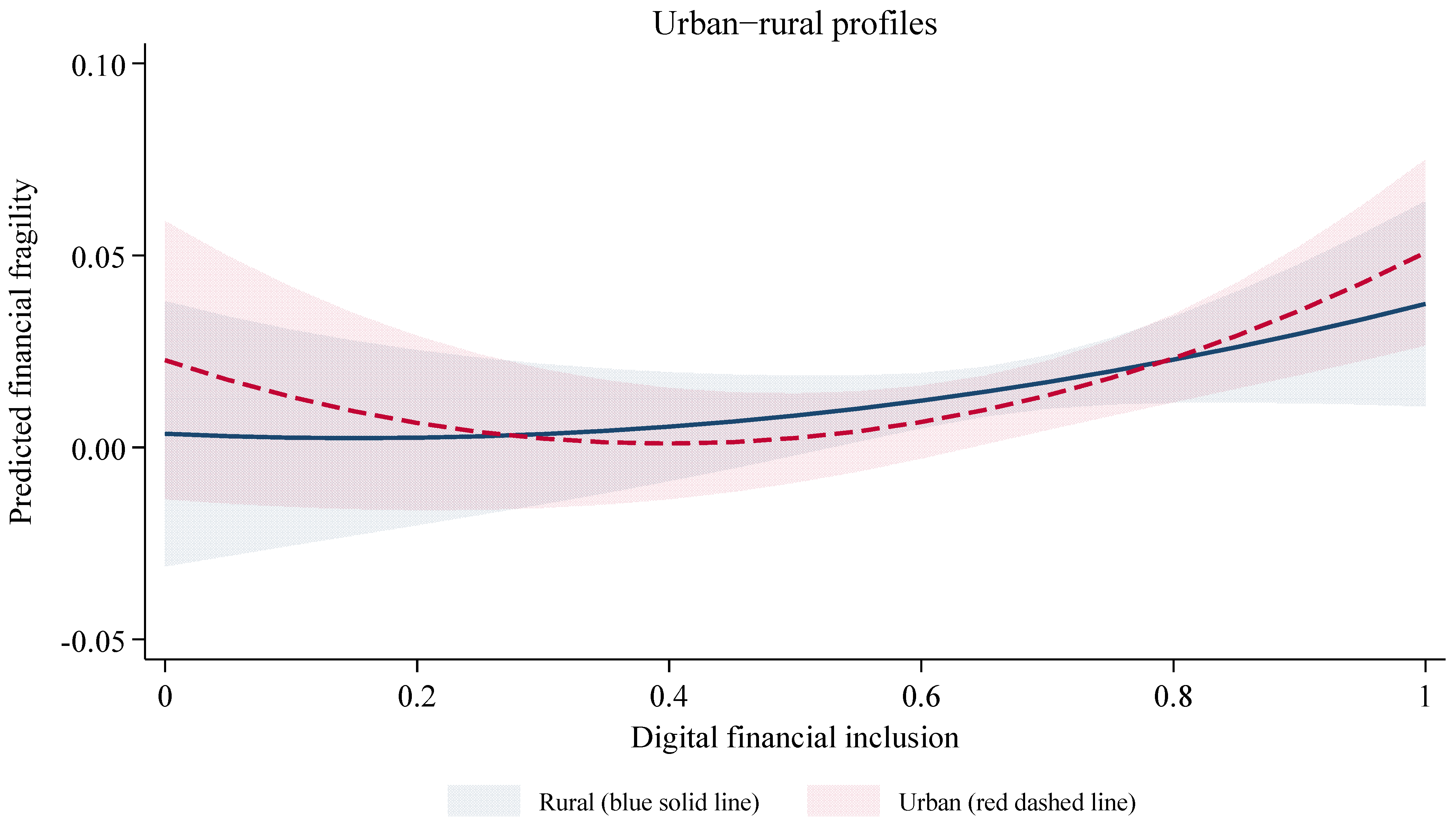
The results support a conservative interpretation. Evidence for broad urban–rural separation over the full DFI support is limited, but upper-tail diagnostics are more informative. The curvature and high-DFI slope tests indicate that the upward branch of the DFI–fragility curve is steeper for urban households. The high-DFI accumulation contrast, measured between the 75th and 90th percentiles of DFI, shows that the fitted increase in fragility over this range is larger for urban households than for rural households.
Figure 5 plots the predictive margins from the fully interacted specification. The figure displays the fitted profiles but does not replace the formal tests in Table 9. The urban curve bends upward more clearly in the upper part of the DFI distribution, whereas the rural curve is flatter and estimated with wider uncertainty. The visual pattern, therefore, matches the table: heterogeneity is localized on the risk-accumulation side of the curve, not across the full support.
This finding refines the main result. The average U-shaped relationship remains the central empirical finding. Urban–rural heterogeneity helps locate where the risk side of the relationship is more likely to emerge. For rural households, the evidence points more to uneven access and limited financial capability than to immediate overexposure. For urban households, where digital financial products are more widely used, risk governance should place greater weight on debt-service capacity, product transparency, and early warnings for repeated short-term borrowing.

6. Conclusions and Policy Implications

This study develops a theoretical framework with dual uncertainties and endogenous credit constraints and uses CFPS data to examine how DFI is associated with household financial fragility. The conclusions below are framed cautiously: the results identify a robust nonlinear pattern and channel-consistency evidence, while the exact turning point and causal interpretation remain subject to measurement and identification limitations.

6.1. Core Research Findings

This study arrives at the following three main findings.
This study documents a U-shaped relationship between digital financial inclusion and household financial fragility. The model predicts that at early stages of DFI development, improved information and lower transaction costs may support household financial resilience. Once DFI development passes a threshold, greater credit availability and risk-taking exposure may become more important: DFI is associated with higher household leverage, which in turn is associated with higher financial fragility. This nonlinear pattern remains visible across several robustness checks and offers a micro-level explanation for how digital finance can simultaneously support inclusion and contribute to household balance-sheet risk.
The impact of digital finance is heterogeneous. The main heterogeneity evidence is concentrated in the urban–rural exposure margin. The upper branch of the DFI–fragility curve is steeper for urban households, consistent with deeper exposure to digital credit, online wealth-management products, and platform-based financial services. Supplementary splits by macro DFI environment and traditional-finance density are retained as transparency checks, but do not provide strong evidence of full profile differences.
Mechanism tests indicate that the leverage channel is the more robust transmission margin. The risk asset allocation channel shows a nonlinear pattern and becomes more visible at higher DFI levels, but the evidence is weaker because risk assets are only an indirect proxy for perceived risk. The findings therefore support a balanced interpretation: DFI may improve inclusion, but mature digital-finance environments require stronger household risk governance.

6.2. Contributions

The findings of this study contribute to the theoretical development of household finance and digital finance in three ways.
In the first place, we endogenize both the information effect and the constraint effect within a unified analytical framework, thereby supplying the micro-foundations of its “double-edged sword” nature. Unlike previous studies that have either emphasized the inclusive value (Tao et al. 2023; Wu and Wu 2023) or warned of the risks (Hu et al. 2024; Chen and Liu 2024), our research is among the first to theoretically model and empirically validate the trade-off between these two opposing forces. By constructing a unified intertemporal decision model, this paper reveals how the two effects trade off as digital finance deepens, providing a more complete theoretical picture for understanding the complex impacts of financial innovation at the county level.
Next, we advance the field toward a nonlinear perspective. Through theoretical derivation and multi-method empirical tests, we confirm a robust U-shaped relationship between digital finance and household financial fragility. This finding implies that evaluations of digital finance should be conditioned on the development stage, supplanting the simple beneficial-or-harmful dichotomy with a threshold logic.
Ultimately, methodologically, our forward-looking financial vulnerability indicator translates the probability of financial distress from the theoretical model into an operational empirical variable via Monte Carlo simulation. This approach overcomes the limitations of traditional static indicators (such as debt-to-income ratios or delinquency status) by providing an ex ante measure of vulnerability that captures the probability of distress under income shocks. This methodological innovation achieves an effective linkage between theoretical constructs and empirical measurement, and provides a more precise measurement tool for subsequent research on household financial fragility.

6.3. Policy Implications

Based on the conclusions, we propose the following targeted policy recommendations:
Regulation should be dynamic and forward-looking, and it can be anchored to the estimated threshold. We recommend a monitoring system that tracks county-level digital-finance development against household leverage and triggers enhanced prudential review once a county crosses into the risk-accumulation region identified here—operationally, when the local index approaches the estimated inflection band and the share of households in the medium-or-higher fragility grades begins to rise. Concretely, regulators could (i) impose graduated, income-linked caps on digital consumer-credit lines that tighten as a borrower’s debt-service-to-income ratio approaches the 30% threshold used in our fragility measure; (ii) require platforms operating in high-penetration counties to run forward-looking repayment-capacity stress tests under standardized income-shock scenarios, mirroring the simulation logic of our indicator; and (iii) differentiate supervisory intensity by product, applying light-touch oversight to payments and savings while subjecting digital credit and complex investment products to stricter suitability and disclosure requirements. Tying the trigger to an observable, regularly updated threshold makes the regime rule-based rather than discretionary and gives platforms advance notice of when tighter standards apply.
Policy should address the distributional impacts of digital finance and prioritize protection for vulnerable groups. For people with low financial literacy, rural residents, and low-income households, financial education should move beyond general knowledge dissemination to teaching actionable decision-making skills, with particular emphasis on debt management, rollover costs, and contract interpretation. In the longer term, policymakers should consider a personal debt-resolution mechanism suited to China’s institutional context to provide legal relief for households in substantive debt distress and to prevent individual risks from propagating to the wider society.
Policy should promote functional complementarity and coordinated governance between traditional and digital finance. Incumbent financial institutions have risk-management experience, while digital platforms have broad reach and data-processing capacity. Policy should encourage transparent, inclusive products that combine these strengths, while ensuring that household leverage generated through digital channels is incorporated into macro-financial stability assessments.

6.4. Research Limitations and Future Outlook

Identification strategy: The identification strategy reduces but does not eliminate endogeneity concerns. The shift-share IV uses predetermined telecommunication infrastructure and terrain-related deployment costs interacted with aggregate internet diffusion. County and year fixed effects, region-specific trends, and over-identification tests mitigate obvious confounding channels, but they cannot prove the exclusion restriction. Historical infrastructure may still be correlated with unobserved time-varying local development, institutional quality, financial culture, or policy implementation. The IV estimates should therefore be read as supportive causal evidence rather than definitive proof. Future research could exploit digital-finance regulation, platform-entry restrictions, or staggered policy pilots as quasi-natural experiments.
Theoretical model: The theoretical model is deliberately parsimonious. It formalizes the sufficient conditions under which DFI can generate a U-shaped fragility profile, but it is not a fully estimated structural household portfolio model. Parameters such as the attention distortion, signal processing capacity, and the exact cognitive threshold are not directly observed. The model should therefore be interpreted as a disciplined mechanism framework that motivates the empirical specification, not as a complete representation of household decision-making.
Measurement of the fragility indicator: The forward-looking fragility indicator is calibrated rather than estimated from realized default data. Its level depends on the assumed shock distribution, debt-service benchmark, liquidity ratio, basic-expenditure ratio, sensitivity weights, and distress threshold. We report the full formula and threshold sensitivity to make the measure reproducible, but the high concurrent AUC is a validation against a related contemporaneous benchmark, not proof of long-run predictive accuracy. Future CFPS waves or lender-side default records are needed to test true out-of-sample predictive validity.
Measurement of mechanisms and DFI exposure: The mechanism variables are imperfect proxies. Risk asset captures revealed risky-asset allocation but cannot distinguish rational diversification from overconfidence, product complexity, or algorithmically induced risk misperception. Debt assets reflect both supply-side credit access and household demand for borrowing. Direct measures of subjective beliefs, financial literacy, platform recommendations, loan pricing, rollover behavior, and lender-side credit supply would allow a sharper test of the information and credit-constraint channels.
External validity: External validity should be treated cautiously. China’s rapid digital-finance expansion provides useful variation, but the location of the turning point is likely to depend on regulatory intensity, consumer-protection rules, credit-bureau coverage, and baseline financial literacy. Cross-country evidence and institution-specific comparisons would be valuable for determining whether the same nonlinear mechanism appears in other financial systems.

Supplementary Materials

The following supporting information can be downloaded at: https://www.mdpi.com/article/10.3390/risks14070164/s1.

Author Contributions

Conceptualization, W.Z. and X.T.; methodology, W.Z.; formal analysis, W.Z.; data curation, W.Z.; writing—original draft preparation, W.Z.; writing—review and editing, W.Z. and X.T.; supervision, X.T. All authors have read and agreed to the published version of the manuscript.

Funding

This research received no external funding.

Institutional Review Board Statement

The CFPS program is ethically reviewed and approved by the Biomedical Ethics Committee of Peking University. This study uses anonymized secondary survey data and does not involve new data collection from human participants.

Data Availability Statement

The original contributions presented in this study are included in the Supplementary Materials. Further inquiries can be directed to the corresponding author.

Conflicts of Interest

The authors declare no conflicts of interest.

Appendix A. Additional Heterogeneity Diagnostics

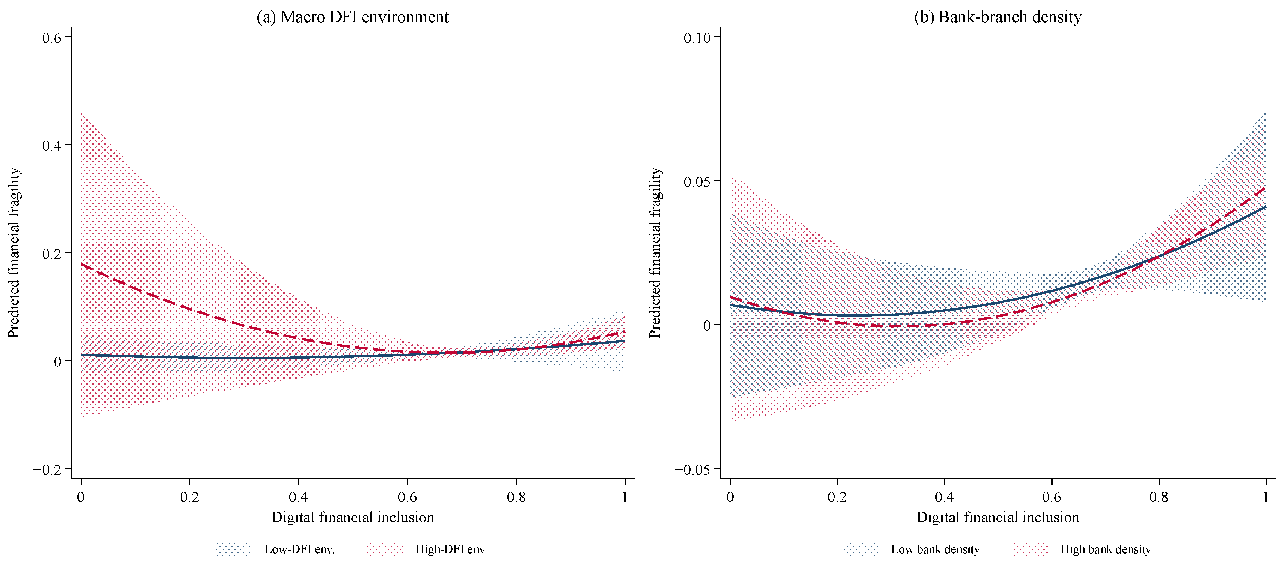
Figure A1 reports the regional macro DFI environment and traditional-finance splits. These tests are retained for transparency but are not treated as the main results. The macro DFI split is descriptive because it is constructed from the DFI distribution itself. The traditional-finance split is based on median bank-branch density. Neither dimension provides strong evidence that the full quadratic DFI–fragility profile differs across groups. Table A1, therefore, reports the difference tests explicitly. The weak p-values support the main-text decision to focus on urban–rural exposure rather than to overstate regional heterogeneity.
Figure A1. Additional heterogeneity diagnostics: macro DFI environment and traditional finance. Notes: Each panel plots predicted household financial fragility on the vertical axis against digital financial inclusion (DF) on the horizontal axis, separately for two groups. Panels show point (estimates lines) with 95% confidence intervals (shaded areas). In panel (a), groups are based on high vs low macro DFI environment. In panel (b), groups are based on high vs. low bank-branch density.
Risks 14 00164 g0a1
Table A1. Shape diagnostics for supplementary heterogeneity dimensions. The table reports p-values from fully interacted quadratic models. These dimensions are retained as transparency checks and are not emphasized as main heterogeneity findings.
DimensionFull ProfileCurvatureSlope p75Slope p90
Macro DFI environment0.4060.1880.8720.328
Traditional finance0.6220.4100.3320.338
Notes: The macro DFI split is based on the county–year mean DFI distribution. The traditional-finance split is based on median bank-branch density.

References

  1. Akerlof, Karen L., Paul L. Delamater, Caroline R. Boules, Crystal R. Upperman, and Clifford S. Mitchell. 2015. Vulnerable Populations Perceive Their Health as at Risk from Climate Change. International Journal of Environmental Research and Public Health 12: 15419–33. [Google Scholar] [CrossRef] [Scilit] [PubMed]
  2. Ampudia, Miguel, Has van Vlokhoven, and Dawid Żochowski. 2016. Financial fragility of euro area households. Journal of Financial Stability 27: 250–62. [Google Scholar] [CrossRef] [Scilit]
  3. Bank for International Settlements. n.d. Credit to the Non-Financial Sector [Data Set]. BIS Data Portal. Available online: https://data.bis.org/topics/TOTAL_CREDIT/data (accessed on 10 December 2025).
  4. Borusyak, Kirill, Peter Hull, and Xavier Jaravel. 2022. Quasi-experimental shift-share research designs. The Review of Economic Studies 89: 181–213. [Google Scholar] [CrossRef] [Scilit] [PubMed]
  5. Campbell, John Y. 2006. Household finance. The Journal of Finance 61: 1553–604. [Google Scholar] [CrossRef] [Scilit]
  6. Chen, Fuzhong, and Xin Liu. 2024. How does Internet Financial Product Participation Matter for Household Financial Vulnerability? Evidence from China. Journal of Family and Economic Issues. [Google Scholar] [CrossRef] [Scilit]
  7. Chen, Yiru, Li Liu, and Sufang Zheng. 2025. Impact of digital financial inclusion on rural revitalization. Finance Research Letters 85: 108071. [Google Scholar] [CrossRef] [Scilit]
  8. Chernozhukov, Victor, Denis Chetverikov, Mert Demirer, Esther Duflo, Christian Hansen, Whitney Newey, and James Robins. 2018. Double/debiased machine learning for treatment and structural parameters. The Econometrics Journal 21: C1–C68. [Google Scholar] [CrossRef] [Scilit]
  9. Diamond, Douglas W., and Anil K. Kashyap. 2016. Liquidity requirements, liquidity choice, and financial stability. In Handbook of Macroeconomics. Edited by John B. Taylor and Harald Uhlig. Amsterdam: Elsevier, vol. 2, pp. 2263–303. [Google Scholar] [CrossRef] [Scilit]
  10. Fagereng, Andreas, Helene Onshuus, and Kjersti N. Torstensen. 2024. The consumption expenditure response to unemployment: Evidence from Norwegian households. Journal of Monetary Economics 146: 103578. [Google Scholar] [CrossRef] [Scilit]
  11. Fort, Margherita, Francesco Manaresi, and Serena Trucchi. 2016. Adult financial literacy and households’ financial assets: The role of bank information policies. Economic Policy 31: 743–82. [Google Scholar] [CrossRef] [Scilit]
  12. Fu, Lingyan. 2024. Digital Financial Inclusion and Financial Vulnerability Analysis of the Household Economy—Empirical Evidence Based on CFPS. Applied Mathematics and Nonlinear Sciences 9. [Google Scholar] [CrossRef] [Scilit]
  13. Goldsmith-Pinkham, Paul, Isaac Sorkin, and Henry Swift. 2020. Bartik Instruments: What, When, Why, and How. American Economic Review 110: 2586–624. [Google Scholar] [CrossRef] [Scilit]
  14. Guo, Feng, Jingyi Wang, Fang Wang, Tao Kong, Xun Zhang, and Zhiyun Cheng. 2020. Measuring China’s Digital Financial Inclusion: Index Compilation and Spatial Characteristics. China Economic Quarterly 19: 1401–18. [Google Scholar] [CrossRef]
  15. He, Rong, Heqing Li, Zeng Lian, and Jie Zheng. 2020. The effect of culture on consumption: A behavioral approach. Journal of Asian Economics 67: 101180. [Google Scholar] [CrossRef] [Scilit]
  16. Hu, Debao, Fang Guo, Jianing Shang, and Xinyue Zhang. 2024. Does digital finance increase household Risk-taking? Evidence from China. International Review of Economics & Finance 93: 1197–210. [Google Scholar] [CrossRef] [Scilit]
  17. Kimball, Miles S. 1990. Precautionary Saving in the Small and in the Large. Econometrica 58: 53–73. [Google Scholar] [CrossRef] [Scilit]
  18. Korteling, Johan E. (Hans), Geerte L. Paradies, and Josephine P. Sassen-van Meer. 2023. Cognitive bias and how to improve sustainable decision making. Frontiers in Psychology 14: 1129835. [Google Scholar] [CrossRef] [Scilit] [PubMed]
  19. Lai, Lucy, and Samuel J. Gershman. 2024. Human decision making balances reward maximization and policy compression. PLoS Computational Biology 20: e1012057. [Google Scholar] [CrossRef] [Scilit] [PubMed]
  20. Lei, Wenjing, Siqi Hu, and Carol Hsu. 2023. Unveiling the process of phishing precautions taking: The moderating role of optimism bias. Computers & Security 129: 103249. [Google Scholar] [CrossRef] [Scilit]
  21. Leland, Hayne E. 1968. Saving and Uncertainty: The Precautionary Demand for Saving. The Quarterly Journal of Economics 82: 465. [Google Scholar] [CrossRef] [Scilit]
  22. Liu, Jianhe, Yuan Chen, Xuanyu Chen, and Bin Chen. 2024. Digital financial inclusion and household financial vulnerability: An empirical analysis of rural and urban disparities in China. Heliyon 10: e35540. [Google Scholar] [CrossRef] [Scilit] [PubMed]
  23. Liu, Menghao, and Yangbin Zhang. 2024. Study on the Impact of Digital Finance on Risky Financial Asset Allocation of Chinese Households. Journal of Statistics and Economics 1: 1–6. [Google Scholar] [CrossRef] [Scilit]
  24. Lusardi, Annamaria, and Olivia S. Mitchell. 2014. The economic importance of financial literacy: Theory and evidence. Journal of Economic Literature 52: 5–44. [Google Scholar] [CrossRef] [Scilit] [PubMed]
  25. Michelangeli, Valentina, and Cristiana Rampazzi. 2016. Indicators of Financial Vulnerability: A Household Level Study. SSRN Electronic Journal. [Google Scholar] [CrossRef] [Scilit]
  26. Modigliani, Franco, and Richard H. Brumberg. 1954. Utility Analysis and the Consumption Function: An Interpretation of Cross-Section Data. Edited by Kenneth K. Kurihara. Post-Keynesian Economics. New Brunswick: Rutgers University Press, pp. 388–436. [Google Scholar]
  27. Peng, Geng, and Fang Liu. 2024. Digital inclusive finance and the resilience of households involved in financial markets. Finance Research Letters 69: 106288. [Google Scholar] [CrossRef] [Scilit]
  28. Qian, Yanhong, Lei Yan, and Wenli Huang. 2025. How does digital inclusive finance affect household financial vulnerability? Emerging Markets Finance and Trade 61: 1293–314. [Google Scholar] [CrossRef] [Scilit]
  29. Simonse, Olaf, Wilco W. Van Dijk, Lotte F. Van Dillen, and Eric Van Dijk. 2024. Economic predictors of the subjective experience of financial stress. Journal of Behavioral and Experimental Finance 42: 100933. [Google Scholar] [CrossRef] [Scilit]
  30. Song, Sang-yoon. 2019. Leverage, Hand-to-Mouth Households, and Heterogeneity of the Marginal Propensity to Consume: Evidence from South Korea. Review of Economics of the Household 18: 1213–44. [Google Scholar] [CrossRef] [Scilit]
  31. Tao, Zhe, Xican Wang, Jing Li, and Xiaobei Wei. 2023. How can digital financial inclusion reduces relative poverty? An empirical analysis based on China household finance survey. Finance Research Letters 58: 104570. [Google Scholar] [CrossRef] [Scilit]
  32. Tian, Geng. 2022. Influence of Digital Finance on Household Leverage Ratio from the Perspective of Consumption Effect and Income Effect. Sustainability 14: 16271. [Google Scholar] [CrossRef] [Scilit]
  33. Wang, Haijing, and Chao Meng. 2025. Digital finance and rural household consumption. Finance Research Letters 86: 108925. [Google Scholar] [CrossRef] [Scilit]
  34. Wang, Xingqi, and Zhenhua Mao. 2023. Research on the Impact of Digital Inclusive Finance on the Financial Vulnerability of Aging Families. Risks 11: 209. [Google Scholar] [CrossRef] [Scilit]
  35. Wu, Jinshun, and Luyao Wu. 2023. Impacts of digital inclusive finance on household entrepreneurship. Finance Research Letters 56: 104114. [Google Scholar] [CrossRef] [Scilit]
  36. Xie, Yu, and Jingwei Hu. 2014. An introduction to the China Family Panel Studies (CFPS). Chinese Sociological Review 47: 3–29. [Google Scholar] [CrossRef]
  37. Yang, Shiyu, Ye Qiu, Wanhuan Cai, and Dawei Wang. 2025. Digital financial inclusion, environmental governance and household economic resilience. Finance Research Letters 85: 108214. [Google Scholar] [CrossRef] [Scilit]
  38. Zhang, Dongyang, and Rui Guo. 2020. The consumption response to household leverage in China: The role of investment at household level. International Review of Financial Analysis 71: 101580. [Google Scholar] [CrossRef] [Scilit]
  39. Zhang, Ke, and Jing Pang. 2025. Does digital finance promote entrepreneurship? Evidence from city-level and household-level data in China. Applied Economics Letters 32: 637–43. [Google Scholar] [CrossRef] [Scilit]
  40. Zhang, Xinyi, and Yizhou Zhang. 2026. The impact of digital finance on household financial vulnerability: Evidence from China. Finance Research Letters 91: 109512. [Google Scholar] [CrossRef] [Scilit]
  41. Zhang, Yaning, Yanzhe Yuan, and Guobin Zhao. 2025. An empirical study on the impact of household debt level on consumption behavior: Based on the mechanism of the housing provident fund system and risk preference. Finance Research Letters 72: 106507. [Google Scholar] [CrossRef] [Scilit]
  42. Zhou, Wenwu, and Xiabiao Tian. 2026. Preventing poverty recurrence in rural China: Risk shocks, household behavior, and sustainable livelihood strategies. Sustainable Development 34: 608–36. [Google Scholar] [CrossRef] [Scilit]
Figure 1. Trends in China’s DFI (2014–2022).
Risks 14 00164 g001
Figure 2. Area under the curve. Note: The receiver operating characteristic (ROC) curve evaluates the concurrent validity of the simulated forward-looking fragility indicator against the actual financial distress dummy.
Risks 14 00164 g002
Figure 3. Correlation matrix of key variables. Notes: The color gradient from blue to red represents Pearson correlation coefficients ranging from −1 to 1. Significance levels are denoted by asterisks: *** p < 0.01, * p < 0.1.
Risks 14 00164 g003
Figure 4. Kernel density plot with tipping point. Notes: The estimated U-shaped turning point is 0.273 in the baseline fixed-effects specification. The left side is interpreted as the inclusive-optimization region, and the right side as the risk-accumulation region. The threshold is an empirical warning band rather than a deterministic policy cutoff.
Risks 14 00164 g004
Figure 5. Predictive margins by urban–rural status. Notes: The figure plots predicted household financial fragility on the vertical axis against digital financial inclusion (DF) on the horizontal axis. The solid blue line shows the predicted profile for rural households, and the dashed red line shows the predicted profile for urban households. Shaded areas indicate 95% confidence intervals.
Risks 14 00164 g005
Table 1. Household risk-grade distribution based on the forward-looking indicator.
Risk GradeProbability IntervalNumber of HouseholdsProportion (%)Theoretical Interpretation
Extremely Low=020,96287.39Financially robust, strong ability to withstand shocks
Low(0, 0.1]22999.58Slight risk exists, but overall controllable
Medium(0.1, 0.3]3841.60Faces some pressure, requires attention
High(0.3, 0.6]560.23Financially fragile, easily affected by shocks
Very High>0.62851.19Highly financially fragile, very vulnerable to shocks
Note: Risk grades are determined by the simulated probability of financial distress over 1000 Monte Carlo iterations for each household under standard income shocks.
Table 2. Predictive performance under different thresholds.
ThresholdSensitivityPrecisionAccuracy
0.2 1.0000.6680.995
0.251.0000.7050.997
0.31.0000.7570.997
0.351.0000.7770.997
0.41.0000.8060.997
Notes: The table reports classification metrics of the forward-looking fragility indicator against the contemporaneous financial distress dummy across alternative thresholds. The metrics are used for concurrent validation, not as evidence of realized future default.
Table 3. Descriptive statistics of main variables.
MeaningMeanSDMinMaxN
Dependent Variable
FragilityFinancial fragility0.0160.1060.0001.00023,986
Core Independent Variable
DFIDigital financial inclusion index0.6320.2090.0001.00023,986
Control Variables
ageAge (squared/100)28.46414.7353.24090.25023,986
genderGender (male = 1)0.5240.4990.0001.00023,986
eduYears of education7.6974.7100.00022.00023,986
marryMarital status (married = 1)0.8550.3520.0001.00023,986
healthHealth status (1–5)3.1161.2111.0005.00023,986
urbHukou (urban = 1)0.4790.5000.0001.00023,986
Household and Economic Variables
houseownHomeownership (yes = 1)0.8750.3300.0001.00023,986
incomepLog household per capita income2.1552.4390.01514.50023,986
Note: The sample consists of 23,986 household-year observations from the China Family Panel Studies (CFPS) for the years 2014–2022.
Table 4. Baseline regression results.
Variable(1) Linear(2) Linear + FE(3) Quadratic(4) Quadratic + FE
Fragility
DFI 0.0040.004−0.033−0.052 *
(0.021)(0.021)(0.029)(0.030)
DFI 2 0.064 **0.095 ***
(0.029)(0.030)
age −0.000 ** −0.000 **
(0.000) (0.000)
edu 0.000 0.000
(0.000) (0.000)
marry −0.001 −0.001
(0.005) (0.005)
health 0.001 * 0.001 *
(0.001) (0.001)
urb −0.000 −0.001
(0.006) (0.006)
houseown −0.004 −0.004
(0.003) (0.003)
incomep −0.005 *** −0.005 ***
(0.001) (0.001)
Constant0.011 *0.024 **0.014 **0.030 ***
(0.006)(0.010)(0.007)(0.010)
N21,95321,79021,95321,790
R20.4090.4140.4090.415
Notes: The dependent variable is the forward-looking financial fragility indicator. All models include county and year fixed effects. Standard errors are in parentheses. *** p < 0.01, ** p < 0.05, * p < 0.1.
Table 5. Robustness of the nonlinear DFI–financial fragility relationship.
(1)(2)(3)(4)(5)(6)
VariableFragilityFinsmFragilityFragilityFragilityFragility
DFI −0.048 *−0.267 ** −0.017−0.046−0.102 ***
(0.026)(0.111) (0.030)(0.030)(0.036)
DFI 2 0.085 ***0.349 *** 0.064 ***0.096 ***0.063 **
(0.026)(0.109) (0.022)(0.032)(0.027)
L1_DFI −0.060 *
(0.036)
L1_ DFI 2 0.095 ***
(0.033)
Turning point0.2830.3820.3150.1370.2390.800
Year FEYESYESYESYESYESYES
Household FEYESYESYES---
ControlsYESYESYESYESYESYES
Constant0.028 ***0.294 ***0.045 ***0.023 ***0.0370.000
(0.009)(0.040)(0.014)(0.008)(0.037)(0.001)
N21,79021,79013,17723,82021,79014,674
R20.4170.5380.0100.0200.4150.01
Notes: Standard errors are in parentheses. The table reports turning points computed as β 1 / 2 β 2 . *** p < 0.01, ** p < 0.05, * p < 0.1.
Table 6. Endogeneity tests.
Variable(1)(2)(3)(4)
OLS2SLSLIMLGMM
DFI −0.052 *−0.236 *−0.236 *−0.235 *
(0.029)(0.128)(0.128)(0.128)
DFI 2 0.096 ***0.225 ***0.225 ***0.227 ***
(0.030)(0.059)(0.059)(0.055)
ControlsYESYESYESYES
Year and County FEYESYESYESYES
Constant0.031 ***
(0.010)
N23,82021,79021,79021,790
Adj. R20.00750.00440.00440.0045
First-stage regression results
Variable DFI DFI 2
IVterrain,year−0.003 ***
(0.000)
−0.003 ***
(0.000)
iv1−0.000 ***
(0.000)
−0.000 *
(0.000)
iv20.002 ***
(0.000)
0.001 ***
(0.000)
F-statistic161.48 ***431.08 ***
SW F-statistic153.35***387.63 ***
Instrument validity tests
Kleibergen-Paap rk LM108.237p < 0.01Passed
Kleibergen-Paap Wald F99.190>13.43
(10% level)
Passed
Over-identification testp = 0.934 Passed
Endogeneity test (Hausman)0.183>0.05Not rejected
Notes: The endogenous regressors are DFI and its quadratic term. The instrument set is constructed by interacting 1984 county landline telephone density, aggregate internet penetration, and terrain ruggedness. All specifications include baseline controls, county fixed effects, and year fixed effects. Standard errors are in parentheses. *** p < 0.01, * p < 0.1.
Table 7. Mediation mechanism tests results: full-sample nonlinear model.
Variable(1)(2)
Risk AssetDebt Asset
DFI −0.076 ***0.013
(0.019)(0.034)
DFI 2 0.089 ***0.082 **
(0.021)(0.035)
ControlsYESYES
Year FEYESYES
Constant0.033 ***0.110 ***
(0.008)(0.019)
N17,35223,820
adj. R20.0130.010
Notes: Columns (1) and (2) report associations between DFI (linear and quadratic terms) and the mechanism proxies risk asset and debt asset, respectively. All models include baseline controls, county fixed effects, and year fixed effects. Standard errors are in parentheses. *** p < 0.01, ** p < 0.05.
Table 8. Subgroup mechanism test.
Test StepVariableBelow Turning Point
(DFI < 0.523)
Above Turning Point
(DFI ≥ 0.523)
Risk-taking
Step 1: DFI → risk assetDFI−0.0060.053 ***
(0.006)(0.012)
Step 2: risk asset → fragilityrisk asset−0.0100.026 *
(0.020)(0.014)
DFI−0.0050.027 **
(0.027)(0.011)
ControlsYESYES
N235215,000
Leverage
Step 1: DFI → debt assetDFI0.097 ***0.107 ***
(0.032)(0.023)
Step 2: debt asset → fragilitydebt asset0.171 ***0.102 ***
(0.052)(0.009)
DFI−0.0070.016 *
(0.022)(0.009)
ControlsYESYES
N435919,461
Notes: The sample is split using the IV-estimated turning point (DFI = 0.523). All subgroup regressions include baseline controls, county fixed effects, and year fixed effects. Standard errors are in parentheses. *** p < 0.01, ** p < 0.05, * p < 0.1.
Table 9. Shape-based heterogeneity in the DFI–fragility curve.
Panel A. Group-Specific U-Shaped ProfilesFull SampleRuralUrban
DFI−0.052−0.009−0.093
(0.039)(0.046)(0.066)
[−0.130, 0.026][−0.100, 0.082][−0.223, 0.037]
DFI 2 0.096 ***0.0260.144 **
(0.033)(0.041)(0.065)
[0.029, 0.162][−0.056, 0.107][0.015, 0.273]
Turning point [95% CI]0.2730.1760.323
[−0.011, 0.558][−1.402, 1.754][0.047, 0.599]
Endpoint slopes, min/max−0.052/0.139−0.009/0.040−0.093/0.195
U-shape test p0.0930.4220.080
N21,79011,3999918
County clusters967596
R 2 /within R 2 0.415/0.0070.428/0.0100.399/0.009
Controls and Household & year FEYesYesYes
Panel B. Urban–rural shape contrasts
TestStatistic/Estimate95% CIp-Value
Full profile equality2.345--0.101
Curvature equality4.090--0.046
Slope difference at p750.041[0.003, 0.080]0.034
Slope difference at p900.059[0.005, 0.113]0.033
High-DFI accumulation contrast0.005[0.000, 0.009]0.033
Turning-point difference, urban–rural0.246[−0.381, 0.873]0.439
Notes: Panel A reports group-specific quadratic profiles. The U-shape test is the intersection-union test based on a negative slope at the lower end of observed DFI support and a positive slope at the upper end. Panel B is estimated from the pooled fully interacted quadratic model. Full profile equality jointly tests the urban–rural differences in the linear and quadratic DFI terms. DFI support is min = 0.000, median = 0.680, p75 = 0.766, p90 = 0.864, max = 1.000. ** p < 0.05, *** p < 0.01.
Disclaimer/Publisher’s Note: The statements, opinions and data contained in all publications are solely those of the individual author(s) and contributor(s) and not of MDPI and/or the editor(s). MDPI and/or the editor(s) disclaim responsibility for any injury to people or property resulting from any ideas, methods, instructions or products referred to in the content.