

Article

The Kerper–Bowron Method: A Foundational Change for Service Contract Claim Estimation and Accounting
by
John Kerper
and
Lee Bowron
*
Kerper and Bowron, LLC, Birmingham, AL 35209, USA
*
Author to whom correspondence should be addressed.
Risks 2026, 14(3), 44; https://doi.org/10.3390/risks14030044
Submission received: 29 December 2025 / Revised: 29 January 2026 / Accepted: 10 February 2026 / Published: 24 February 2026
(This article belongs to the Special Issue Advances in Risk Models and Actuarial Science)

Abstract

The Kerper–Bowron Method (KB Method) is a patent-pending approach that revolutionizes service contract loss estimation and accounting by introducing a precise, contract-level approach to forecasting expected losses and cancellations. Building on a prior 2007 paper, this update presents the Earned Contract formula, aligning with Solvency II and modern accounting standards. By leveraging a probabilistic exposure base and Generalized Linear Models, the KB Method enhances accuracy in claims and cancel liabilities as well as other liability and asset estimates across global service contract markets. This methodology offers superior precision, automation, and compliance, redefining actuarial and financial practices for vehicle and other service contracts.

1. Introduction

Service contracts (also known as extended warranties) represent a significant segment of the global insurance and consumer protection market, with annual sales projected to reach approximately $250 billion by 2031 (Grandview Research 2025).
These contracts cover repair, maintenance, or accidental damage for consumer durables ranging from vehicles to appliances and electronics. Accurate loss estimation and revenue recognition are critical for various entities including insurers, administrators, and retailers. Accurate recognition is essential for both business performance and regulatory compliance.
Traditional actuarial practice for service contracts relies on aggregate earnings curves and block-level reserving methods, which date back over 40 years (Kerper and Bowron 2007; Diamantoukos 1991).
These approaches use industry averages or summary firm experience to estimate earned premiums and expected losses, often with subjective assumptions.
Recent regulatory frameworks have heightened the need for precision:
  • Solvency II (Directive 2009/138/EC) requires exact equivalence to the ideal equation for finite risks.
  • IFRS 17 requires a similar calculation of expected cash flows.
  • ASC 606 (U.S. GAAP) requires revenue recognition based on the industry that it applies. For service contracts, this is also equal to expected cash flows. Existing aggregate methods cannot satisfy these standards simultaneously while maintaining contract-level granularity, leading to inefficiencies in reserving, compliance, and capital management.
The Kerper–Bowron Method addresses these gaps by introducing a contract-level framework that generates precise, month-by-month probabilistic cash-flow projections using only point-of-sale data. The primary contribution is the first mathematical demonstration of exact equivalence to Solvency II’s ideal equation for finite, predictable risks, while achieving perfect alignment with IFRS 17 and ASC 606.
Scientific novelty: The method derives the Earned Contract formula, enabling contract-specific truth without reliance on aggregate approximations. This eliminates subjective overlays and provides auditable, forward-looking estimates.
Practical significance: For service-contract administrators, reinsurers, and financial institutions, the method would reduce manual reserving work, enable real-time equity visibility, and support compliance across jurisdictions. It applies to all service contracts (vehicles, appliances, electronics, commercial equipment).
Some of these concepts were introduced in a previous paper by the same authors, “An Exposure Based Approach to Automobile Warranty Ratemaking and Reserving”, which was originally published in Casualty Actuarial Society Forum, Winter 2007. Terminology has been updated to conform with current industry norms.
The remainder of the paper is structured as follows:
  • Section 2—Introduces the fundamental concept of the Earned Service Contract, which is the basis for balance sheet and income statement items across the global service contract space.
  • Section 3—Provides a history of the service contract market.
  • Section 4—Reviews US and global accounting and insurance regulatory standards.
  • Section 5—Describes the current actuarial and industry practices to support estimates for future liabilities and revenue recognition for service contracts.
  • Section 6—Describes the Kerper–Bowron Method.
    • Section 6.1—Exposure Development.
    • Section 6.2—Model Development.
    • Section 6.3—Calculation of Expected Claims and Cancels by Valuation Period.
    • Section 6.4—Applications and Exposure Adjustments for Non-VSC Service Contracts.
  • Section 7—The impact of the Kerper–Bowron Method across various accounting and insurance regulatory standards.
  • Section 8—Applications to customer lifetime value.
  • Section 9—Conclusions.
The techniques underlying the Kerper–Bowron Method (“KB Method”) are much more precise than existing techniques. The KB Method provides a contract-level stream of future expected claim and cancellation payments, which are relevant for both actuarial and accounting estimates.
The stream of expected losses and cancellations by service contract redefines accounting and actuarial analysis across the globe and is consistent with accounting and actuarial standards, regulations, and laws worldwide.

2. Earned Service Contract

The heart of the KB Method is the stream of expected cash flows for the entire length of the contract. These expected cash flows drive the entire balance sheet by providing contract level estimates of all relevant liabilities.
Consider the expected loss cash flows from a single service contract loss estimate.
a = f 1 + f 2 + f 3 + + f e ,
where:
  • a = Total loss forecast at sale of the contract,
  • f = Forecast for liability for each month after sale of the contract,
  • e = Months till expiration (typically term + 1)
This value can now be defined to form an Earned Contract, which is the sum of the percentage of revenue recognition in each month over the valuation period:
E C = f 1 a + f 2 a + f 3 a + + f e a ,
where E C = Total Earned Contract = 1.
Now consider where:
E C i = f i a .
The percentage of contract recognized at time v is defined by:
E C v = i = 1 V E C i ,
The unearned contract at time v is defined by:
U E C v = 1   i = 1 v E C i = i = v + 1 e E C i ,
E C = E C 1 + E C 2 + E C 3 + + E C e = 1.00 .
These initial allocations form the basis for a variety of balance sheet calculations across the entire valuation period of the contract. Further below, we discuss some examples of asset, liability, and income items using this formula.
The initial E C calculation for unearned premium, as well as other balance sheet items in the entity, would not be updated for actual experience or model changes under most scenarios.1

3. A Brief History of Service Contracts

Service contracts are agreements that effectively extend the warranty coverage beyond the standard manufacturer’s warranty. In addition, many service contracts provide benefits not included in the manufacturer’s warranty such as accidental damage and maintenance. If the underlying collateral is financed, the amount for this coverage is typically added to the loan and financed with the underlying collateral.
The concept of warranties, including extended warranties, can be traced back to early commercial practices where sellers provided assurances to buyers about the quality or performance of goods. These warranties would be governed by contract law.
While service contracts did not exist before the 20th century, implied warranties—unspoken guarantees that a product would function as intended—were common in trade practices globally, particularly in Europe and early industrial societies.
When Ford introduced the Model T in 1908, no formal warranty was included, but informal promises of quality were made by manufacturers like Henry Ford. Maxwell Motor Company (now Chrysler) (Auburn Hills, MI, USA), offered a legally binding 90-day warranty. Customers were required to bring broken components to the factory themselves (Brown 2025).
The modern concept of service contracts began to take shape in the late 1950s, particularly in the automotive industry in the United States. As vehicles became more complex and expensive, manufacturers started offering factory warranties to assure buyers of reliability. In 1961, Lincoln Continental (Dearborn, MI, USA) offered the first 12 months/12,000 mile warranty and the idea quickly spread, and coverage expanded.
By the 1970s, the increasing complexity of vehicle components led manufacturers to reduce the duration and comprehensiveness of factory warranties, creating a gap that third-party providers filled with vehicle service contracts (Brown 2025). This period marked the rise of service contracts as a distinct product. Initially, manufacturers, dealers, or independent companies offered these contracts to cover repairs or replacements beyond the standard warranty period, typically for automobiles and electronics.
The growth of consumer electronics in the mid-20th century, such as televisions and appliances, further fueled demand for extended warranties as consumers sought protection against costly repairs (Bertolini 2007).
The 1970s saw significant growth in the extended warranty market, particularly in North America and Europe. In the United States, the Magnuson-Moss Warranty Act of 1975 was a pivotal regulatory development. This federal law clarified that service contracts were distinct from warranties because they were sold separately for a fee, unlike standard warranties included in the product price (Warranty Conference 2005). This distinction led to lighter regulation of service contracts compared to traditional warranties, allowing third-party providers to enter the market more easily.
In 1995, the National Association of Insurance Commissioners (NAIC) adopted Model #685, the Service Contracts Model Act. This provided states a template to regulate service contracts without classifying them as insurance, addressing consumer protection concerns like solvency, disclosures, and unfair practices while avoiding heavy insurance-style burdens (Pope et al. 2022).
Globally, the service contract market expanded as consumer goods became more prevalent across the developed world. The advent of home computing, the internet, and smartphones in the late 20th and early 21st centuries revolutionized the service contract industry. Providers began offering online platforms and mobile apps for customers to manage plans and file claims, increasing accessibility and convenience (Brown 2025).
Today, service contracts cover a wide range of products. Major categories include private passenger vehicles, recreational vehicles, electronics (including a large market in phones), appliances, and home service contracts which cover multiple systems. For electronics, accidental damage coverage will typically have substantially more claims than product failure.
Service contracts are placed on collateral ranging from USB drives to heavy equipment used by industry, with virtually everything in between.
Key developments include:
  • Diversification of Coverage: Initially focused on mechanical failures, modern service contracts may cover accidental damage and maintenance services. For example, auto service contracts might include towing or rental car reimbursement (Federal Trade Commission 2023).
  • Third-Party Administration: The rise of third-party administrators has introduced greater complexity and flexibility. These entities often act as obligors and create a layered ecosystem involving manufacturers, retailers, administrators, and insurers (Breitenstein 2020).
  • Customization and Innovation: Providers now offer tiered coverage plans tailored to consumer needs, such as high-mileage vehicle plans or coverage for luxury cars. Data-driven pricing strategies and predictive analytics have enabled providers to assess risks more accurately and offer competitive products (Brown 2025).

4. US and Global Standards for Accounting for Service Contracts

Accounting for extended warranties has been shaped by evolving standards, particularly in the US and globally through frameworks like ASC 606 and IFRS 17 (FASB 2014; ISAB 2017). Below is an overview of key accounting principles and their development:
Prior to 2018 in the United States, FASB Technical Bulletin 90-1 (1990) mandated that revenue from separately priced extended warranties be deferred and recognized on a straight-line basis over the contract term (Financial Accounting Standards Board 1990). This treated extended warranties as insurance policies, with revenue recorded as a liability (deferred revenue) under a pro-rata basis (Extended Warranty Profits 2004; Jiang and Dayley 2020).
The introduction of ASC 606 (U.S.) which was fully adopted in 2019 and IFRS 17 (global) in 2023 standardized revenue recognition for service contracts.
ASC 606 and IFRS 17 requires companies to allocate transaction prices to distinct performance obligations, ensuring that revenue is not recognized prematurely. This has increased accounting complexity, as companies must estimate standalone selling prices and track costs separately (Bashina 2025).
The steps are based on a five-step model: identifying the contract, performance obligations, transaction price, allocation, and recognition when obligations are satisfied. For service contracts, allocation and recognition are typically based on earnings curves as further discussed below.
In terms of service contracts, the obligation is to perform the terms of the underlying contract, which requires claims and potentially cancellation payments based on the underlying contract. The selling price is stable and recognized at the beginning of the contract, gross of cancellation provisions.
Further discussions of these standards in relation to the KB method are discussed below.

5. Current Actuarial Practices with Service Contracts

5.1. US Statutory Accounting—SSAP 65

SSAP 65 (Statement of Statutory Accounting Principles No. 65) governs statutory accounting in the United States for long duration contracts, which includes most service contracts.
SSAP 65, issued by the NAIC, provides guidance on accounting for property and casualty insurance contracts under US statutory accounting principles for estimating unearned premium reserves for long-duration contracts which have coverage periods of 13 months or longer and cannot be cancelled by the insurance company.
The unearned premium is subject to 3 tests under SSAP 65: Refund, Proportional, and Future Losses and Expenses. These are performed for the last 3 policy years plus the aggregate of the remaining older policy years. The required reserve is the maximum of the 3 tests for each of the policy year groups.
The reserve must be at this level or above. There is no requirement that the unearned premium not be redundant, which is different than the standards for loss reserves under NAIC instructions for loss reserve opinions.

5.1.1. Test 1: Refund Test

This liability is defined as the amount that would be returned to all customers upon cancellation of the service contract. For VSCs, refund rules under the contract are typically the lesser of the proportional amount of months and miles. For example, a customer purchases a new vehicle with a service contract of 84 months and 84,000 miles. After the first year (month 12), the customer requests a refund. The refund basis on time is 72/84 or 85.7% while the refund basis on mileage is (69,000/84,000) or 82.1%. The greater earnings are the mileage basis so a refund of 82.1% is made. There is no consideration of the underlying manufacturer’s warranty in the calculation.
This amount is typically lower than the proportional test below because of the lack of consideration of the underlying warranty as well as lower refunds for high mileage drivers. In addition, the requirement that a reserve must be held to fund all cancelled contracts is conservative since the consumer must initiate each cancellation.

5.1.2. Test 2: Proportional Test

This liability is defined as the calculated amount for the contracts to earn proportionally. Theoretically, this is the amount that would produce an equal expected loss ratio each month. The traditional formula is:
G r o s s   P r e m i u m × [ P r o j e c t e d   F u t u r e   L o s s e s   a n d   E x p e n s e s ÷ P r o j e c t e d   T o t a l   G r o s s   L o s s e s   a n d   E x p e n s e s ] .
In this case, the Gross Premium is the premium without consideration of cancellations.
Projected Future Losses are selected by the actuary using methodology appropriate to the data. Further discussion is below. Expenses include cancellations but in general most other expenses are paid before the underlying amounts are placed into an insurance company. However, some amounts such as the premium tax are paid at the beginning of the contract. Initial expenses will decrease the indicated proportional reserve, which is clear from the formula above.
This method can provide a good approximation, but issues can arise with the technique. Events that impact calendar years can distort the results. For example, an inflationary shock may impact the latter part of the contract, making proportionality difficult to maintain. Another issue is a low loss ratio program where minor fluctuations in losses can have major impacts on this test.

5.1.3. Test 3: Discounted Projected Future Losses and Expenses

The undiscounted amount is a variable in the Test 2 calculation above. As noted, the actuary has some discretion in how this amount is calculated and the ultimate selection. Discounting is at a risk-free rate.
For VSC programs with a credible volume of claims, it is customary for the actuary to separate the data into homogeneous groupings. Due to the wide variety of underlying manufacturers’ warranties and a large number of terms, this stratification is difficult to achieve. Typically, this grouping is done by the actuary by selecting various terms and initial mileage bands in an attempt to mimic the impact of the underlying warranty.
The data should include both losses and cancellations as each are liabilities of the fund. The data are triangulated by the purchase date of the contract and the loss date of the claim or the cancellation date. The age for the triangle is different than loss development, which measures the time between the occurrence of the loss and the date of the reserve change and/or payment transaction.
Age-to-age factors are calculated, and an ultimate liability is formed. Alternatively, the age can be calculated between the purchase date of the contract and the payment date of the loss. This technique would also include a measurement of IBNR in addition to the expected losses from the unearned premium reserve (Hayne 2007).
For newer cars at initial valuations, there is extreme immaturity until a significant percentage of the term has passed. Due to this, it is common for the actuary to select the Bornhuetter–Ferguson method for these contracts. Due to the sensitivity of the expected loss ratio to the overall results, this method is not accurate when underlying conditions of the book are changing.
The goal of this exercise is to project the indicated losses and cancellations from the unearned premium. As noted above, this liability is discounted at a risk-free rate. If Test 3 is the maximum test, the indicated unearned premium will effectively include a Premium Deficiency Reserve.

5.2. Earnings Curves

Accounting estimates are typically based on the concept of “Earning Curves”, which is a revenue recognition practice. Similar to the Earned Contract above, revenue is recognized on a predetermined basis based on earnings factors that range from 0.00 to 1.00 over the life of a contract.
A curve that has a linear basis from the beginning of the contract (0.00) to the end of the contract (1.00) is known as “pro-rata”. This is a very common basis for service contracts, especially used cars, which have no manufacturer’s warranty remaining, as well as collateral where the manufacturer’s warranty is immaterial, such as phones.
For vehicles that either have or are expected to have manufacturer’s warranty,2 it was initially common to use special formulaic curves such as the “Reverse-Rule-of-78s;”3 however, current best practice uses actuarial or statistical bases to determine these curves. The example below in Table 1 shows 3 potential curves for a 36 month contract.
In order to calculate the indicated earnings curve with sufficient data, the best practice would be to aggregate the losses (but not cancellations as was done for SSAP 65 analysis) by policy year or policy quarter and the age of the contract similar to above.
These amounts would be divided by the in-force contracts at each identical period, and the pure premium can be formed. This pure premium can be projected to the current period considering inflation and other factors. The selected pure premiums are allocated to form the earnings curve. These calculations are illustrated in Table 2 below.
From these values, monthly values can be interpolated, and an indicated earnings curve can be formed, as seen in Table 3 below.
In Table 3, columns (1) and (2) come from Table 2, column (3) is interpolated with weight, column (4) is each month’s value in (3) divided by the total of column (3), and column 5 is the cumulative sum of column (3) through each current month.
In the Kerper–Bowron method introduced below, earnings curves will be produced individually by contract based on the attributes of the specific contract.

5.3. European Service Contract Actuarial Practice

Actuaries in Europe use similar techniques as the ones presented above.
Monte–Carlo simulation in Europe is more common and is consistent with the reserve margins required for calculations. One technique used for this estimation is the Over-Dispersed Poisson (ODP) Model: The ODP model simulates claim counts and severities (European Parliament 2009).4
IFRS 17 and Solvency II require transparent documentation. Stochastic models provide auditable confidence intervals, while loss triangles are validated against historical benchmarks (European Parliament 2009).
In addition, there is usage of telematics from vehicles to predict vehicle repairs. Most effort in telematics appears to be centered around EV battery usage, which is an emerging technology issue (Winkler 2021).5

6. The Kerper–Bowron Method

The following sections introduce the KB Method. This method is fundamentally different from previous practices. The traditional methods project loss and cancellation by age from the sale of the contract. In the KB method, exposures are calculated that specifically exclude the time when the manufacturer’s warranty is in effect or the service contract has expired due to exceeding the mileage limitations of the contract.
The Kerper–Bowron Method calculates the Future Loss and Cancel Estimate (FLC) and the Future Loss Estimate (FL). At contract inception, the FL estimate underlies the Earned Contract estimate. At later valuations, applications are in liability estimation.
The projections under this method are made for each contract, based on the specific characteristics of each contract that are predictive of loss. A flow chart of the process is included in Appendix A of this paper.
The first step is to select a time period to form the model. This will be a calendar period in the past, such as one, two, or more years. Statistical analysis and judgment are critical in the period selection. Complete years are preferable to avoid seasonality issues. Note that this calendar period will only include a portion of contracts. Contract age will increase with the term as only the latter period of the older contracts is considered.
There are 3 major steps in performing the Kerper–Bowron Method: exposure development, model development, and projection. A brief summary of the method is shown below with additional sections further developing these concepts.
1.
Exposure Development and Associated Losses
Exposures are calculated that explicitly consider the manufacturer’s warranty using the implied age of the vehicle and the terms of the manufacturer’s warranty. The age of the vehicle could be determined by the in-service date but accurate information on this is not typically available. However, the model year of the vehicle may provide a good approximation. Historical driving patterns would be used if available to form exposures considering both the manufacturer’s warranty and terms of the service contract.6 Public data, as noted below, are also available.
Associated losses are claims that occurred during the selected period. This should include an IBNR estimate in order to project accurate future losses. A monthly IBNR loss development analysis would be required to demonstrate Solvency II functional equivalency, as shown below.
2.
Model Development
The firm has used Generalized Linear Models (“GLMs”) for client work, but other models may be appropriate. Artificial Intelligence and other type models may ultimately show higher predictive power, but the GLM has the advantage of being explainable to auditors and is open source. The GLM model predicts pure premium by contact characteristics.
S t u d y   P u r e   P r e m i u m = A s s o c i a t e d   L o s s e s ÷ A s s o c i a t e d   E x p o s u r e s .
3.
Projected Future Losses and Cancels
Future exposures are developed similar to (1). These exposures are adjusted for future cancellations. These future exposures are multiplied by the GLM parameters to form an initial future loss. These losses are then adjusted for seasonality and inflation, and an estimate of future cancellations is added to form the Projected Future Losses and Cancels by month (FLC).

6.1. Exposure Development

6.1.1. Exposure Development Theory

Exposures in property casualty insurance are a fundamental concept (Diamantoukos 1991). They relate to the basis of pricing insurance and loss reserving, especially where there is limited data.
For most lines, the exposure base is obvious. For a private passenger, it is Earned Car Year, which is one car insured for one year. Similarly, for homeowners, the exposure base is Earned House Year. For other lines, the exposure is different. Table 4 below gives some examples selected for other lines of insurance:
Service contracts have traditionally been analyzed by policy year.7
The KB Method changes the traditional policy year exposure base to a probabilistic exposure base for each month of the contract rather than the expected miles driven under a service contract. This prior paper calculated the mileage driven under a service contract (Kerper and Bowron 2007).
This is a more difficult exposure base to calculate. A VSC is fundamentally designed to mimic a manufacturer’s warranty for a longer period.
For example, a manufacturer’s warranty is typically expressed in months and miles for “Bumper to Bumper” and “Powertrain” coverages. If the terms are different, the Powertrain warranty is always longer.
  • Bumper-to-Bumper Warranty: Covers most vehicle components (e.g., electrical, suspension, air conditioning, engine) except wear-and-tear items (e.g., brake pads, wipers, tires). Exclusions vary by manufacturer.
  • Powertrain Warranty: Covers engine, transmission, driveshaft, differentials, and related components. Some manufacturers (e.g., Hyundai, Kia (both South Korea)) limit powertrain coverage beyond the bumper-to-bumper coverage to the original owner. If the bumper-to-bumper warranty has expired, this will provide more limited coverage under the warranty and additional coverage under the service contract.
A summary of bumper-to-bumper and powertrain warranties is shown below in Table 5.
A typical service contract effectively extends the term of the manufacturer’s warranty under the terms of the VSC to the term of the service contract.
For example, a VSC with a term of 96 months/96,000 miles on a new GMC truck (with 0 miles) will cover Bumper-to-Bumper from month 36 or an odometer reading of 36,000 miles (whichever comes first) to the VSC term. Similarly, Powertrain coverage will be from month 60 or an odometer reading of 60,000 miles.
Coverage is effective from month 36 or month 60 to month 96. Alternatively, coverage is effective from odometer 36,000 or odometer 60,000 to odometer 96,000 miles after the initial mileage at the purchase (“Expiration Miles”). As with the manufacturers’ warranty, exceeding either month 96 or the Expiration Miles will expire the contract.8
In order to evaluate the “Miles Driven” under a VSC, estimation must be made of the miles driven under the manufacturer’s warranty as well as miles driven within the VSC time period but exceeding the mileage terms of the service contract.
In order to calculate this range, assumptions can be made on the driving patterns of the underlying book. This is typically easy to do based on the underlying data, which will show odometer readings at the time of a claim or cancellation. The date and mileage information from these readings can be combined with the effective date of the contract as well as the initial miles on the vehicle at the time of sale. From this data, mileage distributions can be formed.

6.1.2. Exposure Calculations Using Public Data

The Puget Sound Study is a publicly available database that provides individual driving patterns (National Laboratory of the Rockies 2004–2006).
The data are slightly below the national driving average—the average annual miles driven by American drivers in 2005 was approximately 13,657 miles per driver (Highway Statistics 2005). The purpose of the study was to determine the effectiveness of hypothetical tolls, which would incentivize decreases in average miles driven. However, this impact does not appear to be material and is a good proxy for driving habits.
In order to evaluate the exposures, a simple lognormal curve is fitted to the monthly miles per vehicle using the study data.
These calculations are shown in Table 6:
A histogram of fitted versus actual values shows good fit for the study data to the lognormal distributions, seen in Figure 1. There is a slight downward bias at the tail for this data.
The exposure, or percent of service contracts expected to be eligible for service contract benefits under the terms of the service contract and adjusting for the warranty, is defined as:
S e r v i c e   C o n t r a c t   E x p o s u r e = P r o b a b i l i t y   a   S e r v i c e   C o n t r a c t   H a s   N o t   E x p i r e d P r o b a b i l i t y   a   M a n u f a c t u r e r s   W a r r a n t y   H a s   N o t   E x p i r e d .
This can be calculated using the inverse lognormal function with the parameters above. An example is shown below in Table 7 for a hypothetical service contract.
The exposure can be more formally defined as:
  • M i = Month i,
  • A = Service contract’s term miles,
  • B = Service contract’s term months,
  • C = Manufacturer’s warranty term miles,
  • D = Manufacturer’s warranty term months,
  • E = Vehicle’s mileage at purchase of service contract,
  • μ = Mean of the natural logs of monthly mileage for all contracts, and
  • σ = Standard deviation of the natural logs of monthly mileage for all contracts.
The exposure under the terms of the service contract in month i is given by:
s c M i ; μ , σ = Φ l n ( A M i 0.5 )   μ σ ,   i f   M i B 0 ,   o t h e r w i s e .
Similarly, the exposure under the terms of the manufacturer’s warranty in month i is given by:
m w M i ; μ , σ = Φ l n ( C E M i 0.5 )   μ σ ,   i f   M i D 0 ,   o t h e r w i s e .
Notice how the vehicle’s mileage at the purchase of the service contract (E) is subtracted from the manufacturer’s warranty term miles (C). This is because the manufacturer’s warranty expires once the odometer of the vehicle reaches the term miles. This is not the case for the service contract, which instead adds the term miles (A) to the starting odometer and thus does not take the starting odometer into account in its exposure calculations.
The service contract’s total exposure at a given month is defined by:
s c M i m w ( M i ) .
Further, the percentage of a service contract’s total liable exposure that is experienced in month i is given by:
s c M i m w ( M i ) i = 1 C [ s c M i     m w ( M i ) ] ,   w h e r e   i = 1 C s c M i m w ( M i ) i = 1 C [ s c M i     m w ( M i ) ] = 1 .
Mileage assumptions should be adjusted for the coverage terms. Cancellation and claims mileage data can be compared to the miles per month of service contract coverage. Higher mileage patterns will be observed for higher mileage options, and the exposures can be adjusted accordingly.
Exposures should be adjusted to valuation dates to calculate exposures for each calendar month rather than contract age. This will typically result in one additional valuation period than term (unless the contract was written on the first of the month).
For Table 8 below: A = Number of miles to service contract expiration at mid-month (Month—0.5), B = Cumulative inverse lognormal lookup of (A), C = Number of miles to manufacturer’s warranty expiration at mid-month (Month—0.5) (note that mileage available would be the warranty term—starting odometer), D = Cumulative inverse lognormal lookup of (C), E = B—D, F = Exposures adjusted for different month lengths. Table 9 adjusts these exposures for month-end exposure dates to be consistent with accounting standards.

6.1.3. Exposure Averaging

The exposures can be averaged using historical data or judgment based on contract terms by these factors:
  • Bumper-to-Bumper Exposures: Weighted to the percentage of expected bumper-to-bumper claims.
  • Powertrain Exposures: Weighted to the percentage of expected powertrain claims.
  • Other Benefit Exposures: Weighted to benefits that do not depend on the underlying manufacturer’s warranty. This might include a rental car benefit while the car is being repaired. These are typically a small percentage of the overall claims. In addition, these are the exposures that are used for the cancellation adjustment.
The exposures developed above are averaged by the selected weights, and overall exposures are formed.
Alternatively, separate models can be formed for each exposure base. Credibility can be difficult to achieve for the typically very small amounts allocated to Other Benefits, but a simple model combined with the other 2 models may provide better results than a combined model.

6.1.4. Future Exposure Calculation

By using a valuation date parameter, these exposures can be subdivided into any future period, including future months or potentially even by day. These future exposures are subject to a cancellation adjustment, as discussed below.

6.2. Model Development

The next step is to analyze these newly formed exposures against historical losses to calculate a future loss estimate via a statistical model.
This is similar to other insurance. For example, the exposure based for worker’s comp is payroll. However, the rating factors for a financial institution and a construction company are very different. The financial institution may have a high relative payroll and definitely has lower loss exposure than construction in worker’s comp loss potential. This is reflected in the rating factors developed.

6.2.1. Developing the Model

Exposures are compared against incurred losses to form loss costs. Incurred losses are accident month losses comparing accident month to exposure period. IBNR is typically minimal and can be selected from traditional LDF patterns with the Bornhuetter–Ferguson Method and Paid Development Method estimates providing a good basis.
As noted above, a variety of statistical models can be utilized to fit the observed costs. This paper will only consider a Generalized Linear Model implementation.
Regardless of the model, the underlying losses on service contracts demonstrate high credibility at low loss levels. This is due to the nature of service contracts, which have much higher frequencies and lower severities than other insurance products. There is no catastrophe exposure. One challenge is emerging issues in vehicle reliability, such as an increased rate of transmission failures or new technologies such as EVs.
Nevertheless, the process tends to produce good results for a sufficient number of contracts. Each book is examined for its own underlying trends. Books can show substantially different loss estimates from each other due to several factors, including:
  • Participation: Books in which the seller will ultimately receive all or a significant percentage of the profits and losses of a service contract will have lower loss estimates than books where the seller receives no profits. This is especially true if the seller has a service bay, which can transfer the profits from the sale to the servicing of the contract.
  • Marketing: VSCs marketed and sold after the purchase of the collateral will tend to have higher losses. In addition, a higher percentage of the ultimate losses will appear in the initial period after the contract is sold.
  • Administrator/Contract Differences: Administrators, who design and service the claims and cancels of VSCs, will have different coverages and different claims philosophies on settling VSC claims.

6.2.2. Generalized Linear Models

On a technical basis, pure premiums are modeled using a Generalized Linear Model (GLM) with a Tweedie distribution.
A Generalized Linear Model extends ordinary linear regression by allowing the response variable to follow a distribution from the exponential family and by relating its expected value to a linear predictor through a link function. This framework maintains interpretability while relaxing assumptions that limit the applicability of ordinary linear regression in insurance loss modeling, such as the normality and constant variance assumptions.
The use of Poisson frequency and Gamma severity models, combined cohesively through the Tweedie distribution, has been well established in actuarial literature since the 1980s (Meyers 2009).
This methodology is widely accepted in the Property and Casualty actuarial community and provides a statistically sound and practical foundation for the modeling approach used in the KB Method.
Formally, a GLM consists of three components.
1.
Random component
Response variable Y is assumed to follow a distribution from the exponential family with mean μ = Ε(Y). For insurance loss data, a Tweedie distribution is commonly used due to its ability to model outcomes with a point mass at zero and a continues, right-skewed positive distribution.
The Tweedie distribution corresponds to a compound Poisson–Gamma process, where claim frequency is modeled as a Poisson process and claim severity follows a Gamma distribution. This structure makes the Tweedie model well suited for estimating the pure premium (expected loss cost per exposure) directly, without separately modeling frequency and severity. The Tweedie variance power parameter ρ lies between 1 (Poisson) and 2 (Gamma); typical selection is near 1 but the precise value is not material to the FLC calculation.
2.
Systematic component
The systematic component is the linear predictor: η = β 0 + β 1 x 1 + β 2 x 2 + + β k x k .
Here, x i represents rating variables such as initial miles, vehicle characteristics, or deductible levels. This formulation preserves the interpretability of traditional regression models and allows for the inclusion of interaction terms to capture combined effects.
3.
Link function
Link function g connects the expected value of the response variable to the linear predictor. For Tweedie models, a logarithmic link function ( l n μ = η ) is typically used, ensuring that predicted loss costs remain positive and allowing multiplicative effects of predictors on the expected pure premium. From here, we will ultimately export the factors by applying the reverse of the link function ( μ = e η ).
The model fits its parameters to the input training data using maximum likelihood estimation. Exposure offsets are included to account for varying policy durations and categorical predictors and encoded using appropriate reference levels. Model selection is guided by statistical significance, goodness-of-fit metrics, and actuarial judgement.
Model performance is evaluated using a combination of deviance-based diagnostics and test data results. The model is estimated on a training dataset and evaluated on a held-out testing dataset to assess out-of-sample predictive performance and reduce the risk of overfitting.
Validation of the testing data is performed using the squared error of actual losses and estimated losses. To gain further granularity, the validation of the testing data is also performed using an exposure-weighted lift analysis. Predicted pure premiums are sorted from lowest to highest and grouped into a fixed number of buckets with approximately equal total exposure. For each bucket, predicted and actual loss costs are compared on an exposure-weighted basis and visualized using lift charts.
Model adequacy is evaluated based on the alignment of predicted and observed losses across buckets, and on the model’s ability to maintain a consistent, monotonic increase in observed loss costs as the data are partitioned into an increasing number of exposure-weighted buckets.
For vehicle service contracts, the following variables are typically significant:
  • Initial Odometer Reading: New vehicles have lower loss patterns, likely due to no knowledge of the underlying reliability of the vehicle as well as the increased time from the VSC purchase to a potential claim.
  • Make of Vehicle: Not surprisingly, makes of vehicles have a major impact with more expensive vehicles in general having higher claims. However, European makes at any price will tend to have higher rating factors. Some vehicle makes, such as Toyota, have exceptional reliability.
  • Age of Contract: This is often combined with the initial odometer and can have significant or insignificant results. In general, service contracts sold through dealers with service bays will have a higher persistency of claims. It is likely that without the reminder through service appointments, there is a “forget factor” among service contracts. Also, while the service contract can typically be transferred with a fee, this is rarely done. A share of these contracts is not cancelled, so a number of older in-force VSCs cover vehicles that are no longer owned by the purchaser of the service contract. This would cause downward bias in the Age factor.
  • Deductible: There are typically many deductible options for a service contract, but incentives are typically towards lower deductibles.9 These will have higher losses, even more than suggested by the deductible amount. This is due to self-selection of lower claiming risks towards higher deductibles.
  • Four-Wheel Drive: These risks have relatively more claims and are a significant percentage of most VSC books in the USA.
  • Coverage Level: Often books will have the Olympic medals as coverage, with a powertrain option. These are critical but depend on the book.
  • Covered Miles/Month: These typically increase for higher mile options. In conjunction, different exposure distributions can be modified by Covered Miles/Month.
  • Other Factors: These can include region of the country, additional options such as turbo as well as other factors. Each book can show different significant results. Large blocks of contracts under common control, such as dealerships or retailers, may have significance.
Interactions are common. For example, the effect of a vehicle’s initial odometer reading on claim risk might depend on the age of the contract.

6.3. Calculation of Expected Claims and Cancels by Valuation Period

6.3.1. Calculation of the Future Cancels and Exposure Reduction

Adjusted future exposures are calculated the same as the study exposures with future valuation dates. These exposures are further modified for the impact of cancellations.
Cancellations are critical for more accurate early cash flow estimates but are not typically a material item in the overall projection.10
One exception is new car contracts. Most cancellations tend to occur early in the contract term. These cancellations will be the only liability for the early-to-mid period of these contracts.
The “Other Benefit Exposures” developed above can be combined with the cancel count to form a cancellation rate. From these calculations, selected cancellation rates by period can be made.
Using the cancellation counts and the “Other Benefit Exposures”, cancellation rates for age i for the analyzed service contracts is selected.
  • P R R i = Predicted retention rate on rate for contracts as of month i,
  • C i = Count of cancels in month i in the study data,
  • E i = Other benefit exposures in month i in the study data,
P R R i = 1 C i E i ,   w h e n   C i E i .
The cumulative retention rate ( C R R ) is defined by:
  • v = Valuation age,
  • i = Future age for exposure adjustment,
C R R i = n = v + 1 i P R R n .
These selections can be used to further calculate the A F E .
  • F E = Future exposure,
  • A F E = Adjusted future exposure,
  • v = Valuation age,
  • e = Expiration date,
A F E =   i = v + 1 e F E i × C R R i .
In addition, future estimated cancellations are calculated.
The array of cancellation rates selected above are combined with the unearned pro-rata premium at each month to form the cancellation estimates for each month.
  • C R i = Cancellation rate for month i ,
  • U P i = Unearned pro-rata premium for month i ,
  • C F = Cancellation factor for different than pro-rata cancellation,11
F C E i = C R i × U P i × C F ,
which is the future cancellation estimate for month i .

6.3.2. Kerper–Bowron Method Estimates

Losses are adjusted by an expected inflation, which is a function of both the underlying data as well as some judgment on future economic conditions. Further discussion of trend selection is below. Trends can be analyzed by examining the loss cost by valuation period for the historical period. This can be compared to the modelled cost per exposure (without trend) to see the impact of distribution changes during the study period.
In addition, losses should be adjusted for seasonality, which can be done by examining the study and prior periods developed above by month to determine historical seasonality patterns.
Patterns will be different by book, but in general, claims are lower in December due to holidays and may be higher in the summer due to increased air conditioning claims.
  • M i = Model loss per exposure for month i ,
  • S i = Seasonality factor for month i ,
  • T i   = Trend factor for month i ,
F L C = v + 1 e A F E i × M i × S i × T i + F C E i .
The future loss estimate (FL) is more appropriate for most revenue recognition formulas. This can depend on whether future cancellations are considered a “service” under accounting formulas. This might be true for administrators, but cancellations are not considered for premium recognition under insurance accounting.
In this case, revenue would be recognized on the loss pattern. At v = 0 or when the contract is written, the formula would produce the amounts shown above as f as the basis for the Earned Contract:
F L = v + 1 e F E i × M i × S i × T i .

6.3.3. Model Application and Performance

After selecting a study period (or perhaps an average of various study periods), updates cold be made by removing one month from the study period and adding the latest month. Models could be run with the new calculated parameters. A detailed study of the proper model, parameter selections and study period could be done on more infrequent intervals.
In practice, projection errors are typically modest with stable loss cost trends, decreasing with the volume of contracts and influenced by changes in the underlying portfolio—such as shifts in claims handling practices.
Our firm’s experience demonstrates that the model performs exceptionally well, routinely achieving errors below 3%—and often under 1%—over shorter projection horizons when conditions are stable and a sufficient number of contracts is analyzed.
When higher errors occur, these are often due to the following issues:
  • Limitations of Current Applications:
This analysis was performed on rather rudimentary machines for the number of calculations this process requires. Additional analysis will expand predictive power.
Some enhancements not considered in this paper include using telematics to incorporate contract level driving habits and vehicle health information to update models.
In addition, previous claim history for an individual contract can be incorporated to better predict future claims.
The most common application of this analysis currently is the overall loss and cancel projection. The error tolerance on this type of projection would not justify a more enhanced analysis or increased computing resources.
  • Systematic Errors:
The model is dependent on accurate inflation estimates for trend forecasts.
Inflation rates from January 2023 to December 2024 showed slight increases in Motor Vehicle Maintenance and Repair Inflation over the Core Rate (U.S. Bureau of Labor Statistics 2025).
Labor rates are often subject to contractual agreements with administrators and can be sticky until the agreement is updated. This should be considered for both the future projection and the model period as well.
In the authors’ experience, the overall rate of inflation on service contracts has historically been lower than CPI indications. This is likely due to the increased reliability of vehicles.
During low inflation periods in the past, it was common to see service contract internal trends be slightly negative.
  • Impact of Specific Models:
Initial indications of electric cars have shown decreased reliability. This is slightly surprising, since the lack of fluids and fewer moving parts typically predict higher reliability.12 Electric vehicles (EVs) from 2021–2023 model years had 79% more problems than gasoline vehicles, primarily due to battery, charging, and infotainment issues, though reliability improved to 42% more problems in 2024 (Barry et al. 2025).13
It is likely that predictions in the EV market will improve once technology stabilizes. Other issues include exposure on engine claims on very high powertrain warranties. This exposure is difficult to measure when there are engineering changes to engines, which has been the case in recent years.

6.4. Applications and Exposure Adjustments for Non-VSC Service Contracts

While VSCs are a major component of service contracts, this technique is valid for any type of service contract. Most of these types of service contracts will have pro-rata exposure beyond the manufacturer’s warranty.
Exposure adjustments will be dependent on the line of business analyzed. Many of these contracts have an “Accidental Damage” component, which is a large percentage of claims from many service contracts, especially phones and smaller collateral.
Claims for accidental damage would not be impacted by the underlying manufacturer’s warranty. Exposures could be adjusted, as necessary.
A notable segment is covered items, which have an hour meter (forklifts, boats, airplanes, etc.). Similar lognormal techniques can be applied to the distribution of hours per month to adjust for the underlying manufacturer’s warranty, which is typically based on hours used and time instead of miles and time.
An incomplete review of service contracts would include these covered items:
  • Phone Service Contracts: Typically, these are monthly or short-term service contracts such as AppleCare+ (Cupertino, CA, USA) or Samsung Care+ (South Korea) sold by the respective manufacturers. Asurion (Nashville, TN, USA) is a major player in this segment of service contracts.
  • Miscellaneous Service Contracts on Items at the Time of Sale: This includes a wide variety of collateral from home appliances and electronics to a large number of service contracts sold through internet providers such as Amazon (Seattle, WA, USA). These can vary from high end electronics to trivial service contracts on flash drives. A wide variety of terms is available. Often, specialized administrators will focus on aspects of this market such as internet sales or furniture. These amounts are added to the purchase price at the time of sale. Large providers include SquareTrade(Brisbane, CA, USA) and Dell (Round Rock, TX, USA) d. Home Service Contracts: These include a variety of specified systems in a home such as air conditioner, refrigerator, etc. These are sometimes directly marketed or sold through real estate agents.
  • Commercial Service Contracts: Service contracts can be a popular purchase for businesses who seek to normalize the “Repair and Maintenance” line item. These can include service contracts listed above as well as more commercial types of collateral such as heavy trucks and equipment.
  • Boats, Motorcycles, Powersports, Recreational Vehicles, etc.: Service contracts have a significant presence in each of the markets above in the USA.

7. The Kerper–Bowron Method’s Impact Across the Financial Statement

The KB Method can calculate a variety of liabilities across the entire global service contract space. The stream of expected payments by month for each service contract creates higher precision and increased automation.
In the context of Solvency II, Solvency Capital Requirement (“SCR”) is the amount of capital an insurance or reinsurance company must hold to ensure it can meet its obligations with a 99.5% probability over a one-year period, covering risks such as underwriting, market, credit, and operational risks (European Parliament 2009).14 The SCR is a core component of Solvency II’s Pillar 1 quantitative requirements, designed to ensure financial stability and protect policyholders.
The risk margin under the KB Method provides lower risk margins due to the increased accuracy of the projection. Investments may be more closely aligned with cash flows under the Solvency II formula.
In addition, this Solvency II standard is similar to both IFRS 17 and ASC 606.
IFRS 17 is the international accounting standard for service contract risk that transfers insurance risk. A service contract risk that is deemed to not transfer insurance risk would be considered under IFRS(15), which is discussed further in Section 8.
ASC 606 is the US accounting standard for service contract risk in non-insurance entities. An example of a non-insurance entity would be the seller of a service contract which is compensated through a retroactive agreement with an insurer, which is claim based.

7.1. Kerper–Bowron Method Equivalency to Solvency II, Article 77, Number 2

As shown above, the KB Method calculation of monthly estimated service contracts can be compared to Solvency II, Article 77, Number 2, shown below.
“The best estimate shall correspond to the probability-weighted average of future cash-flows, taking account of the time value of money (expected present value of future cash-flows), using the relevant risk-free interest rate term structure.”
These calculations ignore all time value of money considerations.
The future loss and cancel estimate by accident month may be expressed as:
  • f = Total future loss from unearned premium,
  • a m i = Loss and cancel estimates for contract m in accident month i ,
  • z = Number of contracts,
  • e = Months from valuation date of the analysis to Expiration Date ( e 0 ),
f = m = 1 z a m 1 + a m 2 + a m 3 + a m 4 + a m 5 + a m 6 + + a m e .
It is a trivial exercise to modify the accident month estimates to estimated cash flow using the typically minor accident month IBNR. In order to match the format of the Solvency II equation, IBNR from contracts prior to the valuation date of the analysis as well as IBNR after the expiration of the contract should be considered.
  • c = Future cash flow,
  • x m i = Estimated cash flow for contract m in calendar month i ,
  • z = Number of contracts,
  • l = Number of LDFs for accident month IBNR until no additional development,
  • e = Months from valuation date of the analysis to Expiration Date ( e 0 ),
  • n = e + l ,
c = m = 1 z x m 1 + x m 2 + x m 3 + x m 4 + x m 5 + x m 6 + + x m n .
The Delegated Regulation (EU) 2015/35 (adopted 10 October 2014, published 17 January 2015) provides additional clarification on contract boundaries (Article 18). These boundaries determine whether obligations fall within the scope of Solvency II. For service contracts like vehicle repair agreements, they are included under Solvency II if they involve underwriting risk.
This section of Solvency II is followed widely around the world with the notable exception of the United States, which has specific provisions as noted above.
Achieving functional compliance with Article 77, Number 2 is an unusual result. Service contracts do not have significant catastrophe or high variance risk. In addition, the lower severities and higher frequencies inherent in service contracts make them a more predictable insurance product. Because of this, the KB Method is able to functionally match the “ideal standard” of Article 77 for a sufficient number of analyzed service contracts (z).
Standards such as ASC 606 and IFRS 17 also rely on cash flow estimates in a similar way to Solvency II.

7.2. Kerper–Bowron Method Application to ASC 606 and IFRS 17

IFRS 17 requires an adjustment based on the uncertainty in the amount and timing of cash flows arising from non-financial risks (e.g., claims variance). ASC 606 requires the expected value and is not discounted, as it is a revenue recognition standard. Therefore, the Solvency II cash flow example above can be directly implemented for ASC 606 and IFRS 17 compliance.
ASC 606 (US GAAP) requires revenue recognition tied to performance obligations specific to the industry that the standard applies. Typically, for service contracts, this is the obligation to pay claims, for which these methods provide the cash flows necessary to compute revenue recognition by contract.
Under the NAIC Service Contracts Model Act (#685), entities with a net worth of over $100 million would be exempt from the requirement that the transaction be insured. Revenue from these contracts may be reported on this basis as part of a much larger entity with substantial revenue not under the ASC 606 standard.15
IFRS 17 (effective 2023) demands precise insurance-contract cash flows without undue conservatism.
The General Measurement Model (GMM) under IFRS 17: Insurance Contracts is the default approach for measuring service contracts (ISAB 2017). It is used to account for the financial position and performance of insurance contracts by estimating future cash flows, adjusting for risk. The purpose of this standard is to recognize profits over time. On a practical level, these standards were largely developed for life insurance applications and the implementation for service contract risk are a bit complicated and unclear. Similar to NAIC Loss Reserve Opinions, this analysis should be done on both a gross and net level.
In addition, it is required that “onerous contracts” be analyzed separately. This is analogous to a premium deficiency reserve or “Test 3” concepts for loss recognition. Since expenses not directly related to the fulfillment of the contract are not included, it would be less common for this situation to arise than under other regulatory schemes (Casualty Actuarial Society 2025).
In implementing the GMM, these are the typical steps:
  • Identify the Insurance Contract or Group of Contracts: IFRS 17 requires insurers to group contracts with similar risks and profitability for measurement. Since estimates are done by contract, groupings could be identified by the profitability and variance standard required, in addition to the required standard of issue year.
  • Estimate Fulfillment Cash Flows: Fulfillment cash flows represent the expected cash inflows and outflows from the insurance contract. This is directly applicable to the Solvency II approach above plus any other identified cash flows. The premium is typically at the beginning of the contract.
  • Discounting: Expected cash flows are discounted to their present value using a discount rate that reflects the time value of money and the characteristics of the cash flows (e.g., liquidity and duration). Illiquidity refers to the premium over the risk-free rate for the characteristics of these liabilities versus widely traded and highly rated government debt.
  • Risk Adjustment: A risk adjustment reflects the uncertainty in the cash flows due to non-financial risks (e.g., claims estimate variance). This can be calculated using a variety of methods like cost of capital, confidence level, or value-at-risk techniques. This will depend on company preference and local regulatory standards. In practice, the company has some latitude on the methodology and selection of the risk adjustment (Casualty Actuarial Society 2025). In practice, the risk selection may be identical to the Solvency II standard. The lower variance of KB method estimate would theoretically result in a lower risk adjustment than conventional estimates.

7.3. USA Auto Vehicle Service Contracts

For another example, consider the vehicle service contracts typically sold by franchised auto dealers in the USA.
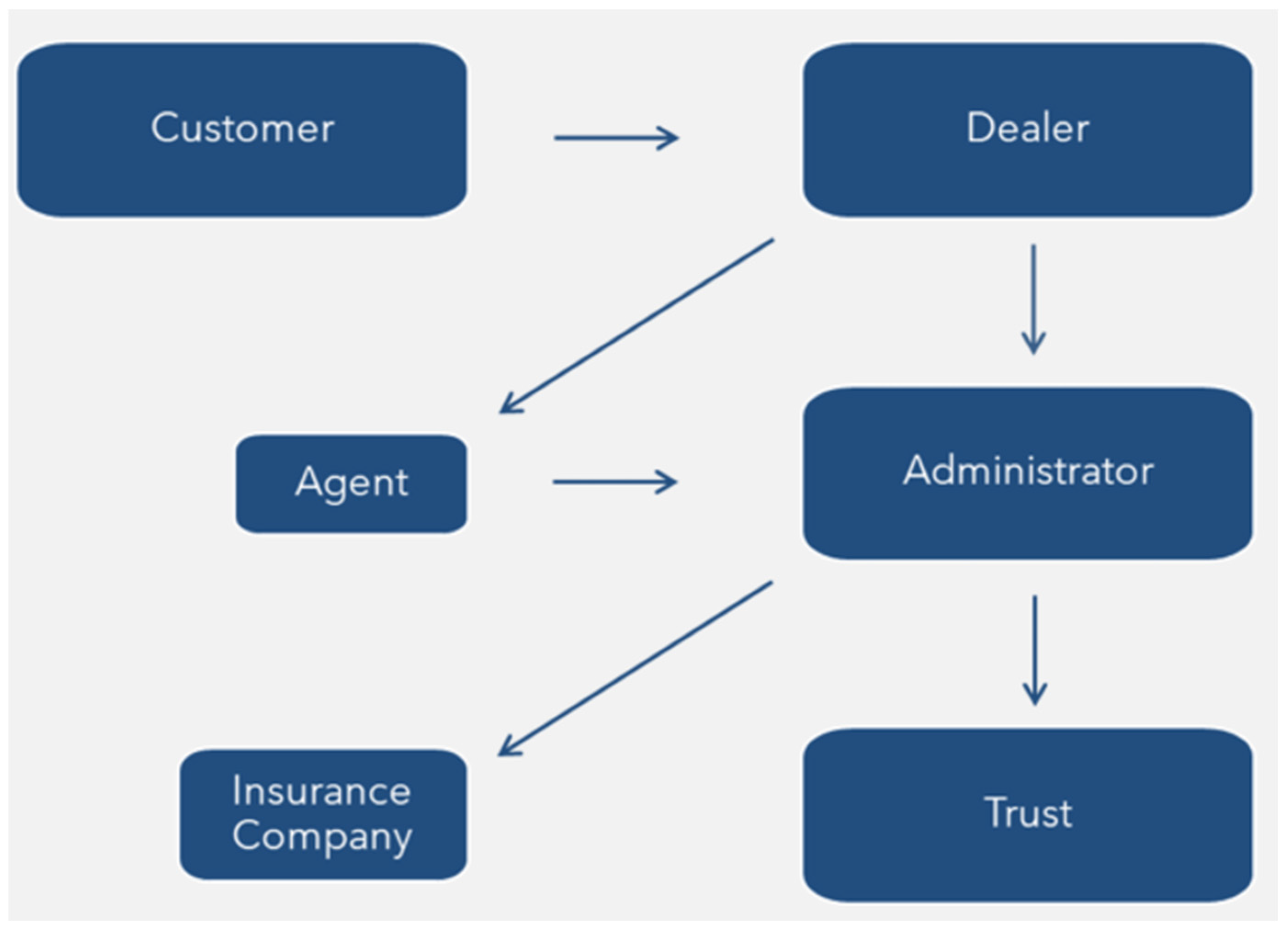
Franchised auto dealers in the USA sell a significant portion of service contracts. The structure of the market is complex—with the administrator at the center of the transaction—but awareness of other players of the cash flows and other providers is limited. Figure 2 provides a visual representation of initial cash flows from the purchase of a service contract.
A transaction will typically be structured as follows:
A Customer will purchase a service contract from a Dealership. The Dealership will be a client of the Administrator, which develops the product and services the claims and cancellations from the contract. Similar to traditional insurance, some service contracts are directly sold but many use Agents to distribute the product.
Legally, the contract can be a Dealer Obligor or Administrator Obligor. The obligor is the ultimate holder of the liability, though it is typically insured as described below. Third-party Administrator Obligors are the majority of the current market.
An example of a first-party Administrator Obligor structure is what is commonly referred to as a dealer-owned warranty company. The accounting treats the entire transaction as insurance for US Statutory financial statements and tax returns.16 This would require different treatment than the third-party Administrator Obligor for our example.
The Administrator acts as the central point of the transaction, as they control all the cash flows of the transaction.
A Trust, which is, in this case, structured as a lightly regulated insurance company with a non-US state domicile,17 assumes the risk. This is typically individually owned by a principal of the Dealership. The entire transaction is insured by a licensed US insurance company, either due to regulation or financing requirements from the lender. The Administrator takes a fee for claims handling, product development, and cancellation processing services.
The accounting and regulatory structure is different than traditional insurance. Unlike traditional insurance, the standards governing service contract prices do not include the typical insurance requirement that rates are not excessive, inadequate, or unfairly discriminatory. This is a fundamental standard embedded in state insurance laws.
In traditional insurance, the premium is remitted to the insurance company, and external providers such as agents and managing services are paid a percentage of the premium.
Service contracts are priced at the administrator level, and the dealer may, with exceptions, simply mark these up as with a typical retail sale. The administrator will receive the price they have determined. At that point, the administrator will split these proceeds and pay the agent, insurance company, and themselves.
The remaining amount will be put into a Trust. From this Trust, claims and cancels will be deducted as incurred. The owner of the Trust may only make withdrawals with the administrator’s approval. The typical requirement is that the Trust maintain slightly above 100% of the unearned premium and loss reserves in the Trust.
Any amount above this may be withdrawn as a profit distribution. Usually there is significant equity in the unearned premium reserve and the light capital requirements of the domicile do not require surplus to be maintained. The entire transaction is insured for completion under a contractual liability by a licensed insurance company. The risk to the insurance company is similar to bond insurance risk.
In some cases, the amounts paid under the service contract will be reimbursed by the insurance company. These transactions work in a similar way, but these service contract losses will appear on the licensed insurance company statement and ceded to the reinsurance company (Trust). These amounts will appear on Schedule F as unauthorized reinsurance, but the funding requirements will allow the insurance company to take credit for the transaction, with occasional Schedule F penalties when Trusts are not funded.18
In the hypothetical example below, a service contract is sold for $3000 at the time of vehicle purchase. Since this is financed with the vehicle, the payment increase in this case would likely be less than $50 a month depending on the term and interest rate on the loan.
Assume the various entities receive the following amounts shown in Table 10:

7.3.1. Service Contract Risk in the USA for Various Entities

Since these service contracts involve upfront payments for future services, accrual accounting is typically required to defer revenue and recognize it over the contract period (ASC 606 under GAAP as discussed above).
For an administrator, claims expenses must be reserved until expected payment or expected payment or cancellation.
Statutory insurance accounting, of course, requires an unearned premium, which is also recognized over the expected pattern of the claims.
ASC 606 standards require recognition at the time the service is performed. Since the service is the payment of the claim, entities will recognize revenue at the time of the estimated expected claim, which is the same as insurance companies.
Different rules may apply if the entity is not a party to the claim transactions. An example would be a dealership who sells contracts without a Trust.
Unlike insurance companies, some non-insurance entities such as Administrators may not be required to hold cash reserves. The deferred revenue is established as liability against the asset (the payment). These entities are more commonly evaluated under an EBITDA standard for valuation purposes.
  • Administrators:
For Administrators, this would be recognizing the $200 received at the beginning of the contract over the life of the contract. Since the administrator provides both cancellation and claims service to the customer, we will modify our revenue recognition pattern to include cancels.
We will define the ECC as the earned contract with cancels. By definition, this earning pattern will be slightly faster.
This would be accounted as:
  • P = Revenue the administrator receives for the contract ($200),
  • V = Months from inception date of contract to the valuation date ( V   term),
R e c o g n i z e d   R e v e n u e = P × i = 1 V E C C i .
  • Dealerships:
For Dealerships, the process is the same, except that the revenue should be recognized on the loss pattern only.
This would be accounted as:
  • M = Revenue the dealer receives for the contract ($1000),
  • V = Months from inception date of contract to the valuation date ( V   term),
R e c o g n i z e d   R e v e n u e = M × i = 1 V E C i .
  • Agents:
Since the Agent’s service to the customer is for the sale of the contract, these entities may recognize revenue immediately. Similar to other entities, they are subject to cancellation risk, and the forecasted amounts could be calculated as:
  • A = Revenue the agent receives for the contract ($100),
  • V = Months from inception date of contract to the valuation date ( V   term),
  • P = Premium placed into trust,
A g e n t   C a n c e l l a t i o n   F o r e c a s t = A P × i = v + 1 e F C E i .
A similar calculation could be done for a dealership cancellation liability as well.
  • Admitted Insurance Company:
Insurance companies are subject to US Statutory Accounting. These contracts are typically written as a “Failure-to-Pay”, where the risk of the failure of the obligor must be considered with financial risk of such a failure. If we assume that the failure rate of the obligor is constant throughout the contract, the proper proportional pattern would be the cumulative future claims at each evaluation. For example, a contract with 100% of the exposure at contact termination,19 a pro-rata earnings estimate would be appropriate. This recognizes the risk of obligor failure, which declines as the contract ages.
For insurance companies, the written premium ($40) would be recognized as:
  • P = Premium the insurance company receives for the contract ($40),
  • V = Months from inception date of contract to the valuation date ( V   term),
E a r n e d   P r e m i u m = P × ( i = 1 V F L i ) / ( i = 1 e F L i ) .
SSAP tests can be modified accordingly. There is no change to Test 1—Refund. Test 2 would be the formula above but including cancelations and other expenses. Test 3 would be based on actuarial judgment such as the expected loss ratio or specific information or conditions regarding obligor security.
Note that this might not change the booked reserve, as Test 1 will be higher than Test 2, but since this aggregation occurs at the company level, there may be other long-term unearned premiums (including first dollar transactions where all losses and cancels flow through the financials), which might change the indicated reserve.
  • Trust:
These trusts, as noted above, are subject to US Statutory Accounting.
For trusts, the earned premium ($1660) would be recognized as:
  • E T = Premium (“Reserve”) the trust receives for the contract ($1660),20
  • V = Months from inception date of contract to the valuation date ( V   term),
E a r n e d   R e s e r v e = E T × i = 1 V E C i .
Equity projections could be calculated as well.
  • US Insurance GAAP:
Outside of these structures including US insurance GAAP, there are transactions that would impact the asset side of the balance sheet. These would include “Deferred Acquisition Costs”.21
  • T A C   = Total Acquisition Costs,
  • e = Original term of contract,
  • e = Months from inception date of contract to the valuation date,
D A C = T A C × i = v + 1 e E C i .
As the chart above shows, service contracts in the USA can have a complicated structure. A single contract will have multiple parties of interest. Some entities such as Agents may face only cancellation risk and not claims risk.
Allocating by contract is more efficient than current practices. While current actuarial techniques can provide large entities with sufficient estimates, these methods cannot efficiently be extended to the other parties identified above.

7.3.2. Extended Warranty Special Case

In the USA, there are 2 distinct types of third-party sales, service contracts, and extended warranties. The distinction is legal. A third-party extended warranty has the same accounting, but there are key differences:
  • An extended warranty would be paid by the seller and included in the retail price. It is not an option—all customers who purchase the collateral will receive the extended warranty.
  • These extended warranties will fall under the jurisdiction of the Magnuson–Moss Warranty Act described above instead of the applicable Service Contract law. This allows for more restrictive language on coverage and the lack of cancellation provisions.
  • Because this product is “embedded” in the product, the knowledge of the extended warranty is lower in the consumer’s mind than a service contract. Therefore, claims will be lower than a service contract for the same coverage. This impact can be modelled using the techniques described above.
  • Extended warranties could be considered “first-party” risk—in that it is insuring the obligations of the seller, while a “service contract” would be “third-party” risk since it is insuring a sold product to a consumer. This may have an impact on the tax implications of how the transaction is characterized.
  • Another special case is the “Lifetime Warranty”, which does not have an expiration date. In order to account for this, an assigned term of perhaps 20 years would be assigned to these contracts. These types of contracts will typically have few claims in the tail. This is a balance of capturing all the exposure on the contracts and the need to expire these contracts at some point. In any event, systems should allow for the occasional claim on an expired contract.

8. Monthly Contracts and Customer Lifetime Value (CLV)

The scope of the KB Method technique would be all service contracts sold with a term greater than 1 month for the repair, maintenance, or accidental damage of a covered item.
For terms of 1 month, the techniques could technically still be utilized for accounting purposes; however, the differences between the KB Method and a “straight-line accrual” method would be immaterial.
Monthly contracts are common where the contract is sold after the purchase of the covered item, or the covered item is subject to a subscription service.
In developing a CLV, we will consider the future probabilistic revenue combined with the projection under the KB Method which will consider renewal age among other factors.
The large telephone manufacturers and telecommunication providers dominate the monthly service contract market and likely have sophisticated lifetime models.
However, this CLV implementation may be more appropriate for the relatively smaller programs largely consisting of vehicles and household goods. These programs are typically service contracts related to affinity groups with Triple A an example.
Direct service contracts are also available. These are now marketed by traditional in-bound marketing.22
In order to analyze these contracts more effectively, let us change the definition of age to include the renewals, and the age becomes the number of months since the initial contract purchase.
We will define the Future Negative Cash Flows Related to Claims and Cancels ( F L C M ) as the expected amount of claims, cancels and variable expenses for monthly contracts over the lifetime of the contract as:
F L C M = v + 1 t F L C M i .
The F L C M is analogous to the F L C as defined above with some key differences discussed below.
In modelling the cost per exposure, the age factor will identify the impact of renewals on contracts, which could show varying measures depending on how the program is designed. Products could show decreasing or increasing claims with renewal age.
The exposures ( A F E ) as defined above would be reduced by a retention model for future exposures.
A simple age-to-age model of retention can be easily developed. There are also a wide variety of statistical and machine learning techniques on retention as well as methods to improve it. These results could be easily used to form the A F E .
Projections from the modified KB method are modified from “Future Liabilities” to “Future Negative Cash Flows Related to Claims and Cancels”. This should be adjusted for other expenses for active service contracts such as claims handling and payment processing expenses.
Combined with the future revenue estimated from the selected retention model, the CLV can be calculated.
CLV estimates could be used for a variety of applications for service contract writers. These include forecasting, accounting accruals, and collateralization of acquisition costs.

9. Conclusions

The Kerper–Bowron Method provides a foundational advancement in service contract claim estimation and accounting. Contributions include:
  • Functional equivalency to the challenge of exact Solvency II equivalence for finite risks.
  • Replacement of aggregate approximations with auditable, contract-specific projections.
  • Transformative implications for reserving accuracy, compliance, and capital efficiency.
  • Practical applications extend to real-time equity visibility, automated regulatory reporting, and potential lending solutions within reinsurance trusts.
  • Identified extensions of the KB Method including customer lifetime value models as well as other applications outside the scope of this paper including manufacturer’s warranty accruals
Future work includes comprehensive empirical validation across diverse contract types and jurisdictions, integration with AI-driven forecasting, and exploration of broader applications in the service contract and warranty space.
The KB Method provides a statistical estimate for customer-level transactions. Another analogous process is CLV accounting, as discussed above but in general concepts beyond service contracts.
CLV accounting estimates the total revenue a business expects from a customer over their relationship, using statistical models like regression analysis, survival analysis, or Markov chains. It is widely used in industries like retail, e-commerce, and subscription-based services.
The KB Method is different than CLV accounting since these estimates are less dependent on company performance (i.e., maintaining an acceptable subscription product). Instead of estimating future revenue, the KB Method estimates future expenses, i.e., claims and cancels.
This work bridges theoretical rigor and practical relevance, offering a powerful tool for modern risk management.

10. Patents

The Kerper–Bowron Method described herein is patent-pending (Kerper and Bowron 2025).

Author Contributions

Conceptualization, J.K. and L.B.; Methodology, J.K. and L.B.; Software, J.K. and L.B.; Writing—original draft, J.K. and L.B.; Writing—review & editing, J.K. and L.B. All authors have read and agreed to the published version of the manuscript.

Funding

This research received no external funding.

Data Availability Statement

The data presented in this study are available in Transportation Secure Data Center [2004–2006] (https://www.nrel.gov/transportation/secure-transportation-data/tsdc-puget-sound-traffic-study, accessed on 23 May 2025). In addition, there are illustrative examples that use hypothetical data generated for demonstration purposes.

Conflicts of Interest

John Kerper and Lee Bowron are inventors on US Provisional Patent Application No. 63/858,053 related to the methods described in this paper and are co-founders of Kerper and Bowron LLC and Irish Trinity LLC, which may commercialize the technology. The authors have no other competing interests to declare.

Appendix A. Flow Chart of the Kerper–Bowron Method

Start
Collect Point-of-Sale Data and Claims
(term, mileage eligibility, coverage, deductible, vehicle profile, price, claim payment, part, date of loss, date of payment, and other relevant factors)
Calculate Exposures
(lognormal to truncate exposures for time and mile limitations)
Select Study Period
(calculate exposures and develop losses to ultimate)
Develop Model
(GLM or other model, testing significance, identifying covariances)
Calculate Future Loss and Cancel Estimate
(Develop future exposures adjusted for cancellations, estimate future cancellations, trend, and seasonality)
Compute Contract-Level Estimates
(losses, unearned premium, equity emergence)
Apply Regulatory Alignments
(Solvency II, IFRS 17, ASC 606, etc.)
Output: Auditable Cash Flows and Accounting Entries
End

Appendix B. Goodness of Fit Tests for Lognormal Distribution
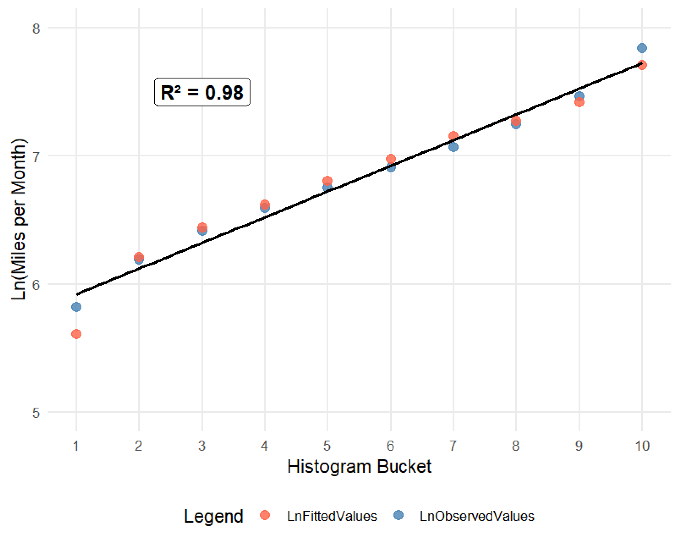
Figure A1. Observed versus fitted Ln(miles per month) by histogram bucket.
Risks 14 00044 g0a1

Appendix C. Puget Sound Data Process

1.
The Puget Sound Study data can be shown to produce a distribution of individual driving habits by performing the following steps: Download the raw data from Puget Sound Study (2004–2006) 2004–2006 Puget Sound Traffic Choices Study|Transportation Secure Data Center|NREL.
2.
Only the data from extracted table v_gpstrips were used.
3.
A total of 64 records attributed to 9 different SampNos were removed due to data insufficiencies. Removing all records with these SampNos will remove those 64 records: 30696, 43406, 43420, 43427, 43428, 43446, 43451, 43457, and UPDAT.
4.
Column ‘bktp_mt_total’ is summed by sample number to calculate the total miles driven during the study for each sample number and defined as ‘Miles.’
5.
The minimum of ‘bktp_start_date’ and maximum of ‘bktp_end_date’ of each sample number rounded down to zero digits is selected to establish a start and end date of study participation for each SampNo. Note—rounding down to zero digits is important because the dates in the data are stored in a date-time format. Calculation results will differ if time is not removed.
6.
The length of participation in the study in years for each SampNo was then calculated using this formula.
P a r t i c i p a t i o n = E n d   D a t e S t a r t   D a t e ÷ 365.25 .
7.
Finally, the Miles per Month is calculated and used for the lognormal definitions above. This should result in monthly driving patterns for 319 drivers.
M i l e s   p e r   M o n t h = M i l e s ÷ P a r t i c i p a t i o n ÷ 12 .

Notes

1
A somewhat common exception would be the creation of a Premium Deficiency Reserve (“PDR”). The PDR occurs when the forecast liability is greater than the unearned premium. These numbers could easily be calculated using the techniques developed below.
2
In order to determine whether a service contract on a vehicle has any remaining manufacturer’s warranty, it is necessary to know both the current odometer reading on the vehicle and the in-service date of the vehicle. While the odometer reading is virtually universally known, accurate information on the in-service date is difficult to determine.
3
The “Reverse Rule-of-78s” is the inverse of the “Rule-of-78s”, which earns contracts on a “sum-of-the-digits” method. The “Rule-of-78s” was developed to allocate interest and principal on loans beginning in the early 20th century. Interest would be allocated on the sum-of-the-digits basis. For a 12-month loan, interest for the second month would be allocated as (1 − (10 × 11))/(12 × 13) or 29.5% of the total interest for the second month. The method is favorable to the lender. Due to this and technological advancements, this method has fallen out of favor. The “Reverse Rule-of-78s” counts from the beginning, so the number 11 in the example above is changed to 2. This method has increasing earnings levels for each month. For new cars, this is not correct. There is virtually no earned premium in the second month of a new vehicle, as a negligible number of vehicles have exceeded the mileage under a new vehicle warranty. In addition, many drivers will expire their contract by exceeding the service contract mileage limitations before the time limitations. Because of this, this method has fallen largely out of favor but still remains on a few older programs and systems.
4
In the authors’ opinion, the usage of separate frequency and severity estimates is fundamentally flawed for service contract analysis due to the frequently observed high negative correlation between frequency and severity depending on a variety of factors. For example, if a service contract provider (Administrator) introduces a new maintenance benefit, the observed frequency of the book will increase (perhaps dramatically) while the severities will fall. Another common issue is powertrain coverage, which limits coverage to engine components. These exposures will have lower frequencies and higher severities. The use of loss costs or pure premiums eliminates this noise effectively.
5
The General Data Protection Regulation, adopted in 2018, has limited participation to approximately 30% of drivers. See ISG, “Technology That Creates Flood of Data Can Also Help Actuaries Make Better Decisions” (Winkler 2021). EV reliability and EV battery life remains an open question. Many administrators are seeking to add EV Battery coverage in the USA. There are proposed repairs that may not require a full battery replacement. EV Battery warranties are typically 8–10 years with high mileage limits. There is a lack of data on battery life after the warranty due to the relatively low number of EVs with expired battery warranties. Battery replacement is an expensive repair, with reports of some EV replacements reaching $20,000 or more. There is also the question of “betterment”, as a new battery could almost be considered a new engine. Traditional battery coverage is not offered on VSCs without a maintenance component because it is considered a wear-and-tear item.
6
Mileage is captured upon cancellation or claim. Since the cancellation date and loss date are also included, mileage patterns can easily be estimated from an existing book.
7
Historical “system reports” were almost always segregated by policy year.
8
Most service contracts are based on term miles, which is miles in addition to starting miles. A significant minority use the odometer reading as the expiration miles. For example, a 5 year/75,000 mile contract with 20,000 miles at purchase would expire at 95,000 miles on term mile contract and 75,000 miles on an odometer mile contract. For the purpose of this paper, we consider all miles to be term miles. These can easily be calculated for odometer expiration contracts by taking the odometer expiration miles less that initial odometer reading.
9
The structure of the VSC industry in the USA often includes flat additions for the Dealer Markup, Agent Fee, and Administrator Fee rather than a percentage. Due to this, any options such as coverage and deductible will be biased towards the most comprehensive coverage (higher term, lowest deductible, highest coverage) since the consumer will only pay for the increase in the portion in expected losses.
10
The amount retuned on cancellation (60–80% of unearned) may be similar to the future loss ratio, which will have minimal impact on the overall liability but will impact the cash flow, as the cancellation will occur before the projected claims. Most cancels occur early in the contract, and “flat cancels”, which are cancels for a full refund typically occurring without a claim and in the first 30 days, are removed from the analysis.
11
VSCs are typically cancelled on the greater of months and miles, without regard to the underlying manufacturer’s warranty. In most cases, this will result in a refund less than the underlying unearned premium reserve. In any case, a factor can be calculated based on the average refund/unearned premium observed. If telematics or other sources of contract mileage data are available, a better estimate can be formed.
12
For example, televisions have historically been more dependable than refrigerators or washing machines.
13
EVs are getting more reliable, but they still lag behind hybrids and gas-only cars.
14
The Solvency Capital Requirement (SCR) is defined in Articles 100–127 of the Solvency II Directive (2009/138/EC) as the capital needed to cover a 99.5% worst-case scenario over one year, calculated using the standard formula or an approved internal model.
15
For example, Dell Technologies’ total revenue for fiscal year 2025 (ended 31 January 2025) was $95.6 billion. An undisclosed amount is due to service contracts, but this revenue likely exceeds 3 billion.
16
US statutory accounting does not allow for the amortization of acquisition costs. Since this type of structure has high acquisition costs and long terms, it produces significant statutory income losses in the first few years of the contract, followed by high profits in the latter part of the term.
17
The most popular domiciles for these companies is the Turks and Caicos and the Delaware Tribe of Kansas, with occasional companies in other offshore domiciles such as the Seychelles. Offshore companies will file a 953(d) election, which elects US tax treatment of the transaction. Regardless of domicile, the financial assets remain in the USA.
18
There is some confusion over nomenclature in the industry in this area. Many of these entities are known as “reinsurance companies”. A minority function as reinsurance companies, with all funds passing through an “A-rated” company and fully reinsured to these companies. However, the majority directly assume the risk.
19
An example would be “Lease Wear and Tear”, which covers cosmetic damage to a returned leased vehicle. The majority of these leased vehicles will be returned near or at the lease end date.
20
Industry nomenclature typically replaces “premium” with “reserve” for these entities.
21
Deferred Acquisition Costs (DAC) refer to certain costs incurred by an insurance company that are directly related to acquiring or renewing insurance contracts. These costs are capitalized and amortized over the period in which the related premiums are earned, rather than being expensed immediately, to align with the revenue recognition principle under GAAP.
22
The topic of robocalls and direct-marketed contracts has filled the authors’ ears at a few dinner parties. While these types of calls were always illegal, enforcement was lacking until 21 July 2022, when an FCC order (File No. EB-TCD-21-00031913) effectively ended the practice by a heavy sanction action. Therefore, the calls have stopped for now. Despite the noise, direct marketed VSCs have always had an immaterial market share. Another interesting facet of direct marketed service contracts is the term of the contracts sold. VSCs are traditionally sold as longer terms because they are financed with the loan for the underlying vehicle. Direct-marketed VSCs could have been offered with a monthly term, but industry systems and tradition allowed for longer term contracts. Finance companies technically financed these contracts, but consumers who failed to pay did not owe further obligation since the refund generated by a cancellation was typically sufficient to satisfy the balance of the “loan”. The acquisition costs were funded immediately but the cancellation ratio was very high, as many customers only used or needed this product for a few months. Unfunded refund liabilities led to well-documented defaults such as US Fidelis (Wentzville, MO, USA). While these practices were deficient, the need to fund the acquisition cost for a direct-marketed service contract is a legitimate concern for these entities, which these techniques can address.

References

  1. Barry, Keith, Anita Lam, and Steven Elek. 2025. Hybrids Are Still the Most Reliable Cars, CR Survey Shows. Available online: https://www.consumerreports.org/cars/car-reliability-owner-satisfaction/electric-vehicles-are-less-reliable-than-conventional-cars-a1047214174/?msockid=2f5441b7079c6f2712df540506fc6e82 (accessed on 9 February 2026).
  2. Bashina, Asya. 2025. ASC 606 Implications for Warranties. Available online: https://www.leapfin.com/blog/accounting-for-warranties-under-asc-606 (accessed on 9 February 2026).
  3. Bertolini, Michelle. 2007. Service-Warranty Companies—The Hybrid of the Insurance Industry. Available online: https://www.thetaxadviser.com/issues/2007/jul/service-warrantycompanies-thehybridoftheinsuranceindustry/ (accessed on 9 February 2026).
  4. Breitenstein, Jennifer. 2020. Product vs. Extended Warranties: Difference Revealed. OnPoint Insurance Technology and Warranty Services 2020. Available online: https://www.onpointwarranty.com/about-us/blog/product-vs-extended-warranties (accessed on 9 February 2026).
  5. Brown, Chris. 2025. The History of Extended Car Warranties. Available online: https://www.endurancewarranty.com/learning-center/extended-warranty/history-of-extended-car-warranties/ (accessed on 9 February 2026).
  6. Casualty Actuarial Society. 2025. IFRS-17—Microlearning Series. Available online: https://www.pathlms.com/cas/courses/66621# (accessed on 9 February 2026).
  7. Diamantoukos, Christopher. 1991. Discussion of Paper Published in Volume LXXVI Exposure Bases Revisited. Arlington County: Casualty Actuarial Society. [Google Scholar]
  8. European Parliament. 2009. Directive 2009/138/EC of the European Parliament and of the Council of 25 November 2009 on the Taking-Up and Pursuit of the Business of Insurance and Reinsurance (Solvency II). Available online: https://www.legislation.gov.uk/eudr/2009/138/contents (accessed on 9 February 2026).
  9. Extended Warranty Profits. 2004. Warranty Week. Available online: https://web.archive.org/web/20241231093435/https://www.warrantyweek.com/archive/ww20041026.html (accessed on 9 February 2026).
  10. FASB. 2014. Revenue from Contracts with Customers. ASC 606. Norwalk: Financial Accounting Standards Board. [Google Scholar]
  11. Federal Trade Commission. 2023. Extended Warranties and Service Contracts. Available online: https://consumer.ftc.gov/articles/extended-warranties-and-service-contracts (accessed on 9 February 2026).
  12. Financial Accounting Standards Board. 1990. FTB 90-1. Available online: https://fasb.org/page/document?pdf=ftb+90-1.pdf&title=FTB+90-1+(AS+ISSUED) (accessed on 9 February 2026).
  13. Grandview Research. 2025. Extended Warranty Market Size, Share|Industry Report 2026–2033. Available online: https://www.grandviewresearch.com/industry-analysis/extended-warranty-market-report (accessed on 28 January 2025).
  14. Hayne, Roger. 2007. Extended Service Contracts, an Overview. Variance 1. Available online: https://variancejournal.org/article/141777-extended-service-contracts-an-overview (accessed on 9 February 2026).
  15. Highway Statistics. 2005. Table VM-1. Available online: https://www.fhwa.dot.gov/policy/ohim/hs05/ (accessed on 9 February 2026).
  16. ISAB. 2017. IFRS 17 Insurance Contracts. London: International Accounting Standards Board. [Google Scholar]
  17. Jiang, Haoran, and Haylie Dayley. 2020. Warranty Obligations in ASC 606. Available online: https://www.revenuehub.org/article/warranty-obligations (accessed on 9 February 2026).
  18. Kerper, John, and Lee Bowron. 2007. An Exposure Based Approach to Automobile Warranty Ratemaking and Reserving. Casualty Actuarial Society Forum 2007. Arlington County: Casualty Actuarial Society. [Google Scholar]
  19. Kerper, John, and Lee Bowron. 2025. Systems and Methods for Service Contract Loss Estimation and Accounting. U.S. Patent 63/858,053, August 5. [Google Scholar]
  20. Meyers, Glenn. 2009. Predictive Modeling with the Tweedie Distribution. In CAS Annual Meeting. Boston: Casualty Actuarial Society. [Google Scholar]
  21. National Laboratory of the Rockies. 2004–2006. Puget Sound Traffic Choices Study. Available online: https://www.nlr.gov/transportation/secure-transportation-data/tsdc-puget-sound-traffic-study (accessed on 9 February 2026).
  22. Pope, Nat, Chiharu Ishida, and Peter Karufman. 2022. The Service Contracts Model Act: A Quarter Century and Counting—What Now? Available online: https://content.naic.org/sites/default/files/the-service-contracts-model-act-jir-2022-05.pdf (accessed on 9 February 2026).
  23. U.S. Bureau of Labor Statistics. 2025. Consumer Price Index for All Urban Consumers: Motor Vehicle Maintenance and Repair in U.S. City Average. Available online: https://fred.stlouisfed.org/series/CUUR0000SETD (accessed on 9 February 2026).
  24. Warranty Conference. 2005. Warranty Week. Part 5. Available online: https://web.archive.org/web/20240617110226/https://www.warrantyweek.com/archive/ww20050405.html (accessed on 9 February 2026).
  25. Winkler, Dennis. 2021. Technology That Creates Flood of Data Can Also Help Actuaries Make Better Decisions. Available online: https://isg-one.com/articles/technology-that-creates-flood-of-data-can-also-help-actuaries-make-better-decisions (accessed on 9 February 2026).
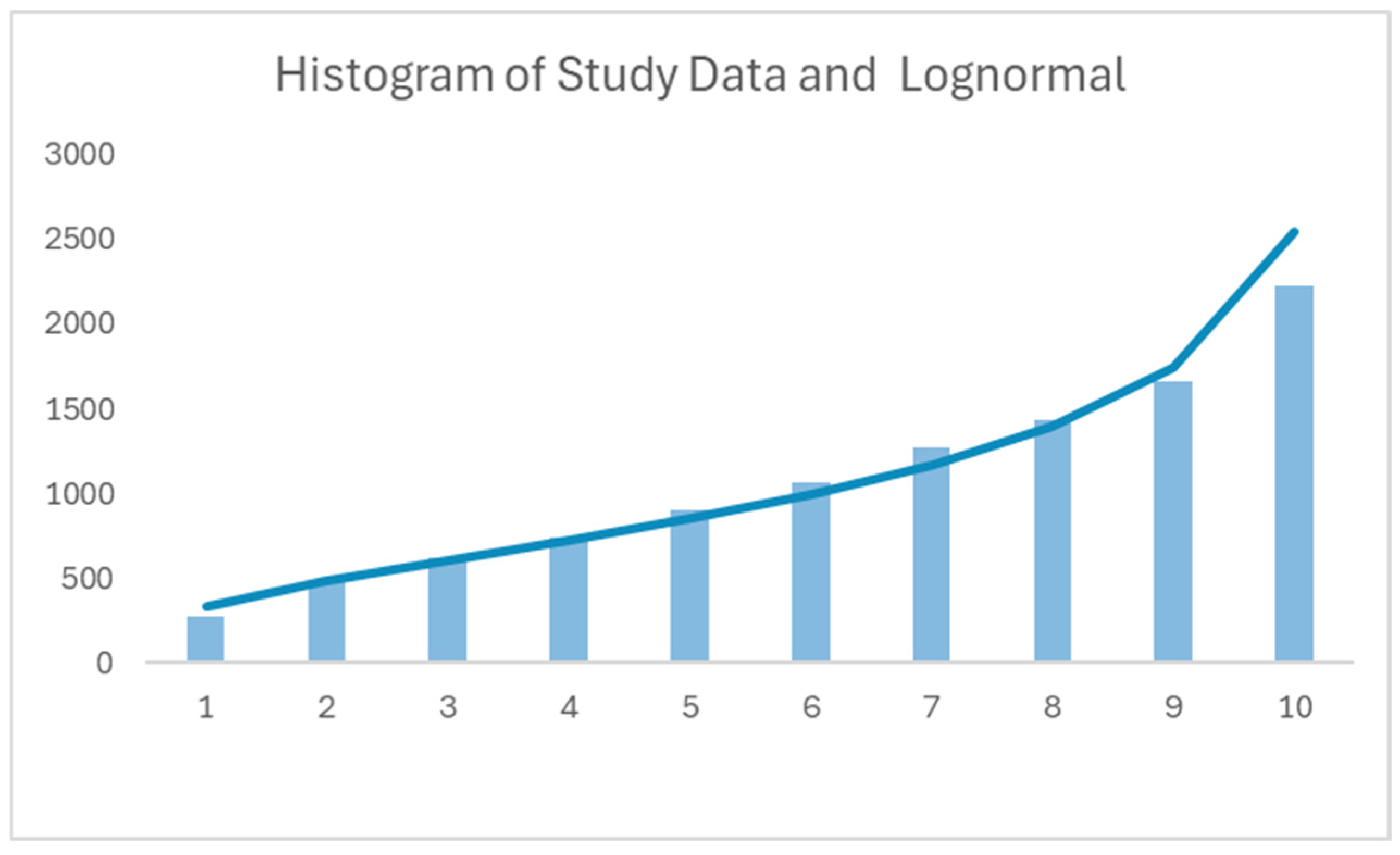
Figure 1. Histogram of study data overlayed with the lognormal curve.
Risks 14 00044 g001
Figure 2. Initial revenue allocation for a service contract.
Risks 14 00044 g002
Table 1. Examples of earnings curves for a 36 month VSC contract.
MonthPro-RataReverse Rule of 78sExperience Based
00.00000.00000.0000
10.02780.00150.0387
20.05560.00450.0767
30.08330.00900.1138
40.11110.01500.1502
50.13890.02250.1859
60.16670.03150.2209
70.19440.04200.2552
80.22220.05410.2888
361.00001.00001.0000
Table 2. Pure premiums by valuation date.
Pure Premiums − Paid Losses/In-Force Contracts
by Age
PolicyPolicy
YearQuarter369121518212427303336
20191ST26.8325.1423.9922.2019.4218.0916.5917.6515.5614.8815.2613.80
20192ND23.7425.6325.5921.9120.8221.2016.4516.7516.4515.4514.6214.43
20193RD27.1826.1223.6720.1319.2618.9719.1617.2815.6715.9914.5314.09
20194TH28.5523.9125.9621.1620.7118.6118.2415.6917.8616.4013.6913.77
20201ST24.2125.5425.9323.7121.9319.3719.4319.1317.8015.6915.3114.25
20202ND25.9627.4824.5323.3720.5421.4118.4617.2817.9116.7415.0713.63
20203RD25.7726.1526.0323.0820.8420.2119.0417.3215.5214.5613.5012.99
20204TH28.3927.9522.8924.0222.7319.7618.4519.1215.7215.8116.2513.23
20211ST26.1127.9525.8222.5623.2322.2920.6716.6216.5315.4613.5815.32
20212ND28.1027.2926.1623.8722.7221.6220.7418.6318.1514.5114.3314.53
20213RD25.2523.7523.1724.3822.5619.9818.1816.7518.0114.6215.3913.22
20214TH29.5027.8423.3123.3021.7321.2019.3817.7218.7316.3514.7715.13
20221ST28.1828.8925.2525.9022.5121.5018.7820.1618.1416.0814.9814.29
20222ND25.8728.0724.9123.1521.6323.2218.3918.4818.5017.4916.92
20223RD26.7128.7825.2325.0123.8222.2119.9219.8518.4517.96
20224TH31.8128.4727.2026.1523.6622.9820.7220.1118.48
20231ST28.0126.5924.9625.2621.0620.2721.8818.61
20232ND32.4329.0026.8823.4421.2020.7222.15
20233RD29.2630.0727.0826.3925.3722.65
20234TH29.1530.0528.9522.7723.69
20241ST27.6128.4929.1823.28
20242ND33.1331.1628.31
20243RD33.0328.09
20244TH32.46
Exponential Fit30.4228.8326.4224.1322.7021.4320.1118.3117.6715.4914.2913.25
Selected 30.4228.8326.4224.1322.7021.4320.1118.3117.6715.4914.2913.25
Table 3. Indicated pure premium.
(1)(2)(3)(4)(5)
InterpolatedIncrementalCumulative
Prior PeriodFuture PeriodMonthlyEarningsEarnings
MonthPure PremPure PremPure PremCurveCurve
0 30.420.000.0000.000
1 30.4230.420.0390.039
2 30.4229.890.0390.078
330.4228.8330.420.0390.117
430.4228.8329.890.0390.155
530.4228.8329.360.0380.193
628.8326.4228.830.0370.230
728.8326.4228.030.0360.267
828.8326.4227.230.0350.302
926.4224.1326.420.0340.336
1026.4224.1325.660.0330.369
1126.4224.1324.890.0320.401
1224.1322.7024.130.0310.432
1324.1322.7023.650.0300.463
1424.1322.7023.170.0300.492
1522.7021.4322.700.0290.522
1622.7021.4322.280.0290.550
1722.7021.4321.850.0280.579
1821.4320.1121.430.0280.606
1921.4320.1120.990.0270.633
2021.4320.1120.550.0260.660
2120.1118.3120.110.0260.686
2220.1118.3119.510.0250.711
2320.1118.3118.910.0240.735
2418.3117.6718.310.0240.759
2518.3117.6718.100.0230.782
2618.3117.6717.890.0230.805
2717.6715.4917.670.0230.828
2817.6715.4916.940.0220.850
2917.6715.4916.220.0210.871
3015.4914.2915.490.0200.891
3115.4914.2915.090.0190.910
3215.4914.2914.690.0190.929
3314.2913.2514.290.0180.947
3414.2913.2513.940.0180.965
3514.2913.2513.590.0180.983
3613.25 13.250.0171.000
Total775.801.000
Table 4. Exposure base for different lines of business.
Line of BusinessExposure Base
HomeownersEarned House Year
GL (Premises)Square Footage
Workers’ CompPayroll
Commercial AutoEarned Car Year
Inland MarineProperty Value
UmbrellaUnderlying Policy Premiums
Special EventTime-Based Exposure (Hours/Days)
Apt/Condo LiabilityNumber of Units
Product LiabilityGross Sales/Revenue
Table 5. Summary of bumper-to-bumper and powertrain warranties for major makes.
MakeBumper-to-Bumper WarrantyPowertrain WarrantyLocations
Toyota3 years/36,000 miles5 years/60,000 milesJapan
Ford3 years/36,000 miles5 years/60,000 milesUnited States
Chevrolet3 years/36,000 miles5 years/60,000 milesUnited States
Honda3 years/36,000 miles5 years/60,000 milesJapan
Nissan3 years/36,000 miles5 years/60,000 milesJapan
Hyundai5 years/60,000 miles10 years/100,000 milesSouth Korea
Kia5 years/60,000 miles10 years/100,000 milesSouth Korea
Jeep3 years/36,000 miles5 years/60,000 milesUnited States
Ram3 years/36,000 miles5 years/60,000 miles (gas)United States
GMC3 years/36,000 miles5 years/60,000 milesUnited States
Subaru3 years/36,000 miles5 years/60,000 milesJapan
Mazda3 years/36,000 miles5 years/60,000 milesJapan
Table 6. Key parameters.
Average Annual MilesStd Dev ln(Miles per Month)Mean ln(Miles per Month)
13,0830.626.83
Table 7. Lognormal assumptions.
Starting Odometer850
Mean ln(Miles per Months)6.83
Std Dev ln(Miles per Months)0.62
Service Contract Months96
Service Contract Miles96,000
Manufacturers Warranty Months36
Manufacturers Warranty Miles36,000
Table 8. Calculation of service contract exposure (B–D).
Starting Mileage850
Warranty Mileage Term36,000
Warranty Mileage Remaining35,150
(A)(B)(C)(D)(E)(F)
Miles Driven inRemainingMiles Driven inRemainingService
Month to ExceedPercent inMonth toPercent inContractAdjusted
MonthService ContractService ContractExceed WarrantyWarrantyExposureExposure
0 to 1192,0001.000070,3001.00000.00000.0000
1 to 264,0001.000023,4331.00000.00000.0000
2 to 338,4001.000014,0601.00000.00000.0000
3 to 427,4291.000010,0430.99990.00010.0001
4 to 521,3331.000078110.99970.00030.0003
29 to 3032540.979711920.66070.31900.2935
30 to 3131480.976911520.64060.33630.3425
31 to 3230480.973911160.62080.35300.3480
32 to 3329540.970610820.60130.36930.3761
33 to 3428660.967210490.58220.38490.3794
34 to 3527830.963510190.56350.40000.4074
59 to 6016130.81785910.00000.81780.8329
60 to 6115870.81055810.00000.81050.7989
61 to 6215610.80325720.00000.80320.8181
62 to 6315360.79595620.00000.79590.7844
63 to 6415120.78855540.00000.78850.8031
64 to 6514880.78115450.00000.78110.7955
89 to 9010730.59613930.00000.59610.5484
90 to 9110610.58913880.00000.58910.6000
91 to 9210490.58223840.00000.58220.5738
92 to 9310380.57533800.00000.57530.5859
93 to 9410270.56843760.00000.56840.5602
94 to 9510160.56163720.00000.56160.5720
95 to 9610050.55483680.00000.55480.5651
Table 9. Service contract exposure by valuation date.
Contract Start Date7 September 2026
Term96
Contract Exp Date7 September 2034
(A)
Valuation DateService Contract Exposure
30 September 20260.0000
31 October 20260.0000
30 November 20260.0000
31 December 20260.0000
31 January 20270.0002
28 February 20270.0006
31 March 20290.3385
30 April 20290.3441
31 May 20290.3724
30 June 20290.3758
31 July 20290.4040
31 August 20290.4188
30 September 20310.8006
31 October 20310.8198
30 November 20310.7861
31 December 20310.8048
31 January 20320.7972
29 February 20320.7388
31 March 20340.6016
30 April 20340.5754
31 May 20340.5875
30 June 20340.5618
31 July 20340.5735
31 August 20340.5666
30 September 20340.1276
Table 10. Hypothetical revenue from a service contract.
Retail Price3000
AmountRemaining
EntityReceived Amount
Dealership10002000
Agent1001900
Administrator2001700
Insurance Company401660
Trust16600
Disclaimer/Publisher’s Note: The statements, opinions and data contained in all publications are solely those of the individual author(s) and contributor(s) and not of MDPI and/or the editor(s). MDPI and/or the editor(s) disclaim responsibility for any injury to people or property resulting from any ideas, methods, instructions or products referred to in the content.