Using Human Assessment and GC-MS to Identify Potential Use Cases for Evaluating Food Condition with Gas Sensor Systems

Abstract

Technological solutions might be of great importance for reducing food waste. In the scope of this article, gas sensor systems for assessing the edibility of food have been studied, which can help to avoid food losses by suggesting consumption before spoilage or by separating infected fruits from fresh ones. Several series of measurements with various foodstuffs were conducted to develop methods that enable the identification of possible use cases in which gas sensors could be used to assess food condition as well as methods to calibrate such sensor systems. This paper presents results for oranges as an important target for grocery stores. The fruit headspace was measured by gas sensors, reference data were acquired using human assessment (appearance, odor, edibility) and gas chromatography–mass spectrometry (GC-MS) analysis. Data evaluation shows correlations between the performance of individual sensors for a technical assessment of fruit condition with marker substances identified by GC-MS, e.g., limonene for damaged oranges. Models were derived that are, in general, able to quantify the edibility or to classify defects/mold, but limitations in the applicability/transferability, e.g., between orange varieties, were also identified. With the knowledge gained, important steps could be taken towards an application-oriented setup, and recommendations regarding the sensors used, food trained, and calibration methods applied are derived.

1. Introduction

Reducing food waste is of high importance considering the economic and ecological effects of unnecessary use of resources (land, water, carbon dioxide emissions, etc.). About 20% [1,2] to up to one third [3] of food production is lost or wasted, depending on the data sources used, the assumptions made, and the region covered (e.g., the EU vs. globally). Typically, in industrialized regions, consumer-related food waste contributes to approx. 50% or more of the losses of cereals and dairy products, and, if distribution is added, of fruits and vegetables as well [3]. At the same time, vegetables, fruits, cereals, and meat account for the largest share of food waste in general as well as at the consumption level [1]. At least 50% of this food waste is regarded as edible and, thus, avoidable in every step of the food supply chain [2] and for every food category at the consumption level [1]. The consumption phase accounts for the largest amount of the overall carbon footprint of food waste, as food products at that stage went through the whole food supply chain, adding additional emissions [4]. Thus, reducing food waste at the consumption level is especially interesting, but significant saving potential exists at every stage of the food supply chain, and cereals, meat, as well as fruits and vegetables are of major interest.

The reasons for consumer-related food waste, i.e., food waste in households and, to a certain extent, food waste in retailing, as the latter is highly affected by the consumers’ behavior, are diverse, from poor planning, wrong or limited understanding of date labels (e.g., best before), shelf-life, and food safety to cooking, storing, or managing issues, but they also include insufficient awareness and understanding regarding food waste [5,6,7]. Accordingly, possible measures for reducing food waste are manifold, including the optimization of food labeling and education of consumers [6,8,9], but technological solutions, e.g., providing real-time feedback, seem promising as well.

Reduction of food waste by technological solutions is only feasible where the actual state of the food causes its disposal. Thus, the assessment of the food’s condition, i.e., its degree of ripeness, freshness, spoilage, or damage, would be an interesting target for sensor-based devices. Such a device could support the consumer to decide whether a food product is still safe to consume; similarly, it could support storage and fruit display management in retailing. Quality estimation or spoilage detection by measuring volatile compounds in the headspace of food has been extensively discussed in the literature starting many years ago, including the use of the then just emerging so-called electronic noses [10,11]. There are numerous examples of gas sensors or sensor systems developed for the detection of gases that are relevant to monitoring ripeness (e.g., ethylene [12]), spoilage (e.g., hydrogen sulfide and/or ammonia [13,14,15]), or storage conditions (e.g., carbon dioxide) [16]. On the other hand, gas-specific sensors are not essential for such devices; instead, several non-specific gas sensors, e.g., metal oxide semiconductor (MOS) gas sensors, can be combined in a sensor array with appropriate signal processing to discriminate between gases or odors. This stems from comparison with the mammalian olfactory system as a natural reference as first demonstrated by Persaud and Dodd [17]. Thus, a complementary approach is the use of several sensors—sensors of different sensing material, doping, and/or sensors set to different temperatures—in a sensor array, which is a key feature in many experimental and commercial electronic noses as it enables pattern recognition [18,19]. Similarly, a virtual sensor array can be implemented by dynamically operating a single sensor element, e.g., via a cyclic change of the sensor temperature to different values (temperature-cycled operation, TCO), which can enhance selectivity and sensitivity, but also stability [20]. In both cases, comprehensive calibration and pattern recognition are essential for successful processing and interpretation of the sensor signals.

Despite these already existing technologies and available feasibility studies, only a few sensor-based systems for monitoring food conditions are available on the market, and the underlying reasons are probably manifold [19]. They may include insufficient or the difficult-to-validate performance of such devices (i.e., limited extra value), limited stability and reproducibility of elaborately application-specific calibrated sensor devices, too expensive, large, and complex equipment (especially in the case of chromatography-based sensor systems for laboratory use), too long measurement durations, or the need for trained personnel. However, recent developments can be expected to push the limits of what is technically possible and practical. These include further miniaturization of gas sensors (i.e., less power consumption and shorter response times, especially when using TCO), integration of several sensor elements into a single package including digital interfaces (digital multipixel sensors) [21], and new hardware and data processing approaches [22].

Another factor is the very broad range of possible foodstuffs and their individual and manifold possible spoilage processes, leading to various kinds of metabolites/gases, as well as application-specific background gas compositions. When using gas measurements, there must be a distinct connection between gas composition and the actual food condition, especially if such sensor systems are supposed to warn consumers of harmful spoilage. In addition, it should not be affected by background conditions. These aspects lead to a very high effort in adapting a sensor system to a specific application, as a suitable calibration and validation of the device performance has to be specified and carried out, which requires a thorough analysis of the application and a basic understanding of the potential processes, and their expected variations, including the background composition.

The research presented in this article addresses some of these aspects. As mentioned above, electronic noses have already been studied for many years also in the field of food and beverages, mainly for quality or freshness/spoilage assessment, but also, e.g., for detecting adulteration, and there are several recent review articles providing an overview of available commercial or research devices, commercial or research sensors, as well as the data evaluation techniques used, such as [23,24,25,26,27,28]. Typically, gas sensor-based e-noses are trained on multiple real food/beverage samples, then pattern recognition is used to distinguish between these samples without knowing the marker substances. The novelty of our approach is to use a lab gas chromatograph coupled to a mass spectrometer (GC-MS) together with human assessments performed parallel to several dynamically operated gas sensors to monitor the headspace of aging food in a fully automated, synchronized setup over the complete aging process. This allows us to evaluate in which applications promising results can be expected using such low-cost sensors and machine learning, while also revealing relevant marker substances that could be used to calibrate gas sensor systems with a targeted approach. Another key aspect of the proposed approach is the evaluation of the cyclic signal pattern of the dynamically operated gas sensors, for which, in principle, even a single sensor may be sufficient. This evaluation can potentially offer continuous online monitoring of the state of food based on the transient response resulting from the temperature modulation. The approach fundamentally differs from conventional setups, which typically rely on sensor arrays and evaluate changes in the sensor response caused by a gas exposure pulse, resulting in more complex systems and often increased susceptibility to sensor drift and other stability issues of such arrays. Consequently, it may help to enable a wider range of applications.

The studies include lab measurements of fruits (oranges, bananas, onions, and other fruits that are commonly stored unrefrigerated). The primary aim of this study was to identify possible use cases for the application of gas sensors in fruits, such as early mold detection, bruise detection, or edibility quantification. For data evaluation, we have chosen a regression model to estimate the scale value of the human assessment, e.g., the perceived edibility, and a classification model to estimate the condition of the food. The GC-MS analysis, supported by human assessments, helps to understand correlations between gas sensor data and the constitution of the food headspace in certain food conditions as well as evaluate training approaches for future development, such as using artificial gas mixtures. Finally, we draw conclusions concerning the calibration of application-oriented sensor systems. This paper focuses on applying the proposed approach to oranges and demonstrates a proof of concept, but the methods can be similarly applied to other fruits, yielding comparable results.

2. Materials and Methods

The setup for screening measurements and the details of the measurements conducted are introduced in the following sections. The setup aimed to enable automatic measurements of various kinds of food, stored under controlled conditions, with several gas sensor systems, equipped mostly with MOS gas sensors, and combined with automatic analysis using GC-MS for reference data collection, see Section 2.1. The measurement procedure is described in Section 2.2. Details on the oranges investigated can be found in Section 2.3. Additionally, human assessment was performed to track the food’s condition, see Section 2.4. The data evaluation approach is described in Section 2.5.

2.1. Setup

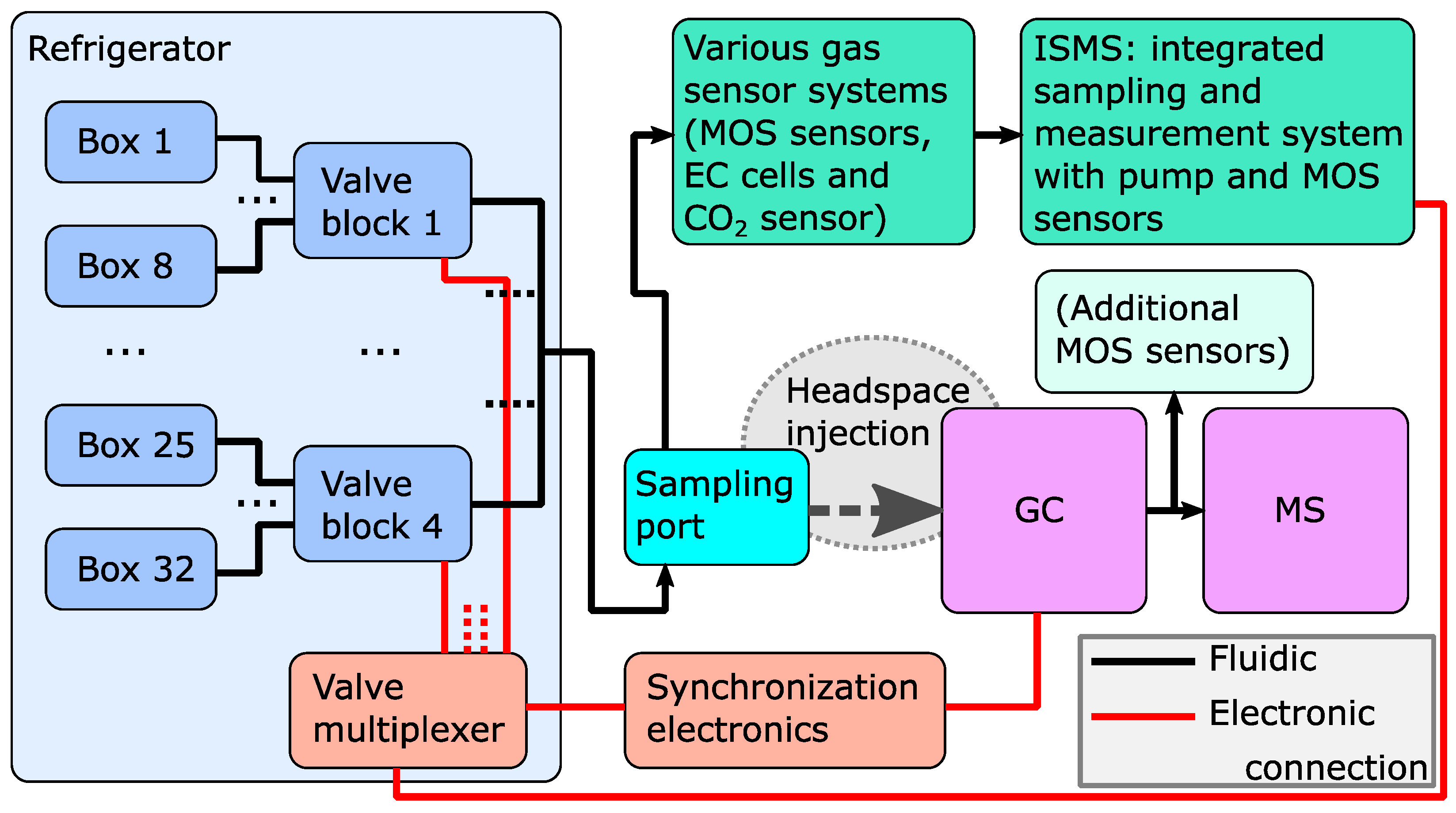
The setup is illustrated schematically in Figure 1 and consists mainly of sample containers, several gas sensor systems, and a GC-MS system; a similar setup was already used in previous measurements [29]. During the measurements, the food was stored in individual plastic food storage containers, placed in a commercial refrigerator. For the presented series of measurements, the refrigerator was turned off, and the temperature was controlled by the air conditioning of the lab, leading to a temperature of approx. 23.5 °C (±0.5 °C) within the refrigerator, also monitored by sensors for temperature and relative humidity (SHT35 from Sensirion, details see below) at three positions in the refrigerator. The volume of the food containers was approx. 1.1 L. On one side, the containers are connected to one of four valve blocks via tubes. The valves of the valve blocks allow the selective sampling of one or more containers, i.e., the food headspace, by a pump. On the other side, the containers are equipped with a check valve, allowing the inflow of air from the refrigerator to compensate for the slightly reduced pressure during sampling; for a defined background and to avoid crosstalk between samples, the refrigerator is flushed with dry, clean zero air.

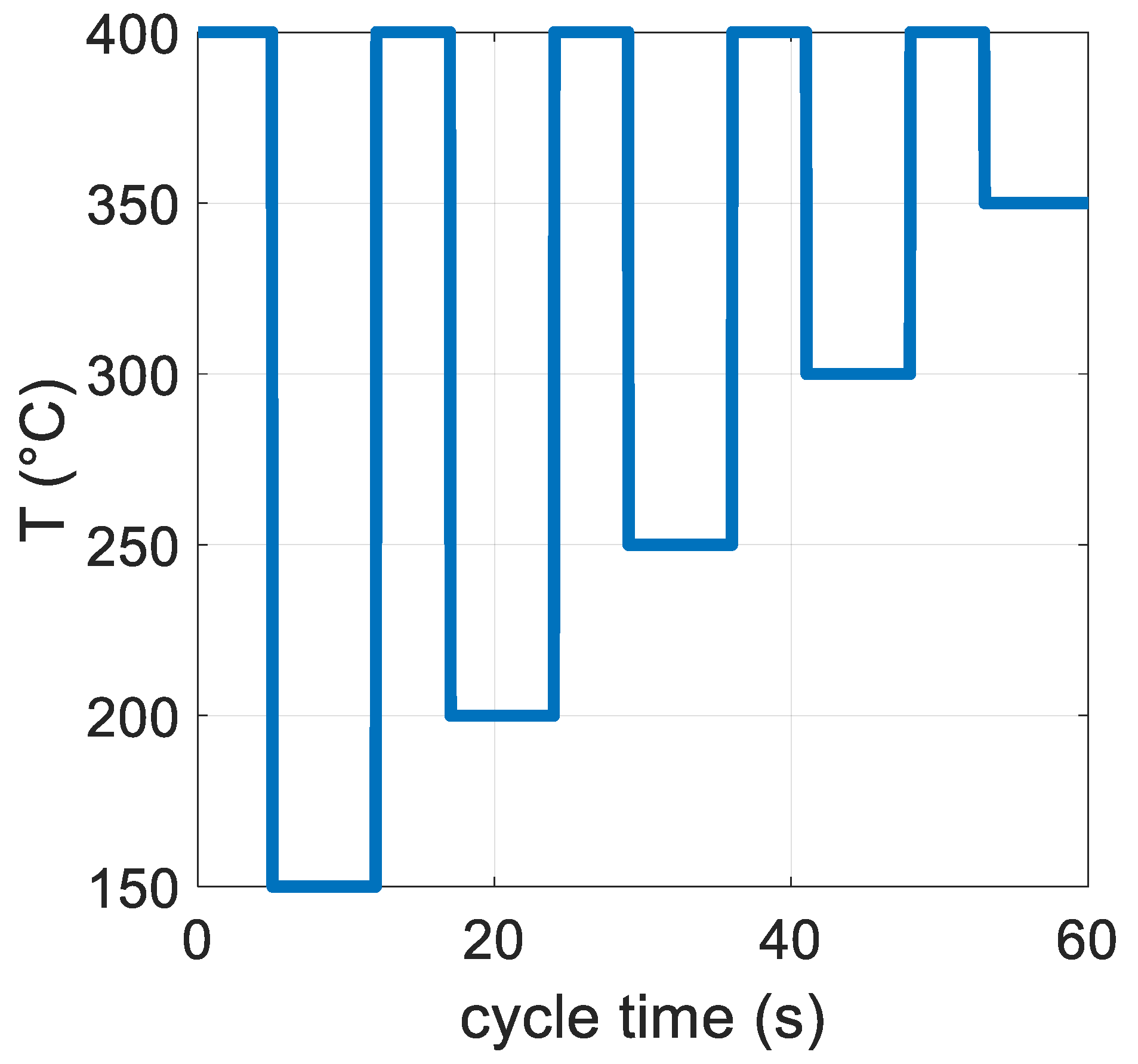
The valves and the pump are controlled by an integrated sampling and measurement system (ISMS, developmental version of the OdorCheckerSpot, OCS, 3S Technologies GmbH, Saarbrücken, Germany), also integrating several gas sensors. Further sensor systems, most of them developed in-house [30] or by 3S Technologies (developmental version of the EnvironmentalCheckerOutdoor, ECO), measure the sampled air before the flow reaches the ISMS. Most of these gas sensors are MOS gas sensors and use temperature-cycled operation with cycle durations of 30 or 60 s. The default temperature cycle of the sensors discussed within this article is a 60 s cycle, consisting of five high temperature phases at 400 °C, each 5 s long, followed by low temperature phases at 150, 200, 250, 300, 350 °C with a duration of 7 s each (cf. Figure A1); for one sensor (ZMOD4450 from Renesas, details see below), all temperatures are reduced by 100 °C based on the experience gained in previous measurements.

The following sensors are included in the sensor systems used and are discussed in this paper:

• SGP30 (digital MOS sensor with four sensing layers on one hotplate, Sensirion AG, Stäfa, Switzerland).
• ZMOD4450 (digital MOS sensor, Renesas Electronics Corporation, Tokyo, Japan).
• BME688 (digital MOS sensor, Bosch Sensortec GmbH, Reutlingen, Germany).
• Two electrochemical (EC) sensors: B-series EC cells for hydrogen sulfide and ammonia (H2S-B4 and NH3-B1, respectively, both from Alphasense Ltd., Essex, UK); these sensors are operated using an ADuCM355QSPZ evaluation board (Analog Devices Inc., Wilmington, MA, USA).
• SCD41 (photoacoustic carbon dioxide (CO₂) sensor, Sensirion).
• SHT35 (temperature and humidity sensor, Sensirion): used to monitor temperature/humidity at three positions in the refrigerator as well as in the sample flow.

A list of all sensors included in the sensor systems used can be found in Appendix A. The assignment of the sensors to the sensor systems as well as the temperature cycles used are summarized in

Table A1. Sensor systems, sensors, and temperature cycles used.

Sensor System	Sensor	Temperature Cycle
Lab electronics [30]	SGP30 (4 sensing layers)	Default, see Figure A1
	ZMOD4450	Like default, but each step 100 °C lower
	BME688	Default, see Figure A1
	SCD41	-
	SHT35	-
Lab electronics [30], MOS sensors as GC detectors	2× SGP30 (4 sensing layers)	Constant temperature 200 and 300 °C, respectively
	ZMOD4450	Constant temperature 300 °C
	BME688	Constant temperature 300 °C
Lab electronics [30], analog MOS sensors as GC detectors	2× AS-MLV-P2	Constant temperature 300 °C
Lab electronics [30], refrigerator temperature	3× SHT35	-
OCS (3S Technologies)	2× UST MOS sensors (customer specific)	60 s cycle (confidential)
ECO (3S Technologies)	2× UST MOS sensors (customer specific)	30 s cycle (confidential)
ADuCM355QSPZ	H2S-B4	-
	NH3-B1	-

in Appendix A. The default temperature cycle is depicted in Figure A1 in Appendix A.

Additionally, a GC-MS system (GC: Trace 1300, Thermo Fisher Scientific Inc., Waltham, MA, USA; column: TraceGOLD TG-624, Thermo Fisher Scientific; length 60 m, ID 0.25 mm, film thickness 1.4 µm; flow: 2 mL/min; MS: ISQ 7000, Thermo Fisher Scientific; electronic ionization (EI); mass scan range: m/z 15–300) is used to analyze the composition of the sample flow. The headspace sample can be drawn from a so-called sampling port, a block made of aluminum and polytetrafluoroethylene (PTFE) with a septum, using an autosampler (TriPlus RSH, Thermo Fisher Scientific), and a robotic sampling system equipped with a gas-tight syringe (365H2141, Thermo Fisher Scientific; volume: 100 µL). A split/splitless injector is used, and set to splitless injection (20 s, then 25:1 split ratio). As additional detectors, several MOS gas sensors are placed downstream of the GC column parallel to the MS [31]. These gas sensors are operated at a constant temperature and with additional clean (zero) air as make-up gas. The split ratio between the MS and these additional gas sensors is approx. 1:1. This approach is used to determine which sensors react to which components of the sample gas mixture [32]; this is only briefly discussed in this article.

To ensure reliable synchronization between the valve operation, the GC-MS sampling, and the sensor data, synchronization electronics were implemented based on a microcontroller. Each measurement (see next section) is triggered by the ISMS, which is programmed to follow a measurement schedule (including the valves to be opened, opening durations, and the pump flow). To synchronize the GC sampling with the valve operation, the voltage of an LED which indicates the state of the standby valve (see below) is read by an analog input of the microcontroller. When a new measurement is recognized by the electronics (i.e., the standby valve LED is turned off), the “GC ready” signal is forwarded to the autosampler, which only then starts the next sampling. In this way, the repeatability of the timing between valve operation and GC sampling and injection is in the order of a second. Moreover, the information about the valve operation as well as the GC injection is recorded as digital signals (high/low) in parallel with the sensor signals to obtain a timing reference for the data evaluation.

2.2. Measurement Procedure

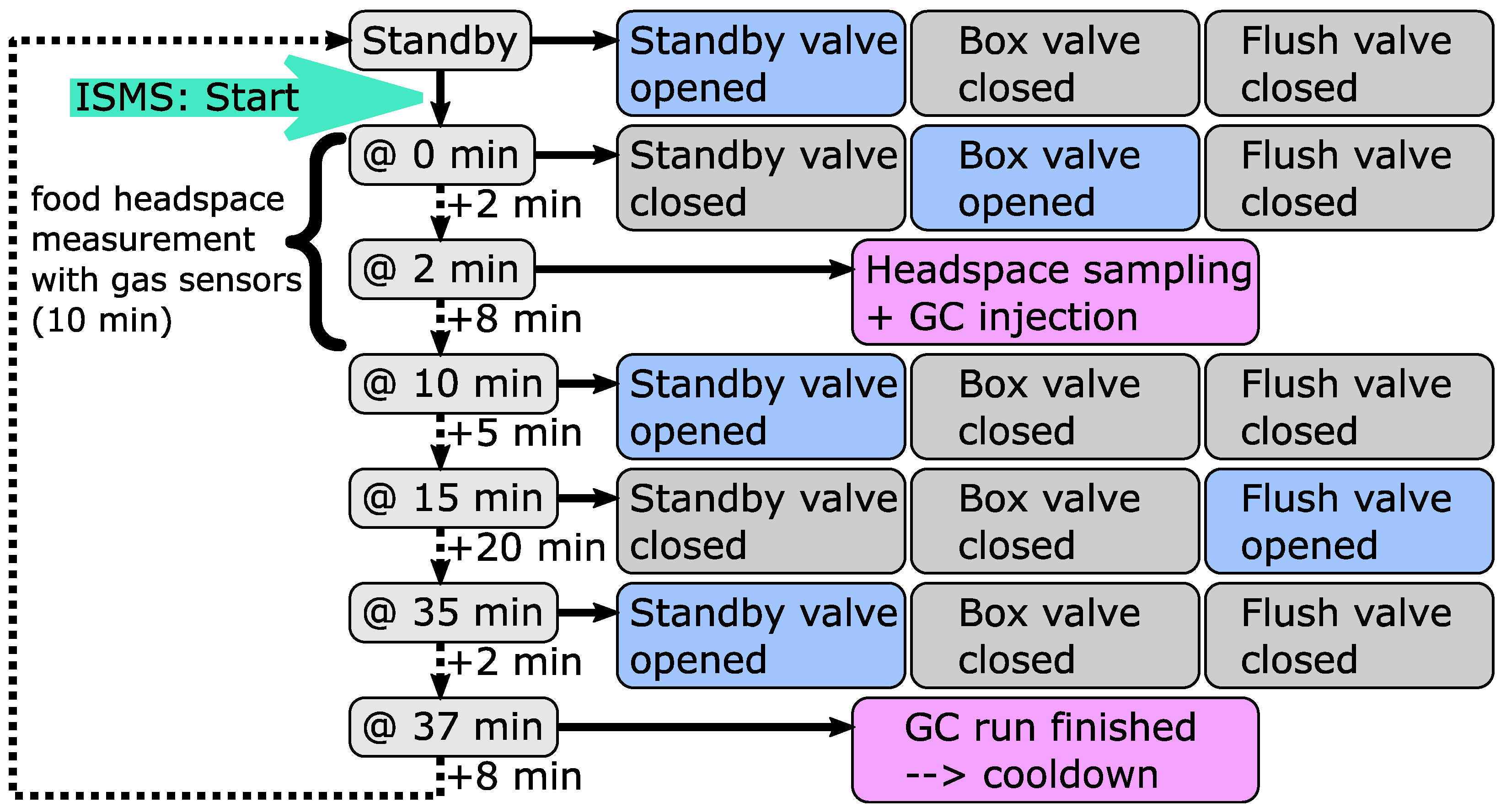
Every food container was analyzed automatically once every day. The measurement procedure is summarized schematically in Figure 2. During standby, a valve connected to the background air of the refrigerator is opened; accordingly, zero air is led through the whole setup between the measurements. A measurement is triggered according to a schedule programmed in the ISMS and starts with closing the standby valve and opening the valve of one food container. As a result, the food headspace is extracted from the container and led to the GC sampling port as well as to the various sensor systems; the pump flow is set to approx. 200 mL/min; the dead volume of the tubing system between a food container and the last sensor system is approx. 20 mL. The GC sample is taken approx. 2 min after the valve operation. As determined during optimization of the setup and the measurement procedure, the concentration of the container headspace at the position of the sampling port and the sensor systems increases during the first half minute after the valve operation due to the dead volume and diffusion effects, and it decreases slowly afterward due to dilution of the container headspace by the inflow of clean air through the check valve. The slightly delayed time of the GC sampling was chosen to allow sampling at rather stable concentrations, i.e., not at the time of its steepest decrease, and to allow flushing of the syringe several times with the sample flow before actual sampling. The total duration of the opening of the valve of one container is 10 min. Afterward, the standby valve is opened again for 5 min so that zero air is led through the setup. Then, a valve of the previously used valve block, connected to an empty container, is opened to flush the valve block and sampling tube with clean air to reduce carryover effects; this “flush valve” is opened for 20 min. Finally, the standby valve is opened for the rest of the measurement. To determine the background signal and possible residual carryover effects, an empty container is sampled and analyzed between the measurements of actual food samples; note that during these measurements, the flush valve is already opened at the start (@ 0 min) and is kept open for 35 min, i.e., the step “box valve opened” and the intermediate step “standby valve opened” are skipped. The total measurement duration is 45 min due to the GC measurement requiring 35 min after a 2 min delay plus a further 8 min for cooldown and a time buffer; thus, theoretically, up to 32 samples could be measured every day with the GC run used, but due to the flush/background measurements and a time buffer (e.g., for documentation and human assessment, see Section 2.4), 15 actual food samples are the practical daily limit. During the GC run, a temperature program is used (11 min at 40 °C, ramp with a rate of 10 °C/min up to 230 °C, 5 min hold time).

2.3. Investigated Food

In the main measurements, four containers were prepared with oranges, using three different sources and varieties (one variety from conventional agriculture, two varieties from organic agriculture), and of one of the organic varieties, two containers were prepared to investigate repeatability (from one container to another container of the same fruit from the same source/variety) and transferability (between different sources/varieties). The total measurement duration was 20 to 23 days, depending on the fruit deterioration progress; the time count of the measurement starts at 0. Note that on the last declared measurement day, only the last human assessment was performed, the last measurements using the sensor systems and GC-MS were started the day before and are assigned accordingly. In some cases, samples were intentionally damaged during the series of measurements by dropping or cutting, as damaged fruits might be an interesting target in addition to ripeness or spoilage. Details about the oranges are summarized in

Table 1. Details of the oranges used in the main measurements. Fruits marked with a star (*) were damaged by dropping at least once during the measurements.

Time Range	Fruit	Type/Variety	Agriculture	Amount	Weight
days 0–20	orange 1	Navelina 1	conventional	1	249 g
days 0–20	orange 2	Navel, same as 4	organic	1	177 g
days 0–23	* orange 3	n.a.	organic	1	250 g
days 2–23	* orange 4	Navel, same as 2	organic	1	194 g

¹ Preserved with imazalil, pyrimethanil, shellac, polyethylene wax, and potassium sorbate.

. Details about all further fruits measured during the same series of measurements can be found in Appendix A (

Table A2. Details of further fruits used in the main measurements. Fruits marked with a star (*) were damaged by dropping at least once during the measurements.

Time Range	Fruit	Type/Variety	Agriculture	Amount	Weight
days 0–20	banana 1	n.a.	conventional	1	144 g
days 0–16	banana 2	n.a., same as 3/4	organic	1	147 g
days 0–16	banana 3	n.a., same as 2/4	organic	1	146 g
days 2–16	* banana 4	n.a., same as 2/3	organic	1	133 g
days 0–23	onion 1	yellow, same as 4	organic	1	89 g
days 0–26	onions 2	red, same as 5	organic	2	86 g
days 0–26	onions 3	shallots	organic	3	94 g
days 2–26	* onion 4	yellow, same as 1	organic	1	105 g
days 0–20	onions 5 (moldy)	red, same as 2	organic	2	48 g

).

In addition, various additional fruits (including citrus fruits such as oranges, blood oranges, and a lemon) were collected from a local retail store and measured in the last days (days 23–26). These fruits had been discarded due to mold, ripeness, damage, or exceeded storage durations and were introduced mainly to collect additional data for verifying the findings of the main measurements and for testing the statistical models based on the gas sensor data. Details on these additional citrus fruits are summarized in

Table 2. Details of the additional citrus fruits collected at a retail store.

Time Range	Fruit	Type/Variety	Agriculture	Amount	Weight
days 23–26	lemon (moldy)	n.a.	conventional	1	190 g
days 23–26	blood oranges (moldy)	Sanguinelli 1	conventional	2	153 g
days 23–26	blood oranges (ok)	Sanguinelli, same as moldy, taken from the same net	conventional	2	223 g
days 23–26	orange (moldy and damaged)	Cara Cara 2	conventional	1	169 g
days 23–26	orange (ok)	Cara Cara, same as moldy and damaged, taken from the same net	conventional	1	208 g

¹ Preserved with imazalil, shellac, and polyethylene wax. ² Preserved with imazalil, pyrimethanil, fludioxonil, shellac, and polyethylene wax.

. Details about further additionally measured fruits can be found in Appendix A (

Table A3. Details of further additional fruits collected at a local retail store.

Time Range	Fruit	Type/Variety	Agriculture	Amount	Weight
days 23–26	bananas (ok)	n.a.	organic	1	369 g
days 23–24	plums (ok)	Ruby Sun (red) + Sun Kiss (yellow)	conventional	1 + 1	115 g
days 24–26	plums (damaged)	same as above, taken from the same package	conventional	1 + 1	113 g
days 23–24	grapes (ok)	Thompson Seedless	conventional	n.a.	54 g
days 24–26	grapes (brownish spots)	same as above, taken from the same package	conventional	n.a.	59 g
days 23–26	strawberries (ok)	n.a.	organic	3	103 g
days 23–26	mushrooms (ok)	white	conventional	3	141 g

).

Additionally, an organic compound mixture was put into one of the food containers on several days during the measurements to be able to track changes within the measurement setup and to estimate the concentration of some substances. The mixture was prepared by adding 75 µL of methanol, 150 µL of ethanol, 50 µL of acetone, and 75 µL of 2-butanone to 80 mL of distilled water. Using Raoult’s law as well as Dalton’s law [33], the concentrations of the substances within the headspace at 20 °C can be estimated to be approx. 53, 33, 37, and 20 ppm, respectively.

2.4. Human Assessment

The food was evaluated by two out of three persons untrained in the sense of standardized sensory evaluation (regarding either food or odor). However, they were experienced in evaluating food conditions in several measurement campaigns. On the last measurement day (day 26), the food, i.e., the additionally collected citrus fruits, was assessed by all three persons. The food in each container was evaluated once a day regarding its edibility. To be able to differentiate between visual and olfactory changes during food aging, the appearance of the food as well as its odor—more precisely: the hedonics of the odor (which is certainly influenced by individual edibility estimations learned through everyday experiences) rather than the intensity alone—were evaluated in addition to the overall edibility. Each of these measures has a scale from 10 to 1: 10 means perfectly fresh, a pleasant odor, and a flawless appearance, 1 means completely spoiled, a strong unpleasant odor, and strong visual deterioration (e.g., mold); the threshold between edible and spoiled is therefore 5.5. Regular olfactory assessment was stopped for health reasons as soon as the fruits were moldy to a significant extent. Additionally, comments on the odor (e.g., the odor quality, in case it was very prominent) or appearance were recorded, if necessary. Also, every food was photographed daily to help track the actual condition of the food during data evaluation.

2.5. Gas Sensor Data Evaluation

The data were evaluated using machine learning to predict the desired output, e.g., the edibility quantification or classification of the fruit condition (i.e., ok, damaged, or moldy). The methods applied are described in general in the following paragraphs. In all cases, the MATLAB toolbox DAV³E was used for the whole data evaluation process [34]; DAV³E v0.2 was employed, running on MATLAB R2024b.

The raw data are, in most cases, cyclic two-dimensional data. Within the course of the measurements over time, the programmed temperature cycle of a MOS gas sensor is repeated continuously. The basic idea of the data evaluation is the interpretation of the sensor signal during the temperature cycle in terms of pattern recognition using statistical models. First, data preprocessing is performed. Based on the Sauerwald–Baur model [35], logarithmic conductance is calculated from the raw signal (sensor resistance or conductance). Then, features are extracted from the cyclic data; this corresponds to a dimensionality reduction. For this, the preprocessed signal is divided into n intervals, which are aligned to the temperature steps, and the mean value and slope of each interval are calculated; in the case of the default temperature cycle, the intervals are evenly distributed and n equals 60, resulting in features that represent one second. Mean and slope features in intervals of the order of seconds yielded good results in previous research [36], and this is a reasonable choice given the typical temporal response dynamic of gas sensors (i.e., the features lead to a good representation of the signal shape) and the selection/design of the statistical models (see below), which can handle, for example, redundant and correlating features. Note that from the non-cyclic sensors (i.e., the EC cells and the photoacoustic CO₂ sensor), only a 60 s mean value is extracted as a feature, given their significantly higher time constants and more stable readings over this period of time. The calculated features are additionally standardized to ensure a similar weight of all sensors used in the trained model. The model training is divided into the training itself, validation, and testing. For testing, a part of the data set is ignored during training and validation, and these data are then applied to the trained model to determine how well previously unknown data are interpreted by the model; here, different subsets of the data are used for testing, see the results. Validation is performed during the training process using k-fold cross-validation (here, k = 10), to be able to tune model hyperparameters while avoiding overfitting. The folds of the validation were built based on whole groups (so-called group-based validation) to obtain meaningful validation errors; here, whole edibility ratings are excluded during training and projected for validation. Validation was repeated five times each with a new split. For quantification, partial least squares regression (PLSR) is used. For classification models, linear discriminant analysis (LDA, three dimensions) is used, combined with the k-nearest neighbors (kNNs) classifier (here, k = 5); before the LDA, principal component analysis (PCA, varying the optimal number of principal components, see the results) is performed for an additional dimensionality reduction and decorrelation of the feature space, as many raw features are highly correlated. In the case of quantification, the best model (i.e., the optimal set of hyperparameters) is determined by finding the model with an appropriately low root mean square error (RMSE) of validation without overfitting; in the case of classification, the percentage of correct classification during validation is considered accordingly. The use cases discussed, i.e., quantification of the fruit edibility as well as classification of the fruit condition regarding bruises and mold, are regarded as feasible if the errors obtained for model testing are reasonably low, indicating a sufficient representation of the target variable, i.e., the fruit edibility or condition, by the gas sensor data, including transfers to new fruit varieties, and thus showing a suppression of differences in the individual headspace composition.

3. Results

3.1. Reference Data: Human Assessment, GC-MS

During the measurements, only one orange remained “edible”, while the other oranges had gone moldy or had reduced edibility ratings due to (intended) damage. Significant events are summarized in

Table 3. Significant events during the measurements of the oranges.

Day	Orange 1	Orange 2	Orange 3	Orange 4
0	start	start	start
2				start
3	slightly moldy, only at the stem base			dropped once from 1 m, no immediate visible or odor change detectable
5	odor: alcoholic
7				dropped again; odor: fruity orange
13	(new moldy spot identified at photograph afterward)			dropped 3 times from 1.8 m
14	new mold at an additional spot			newly damaged spot darker
16		mold
18	very strong odor, alcoholic/varnish-like
20	end: very moldy	end: moldy spot, very soft/delicate	dropped 2 times from 1.8 m	cut: 7 cm long, 5 mm deep
23			end: looks ok, quite solid, damaged spot, soft	end: looks ok, cut appeared glued

. Oranges 1 and 2 turned moldy during the measurements, orange 3 was damaged by dropping once, and orange 4 was damaged by dropping several times and being cut once. However, the first mold spot of orange 1, starting on day 3, did not grow significantly, thus it is assumed that the orange was not infected completely, but only on the surface of the stem base, maybe due to the moist storage conditions. The moldy spot starting on day 14, on the other hand, grew rapidly in the following days. While the first mold at the stem base developed a bluish color, the growing mold was green. The mold found on orange 2 on day 16 also grew considerably; its color was bluish. After the first drop of orange 4, no significant effects could be identified based on appearance or odor; also, after the subsequent drop, no damage could be observed. Only after repeated dropping from a greater height did a dark spot remain in the following days. Also, the cut in orange 4 dried and appeared glued rather than leading to accelerated decay.

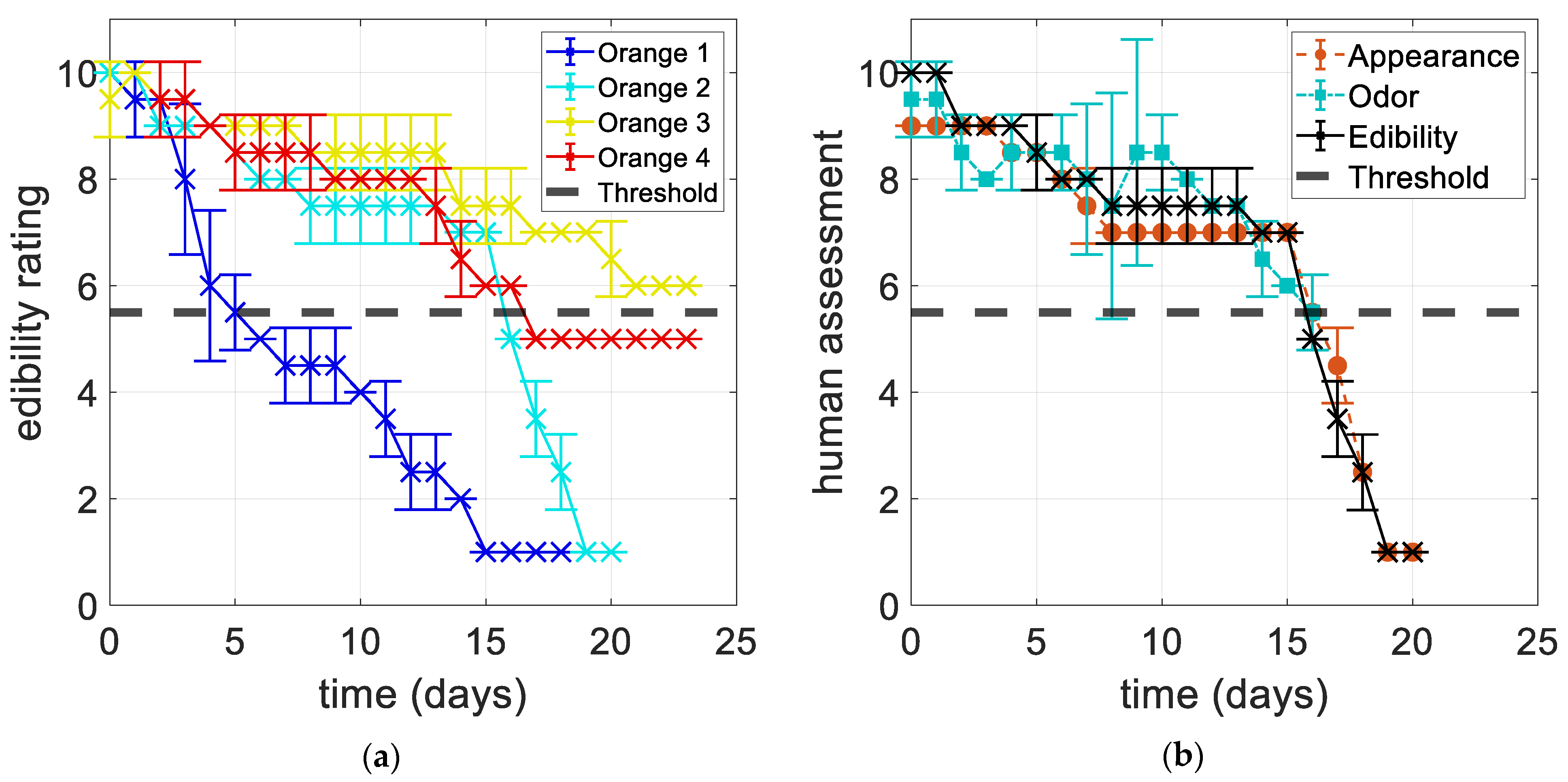
The human assessments of all four oranges, i.e., the rating of their edibility, are depicted in Figure 3a. The error bars indicate the standard deviation between the evaluating persons. The ratings of the odors and the appearances are quite similar to the overall edibility; however, as soon as an orange turned moldy, the odor was not evaluated further. As an example, Figure 3b shows all three ratings for orange 2. These ratings are actually very similar and typically differ by a maximum of one. The average standard deviations are 0.32, 0.74, and 0.35 for appearance, odor, and edibility, respectively.

Obviously, mold led to rapidly decreasing ratings of the edibility (oranges 1 and 2), but also the dark spot after dropping from an elevated height led to decreased edibility ratings (orange 4). While it is understandable that in the latter case a reduced edibility is assumed if there are visual defects, the fruit may actually have remained as edible as before; visible mold on the surface of the fruit, on the other hand, can be assumed to have already grown into the pulp, and therefore, the fruit should actually not be eaten. The first mold spot detected at the stem base of orange 1 led to a much slower decrease in the ratings compared to the mold detected on orange 2. The edibility rating of orange 3 remained above the threshold of 5.5 until the end, albeit with a slight decrease, which is similarly reflected in the ratings for odor and appearance.

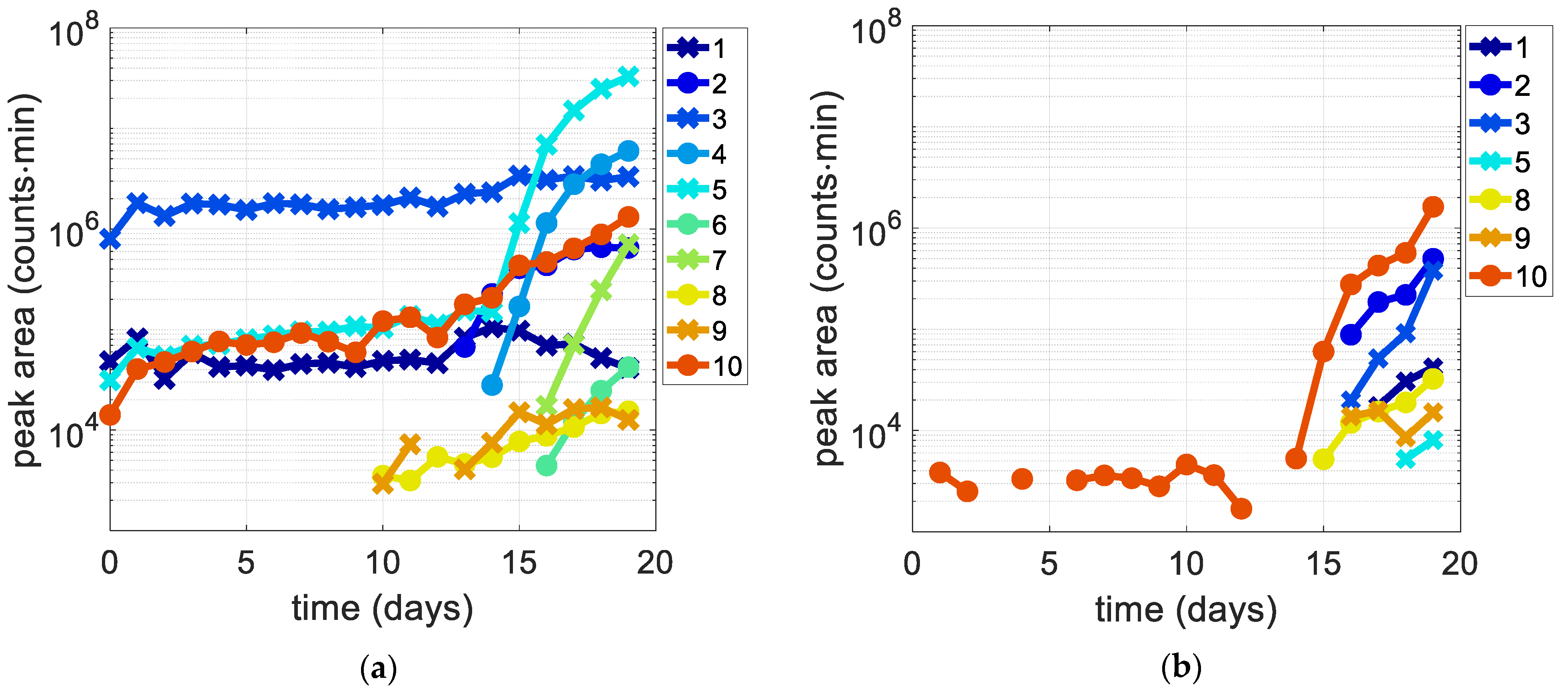
The GC-MS chromatograms were evaluated by calculating the peak area for various compounds as identified by the NIST library (NIST 17) [37]. While most substances were integrated in a channel with a broad mass range (m/z 32.5–300, which excludes background components such as nitrogen, oxygen, and water), carbon dioxide was integrated in a separate channel (m/z 43.5–44.5), and methanol was integrated using the total ion current (TIC, m/z 15–300). Empty containers (measured before and during the measurements) showed no significant background peaks (besides typical air components including carbon dioxide and water). The development of the peak area of several substances identified in the headspace of oranges 1 and 2 over the course of the measurements is depicted in Figure 4. Oranges 3 and 4 mainly emitted limonene after being strongly damaged, i.e., dropped from a great height (orange 4 on day 13 and orange 3 on day 20) and after being cut (orange 4 on day 20), with decreasing peak areas over time; note that no limonene was found after the first two times orange 4 was dropped from a lower height (days 3 and 7).

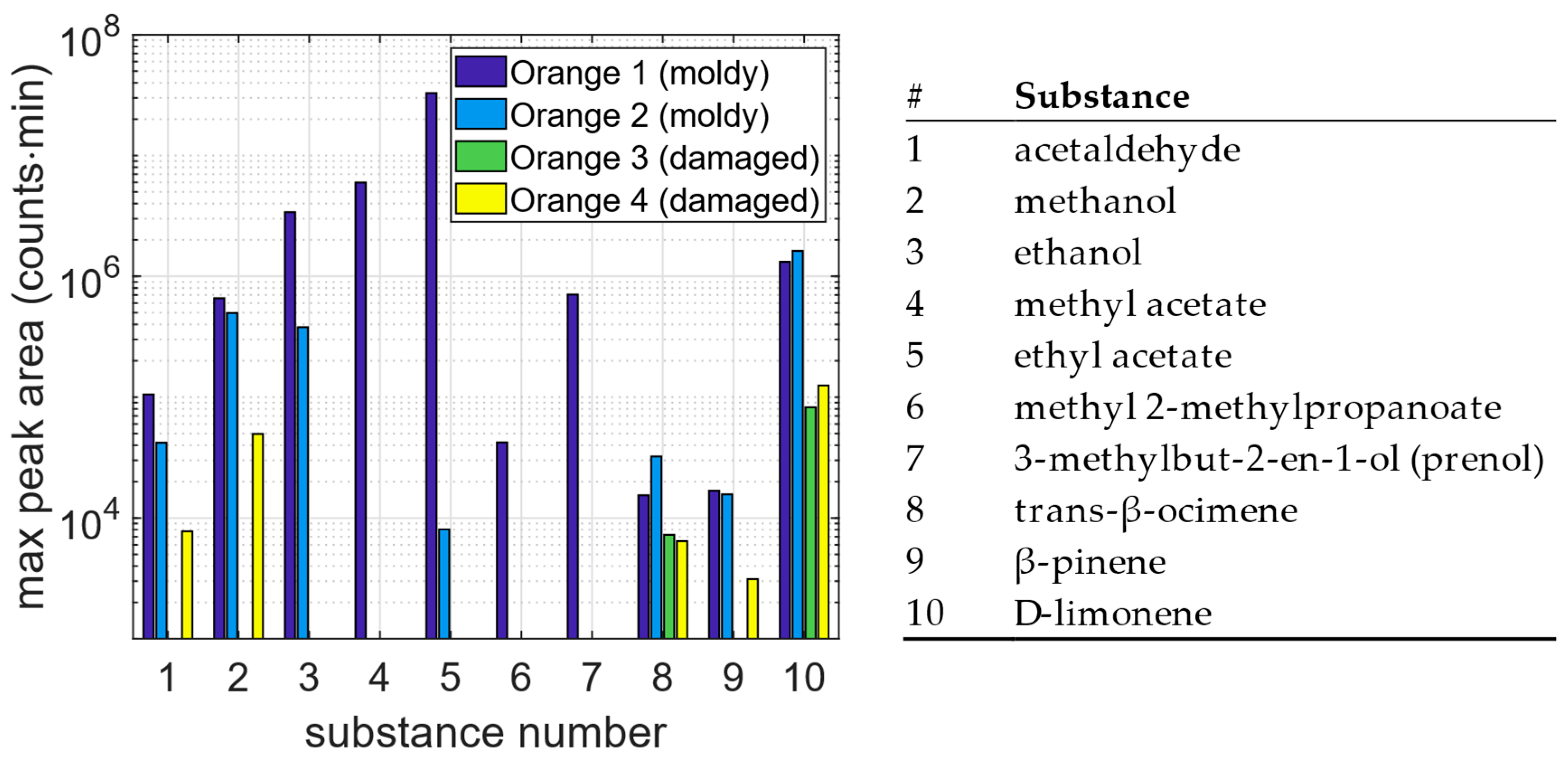
The most significant substances identified in the chromatograms and their trends are summarized in

Table 4. Substances identified by GC-MS and days of their appearance, including the peak area development: constant sample baseline (c), new (n), increasing (i), decreasing (d). Entries marked with a star (*) are the most prominent developments.

		Days of Appearance and Development
#	Substance	Orange 1	Orange 2	Orange 3	Orange 4
1	acetaldehyde	~c: 0–19 (max: 14)	ni: 17–19		(n: 13)
2	methanol	ni: 13–19	* ni: 16–19		(n: 15, 19, 20)
3	ethanol	c: 0–19	* ni: 16–19
4	methyl acetate	* ni: 14–19
5	ethyl acetate	~c: 0–14, * i: 15–19	n: 18–19
6	methyl 2-methylpropanoate	ni: 16–19
7	3-methylbut-2-en-1-ol (prenol)	* ni: 16–19
8	trans-β-ocimene	ni: 10–19	ni: 15–19	n: 20	n: 13, 14, 16
9	β-pinene	ni: 10–19	n: 16–19		n: 13
10	D-limonene	~c: 0–14, i: 15–19	c: 1–12 (gaps), * i: (14/)15–19	c: 3–6, * nd: 20–22	* nd: 13–19, * d: 20–22

. The maximum values of the same substances are visualized in the bar chart in Figure 5. There were several further substances identified, especially for orange 1, either from the start of the measurements (e.g., 2-pentanone, decreasing from the beginning; ethyl propanoate and ethyl butanoate, both slightly increasing from day 15 on) or emerging during severe mold (e.g., methyl butanoate and ethyl 2-methylpropanoate, both starting on day 14).

Combining the results from human assessment and GC-MS data, several conclusions can be drawn:

• Limonene is the only substance (besides water, carbon dioxide, etc.) that could be found in the baseline emission of several oranges (1, 2, and 3; it was found in the headspace of orange 4 only after dropping from elevated height). It can be assumed that limonene is a key substance contributing to the (in some cases only slight) odor of intact and fresh oranges.
• For orange 1, the baseline emission consisted of more substances with higher concentrations. In addition to limonene, several alcohols (most prominently ethanol), esters (ethyl acetate, ethyl butanoate), and acetaldehyde were detected. It is worth noting that this orange was the only orange in the presented measurements (apart from the additional fruits used for testing) resulting from conventional agriculture and, according to the label, it had been preserved (with imazalil and pyrimethanil) and waxed (with shellac, polyethylene wax, and potassium sorbate). It was also the only orange for which an alcoholic odor was reported before severe mold growth was detected.
• The oranges damaged by dropping or cutting (oranges 3 and 4) emitted mostly limonene (and other terpenes) with concentrations decreasing over the following days. However, the concentrations emitted after dropping from low heights, i.e., after causing only slight damage, were not high enough in all cases (or decreased too fast) to be measured, as the damages caused to orange 4 on days 3 and 7 could not be observed with GC-MS, although a typical orange odor was detected by human assessment at least for day 7. Only the (more severe) damages caused on days 13 and 20 resulted in significant terpene emissions.
• Mold, developed on oranges 1 and 2, led to high emissions of alcohols, esters, and terpenes; however, the specific compositions were different in these cases. While increasing peak areas of ethyl acetate, methyl acetate, and prenol were dominant during mold development on orange 1, orange 2 primarily showed emissions of limonene, methanol, and ethanol. Peak areas of methanol and limonene were also increasing for orange 1, but they were not as dominant as those for orange 2, and ethanol increased only slightly for orange 1. Conversely, the dominant species of orange 1 were observed with smaller peak areas (ethyl acetate, methyl acetate) or not found at all (prenol) for orange 2. These differences might originate from different mold species, as indicated by the different colors. The odor of the very moldy orange 1 was described as alcoholic and varnish-like, which matches the increased concentrations of, for example, ethyl and methyl acetate, which are commonly used as solvents.
• When comparing the timing of the mold events, the GC-MS measurements show new substances or increasing peak areas on the same day or even one day earlier than when the human assessments suggest the starting of spoilage. For example, significantly increasing limonene peak areas were detected for orange 2 from day 15 onward, and ocimene was additionally detected starting on that day, while mold was only observed on day 16. Similarly, severe mold on orange 1 was reported on day 14, while methanol was already detected on day 13 (methyl acetate emerged on day 14, and ethyl acetate increased from day 15 on). Note that the new mold spot of orange 1 could already be identified in the photographs on day 13, but it was not recognized as an early mark of mold by the human evaluators. Furthermore, the odor assessment of orange 2 dropped below the assessment of the appearance and the overall edibility a day before mold was visually identified, indicating that some degradation-related change might already have been perceived by the nose, but not yet by the eye, consistent with the GC-MS results that show already increasing terpene concentrations at that time.

In summary, several substances could be identified that are correlated to the damaged or moldy oranges in the presented measurements. While limonene could be found in both cases (and also in the headspace of intact fruits), additional components such as alcohols and esters were increasingly emitted by moldy oranges, matching the odors identified during human assessment. The differences between oranges, both in the baseline emission and the substances found for the investigated events (especially mold), indicate that there is not one unique substance or substance mixture that is observed for all oranges or all types of molds. Note that, in general, the sample size of four oranges is too limited to draw general conclusions.

The additional fruits collected at a local retail store were measured similarly, but only for three days (again, the human assessments were performed for one additional day compared to the measurements with the sensor systems and the GC-MS). For most of the fruits investigated, flawless samples could be taken from the same net or package in which the damaged or moldy samples were found. In these cases, both flawless and moldy fruits were measured, allowing a comparison of these two conditions despite the short measurement duration.

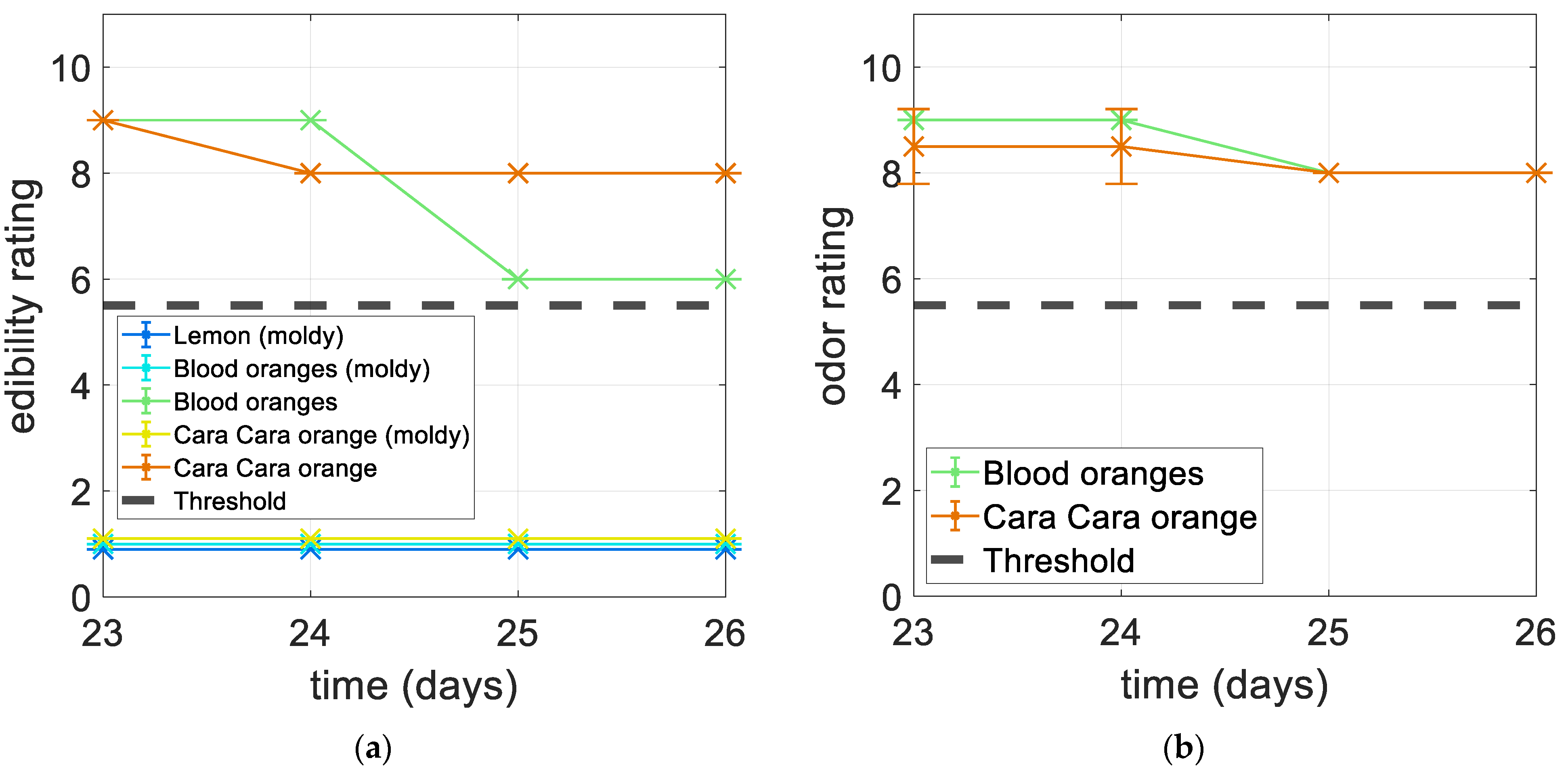
The human assessment results are shown in Figure 6. During the three-day measurements, the edibility of most fruits did not change significantly. In the case of already moldy fruits, the ratings could not decrease further as they had already reached the minimum at the very start. However, further mold growth could be observed in all cases (lemon: green mold; blood oranges: blue mold, with a smaller part green; Cara Cara orange: mostly white mold with a small green area). However, a small spot of bluish mold was found on one of the two initially flawless blood oranges on the last day, which led to a decrease in edibility, while the odor assessment did not change significantly. Also, a yellowish liquid leaked from the moldy and quite squishy Cara Cara orange after the first day, the odor was described as strong and alcoholic. In general, the odor of the moldy citrus fruits was described as alcoholic, sour, and sometimes fruity (blood oranges and Cara Cara orange); in comparison, the odor of the flawless (blood) oranges was described as fruity, and orange-like.

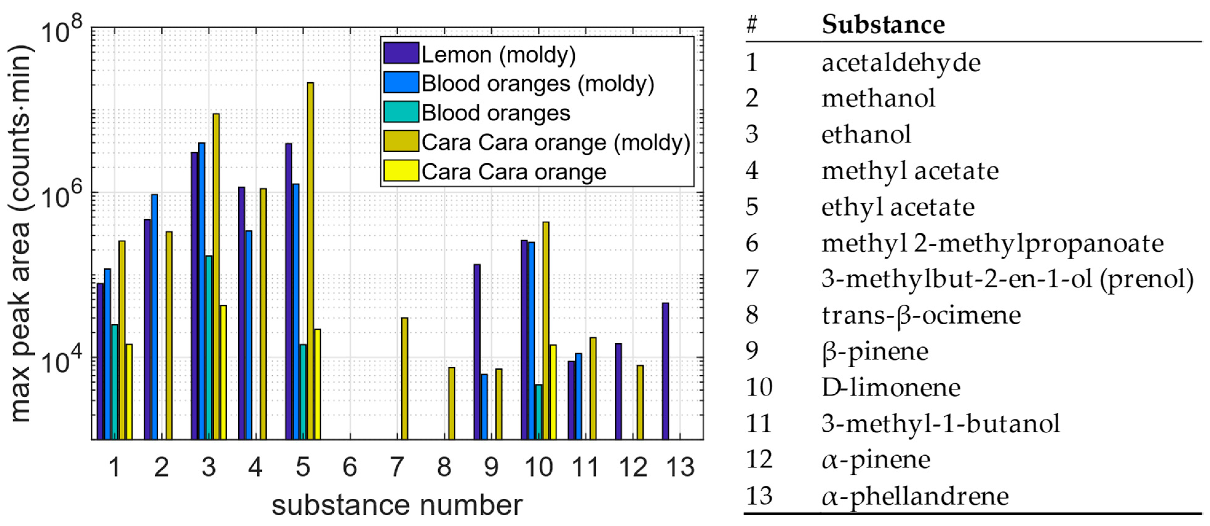
The results of the GC-MS measurements, i.e., maximum peak area of the most significant substances, are depicted in Figure 7. Comparing flawless and spoiled fruits, the findings of the main measurements presented above are confirmed: mold led to increased emissions of ethyl acetate, ethanol, limonene, and acetaldehyde (except for orange 1, for which no clear increase in acetaldehyde was observed), and the emission of additional substances such as methanol, methyl acetate, and β-pinene. The moldy Cara Cara orange additionally emitted prenol, which was also very prominent for the severe mold of orange 1, and ocimene, which was also found for the previously measured moldy or damaged fruits. Three additional substances are included in Figure 7: 3-methyl-1-butanol (which was also observed for orange 1 in the main measurements, but was less prominent), α-pinene, and α-phellandrene; the latter was only observed for the moldy lemon, which also showed higher levels of β-pinene compared to the moldy oranges.

Several of the substances identified for moldy fruits were also found in the headspace of flawless fruits, namely ethanol, acetaldehyde, ethyl acetate, and limonene. Ethyl butanoate could again be identified for all four additional oranges, but in very small concentrations. These are the same substances found for orange 1 in the main measurements even before the first severe mold growth was observed. Note that orange 1 and the initially flawless additional oranges had two aspects in common: they had been preserved with a fungicide coating, and they either had contact with infected fruits (as the additional fruits were taken from nets in which moldy fruits were also found) or, in the case of orange 1 and the blood oranges, developed slight mold themselves. Thus, possible reasons for the additional substances observed for these three oranges but not observed for the other three organic, non-preserved oranges, even when they were flawless, might be emissions caused by the preservation, or from subliminal infection. Note that no altered emissions by preservation coatings have been reported in the literature.

Even though one of the two blood oranges had developed a small spot of mold on the last day, no significant change in the headspace composition was observed by GC-MS, matching the result of the odor assessment. Also, the peak areas of the already moldy fruits were quite stable during the three-day measurements; the most prominent changes were observed for the moldy lemon (limonene increased by a factor of approx. 6 while methyl acetate and ethyl acetate decreased by a factor of more than 10) and the moldy blood oranges (in contrast, methyl acetate and ethyl acetate increased by a factor of approx. 5).

A quantitative estimation of the observed concentrations of methanol and ethanol measured by GC-MS can be obtained as a solution with methanol, ethanol, acetone, and butanone was prepared and put into one of the food containers, cf. Section 2.3. The estimated concentrations of the substances within the headspace (53, 33, 37, and 20 ppm, respectively) are maximum values, assuming that 1 mL of the solution can saturate the headspace of one food container with a volume of 1 L. This is only just the case for the ketones (with approx. double the required amount of substance); moreover, a rather steep decrease of the peak areas after the day the solution was dropped into the food container was observed, supporting the estimation. For the alcohols, which are more important for the discussed fruits, the ratio between the expected amount of substance in the headspace and the available amount of substance in the solution is more appropriate (approx. 5–8); this estimation is supported by a much less steep decrease of the peak areas in the subsequent days. Moreover, a linear correlation between headspace concentration and peak area is assumed. Note that the estimated values are only valid for the setup used, as storage volume, air exchange rate, and storage time all strongly impact the effective concentrations. All estimated concentrations are summarized in

Table 5. Estimated methanol and ethanol concentrations of the fruits tested in selected conditions. The ranges for moldy fruits indicate values for the first day mold was observed and for subsequent development. The values of (moldy) oranges for which an alcoholic odor was reported are marked with a star (*).

	Concentrations in ppm
	Methanol		Ethanol
Fruit	Ok	Moldy	Ok	Moldy
orange 1	none	20–200 *	220	415 *
orange 2	none	25–155	none	2–45
lemon	n.a.	140 *	n.a.	130–390 *
blood oranges	none	290 *	14–18	(22–/) 1 260–520 *
Cara Cara orange(s)	none	100 *	5	415–1150 *

¹ Initially “OK” blood oranges of which one developed a small spot of mold on the last day.

.

In summary, regarding the substances a concentration can be estimated for, mold was characterized by a headspace concentration in a confined storage volume of at least several tens and up to several hundred ppm of methanol, while for the flawless fruits no methanol was observed in the headspace (i.e., concentrations (far) below 10 ppm). Ethanol, on the other hand, could also be found in the headspace of flawless fruits with concentrations up to 20 ppm; orange 1 already showed concentrations of a few hundred ppm even before (severe) mold. Mold led to a very broad range of ethanol concentrations between a few ppm and more than 1000 ppm, and concentrations for slight and severe mold differed significantly depending on the fruit. Therefore, ethanol appears to be a less suitable marker substance for mold compared to methanol.

Further analysis of the observed alcohol concentrations and parallel odor assessments indicate that at least a few hundred ppm of ethanol and/or methanol in the confined storage volume were required before the odor was described as alcoholic. The odor of the Cara Cara orange with more than 1000 ppm ethanol and approx. 100 ppm methanol was described as strongly alcoholic. Ethanol concentrations up to approx. 20 ppm remained undetected.

It can be expected that several further substances identified with GC-MS contribute to the distinct odor of both flawless and moldy or damaged fruits, e.g., limonene, methyl acetate, and ethyl acetate. To allow an estimation of the concentrations of these and further compounds, a calibration with a mixture of these substances with known concentrations would be required to determine the respective response factors. However, their concentrations are expected to be in a comparable range as methanol and ethanol (i.e., a medium to high ppm range) when they are among the relevant odor compounds. Note that the actual concentrations during a human assessment will be different as opening the food containers will lead to swift dilution in the room.

3.2. Sensor Data Evaluation

In the following, only a subset of the sensors used (the digital sensors operated with the sensor systems developed at our lab and one of the EC cells) is discussed for simplicity. Also, the results should not be seen as a detailed benchmarking of the listed sensors, but they should provide an insight into the spectrum of possible evaluation directions, including common challenges and differences in the ability to fulfill certain tasks in the given application example, i.e., the assessment of the condition of the oranges.

In general, data evaluation starts with the raw data, e.g., the pattern of the MOS gas sensors operated with TCO can be compared for different fruits, fruit conditions, etc. In fact, the events discussed regarding oranges, i.e., mold or damage, led to distinct changes in the cyclic sensor conductance of several sensors, and differences in the sensitivity towards these events can be identified between the sensors used. For example, on the one hand, damaged oranges led to a much larger change in the signal pattern for the ZMOD4450 and the BME688 than for the SGP30; this could be interpreted as a much smaller sensitivity of the SGP30 towards limonene. On the other hand, the SGP30 has a clearer change in the sensor signal during the mold development of oranges than the ZMOD4450, while the BME688 even exceeds the upper limit of the measurement range in some parts of the temperature cycle for very spoiled oranges. However, several other changes in the signal that are not quite covered by the events discussed and identified by human assessment and/or the GC-MS system can be observed. For some sensors, the pattern slightly changes/shifts throughout the series of measurements, which might be attributed to sensor drift, the aging of the fruits (without being able to identify a substance or odor that causes these changes), or, in some cases, a change in the composition of the background air in the refrigerator. The latter is not desirable, but a certain influence of very spoiled bananas (that were measured during the same series of measurements) on the “baseline” of some gas sensors was found; however, no corresponding substances were identified by GC-MS, thus either the concentrations are below the limit of detection of the GC-MS system or the changes are caused by a substance/substances not detectable with the GC-MS system, such as hydrogen. On the other hand, the undesired change in the background composition can be seen as an unintended opportunity to train models that suppress these changes.

The sensor data were evaluated as described in Section 2.5, i.e., features were extracted from the preprocessed sensor data prior to model training. To assess the applicability of gas sensors to the evaluation of the condition of oranges, both quantification models (PLSR) and classification models (PCA + LDA + kNN classifier) were developed. The target of the quantification model was the edibility of the oranges obtained by the human assessments on a scale of 10 to 1, i.e., the human assessment was taken as the reference/output value for the model. The condition of the oranges, i.e., flawless, moldy, and damaged, was used as the target of the classification model. All models were trained individually for each sensor used. The dimensions of the PLSR and the PCA (the number of components, nComps, and number of principal components, nPCs, respectively) were varied, and the best value was identified by finding a low training and validation error, that is, a dimension that leads to a sufficiently trained model without overfitting.

For the quantification model, the data of the main measurements are used for training and the data of the additional fruits collected at a local retail store are used for testing. The number of unique observations, i.e., data from one fruit on one day, used for training and testing, were 83 and 12, respectively. Note that every unique observation consists of 4 samples, i.e., temperature cycles, resulting in 332 and 48 samples for training and testing, respectively. Thus, approx. 13% of the data used for this model is reserved for testing. The root mean square errors (RMSEs) of the PLSR models are summarized in

Table 6. Root mean square error (RMSE, on the scale of the edibility rating from 10 to 1) of the training, cross-validation, and testing of the PLSR and the best number of components (nComps).

		RMSE
Sensor	nComps	Training	Cross-Validation	Testing
SGP30	5	0.69	1.36	1.12
(single elements)	5–6	0.57–1.07	0.88–1.55	1.34–1.82
ZMOD4450	5	0.80	1.22	2.43
BME688	5	0.98	1.46	2.82
SCD41 (CO2)	(1)	2.26	2.64	2.94
EC: H2S-B4	(1)	1.33	1.47	2.72

. The best results, based on the overall performance (especially the testing error, i.e., the prediction of the fruits completely unknown to the model), were obtained with the SGP30. Note that this sensor actually comprises four different sensing layers [21], thus providing considerably more raw data compared to ZMOD4450 and BME688 with only one layer each. The RMSE values for models trained with only one of the four sensing layers of the SGP30 individually are summarized for comparison with the other two digital MOS sensors, i.e., having the same dimensionality of the feature space, showing slightly inferior results regarding the testing error compared to the model using all four sensing layers.

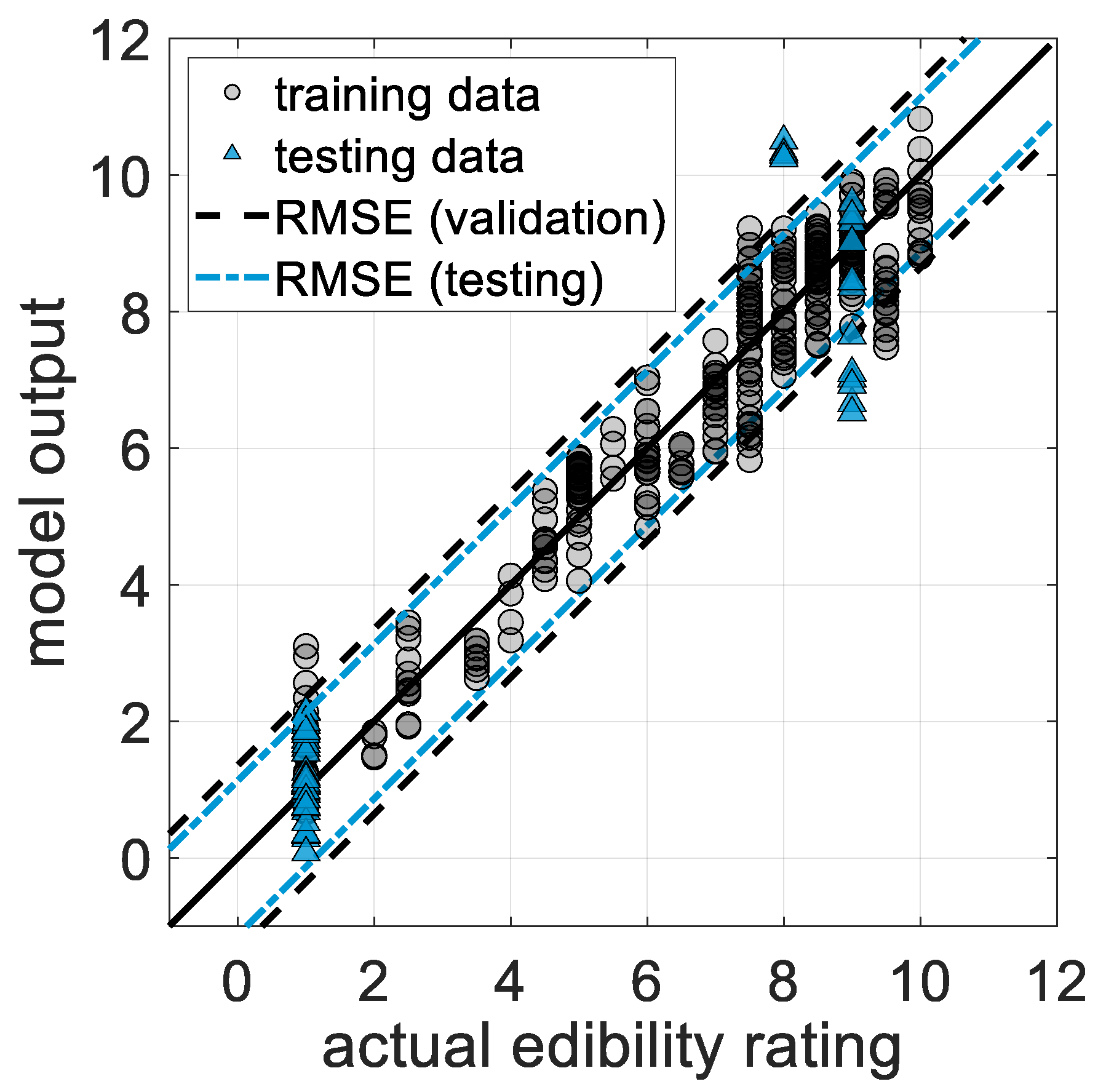
The calibration plot for the SGP30 is depicted in Figure 8. The calibration is successful, as the model can project the features to the target values, i.e., the edibility from the human assessments, with an RMSE not much larger than 1, both during validation and testing. Compared to the standard deviation of the edibility assessment of 0.35, this is significantly larger; however, given the value range of [1, 10], an RMSE of not much more than 1 is reasonable. In fact, it can be assumed that human assessment does not fully represent the fruit condition as perceived by a gas sensor; consequently, achieving a perfectly trained model is unlikely. Especially the low testing error, i.e., the good prediction of the additionally collected fruits which were either “OK” or moldy, could not necessarily be expected, as these fruits were new varieties (blood orange, Cara Cara orange) or even a completely different type of citrus fruit (lemon) not covered by the training data set. However, the models obtained with the other sensors were less successful especially in projecting the testing data, even when the validation yielded results comparable to those for the SGP30. On the other hand, this matches the observation that the SGP30 had the largest signal changes of the sensors discussed here for mold (without exceeding the measurement range), while it was less sensitive for detecting damages (i.e., limonene) than the other sensors. Both might be helpful here, as the edibility is much more affected by mold than by damage (cf. the results for the human assessment above).

The data annotation for the classification models was based on both the human assessments and, in a supporting role, the GC-MS results. Four conditions were defined as desired outputs: “OK”, “damaged: bruised”, “damaged: cut”, and “moldy”. However, only “OK” and “damaged: cut” are distinct from the other groups. For the remaining two conditions, a more or less pronounced transition is observed, thus these groups are rather heterogeneous. For the first classification model, only the data of the main measurements were considered, and only unequivocal cases were used for training, while the rest (i.e., the data between these cases) were used for testing. The number of unique observations, i.e., data from one fruit on one day, used for training and testing, were 64 and 19, respectively. Note that every unique observation consists of 4 samples, i.e., temperature cycles, resulting in 256 and 76 samples for training and testing, respectively. Thus, approx. 23% of the data used for this model is reserved for testing. Note that this leads to overestimated testing errors, as these are “in-between” cases where a correct prediction cannot be expected. “Moldy” was trained only with data from samples where the mold definitely grew in the following days; i.e., the first mold at the stem base of orange 1 was regarded as a transition case and used for testing. “Damaged: bruised” was only used for training when either the human assessment suggested increased odor after dropping or when increased peak areas of limonene, for example, were observed in the GC-MS analysis; i.e., the days after the first two times that orange 4 was dropped were used for testing, as well as the day of the first induced damage. Additionally, the days after these two damages were labeled as “OK”, as no substantial damage appeared to have been caused.

In general, a certain number of principal components is needed in the PCA to obtain a suitable representation of the data in the LDA. Too few components leads to individual “paths” of the different oranges in the LDA plot (as well as in the first three dimensions of the PCA) rather than combined clusters according to the trained groups (i.e., the conditions defined above). In most cases, 20 to 30 principal components allow a sufficiently trained model that suppresses the influence of the individual fruits and instead allows a clustering of the four conditions, but without overfitting on the training data. The optimal number of principal components and the corresponding classification errors (in percent) are summarized in

Table 7. Classification errors of training, cross-validation, and testing of the first classification model with unequivocal samples used for training and intermediate cases for testing (PCA for dimensionality reduction, LDA for class separation, kNN for final classification); nPCs gives the best number of principal components for the models.

		Classification Error (%)
Sensor	nPCs	Training	Cross-Validation	Testing
SGP30	30	1.6	6.2	30.3
(single elements)	5–20	1.6–5.1	4.6–8.7	25.0–36.8
ZMOD4450	30	1.6	10.8	23.7
BME688	15	3.5	11.2	47.4
SCD41 (CO2)	-	16.4	30.1	75.0
EC: H2S-B4	-	21.1	29.0	53.9

. The best results, based on the overall performance and especially the testing error, i.e., the prediction of the transition cases, are obtained for the ZMOD4450. The highest validation errors can be found for the “damaged” groups, as they are sometimes misclassified as the other “damaged” group.

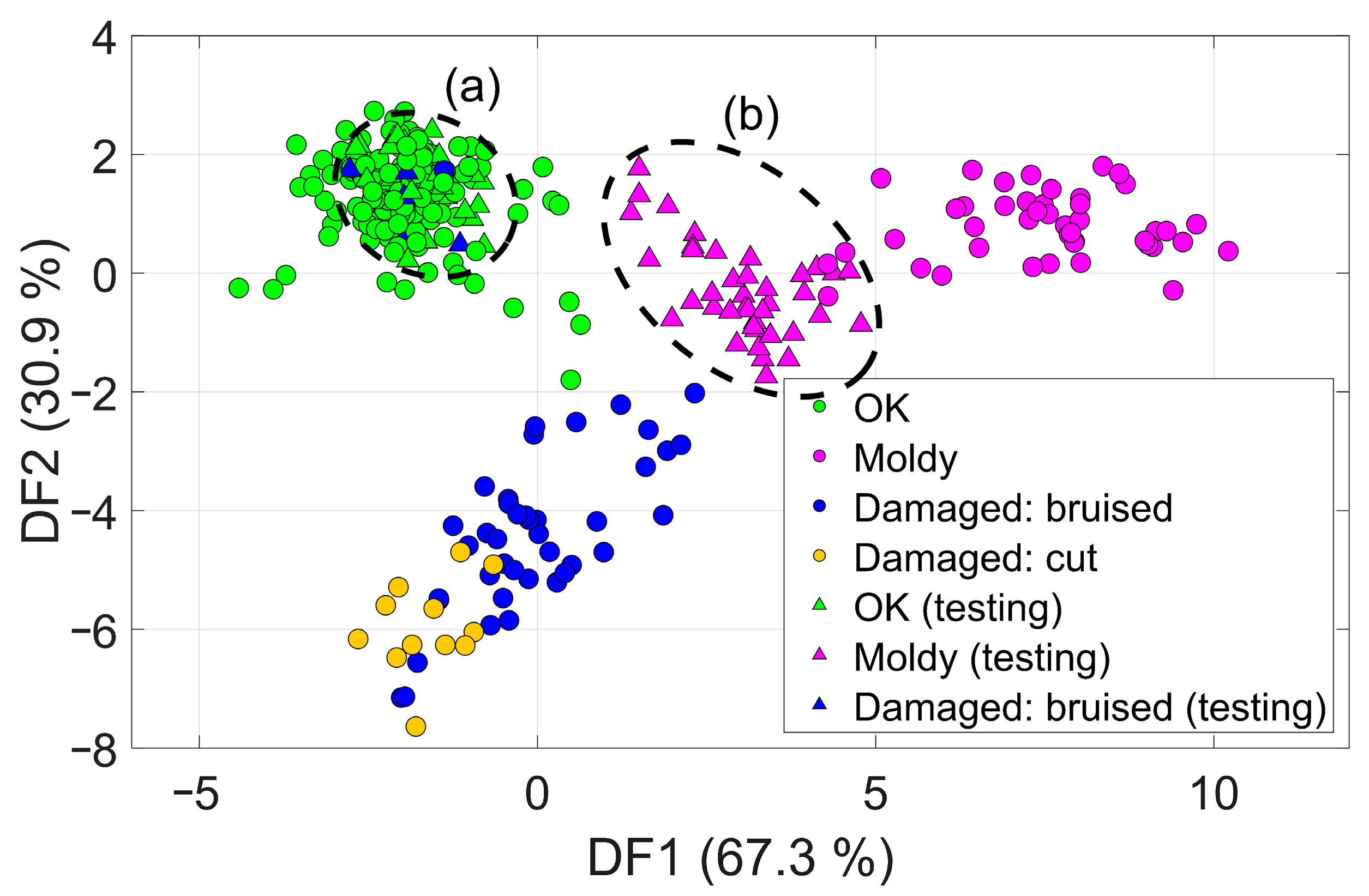
The LDA scatter plot of the ZMOD4450 is depicted in Figure 9. Several observations can be made from the LDA plot (which, if not stated otherwise, can be similarly found for the other MOS sensors discussed):

• Both the training and testing data from the day orange 4 was dropped the first two times are projected into the “OK” cluster, indicating that no damage occurred, in agreement with the human assessment and the GC-MS analysis.
• Both “damaged” cases (bruised and cut) are very close, again in agreement with the GC-MS analysis (in both cases, limonene is mainly emitted). These two groups therefore also usually have the largest validation errors.
• The transition between “OK” and “moldy” (i.e., the slight mold at the stem base of orange 1 was used for testing) is indeed projected between the “OK” cluster and the “moldy” cluster, forming a “path” between them (to varying extents for the different sensors).
• The training data points of orange 2 already trend out of the “OK” cluster towards the “damaged: bruised” cluster one day before mold was identified by the human assessment (day 15 vs. 16). This again matches the GC-MS results, where a significant increase of limonene was already observed on day 15.
• The LDA for the ZMOD4450 shows a clear separation between the group “OK” and all other groups: “moldy” is separated from “OK” and “damaged” mainly via the first discriminant function, DF1; and “damaged” is separated from “OK” and “moldy” mainly via the second discriminant function, DF2.

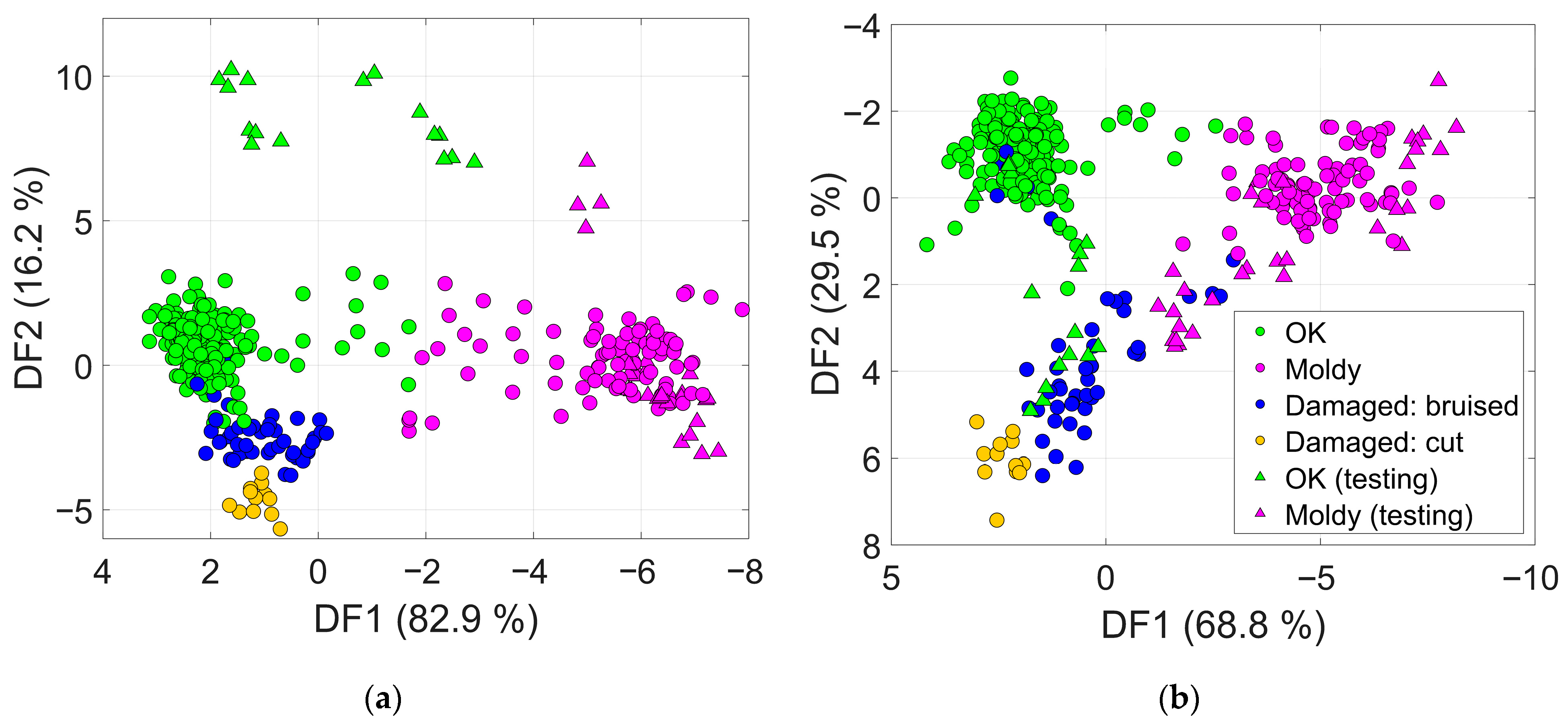
In the second step, the additional citrus fruits collected at a local retail store were used for testing of the classification model (as performed before for the regression model). In this case, the previously excluded transition cases were included in the training data set and labeled as before; i.e., orange 4 was labeled as “OK” even after the first two times it was dropped as it was apparently not substantially damaged. Only the data from the days on which this orange was dropped the first two times are labeled as “damaged: bruised”, as the typical orange odor was actually detected by human assessment at least right after the second time the orange was dropped at least, even though in none of these cases were terpenes found in the GC-MS analysis. The number of unique observations, i.e., data from one fruit on one day, used for training and testing, were 83 and 12, respectively. Note that every unique observation consists of 4 samples, i.e., temperature cycles, resulting in 332 and 48 samples for training and testing, respectively. Thus, approx. 13% of the data used for this model is reserved for testing. The results are summarized in

Table 8. Classification errors of training, cross-validation, and testing of the second classification model using all the data of the main measurements for training and the data of the additionally collected fruits for testing (PCA for dimensionality reduction, LDA for class separation, and kNN for final classification); nPCs gives the best number of principal components for the models.

		Classification Error (%)
Sensor	nPCs	Training	Cross-Validation	Testing
SGP30	15	3.3	10.5	0
(single elements)	15–20	3.6–6.3	9.8–13.8	0–20.8
ZMOD4450	30	3.0	10.5	37.5
BME688	10	2.1	14.4	8.3
SCD41 (CO2)	-	23.5	46.0	20.8
EC: H2S-B4	-	22.6	30.7	27.1

. The best model, based on overall performance (especially the testing error, i.e., the prediction of the additionally collected fruits), is again obtained for the SGP30, although in the first classification model, the ZMOD4450, performed best. For the latter, the highest validation errors can again be found for the group “damaged: bruised” (either classified as “damaged: cut” or, for the first two non-severe damages, as “OK”) and “damaged: cut” (often classified as “damaged: bruised”). For the SGP30, misclassification during cross-validation mainly occurs for “damaged: bruised” samples, which are then often classified as “OK”, as these two groups are not clearly separated. Also, some “OK” data points are classified as “damaged: bruised” or “moldy”. The latter happened for the previously discussed “transition” of orange 1 to slight mold at the stem base and is also observed for the ZMOD4450. Note that, as discussed above for the quantification model, the SGP30 comprises four sensing layers providing a higher dimensionality of the feature space; thus, the RMSE values for models trained with only one of the four sensing layers of the SGP30 are summarized for comparison, showing similar or inferior results, depending on the sensing layer.

The LDA plots for both the SGP30 and the ZMOD4450 are depicted in Figure 10. In both cases, the models trained with the whole data set of the main orange measurements are similar to the previous models in which the transition cases were used for testing, cf. Figure 9 (ZMOD4450 only). However, the projection of testing in the second model, i.e., the additional fruits collected at a local retail store (either “OK” or “moldy”), is quite different for the two sensors. The model for the SGP30 projects “OK” data with a fairly large distance from the training data, and only some data from moldy fruits lie within the trained “moldy” cluster. However, the kNN classifier correctly classifies all the data, resulting in a classification error of zero, mainly due to the matching projection in the first discriminant function. In the model for the ZMOD4450, the testing data are projected within the region of the trained clusters; however, not all of them lie within the expected groups, increasing the testing error to 37.5%. Mold is quite well projected, but some of the data points are closer to the “damaged: bruised” training data. Although the testing data of the moldy blood oranges appear to lie within the cluster of “damaged: bruised” oranges, they are in fact separated in the third dimension (third discriminant function, not depicted). Nevertheless, most of these data points are classified as “damaged: bruised” instead of “moldy”. Projection and classification of the other moldy citrus fruits (the Cara Cara orange and lemon) were, however, successful. Finally, while some of the “OK” testing data lie within the “OK” cluster, some (Cara Cara oranges) are projected into the “damaged: bruised” cluster.

Some of these observations are in line with the previous results. The SGP30 is especially sensitive to mold, which is projected quite well (except for the offset in the second discriminant function). The ZMOD4450 is especially sensitive to limonene, which causes a problem if very different amounts of limonene are emitted even by flawless fruits. Indeed, the GC-MS limonene peak area of the additionally collected “OK” orange (the Cara Cara orange, which is classified as “damaged”) is higher than the limonene peak area of the other additionally collected “OK” oranges (blood oranges) and also higher than most of the trained “OK” data points (only orange 1 has increased limonene peak areas from the beginning); this limonene level is therefore comparable to the “damaged” oranges after several days of “relaxation”, explaining the incorrect projection and classification.

Thus, for both the SGP30 and ZMOD4450, the transfer of the classification model trained with all oranges of the main measurements to the additionally collected fruits is only partially successful. For a more robust and generalizable model, further citrus fruit types and varieties, and more generally, a larger quantity of fruits, should be included in the training process. Alternatively, different models could be trained for different fruit types and varieties, which would then, however, require an input of the tested fruit type and variety.

4. Discussion

The approach of combining human assessment, GC-MS, and gas sensors to determine the applicability of gas sensors for the assessment of fruit condition was very helpful in the presented example. It was possible to understand why moldy fruit can be discriminated from flawless fruits with high reliability (mainly due to alcohols and/or esters in addition to terpenes), while the two types of damage (“bruised” vs. “cut”) are not easily discriminated (in both cases, mainly limonene is emitted). Also, some of the induced damages could not be discriminated from “OK” at all (no odor, no limonene emission, i.e., no severe and lasting damage). Moreover, differences in model performance based on different sensors can partly be traced back to different sensitivities toward relevant substances identified by GC-MS analysis for these situations. For example, a higher sensitivity towards mold (alcohols, esters) is advantageous for the quantification of edibility, while a higher sensitivity towards limonene helps to discriminate damaged from flawless fruits but can also lead to incorrect classification for flawless fruits with increased levels of limonene.

The usage of the edibility as the target in the regression model proved to be a potentially successful application scenario for an automated rating of the fruit condition. While the differences between the three dimensions of the human assessments (appearance, odor, overall edibility) were minimal in this case, this might be different for other fruits or food categories, and odor might then represent the best reference for a gas sensor, rather than, for example, the appearance. However, odor would then have to be assessed also when mold is present, which is only recommended if mold spores can be filtered out without significantly altering the perceived odor quality or intensity. Human assessment could benefit from being enhanced in several further aspects. First, trained persons potentially provide higher data quality, especially regarding an odor assessment. Second, especially with trained persons, the odor assessment should be subdivided further into three dimensions: intensity, hedonics, and quality. This would give further insights into the underlying changes in the odor compared to just one overall odor rating.

The concentrations that were estimated for methanol and ethanol and that were required for the fruit odor to be described as alcoholic (at least a few hundred ppm of ethanol and/or methanol) can in principle be compared against the odor thresholds found in the literature. However, the ranges reported in the literature are very large: at least 3.05 ppm and up to 198,686 ppm for the detection of methanol, and at least 0.09 ppm and up to 40,334 ppm for ethanol [38]. Furthermore, the estimated concentrations within the food containers are diluted by opening the containers during odor assessment to an unknown extent. Thus, a valid comparison cannot be reliably carried out, but the estimated concentrations for alcoholic odor lie within the range of the odor thresholds mentioned above. In any case, a MOS gas sensor is capable of detecting ppm and even sub-ppm [36] concentrations of ethanol or methanol. On the one hand, this can potentially lead to sensor signal changes not covered by the odor assessment. On the other hand, it could enable an instrumental assessment of changes in fruit (and other food) condition even before a human could sense them. The latter will require a further, thorough evaluation of all collected data and the interrelationships between human assessment, GC-MS analysis, and the signal changes observed in the gas sensors, as these early changes in fruit condition are not yet directly covered by the reference data used for data annotation. It would also mean that sensor systems could not be trained solely based on human assessment.

While this combination implies a lot of (manual) effort, relying on only one of these methods (human assessment, GC-MS analysis, or gas sensors) does not provide sufficient insight into how, why, and which gas sensors can be used for robust monitoring of food conditions. For example, a simple correlation analysis, e.g., between the extracted features and the peak area of substances identified by GC-MS, was tested during data evaluation, but does not always represent the most significant underlying effects that are responsible for the signal changes found for a certain event. It might support the data evaluation for simple cases where only one or a few relevant substances are involved, e.g., mainly limonene (and other terpenes) for damaged oranges, and provide insights into selecting suitable gas sensors for such a use case. However, when several substances are involved, some of which might increase while others decrease for a certain change in food conditions, no further conclusions about these relationships can be drawn beyond simple correlations.

The presented approach, however, still cannot cover all the effects that might influence the gas sensor signals. For example, hydrogen can neither be measured by GC-MS nor is it perceived by humans, while MOS gas sensors typically have a high sensitivity for hydrogen. Note that hydrogen has actually been reported as a metabolite in food decay, at least for bacterial spoilage of canned fruits [39]. Thus, if hydrogen is a relevant substance during food spoilage, this cannot be identified by the presented approach, but would require an additional reference instrument for hydrogen. Another possible solution that could easily be included in our setup is based on using MOS gas sensors as additional detectors after the GC column [31] to selectively detect hydrogen. Actually, such sensors were already present in the setup used (cf. Figure 1), but their data were not analyzed in depth as the identification (and quantification) of hydrogen was not yet validated. Preliminary analysis did not show any significant peaks at small retention times, where hydrogen would be expected. Further work will focus on improving the setup and the operation of the sensors to allow the identification and quantification of low-mass compounds, especially hydrogen.

On the other hand, carbon dioxide (CO₂) can in principle be quantified by the GC-MS measurement but cannot be perceived by humans or detected with MOS gas sensors. Just as in the case of hydrogen, CO₂ has been reported as a metabolite, at least for bacterial spoilage of canned fruits [39], but also, e.g., for the spoilage of dairy products [40]. In the measurements presented here, the GC-MS analysis did not show significant changes during mold growth or after damage (slightly increased concentrations of CO₂ were only found for the moldy, additionally collected fruits compared to the flawless ones), resulting in the worst performance of the models based on the SCD41, a photoacoustic CO₂ sensor. Thus, in the case of oranges or citrus fruits in general, such a sensor has limited value: at best, it can be used to discriminate empty containers from containers loaded with fruits as this leads to a significant change in the CO₂ concentration. However, for other foods CO₂ might be an important indicator of degradation or aging.

Similarly, the tested EC cells provided limited added value. In many cases, a severe baseline drift was observed and/or the signal reached the lower or upper limit, preventing meaningful data evaluation. The only EC sensor providing meaningful data throughout the whole experiment (H2S-B4 with the Analog Devices evaluation board) did not provide relevant models. This, however, is not surprising, as hydrogen sulfide (H₂S) was not expected to play a role in the case of oranges. However, other foods, e.g., meat, poultry, or fish, are expected to produce H₂S during spoilage [40], so here this sensor might provide valuable additional information.

In general, for an application-oriented setup, it seems useful to combine several different sensors in one system to record the data and then exclude less suitable sensors during evaluation. However, increasing the dimensionality of the data also leads to problems in developing the model, often requiring larger data sets to achieve good performance. This was not examined in detail in the scope of this work, as the focus was on developing a potentially universal method to approach challenges in the context of food condition assessment using gas sensors, i.e., finding suitable sensors for potential application (and vice versa) and understanding the underlying interrelationships, especially with human assessment used as the target during model training.

A crucial aspect for comprehensive data evaluation is an appropriate labeling of the training data as this primarily determines the performance a machine learning model can achieve. As described in Section 3.2 for the classification model, the data were labeled primarily according to the human assessments (appearance and odor), including insights from the GC-MS measurements. For example, if an orange had been dropped but did not show signs of substantial damage (no substances found with the GC-MS measurements and no odor, or odor only directly after causing the damage), it was labeled as “OK” in the following days. This enables a more realistic model training, as data points are labeled with the “true” values, thus proving that both human assessment and GC-MS analysis are helpful in this crucial step. However, it also considerably increases the effort for generating suitable training samples.

The presented approach can also be transferred to a (still hypothetical) application-oriented setup. For the training of such a system, a representative training data set must be generated, and in doing so, it must be ensured that only “true” training data points are created and used. This is especially important if a classification model is trained and no reference data like human assessment or GC-MS measurements can be collected. In this case, it is recommended to only take samples with an unequivocal condition and eliminate any ambiguous or transition cases, as the latter can confuse the model or, at least, lead to increased training and validation errors (cf. errors in Table 7 and Table 8). Transition cases can, however, be used during testing to gain insights into how well the model can handle such data. Furthermore, the training of such an application-oriented setup should be conducted with many different samples (i.e., different fruits, fruit varieties, and possibly fruit types from a group of interest) for each condition to be classified instead of using single samples, perhaps even over an extended period of time during which the samples could change in an undefined way. Training with distinct sample states not only reduces the described effect of transition cases or ambiguous conditions, but also allows faster training compared to a series of measurements, as conducted in this article. On the other hand, evaluating the evolution over time proved helpful for understanding which substances are emitted (including their chronological order) and how the human assessment is affected, e.g., when fruits turn moldy or are damaged.

An alternative training approach could be based on lab calibration with artificial gas mixtures. However, no prototypic substance mixture could be identified for mold (cf. the substances found for moldy oranges 1 and 2, Table 4). While damage might be well represented by increased terpene (mainly limonene) concentrations, this is also expected to be highly variable for different fruit varieties and sample sizes, as observed for the flawless Cara Cara orange. Thus, training with artificial gas mixtures would first require a comprehensive analysis of emissions from many different samples to determine which gas mixtures and concentration ranges would provide a suitable training sample range. This might therefore be more suitable for a series calibration of sensor systems, which could also allow adaptation to different measurement setups based on the sampling parameters (e.g., container volumes, flow rates, and accumulation times). Note that collecting the required data with analytical methods and even complementing this with information from the literature would still be insufficient if gases like hydrogen, to which only the sensors react, are omitted. Nevertheless, the headspace compositions found in these measurements could be used to test measurement systems regarding their correct output for a certain food condition. The agreement of the signals of such an artificial mixture with the actual food headspace and thus a sufficiently realistic approximation must, however, be additionally checked with at least some real samples.

Regarding the chosen methods of data evaluation, it should be noted that LDA is not designed for data that are not normally distributed, which is certainly the case here, especially if different degrees of a condition (slight vs. severe mold) and/or the conditions of several fruits are combined into one group. Thus, other models that do not use this assumption might be worth further investigation (e.g., support vector machines or (multinomial) logistic regression). Moreover, the use of PLSR should be verified for other use cases/foods, as the input variables, i.e., the sensor features, which basically correlate with gas concentration, and the output variables, i.e., the human edibility rating, might not directly correlate, given the potentially exponential nature of spoilage and the logarithmic nature of the human sense of odor for example. For the presented data, PLSR gained a good representation, indicating a sufficient (local) correlation between edibility rating and sensor features; other data might necessitate the use of regression methods that are not intrinsically linear, such as kernel PLSR or support vector regression (SVR) with an appropriate (non-linear) kernel.

5. Conclusions

The presented approach of combining various methods (GC-MS analysis, human assessment, and various gas sensors with different operating modes) to identify potentials and limitations in the applicability of gas sensors to assess food condition was successfully demonstrated for the selected example, i.e., the detection of mold and damage in oranges. Insights into the interrelationships between the performance of different gas sensors to model the rated edibility or the fruit condition and substances identified by GC-MS could be gained, paving the way for practical applications of gas sensor systems including their effective calibration. Further work will focus on a transfer from the lab into an actual device with integrated data evaluation, its training with a larger number of fruit types, varieties, and conditions, the evaluation of the performance of such an application-oriented setup under field conditions, e.g., in a retail environment, and methods for additional functional testing of such sensor systems using artificial gas mixtures.

References

1. Caldeira, C.; De Laurentiis, V.; Corrado, S.; van Holsteijn, F.; Sala, S. Quantification of Food Waste per Product Group along the Food Supply Chain in the European Union: A Mass Flow Analysis. Resour. Conserv. Recycl. 2019, 149, 479–488. [Google Scholar] [CrossRef] [PubMed]
2. Stenmarck, Å.; Jensen, C.; Quested, T.; Moates, G. Estimates of European Food Waste Levels; IVL Swedish Environmental Research Institute: Stockholm, Sweden, 2016; ISBN 978-91-88319-01-2. [Google Scholar] [CrossRef]
3. Gustavsson, J.; Cederberg, C.; Sonesson, U.; van Otterdijk, R.; Meybeck, A. Global Food Losses and Food Waste—Extent, Causes and Prevention; Food and Agriculture Organization of the United Nations (FAO): Rome, Italy, 2011; ISBN 978-92-5-107205-9. [Google Scholar]
4. FAO. Food Wastage Footprint—Impacts on Natural Resources—Summary Report; Food and Agriculture Organization of the United Nations (FAO): Rome, Italy, 2013; ISBN 978-92-5-107752-8. [Google Scholar]
5. Yahia, E.M.; Mourad, M. Food Waste at the Consumer Level. In Preventing Food Losses and Waste to Achieve Food Security and Sustainability; Yahia, E.M., Ed.; Burleigh Dodds Science Publishing: Cambridge, UK, 2020; pp. 341–366. ISBN 978-1-78676-300-6. [Google Scholar] [CrossRef]
6. Schanes, K.; Dobernig, K.; Gözet, B. Food Waste Matters—A Systematic Review of Household Food Waste Practices and Their Policy Implications. J. Clean. Prod. 2018, 182, 978–991. [Google Scholar] [CrossRef]
7. Audet, R.; Brisebois, É. The Social Production of Food Waste at the Retail-Consumption Interface. Sustainability 2019, 11, 3834. [Google Scholar] [CrossRef]
8. Aschemann-Witzel, J.; de Hooge, I.; Amani, P.; Bech-Larsen, T.; Oostindjer, M. Consumer-Related Food Waste: Causes and Potential for Action. Sustainability 2015, 7, 6457–6477. [Google Scholar] [CrossRef]
9. European Commission, Directorate-General for Health and Food Safety; ICF; Anthesis; Brook Lyndhurst; WRAP. Market Study on Date Marking and Other Information Provided on Food Labels and Food Waste Prevention—Final Report; Publications Office of the European Union: Luxembourg, 2018; ISBN 978-92-79-73421-2. [Google Scholar] [CrossRef]
10. Dainty, R.H. Chemical/Biochemical Detection of Spoilage. Int. J. Food Microbiol. 1996, 33, 19–33. [Google Scholar] [CrossRef]
11. Winquist, F.; Hornsten, E.G.; Sundgren, H.; Lundstrom, I. Performance of an Electronic Nose for Quality Estimation of Ground Meat. Meas. Sci. Technol. 1993, 4, 1493–1500. [Google Scholar] [CrossRef]
12. Shaalan, N.M.; Saber, O.; Ahmed, F.; Aljaafari, A.; Kumar, S. Growth of Defect-Induced Carbon Nanotubes for Low-Temperature Fruit Monitoring Sensor. Chemosensors 2021, 9, 131. [Google Scholar] [CrossRef]
13. Yuan, Z.; Bariya, M.; Fahad, H.M.; Wu, J.; Han, R.; Gupta, N.; Javey, A. Trace-Level, Multi-Gas Detection for Food Quality Assessment Based on Decorated Silicon Transistor Arrays. Adv. Mater. 2020, 32, 1908385. [Google Scholar] [CrossRef] [PubMed]
14. Nguyen, L.H.; Naficy, S.; McConchie, R.; Dehghani, F.; Chandrawati, R. Polydiacetylene-Based Sensors to Detect Food Spoilage at Low Temperatures. J. Mater. Chem. C 2019, 7, 1919–1926. [Google Scholar] [CrossRef]
15. Barandun, G.; Soprani, M.; Naficy, S.; Grell, M.; Kasimatis, M.; Chiu, K.L.; Ponzoni, A.; Güder, F. Cellulose Fibers Enable Near-Zero-Cost Electrical Sensing of Water-Soluble Gases. ACS Sens. 2019, 4, 1662–1669. [Google Scholar] [CrossRef]
16. Shaalan, N.M.; Ahmed, F.; Saber, O.; Kumar, S. Gases in Food Production and Monitoring: Recent Advances in Target Chemiresistive Gas Sensors. Chemosensors 2022, 10, 338. [Google Scholar] [CrossRef]
17. Persaud, K.; Dodd, G. Analysis of Discrimination Mechanisms in the Mammalian Olfactory System Using a Model Nose. Nature 1982, 299, 352–355. [Google Scholar] [CrossRef] [PubMed]
18. Hines, E.L.; Boilot, P.; Gardner, J.W.; Gongora, M.A. Pattern Analysis for Electronic Noses. In Handbook of Machine Olfaction: Electronic Nose Technology; Pearce, T.C., Schiffman, S.S., Nagle, H.T., Gardner, J.W., Eds.; Wiley: Weinheim, Germany, 2003; ISBN 978-3-527-30358-8. [Google Scholar] [CrossRef]
19. Peris, M.; Escuder-Gilabert, L. A 21st Century Technique for Food Control: Electronic Noses. Anal. Chim. Acta 2009, 638, 1–15. [Google Scholar] [CrossRef] [PubMed]
20. Schütze, A.; Sauerwald, T. Dynamic Operation of Semiconductor Sensors. In Semiconductor Gas Sensors; Jaaniso, R., Tan, O.K., Eds.; Woodhead Publishing: Duxford, UK, 2020; pp. 385–412. ISBN 978-0-08-102559-8. [Google Scholar] [CrossRef]
21. Rüffer, D.; Hoehne, F.; Bühler, J. New Digital Metal-Oxide (MOx) Sensor Platform. Sensors 2018, 18, 1052. [Google Scholar] [CrossRef] [PubMed]
22. Schütze, A.; Baur, T.; Leidinger, M.; Reimringer, W.; Jung, R.; Conrad, T.; Sauerwald, T. Highly Sensitive and Selective VOC Sensor Systems Based on Semiconductor Gas Sensors: How To? Environments 2017, 4, 20. [Google Scholar] [CrossRef]
23. Sanislav, T.; Mois, G.D.; Zeadally, S.; Folea, S.; Radoni, T.C.; Al-Suhaimi, E.A. A Comprehensive Review on Sensor-Based Electronic Nose for Food Quality and Safety. Sensors 2025, 25, 4437. [Google Scholar] [CrossRef]
24. Mor, S.; Gunay, B.; Zanotti, M.; Galvani, M.; Pagliara, S.; Sangaletti, L. Current Opportunities and Trends in the Gas Sensor Market: A Focus on e-Noses and Their Applications in Food Industry. Chemosensors 2025, 13, 181. [Google Scholar] [CrossRef]
25. Jayan, H.; Zhou, R.; Sun, C.; Wang, C.; Yin, L.; Zou, X.; Guo, Z. Intelligent Gas Sensors for Food Safety and Quality Monitoring: Advances, Applications, and Future Directions. Foods 2025, 14, 2706. [Google Scholar] [CrossRef]
26. Singh, P.; Habiba, U.; Shafi, Z.; Noor, A.; Pandey, V.K.; Singh, R. Understanding the Concepts of Smart E-Nose Technology in Combination With Machine Learning for New Era of Food Safety: An Advanced Review. Food Saf. Health 2025, 3, 518–534. [Google Scholar] [CrossRef]
27. Ma, M.; Yang, X.; Ying, X.; Shi, C.; Jia, Z.; Jia, B. Applications of Gas Sensing in Food Quality Detection: A Review. Foods 2023, 12, 3966. [Google Scholar] [CrossRef]
28. Wawrzyniak, J. Advancements in Improving Selectivity of Metal Oxide Semiconductor Gas Sensors Opening New Perspectives for Their Application in Food Industry. Sensors 2023, 23, 9548. [Google Scholar] [CrossRef]
29. Joppich, J.; Brieger, O.; Karst, K.; Becher, D.; Bur, C.; Schütze, A. MOS Gas Sensors for Food Quality Monitoring Using GC-MS and Human Perception as Reference. In Proceedings of the 2022 IEEE International Symposium on Olfaction and Electronic Nose (ISOEN), Aveiro, Portugal, 29 May–1 June 2022. [Google Scholar] [CrossRef]
30. Fuchs, C.; Lensch, H.; Brieger, O.; Baur, T.; Bur, C.; Schütze, A. Concept and Realization of a Modular and Versatile Platform for Metal Oxide Semiconductor Gas Sensors: A Versatile Platform to Measure Analog and Digital Gas Sensors. TM Tech. Mess. 2022, 89, 859–874. [Google Scholar] [CrossRef]
31. Brieger, O.; Joppich, J.; Schultealbert, C.; Baur, T.; Bur, C.; Schütze, A. Microstructured MOS Gas Sensor as GC Detector. In Proceedings of the 2022 IEEE International Symposium on Olfaction and Electronic Nose (ISOEN), Aveiro, Portugal, 29 May–1 June 2022. [Google Scholar] [CrossRef]
32. Hofmann, T.; Schieberle, P.; Krummel, C.; Freiling, A.; Bock, J.; Heinert, L.; Kohl, D. High Resolution Gas Chromatography/Selective Odorant Measurement by Multisensor Array (HRGC/SOMSA): A Useful Approach to Standardise Multisensor Arrays for Use in the Detection of Key Food Odorants. Sens. Actuators B Chem. 1997, 41, 81–87. [Google Scholar] [CrossRef]
33. Schrader, M. Prinzipien und Anwendungen der Physikalischen Chemie, 2nd ed.; Springer: Berlin, Germany, 2024; ISBN 978-3-662-70369-4. [Google Scholar] [CrossRef]
34. Bastuck, M.; Baur, T.; Schütze, A. DAV3E—A MATLAB Toolbox for Multivariate Sensor Data Evaluation. J. Sens. Sens. Syst. 2018, 7, 489–506. [Google Scholar] [CrossRef]
35. Baur, T.; Schultealbert, C.; Schütze, A.; Sauerwald, T. Novel Method for the Detection of Short Trace Gas Pulses with Metal Oxide Semiconductor Gas Sensors. J. Sens. Sens. Syst. 2018, 7, 411–419. [Google Scholar] [CrossRef]
36. Baur, T.; Amann, J.; Schultealbert, C.; Schütze, A. Field Study of Metal Oxide Semiconductor Gas Sensors in Temperature Cycled Operation for Selective VOC Monitoring in Indoor Air. Atmosphere 2021, 12, 647. [Google Scholar] [CrossRef]
37. National Institute of Standards and Technology. NIST/EPA/NIH Mass Spectral Library, Main EI MS Library (Mainlib); NIST 17; NIST Standard Reference Database 1A; National Institute of Standards and Technology: Gaithersburg, MD, USA, 2017. [Google Scholar]
38. Murnane, S.S.; Lehocky, A.H.; Owens, P.D. (Eds.) Odor Thresholds for Chemicals with Established Health Standards, 2nd ed.; American Industrial Hygiene Association (AIHA): Falls Church, VA, USA, 2013; ISBN 978-1-62198-798-7. [Google Scholar]
39. Roberts, T.A.; Cordier, J.-L.; Gram, L.; Tompkin, R.B.; Pitt, J.I.; Gorris, L.G.M.; Swanson, K.M.J. Fruits and Fruit Products. In Micro-Organisms in Foods 6: Microbial Ecology of Food Commodities; Roberts, T.A., Cordier, J.-L., Gram, L., Tompkin, R.B., Pitt, J.I., Gorris, L.G.M., Swanson, K.M.J., Eds.; Springer: New York, NY, USA, 2005; pp. 326–359. ISBN 978-0-387-28801-7. [Google Scholar] [CrossRef]
40. Roberts, T.A.; Cordier, J.-L.; Gram, L.; Tompkin, R.B.; Pitt, J.I.; Gorris, L.G.M.; Swanson, K.M.J. (Eds.) Microorganisms in Foods 6: Microbial Ecology of Food Commodities, 2nd ed.; Springer: New York, NY, USA, 2005; ISBN 978-0-387-28801-7. [Google Scholar] [CrossRef]
Figure 1. Schematic overview of the measurement setup consisting of a refrigerator with 32 food containers (“boxes”) which can be individually sampled using valves, a GC-MS system which can extract samples at a so-called sampling port, several gas sensor systems, and an integrated sampling and measurement system (ISMS) which contains gas sensors as well as a pump and which controls the valve operation. The dots (“…”) between the food containers, valve blocks, and fluidic connections indicate that some elements have been omitted for clarity; in total, there are four valve blocks, each connected to eight food containers.
Chemosensors 14 00073 g001
Figure 2. Schematic of the measurement procedure of a food container (“box”).
Chemosensors 14 00073 g002
Figure 3. Development of the human assessments of the oranges: (a) Edibility rating of all oranges. (b) Appearance, odor, and edibility rating of orange 2, which turned moldy from day 16 on. Error bars indicate the standard deviation between the evaluating persons. The gray dashed line indicates the threshold for edibility at 5.5.
Chemosensors 14 00073 g003
Figure 4. Development of GC-MS peak area for selected substances, cf. Table 4: (a) orange 1, which had slight mold at the stem base from day 3 on and severe mold from day 13 on; (b) orange 2, which showed severe mold from day 16 on. The substance numbers in the legend correspond to the numbers used in Table 4. Note the logarithmic scale of the peak area.
Chemosensors 14 00073 g004
Figure 5. Maximum peak area of the most significant substances identified by GC-MS. The substance numbers on the x-axis correspond to the numbers used in Table 4 and are reprinted on the right of the chart.
Chemosensors 14 00073 g005
Figure 6. Human assessment of additionally collected citrus fruits: (a) Edibility rating for all citrus fruits. All moldy fruits are at the minimum from the very start; for better visibility, data points have been slightly adjusted: “Lemon (moldy)” −0.1, “Cara Cara orange (moldy)” +0.1. One of the two initially flawless blood oranges developed a small mold spot on day 25 (green line). (b) Odor rating for the initially flawless fruits (the moldy fruits were not evaluated due to health concerns). No significant change is observed, even for the blood oranges when one of them developed mold. Error bars indicate the standard deviation between the evaluating persons. The gray dashed line indicates the threshold for edibility at 5.5.
Chemosensors 14 00073 g006
Figure 7. Maximum peak area of the most significant substances identified by GC-MS for the additionally collected citrus fruits. Substances 1 to 10 are the substances identified in the main measurements, cf. Table 4 and Figure 5. Substances 11 to 13 are some additionally identified substances; all substance numbers are identified on the right of the bar plot.
Chemosensors 14 00073 g007
Figure 8. PLSR calibration plot for the model based on the SGP30 sensor trained with the data of the four oranges of the main measurements. The blue triangles represent the testing data points, which were the additionally collected citrus fruits (incl. blood oranges and lemon); they were either flawless or moldy and are projected very close to the actual ratings.
Chemosensors 14 00073 g008
Figure 9. Two-dimensional scatter plot of the LDA for the ZMOD4450, trained only with data from oranges with an unequivocal condition; DF stands for “discriminant function”. Triangles represent additional testing data from different samples: (a) the first two times orange 4 was damaged (“damaged: bruised” and “OK”, projected into the “OK” cluster; this also applies to the training data points of the second time this orange was dropped (“damaged: bruised”), confirming that no substantial damage had been caused, which was also indicated by the GC-MS measurements); and (b) the slight and barely growing mold at the stem base of orange 1 (“moldy”, projected between “OK” and “moldy”).
Chemosensors 14 00073 g009
Figure 10. Two-dimensional scatter plots of LDA models trained with all the data of the main measurements and tested with the additionally collected fruits; DF stands for “discriminant function”: (a) SGP30; (b) ZMOD4450. The legend in (b) also applies to (a).
Chemosensors 14 00073 g010