A Simple Proposal for Including Designer Preferences in Multi-Objective Optimization Problems

Abstract

Including designer preferences in every phase of the resolution of a multi-objective optimization problem is a fundamental issue to achieve a good quality in the final solution. To consider preferences, the proposal of this paper is based on the definition of what we call a preference basis that shows the preferred optimization directions in the objective space. Associated to this preference basis a new basis in the objective space—dominance basis—is computed. With this new basis the meaning of dominance is reinterpreted to include the designer’s preferences. In this paper, we show the effect of changing the geometric properties of the underlying structure of the Euclidean objective space by including preferences. This way of incorporating preferences is very simple and can be used in two ways: by redefining the optimization problem and/or in the decision-making phase. The approach can be used with any multi-objective optimization algorithm. An advantage of including preferences in the optimization process is that the solutions obtained are focused on the region of interest to the designer and the number of solutions is reduced, which facilitates the interpretation and analysis of the results. The article shows an example of the use of the preference basis and its associated dominance basis in the reformulation of the optimization problem, as well as in the decision-making phase.

1. Introduction

In a design problem posed as a multi-objective optimization, there is not a single solution. Therefore, the designer—decision maker (DM in what follows)—must get, from the set of optimal solutions—Pareto set—, a suitable solution adjusted to a given set of preferences. It is accepted that the preferences of the designer might play a fundamental role in the resolution of this type of problems [1,2,3,4]. Using preference handling mechanisms in the optimization process has shown to be a valuable tool when facing multi-objective optimization problems [5]. These mechanisms also facilitate the decision-making process at the selection step, because the DM will focus its attention to the pertinent region of the Pareto front [6]. Nevertheless, this implies that it is necessary to have tools that allow to take into account the preferences in any of the phases of resolution of a design problem that is intended to be solved through multi-objective optimization. Thus, preferences of the DM affect the definition of the objectives, the optimization to reach an approximation to the Pareto set, and/or the selection of the final solution. There are already some papers that explain how to bring some progress in all these steps but most of them are mainly focused to incorporating preferences in the optimization problem. For example, there are some works on how to build functions to optimize according preferences [7]. Mechanisms for pertinency have also been included in some multi-objective optimization algorithms [2,6,8,9,10] in which the preferences guide the approach to the front. Reference [11] proposes a new angle-based preference selection mechanism to be included in the optimization algorithm. Reference [12] investigates two methods to find simultaneously optimal (in the objective space) and practically desirable solutions (in the decision space). Reference [13] incorporates preference information into evolutionary multi-objective optimization in an interactive way, at each iteration, the decision maker has to include preference information (as points corresponding to aspiration levels for objectives). Reference [2] introduces a new preference relation based on a reference point approach that is used into an interactive optimization scheme that uses a multi-objective evolutionary algorithm (MOEA). Reference [14] integrates preferences in the optimization process by a nonuniform mapping of the objective space according to an aspiration level vector, and some other parameters (number of divisions, expected extend of the region of interest, etc.) supplied by the DM. A recent work [15] proposes a modification of a decomposition-based multi-objective evolutionary algorithm to obtain a denser set of solution closer to a reference point.

Most of the works found in the bibliography try to provide new developments applicable in the final decision phase or throughout the optimization via interactive mechanisms. Another large group of proposals tries to modify the optimization algorithm to incorporate preferences in the optimization process itself. The proposal described here is based on modifying the original problem to incorporate preferences without having to modify the optimization algorithm. That is there is no need to incorporate any additional mechanism or layer in the algorithm. In this paper, we show a very simple way to incorporate preferences in the objective definition phase. It allows the use of any current optimization algorithm without special requirements, being compatible with any advance made in the multi-objective optimization algorithm. Additionally, it is shown how to use this same methodology in the final decision phase helping in the visualization of the preferred solutions. This is applicable in case of problems in which the Pareto front has been obtained without taking into account the preferences, and it is necessary to incorporate them in the final decision stage.

The adaptation of the original problem to include preferences usually also depends on the problem itself. It involves the adaptation or design of functions to be optimized that reflect the preferences. A widely used way is to transform the multi-objective problem into a single-objective problem by means of scalarization [16]. A classic method widely used is the weighted sum of the objectives where it is necessary to adjust weighting factors that, in some way, incorporate the preferences of the designer. The idea of this work is somewhat similar; it consists of modifying the functions to be optimized but maintaining the multi-objective character, that is, without turning it into a single-objective function. Technically, we use what we call preference directions, that are introduced by choosing a special basis for the space of objectives ${\mathbb{R}}^n$. Broadly speaking, the elements of such a basis represent the directions in the space in which the DM feels that the optimization must be realized. Associated to these preference directions, a new basis, called dominance basis, is obtained. Their elements are defined as intersection of hyperplanes which are orthogonal to the preference directions. From the geometrical point of view, the cone generated by the dominance basis provides a representation of the dominance cone. Thus, the corresponding change of basis allows a reinterpretation of the classical dominance relationship that is used for defining the Pareto front, that represents the solution of a multi-objective optimization problem. The underlying idea is very simple and consists of the fact that the change of base produces a deformation of the objective space in a way that favors the preferences of the DM. The definition of these bases is beyond the scope of this paper, and it is problem dependent: it is assumed that the DM has established such preference directions using his own criteria. Nevertheless, for the aim of illustrating this notion, we will shown how to obtain it in some particular examples.

The paper is organized as follows. Section 2 introduces the main concepts involved in the proposal. In Section 3, we show how to use preference and dominance bases to reformulate the multi-objective problem and also to help in the decision-making step. Section 4 shows an application example, and the last Section 5 summarizes the main conclusion and future works.

2. Preference Directions and Dominance

The way proposed to introduce preferences in the geometric space is by means of the space basis of ${\mathbb{R}}^n$: ${\mathcal{B}}_p:=\{v_i:i=1,...,n\}$ (preference basis). We will call the vectors of such basis preference directions. Our main idea is that these vectors model the preferred directions for minimization. In other words, each hyperplane that is orthogonal to a vector in this basis separates the points of the space into two sets: the points “below” the hyperplane dominate—with respect to this preference direction—the points “above” the hyperplane.

Thus, associated with ${\mathcal{B}}_p$, a new basis ${\mathcal{B}}_d:=\{v_{di}:i=1,...,n\}$ of ${\mathbb{R}}^n$ can be defined by using a geometric procedure that will be explained later on (see Proposition 1). We will call it the dominance basis. The positive cone $C_d^{+}$ (dominance cone see Definition 1) generated by ${\mathcal{B}}_p$, and also associated with ${\mathcal{B}}_d$, allows to reinterpret dominance according to the new preference directions provided. Recall that the notion of dominance depends on the lattice order that is considered in the Euclidean space. The usual order in ${\mathbb{R}}^n$ is given by the “coordinates" ordering, when these coordinates correspond to the canonical basis in the Euclidean n-dimensional space. If we consider the coordinate order with respect to a different basis of ${\mathbb{R}}^n$—in our case, ${\mathcal{B}}_d$—, we obtain a different dominance relation among points. Our main contributions in the present paper are: (1) to show how to obtain the dominance basis from the preference basis; and (2) how to use it in the multi-objective optimization problem.

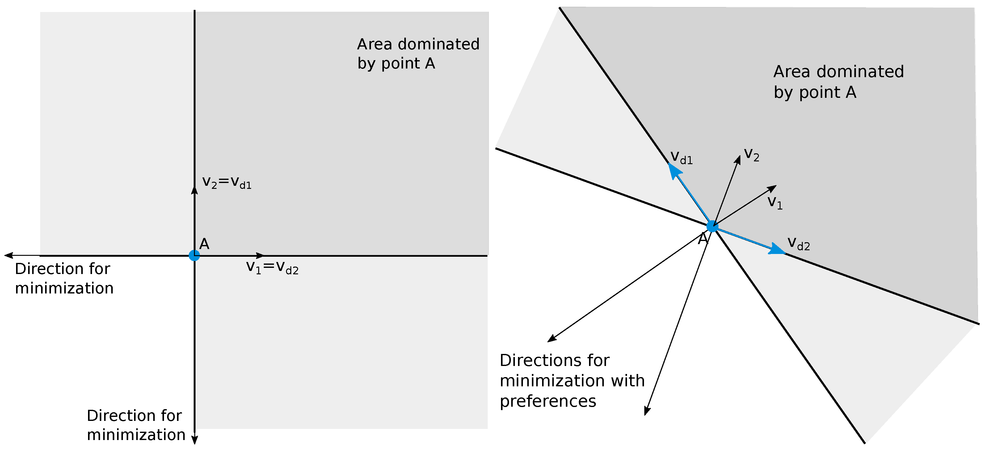
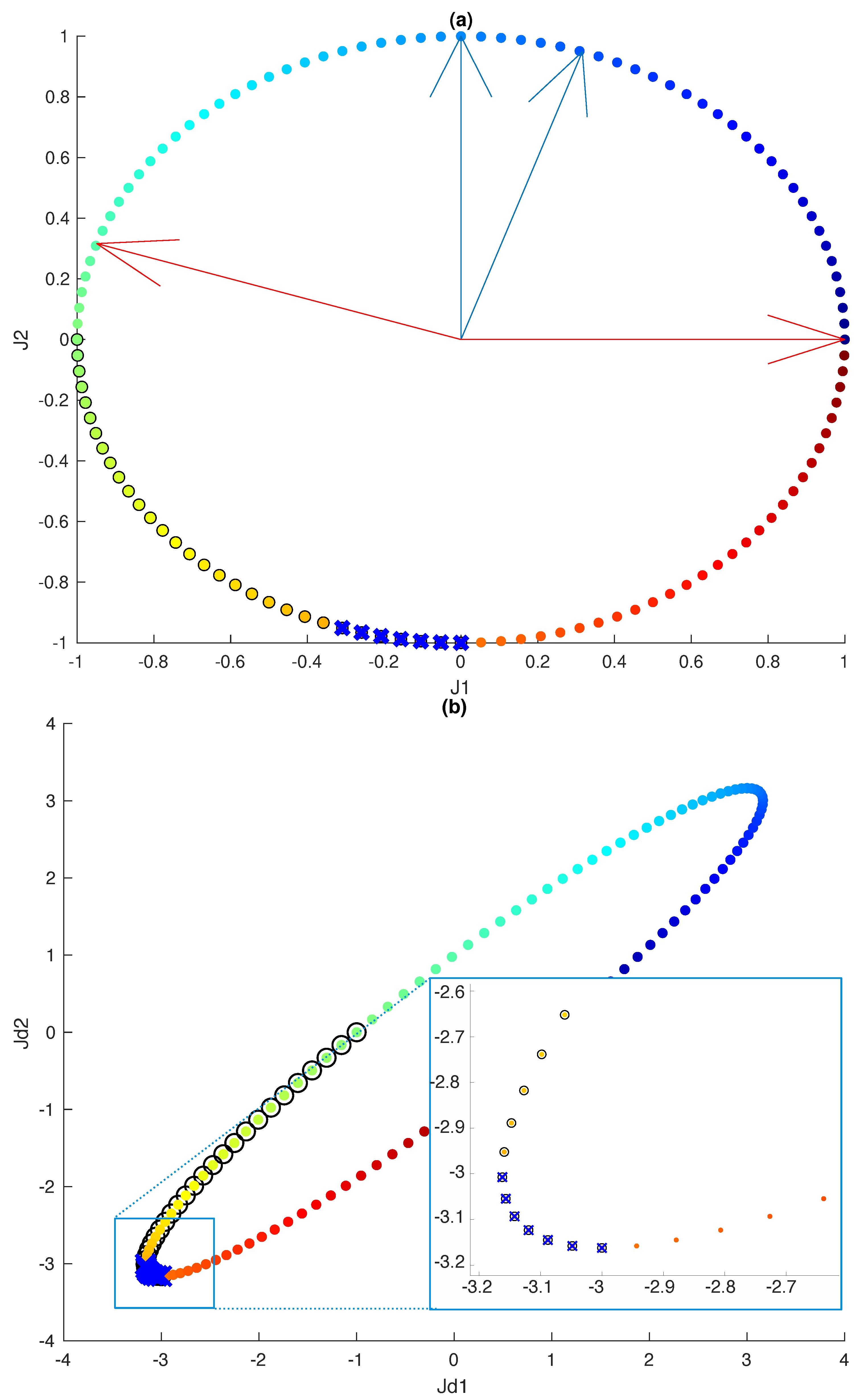
Figure 1 shows an example of the reinterpretation of dominance for a 2-objective space. The figure shows the canonical interpretation of dominance and how the dominance area changes when a different basis of preference directions is considered. Note that the effect of considering the dominance defined by the cone generated by ${\mathcal{B}}_d$ can be understood as a deformation of the area that is dominated by a given point. Remark that, if the canonical base is set as the preference basis, the dominance basis is also the canonical basis (dominance and preference basis are the same). In the next subsection, we will provide the equations to obtain the dominance basis ${\mathcal{B}}_d$ from the preference directions basis.

Computation of Dominance Basis ${\mathcal{B}}_d$

Let $({\mathbb{R}}^n,\parallel ·{\parallel }_2)$ be the n-dimensional Euclidean space. Consider a basis ${\mathcal{B}}_p:=\{v_i:i=1,...,n\}$ norm one elements of ${\mathbb{R}}^n$ included in the positive cone of ${\mathbb{R}}^n$. Each of the elements of the basis defines what we have called a preference direction for the optimization. The optimization procedure that we present here proposes to consider the associated dominance cone as the set of all vectors that are over the hyperplane defined by each vector defining a preference direction (its projection on this vector must be positive). Therefore, we define the positive semispace $S_{v_i}^{+}$ associated with the preference direction $v_i,$ $i=1,...,n,$ as

$$S_{v_i}^{+}:=\{v\in {\mathbb{R}}^n:v·v_i\ge 0\}.$$

Consequently, the dominance cone $C_d^{+}$ can be defined as follows.

Definition 1.

Let ${\mathcal{B}}_p:=\{v_i:i=1,...,n\}$ be a basis of preference directions of ${\mathbb{R}}^n.$ We define the dominance cone as the intersection of all the semispaces $S_{v_i}^{+},$ that is:

$$C_d^{+}:=\bigcap _{i=1}^n{S}_{v_i}^{+}=\left\{v\in {\mathbb{R}}^n:v·v_i\ge 0,i=1,...,n\right\}.$$

The positive cone $C_d^{+}$ generated by ${\mathcal{B}}_p$ allows to reinterpret dominance according to the new preference directions: if A is a point in ${\mathbb{R}}^n,$ $A+C_d^{+}$ gives the set of all the points that are dominated by A. In Figure 1, a 2D example is given, where the dark grey area shows the area dominated by point A, that is, $A+C_d^{+}$.

Definition 2.

Given a set of vectors $Z=\{z_1,...,z_m\}\subset {\mathbb{R}}^n,$ we define its positive linear hull as the set

$$Pos\left(Z\right):=\left\{\sum _{i=1}^m{\lambda }_i{z}_i:{\lambda }_i\ge 0\right\}.$$

For the subsequent proposals described in Section 3.2, it is necessary to obtain the dominance basis ${\mathcal{B}}_d$ corresponding to the preference basis ${\mathcal{B}}_p$ defined by the DM. A way to obtain ${\mathcal{B}}_d$ is based on the equivalence of $C_d^{+}$ and $Pos\left({\mathcal{B}}_d\right)$ (see Proposition 1). As we already mentioned, the dominance basis is defined by vectors that are orthogonal to vectors of the preference basis.

Proposition 1.

The dominance cone associated with a basis of preference directions ${\mathcal{B}}_p=\{v_i:i=1,...,n\}$ coincides with the positive linear hull $Pos\left({\mathcal{B}}_d\right)$ of the set of vectors ${\mathcal{B}}_d:=\{v_{di}:i=1,...,n\}$ defined as follows.

For every $i=1,...,n,$ $v_{di}\in {\mathbb{R}}^n$ is a (norm one) solution of the system

$$\left[\begin{array}{c}{v}_1·v_{di}=0\\ ⋮\\ v_{i-1}·v_{di}=0\\ v_{i+1}·v_{di}=0\\ ⋮\\ v_n·v_{di}=0\end{array}\right]$$

which also satisfies that $v_i·v_{di}>0.$

Proof. 

First, note that for each $i=1,...,n,$ the linear system defined above always has a subspace of solutions of dimension 1, because it is made of $n-1$ linear equations. So, we can choose a solution with norm equal to one, and also $v_i·v_{di}>0$ (if $v_i·v_{di}=0$ for all i, then $v_{di}=0$, since ${\mathcal{B}}_p$ is a basis).

Let us prove first that $C_d^{+}\subseteq Pos\left({\mathcal{B}}_d\right).$ Take an element $v\in C_d^{+}.$ By the definition of the set of preference directions—they are linearly independent—, we have that the set $\{v_{d1},...,v_{dn}\}$ defined as in the statement of the result, is a basis for ${\mathbb{R}}^n.$ Then, v can be written as $v={\sum }_{i=1}^n{x}_i{v}_{di}$, for real numbers $x_1,...,x_n.$ We have that

$$0\le v·v_k=\sum _{i=1}^n{x}_i{v}_{di}·v_k=x_k{v}_{dk}·v_k$$

for all $k=1,...,n.$ Since $v_{dk}·v_k>0$, we get that $x_k\ge 0.$ This can be done for all $k=1,...,n$, and so we get that $C_d^{+}\subseteq Pos\left({\mathcal{B}}_d\right).$

Conversely, take an element $v\in Pos\left({\mathcal{B}}_d\right).$ Then, it can be written as $v={\sum }_{i=1}^n{x}_i{v}_{di},$ where all the coordinates $x_i$ are non-negative. Then,

$$v·v_k=\sum _{i=1}^n{x}_i{v}_{di}·v_k=x_k{v}_{dk}·v_k.$$

But $x_k\ge 0$ and $v_{dk}·v_k\ge 0,$ and so $v·v_k\ge 0$ for all k. Consequently, $v\in C_d^{+}$, and so $Pos\left({\mathcal{B}}_d\right)\subseteq C_d^{+}.$

Therefore, $Pos\left({\mathcal{B}}_d\right)=C_d^{+},$ and the result is proved. □

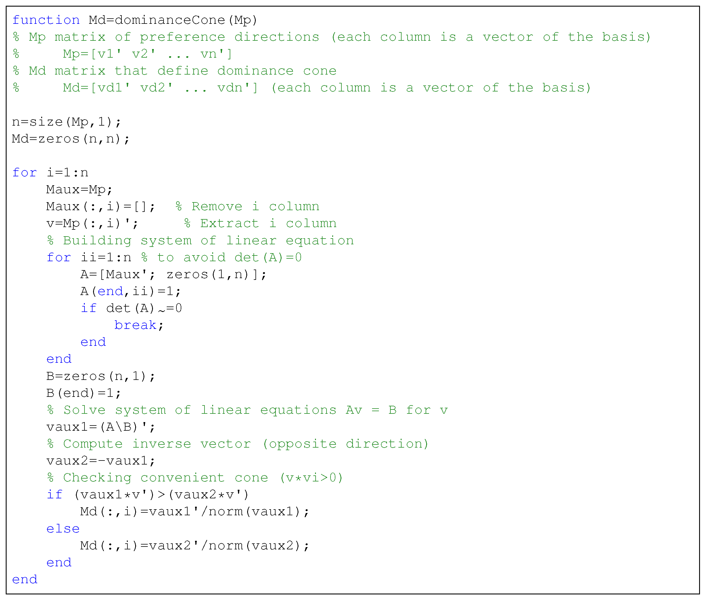
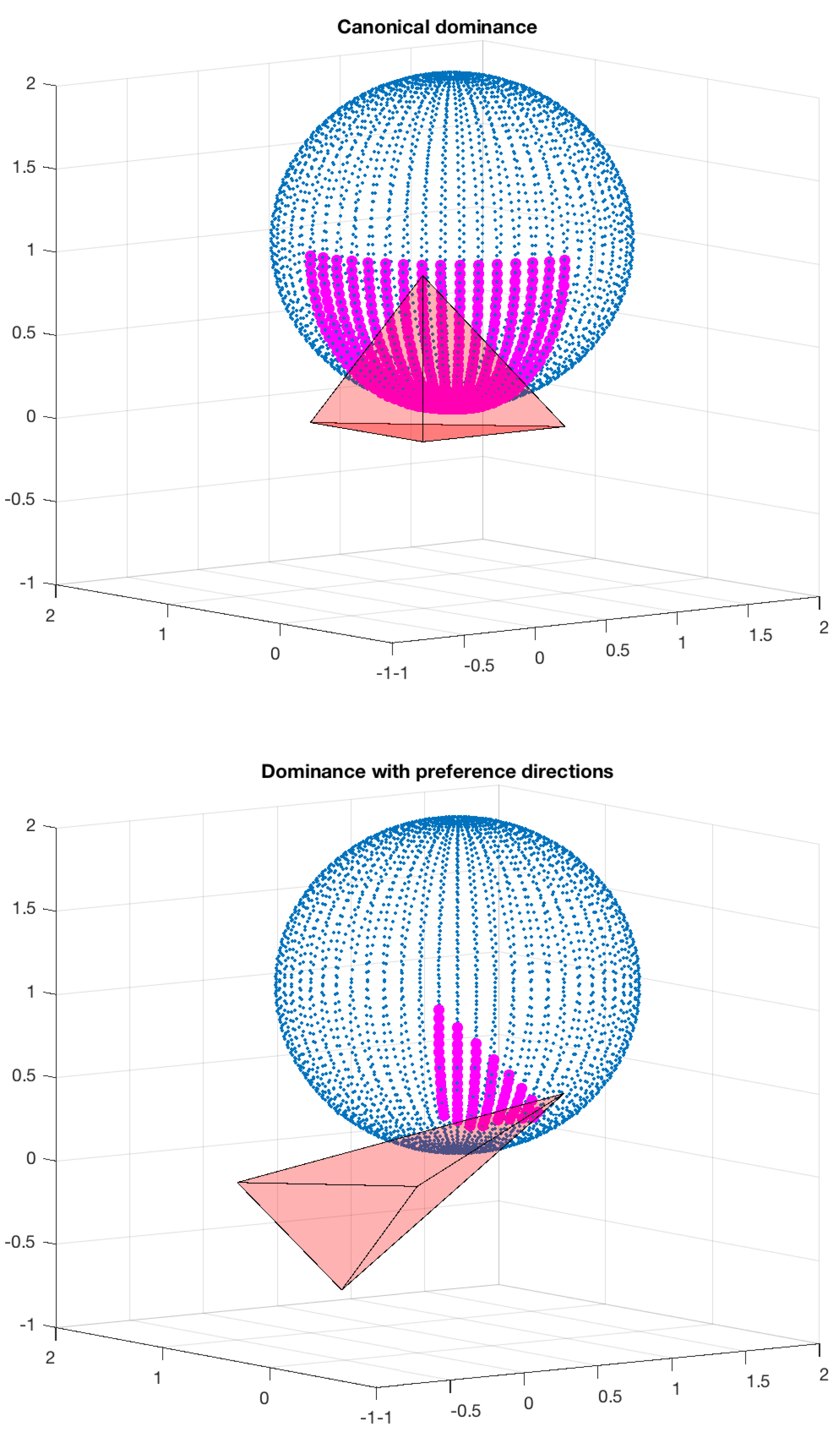
Based on Proposition 1, it is possible to give an algorithm that computes the vectors of the corresponding dominance basis ${\mathcal{B}}_d$. An example with MATLAB is shown in Figure 2.

3. Using Preference Directions in Multi-Objective Optimization Problems

There are two direct uses of the dominance bases:

• Including preferences in the decision-making step.
• Including preferences by reformulating the optimization problem.

In both cases, the mathematical meaning underlying the concept of “optimization direction" refers to the definition of preference basis. From this basis, it is possible to obtain the dominance basis—as described in the previous section—which is the one that redefines the space of objectives, thus incorporating the preferences.

3.1. Including Preferences in the Decision Making Step

As a first application, we consider the case of a DM who is provided with a Pareto front and tries to select a solution based on his preferences. In this selection process, graphical tools are important to visually analyze the Pareto front. A standard way used is to color the different points of the Pareto front according to the designer’s preferences [17].

To illustrate this use, a 2D example is shown below. Let us suppose that all possible solutions of a 2D multi-objective problem are placed on a disc of radius r = 1, and centered on the origin. Obviously, the perimeter of this set of solutions is formed by the circle of radius unit centered on the origin (see Figure 3a). If the optimization problem consists on minimizing both objectives, it is easy to locate the Pareto front, represented as a discrete approach formed by the points highlighted in black in Figure 3a. Once the Pareto front is obtained, the DM usually has to choose one of the solutions included in the front. Assuming that both objectives are equally relevant, it seems reasonable to select a solution close to the ideal point. The ideal point has the minimum possible value for each objective, which is highlighted with a diamond in Figure 3b. A commonly used tool in the decision phase is to color the points of the Pareto front according to their proximity to the designer’s preferred area. In the case of Figure 3b, the points closest to the ideal point are colored dark blue, and the furthest points are colored red.

However, if the DM defines some preference directions, the analysis of the solutions of the Pareto front changes. If we suppose that ${\mathcal{B}}_p$ is defined by the DM, ${\mathcal{B}}_d$ can be easily obtained applying the algorithm provided by Proposition 1:

$${\mathcal{B}}_p=\left\{\begin{array}{cc}{v}_1=& (0.3162,0.9487)\hfill \\ v_2=& (0,1)\hfill \end{array}\right\}\to {\mathcal{B}}_d=\left\{\begin{array}{cc}{v}_{d1}=& (1,0)\hfill \\ v_{d2}=& (-0.9487,0.3162)\hfill \end{array}\right\}.$$

(1)

With this new base, which incorporates the DM’s preferences, the objective space is deformed by affecting the distances between points. With the associated dominance basis ${\mathcal{B}}_d$ and the matrix $M_d$, the new distances are easily calculated (see Appendix A). Figure 4a shows, in the canonical space, the Pareto front colored according to the proximity to the ideal point with the new ${\mathcal{B}}_d$ base. In the same figure, the vectors of the ${\mathcal{B}}_p$ preference base (in blue color) are shown, as well as the vectors corresponding to the ${\mathcal{B}}_d$ dominance base (in red color). In addition, to better understand how the relationship of distances to the ideal point has been changed, Figure 4b is shown. In this figure, the Pareto front and the ideal point in the space defined by ${\mathcal{B}}_d$ are represented.

As seen in the figure, this simple preference-based coloring allows the DM to select a subset of relevant solutions according to his preferences.

3.2. Including Preferences by Reformulating the Optimization Problem

This way of considering preferences—by selecting a new basis—is easy to apply with all the available optimization tools because it is just a change of coordinates. Defining a multi-objective problem as:

$$\begin{array}{ccc}\hfill & & \underset{\theta }{min}J\left(\theta \right)\hfill \\ \hfill \mathrm{subject}\mathrm{to}:& & \theta \in S\subset {\mathbb{R}}^m,\hfill \end{array}$$

(2)

where $\theta =({\theta }_1,\cdots ,{\theta }_m)\in {\mathbb{R}}^m$ is the decision vector, $J\left(\theta \right)=(J_1\left(\theta \right),\cdots ,J_n\left(\theta \right))\in {\mathbb{R}}^n$ is objective vector, and S is the subspace that satisfies all the additional constraints of the problem.

We must define a new basis that collects the preference directions:

$${\mathcal{B}}_p:=\{v_i:i=1,...,n\}.$$

(3)

The redefinition of the multi-objective optimization problem that include preferences is done using the associated dominance basis ${\mathcal{B}}_d:=\{v_{di}:i=1,...,n\}$ and the matrix $M_d$ (see Equation (A1), Appendix A):

$$\begin{array}{ccc}\hfill & & \underset{\theta }{min}{J}_d\left(\theta \right)\hfill \\ & & J_d\left(\theta \right)={\left(M_d^{-1}J{\left(\theta \right)}^T\right)}^T\hfill \\ \hfill \mathrm{subject}\mathrm{to}:& & \theta \in S\subset {\mathbb{R}}^m.\hfill \end{array}$$

(4)

To see the effect of the preference directions in the optimization problem, an example of a 2D problem (in the objective space) is shown. It is assumed that the space of possible objectives is on a disk of unit radius. Figure 5a shows the periphery of this set on a canonical basis, while Figure 5b shows the same circle but at the base ${\mathcal{B}}_d$. It is clearly shown how the circle is deformed and becomes an ellipse. The equivalent points have been colored identically in both figures to make them easier to locate.

Figure 5a also shows the vectors that correspond to the preferences base (in blue) and to the dominance base (in red). Note that Pareto front changes according to the base on which the points are represented. The points that correspond to an approximation of the front that would be obtained using the canonical base are highlighted with circles, and the points of the front that would be obtained using the dominance base ${\mathcal{B}}_d$ are marked with “x”. It can be seen that the use of this basis allows the front to be focused on the area preferred by the DM, which has been previously defined by ${\mathcal{B}}_p$. As a additional comment, it can be observed that by focusing on the region of interest, in general fewer solutions are obtained. This facilitates the final decision stage, since the DM has to choose between fewer options but all oriented according to his preferences.

Therefore, the use of ${\mathcal{B}}_d$ directly in the formulation of the optimization problem provides the pertinency property without having to modify the optimization algorithm. This methodology can be used with any optimizer since it only involves a reformulation of the optimization problem.

A 3D example comparing canonical dominance and dominance with preferences is shown in Figure 6. For demonstration purposes, the set of possible objective values is a sphere, and the boundary of the sphere is represented in blue. The basis ${\mathcal{B}}_p$ defines the dominance cone ${\mathcal{B}}_d$. Remark that, if ${\mathcal{B}}_p$ is the canonical base, ${\mathcal{B}}_p={\mathcal{B}}_d$.

$${\mathcal{B}}_p=\left\{\begin{array}{cc}{v}_1=& (1,0,0)\hfill \\ v_2=& (0,1,0)\hfill \\ v_3=& (0,0,1)\hfill \end{array}\right\}\to {\mathcal{B}}_d=\left\{\begin{array}{cc}{v}_{d1}=& (1,0,0)\hfill \\ v_{d2}=& (0,1,0)\hfill \\ v_{d3}=& (0,0,1)\hfill \end{array}\right\}.$$

(5)

The dominance cone defined by ${\mathcal{B}}_d$ is represented with a polyhedron with one of its vertex at the origin. Each of the edges starting at the origin represents a vector of ${\mathcal{B}}_d.$ The polyhedron is colored in red. The resulting Pareto front has been highlighted in magenta.

Figure 6 shows the resulting Pareto front for canonical dominance (upper figure) and Pareto front obtained with a base of preferences defined by ${\mathcal{B}}_p$ (bottom figure):

$$\begin{array}{c}\hfill {\mathcal{B}}_p=\left\{\begin{array}{cc}{v}_1=& (0,0.7071,0.7071)\hfill \\ v_2=& (0.5774,0.5774,0.5774)\hfill \\ v_3=& (0.7071,0.7071,0)\hfill \end{array}\right\}\to \\ \hfill {\mathcal{B}}_d=\left\{\begin{array}{cc}{v}_{d1}=& (-0.7071,0.7071,0)\hfill \\ v_{d2}=& (0.5774,-0.5774,0.5774)\hfill \\ v_{d3}=& (0,0.7071,-0.7071)\hfill \end{array}\right\}.\end{array}$$

(6)

The reader can notice how the selection of preference directions provides a narrower Pareto set when comparing with the canonical situation. Indeed, the preference direction basis ${\mathcal{B}}_p$ is strictly included in the canonical positive cone, what provides a wider dominance cone (see the picture on the bottom of Figure 6). This means that, in the new situation, each point in the Pareto front dominates more points of the original sphere of objective values, what gives a smaller set of dominating relevant points. To understand the deformation produced by the preferences, Figure 7 shows the same that Figure 6 (bottom) but drawn in ${\mathcal{B}}_p$ basis. The DM has to consider a smaller set of optimal points for his final election, all of them fitting with his original preference requirements.

4. Application Example: The Daily Diet Design Problem

In this section, we will develop a complete example regarding the design of a healthy diet. The original problem can be found in Reference [18], where an alternative form of decision-making called TOPSIS is presented. The methodology tries to reach the compromise that the chosen alternative should have the smallest distance from the positive ideal solution and the largest distance from the negative ideal solution. Therefore, no preferences are proposed by the DM and cannot be compared with the proposal of the present work. In order to illustrate the methodology, we will propose some DM preferences.

The problem concerns the prescription of a diet for a patient who has some particular health characteristics. Suppose that the decision variables with their bound constraints are the following.

• Milk pints: $0.0\le x1\le 6.00.$
• Beef pounds: $0.0\le x2\le 1.00.$
• Eggs dozen: $0.0\le x3\le 0.25.$
• Bread ounces: $0.0\le x4\le 10.00.$
• Lettuce and salad ounces: $0.0\le x5\le 10.00.$
• Orange juice pints: $0.0\le x6\le 4.00.$

The problem has three design objectives, $J1,J2$ and $J3$:

$$\begin{array}{c}{J}_1\left(x\right)=24x_1+27x_2+15x_4+1.1x_5+52x_6\hfill \\ J_2\left(x\right)=10x_1+20x_2+120x_3\hfill \\ J_3\left(x\right)=0.22x_1+2.2x_2+0.8x_3+0.1x_4+0.05x_5+0.26x_6\hfill \end{array},$$

(7)

where $J_1\left(x\right)$ is the Carbohydrate intake [g], $J_2\left(x\right)$ is the Cholesterol intake [unit], and $J_3\left(x\right)$ is the Cost [$].

There are also some constraints that affects the optimization calculations, regarding the amount of vitamin A [i.u] ($g_1\left(x\right)$), iron [mg] ($g_2\left(x\right)$), food energy [calories] ($g_3\left(x\right)$), and proteins [g] ($g_4\left(x\right)$).

$$\begin{array}{c}{g}_1\left(x\right)=720x_1+107x_2+7080x_3+134x_5+1000x_6\ge 5000\hfill \\ g_2\left(x\right)=0.2x_1+10.1x_2+13.2x_3+0.75x_4+0.15x_5+1.2x_6\ge 12.5\hfill \\ g_3\left(x\right)=344x_1+1460x_2+1040x_3+75x_4+17.4x_5+240x_6\ge 2500\hfill \\ g_4\left(x\right)=18x_1+151x_2+78x_3+2.5x_4+0.2x_5+4.0x_6\ge 63\hfill \end{array}$$

(8)

The multi-objective problem to be solved can be written as follows:

$$\begin{array}{ccc}\hfill \underset{x}{min}J\left(x\right)& & \\ & & J\left(x\right)=(J_1\left(x\right),J_2\left(x\right),J_3\left(x\right))\in {\mathbb{R}}^3\hfill \\ \hfill \mathrm{subject}\mathrm{to}:& & \underline{x}\le x\le \overline{x},x\in {\mathbb{R}}^6\hfill \\ & & g_i\left(x\right)\ge b_i,i=1\cdots 4,g_i\left(x\right)\in \mathbb{R},b_i\in \mathbb{R}.\hfill \end{array}$$

(9)

Since it is a linear problem in both objectives and constraints, a classic optimization method obtains good results with a reasonable computational cost. Pareto front is obtained using a classic method, $ϵ$-constraint method, described in Reference [16]. Pareto front values are achieved by solving multiple mono-objective problems in which only one of the objectives is minimized, and the rest are considered as constraints. In order to obtain a suitable discretization of the front, it is necessary to vary the value of these constraints on the objectives in an adequate way. The steps are the following: first, the minimums of each independent objective are obtained. With these values we have the range of values where approximately the Pareto front is located. Subsequently, the increase to be applied to the restriction in each mono-objective problem is defined. In this particular case, the range of variation of two of the objectives ($J_1$ y $J_3$) has been divided into 50 parts, obtaining $ϵJ1$ y $ϵJ3$. Subsequently, multiple problems of a single objective are solved by adding constraints on the other objectives. Then, multiple problems ($50\times 50=$ 2500) of a single objective are solved by adding constraints on the other objectives, that is, varying n from 1 to 50 and m from 1 to 50, and solving the following mono-objective problems:

$$\begin{array}{ccc}\hfill \underset{x}{min}{J}_2\left(x\right)& & \\ \hfill \mathrm{subject}\mathrm{to}:& & \underline{x}\le x\le \overline{x},x\in {\mathbb{R}}^6\hfill \\ & & g_i\left(x\right)\ge b_i,i=1\cdots 4,g_i\left(x\right)\in \mathbb{R},b_i\in \mathbb{R}\hfill \\ & & J_1\left(x\right)\le J{1}_{min}+ϵJ1·n\hfill \\ & & J_1\left(x\right)\le J{3}_{min}+ϵJ3·m.\hfill \end{array}$$

(10)

If a better approach to the front is required, the process can be repeated minimizing $J_1\left(x\right)$ or $J_3\left(x\right)$.

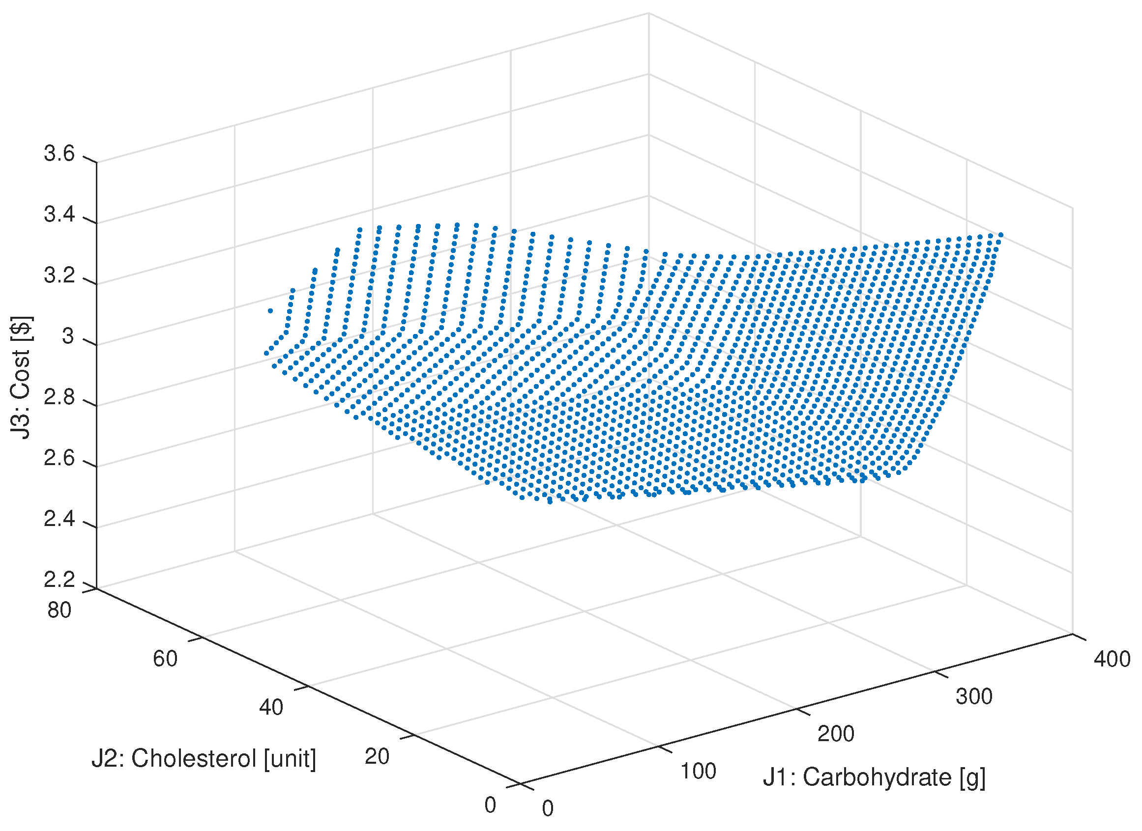
Since the problem is linear in both the target and the constraints, linear programming has been used. The approximation to the front obtained consists of 2049 points. Twenty-five hundred mono-objective problems have been executed, but some of them were not feasible; therefore, they did not provide a solution. Figure 8 shows a 3D representation of the Pareto front approximation obtained.

The DM must analyze this front and select a solution that fits his preferences. The first step, to have fewer points to choose from, is to reduce the number of points to 342 while maintaining a good representation of the front. This can be done reducing the discretization step.

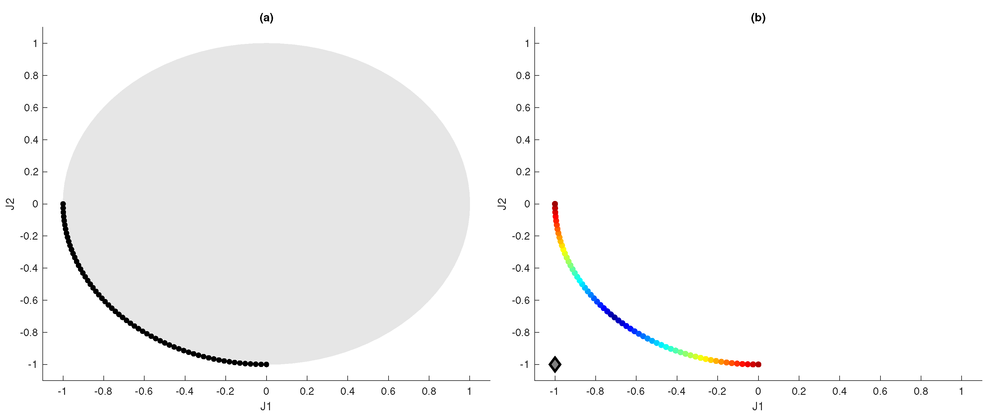
Then, to help in the decision-making, the Pareto front is colored according to distance to the ideal point; see Figure 9 (upper). The ideal point corresponds to a possible solution obtained with the minimum values of each of the objectives.

This representation shows to the DM which are the points that present a more ’balanced’ compromise between objectives. It should be noted that, in order to calculate the distance to the ideal point, the front has been scaled trying to avoid the distortions that can be caused by the different units and orders of magnitude of each of the objectives. Each objective is rescaled between 0 and 1. With these new values, the distances to the ideal point are calculated (that corresponds to the point $(0,0,0)$ when applying the scaling).

This ’balanced’ solution is not always the preferred one, and the DM can decide on another order of preferences. It is very useful that these preferences will be incorporated in all phases of the MO problem resolution. In this case, a set of preferences defined by a vector base will be established.

Let us show now how to implement the preference directions by the DM, in this case, the doctor who treats the patient with special needs. Concretely, the doctor knows that the diet for the patient must satisfy preferably the following relations:

• The ratio among the Carbohydrate intake and the Cholesterol intake must be as near as possible to 2. This means that the preference equation $J1=2·J2$ must be taken into account. This condition supplies one of the preference directions: $v_1=(2,1,0)$.
• Since there are a lot of bad quality Carbohydrates in the market, the doctor wants to promote the use of the correct ones.
  An indirect way to increase the use of good quality carbohydrates is through cost. It is estimated that the impact on the price of the diet of such carbohydrates is around 1$ per 100 g of carbohydrates. Poor quality carbohydrates are significantly cheaper on the market. This allows to set a new direction of preference that is $J1/100=J3$. This second conditions supplies another preference direction: $v_2=(1/100,0,1)$.
• The third preference direction maintains the original objective of minimizing cost: $v_3=(0,0,1)$.

Summing up all these assumptions and converting these vectors into unit vectors the preference basis ${\mathcal{B}}_p$ and its corresponding dominance basis are:

$$\begin{array}{c}\hfill {\mathcal{B}}_p=\left\{\begin{array}{cc}{v}_1=& (0.8944,0.4472,0)\hfill \\ v_2=& (0.01,0,1)\hfill \\ v_3=& (0,0,1)\hfill \end{array}\right\}\to \\ \hfill {\mathcal{B}}_d=\left\{\begin{array}{cc}{v}_{d1}=& (0,1,0)\hfill \\ v_{d2}=& (0.4472,-0.8944,0)\hfill \\ v_{d3}=& (-0.4472,0.8944,0.0045)\hfill \end{array}\right\}\end{array}.$$

(11)

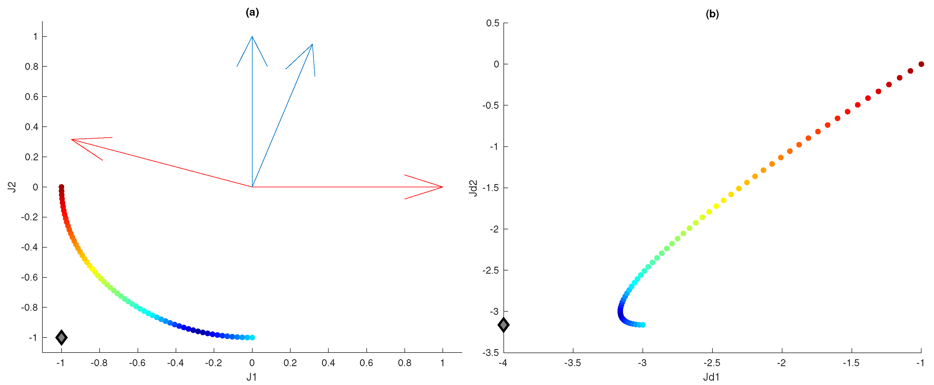
By changing the base, the calculation of the distances is modified. The example shows how the ’color’ of the solutions closest to the ideal changes when these preferences are incorporated; see Figure 9 (bottom).

It can be seen that coloring, considering these new preferences (see Figure 9 (bottom)), orients the DM towards a different area of the front. Usually, these points would be more interesting for DM, and, consequently, he could choose more suitable solutions.

Table 1. alt1: The five nearest points to ideal point without considering preferences. alt2: The five nearest points to ideal point considering preferences.

Sol	${\mathit{J}}_1$	${\mathit{J}}_2$	${\mathit{J}}_3$	${\mathit{x}}_1$	${\mathit{x}}_2$	${\mathit{x}}_3$	${\mathit{x}}_4$	${\mathit{x}}_5$	${\mathit{x}}_6$
alt1	236.87	39.51	2.85	1.78	0.69	0.07	0.69	0	3.17
	222.52	42.66	2.85	1.81	0.72	0.08	0.17	0	3.02
	236.87	35.97	2.91	1.60	0.74	0.04	0	0.24	3.43
	251.22	36.36	2.85	1.76	0.65	0.05	1.22	0	3.33
	222.52	39.79	2.91	1.74	0.74	0.06	0	1.13	3.07
alt2	236.87	69.26	2.36	3.52	0.21	0.25	7.40	0	0.68
	222.52	68.69	2.42	3.33	0.30	0.24	6.04	0	0.84
	281.67	67.83	2.24	3.78	0	0.25	10.00	0	0.79
	265.57	66.68	2.30	3.68	0.09	0.23	9.29	0	0.68
	251.22	66.11	2.36	3.50	0.18	0.23	7.92	0	0.84

shows the five best solutions extracted from each of the colored fronts. In particular, the points closest to the ideal point are shown. As you can see, the solutions obtained from coloring with preferences are closer to the preferences of the DM. The cost is lower, ratios among the Carbohydrate intake and the Cholesterol intake are nearest to two and ratios among Carbohydrate intake and Cost are nearest to 100. In this first case, the preference directions are used in the decision phase to assist the DM in making the final decision. This procedure does not reduce the number of solutions to be evaluated but enables a very simple way to visualize the results and select a subset of solutions of interest.

Another alternative is to use the preference directions in the optimization process itself as proposed in Equation (4). The same multi-objective optimization method has been used to obtain the new front (constraint method). In this case, the range of variation of two of the objectives ($J_{d1}$ and $J_{d3}$) has been divided into 10 parts and $10\times 10=100$ mono-objective problems have been solved. The Pareto front achieved has 10 points (many of the mono-objective problems raised were not feasible and, therefore, did not provide a solution). Applying the preferences to modify the optimization problem has significantly reduced the computational cost and has focused the solution to the area of interest.

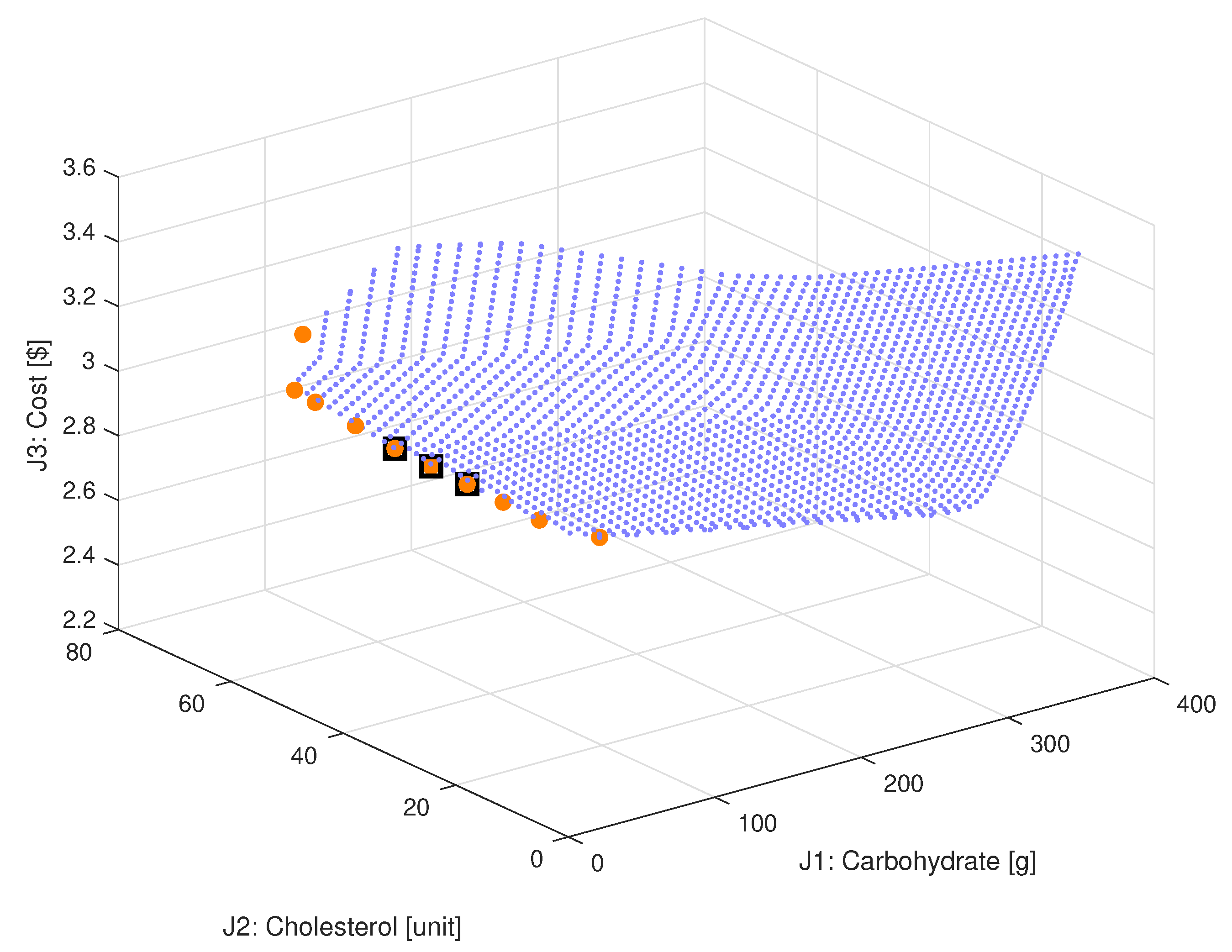
Figure 10 shows the new front obtained compared to the previous one (Figure 8), the new front is colored in orange. There is a noticeable difference, since now the preferences have deformed the target space and have oriented the search towards a different zone adjusted to the DM’s preferences. It should be noted that the number of points of the front obtained is 10, which is significantly lower than the number of points obtained in the original front without considering preferences (2049 points). Among these new values, the DM can select, for example, a more balanced solution. The points highlighted with black square in the figure show 3 examples of balanced solutions. The particular values of this 3 solutions are shown in

Table 2. Balanced solutions obtained from the Pareto front with preferences.

${\mathit{J}}_1$	${\mathit{J}}_2$	${\mathit{J}}_3$	${\mathit{x}}_1$	${\mathit{x}}_2$	${\mathit{x}}_3$	${\mathit{x}}_4$	${\mathit{x}}_5$	${\mathit{x}}_6$
151.65	70.34	2.65	2.66	0.69	0.25	0.31	0	1.24
175.46	70.13	2.57	2.91	0.55	0.25	2.31	0	1.08
199.27	69.91	2.49	3.15	0.42	0.25	4.31	0	0.92

.

5. Conclusions

This work shows a very easy alternative to introduce preferences both in the optimization problem formulation and/or in the final decision phases. The methodology is based on defining vectors that mark the directions of optimization and constitute what is called the preference base. It is shown and formally demonstrated how to obtain the dominance base from the preference one. In addition, the MATLAB code is provided for its calculation. This base is the one used to redefine the dominance relations, and it is the one in charge of ’deforming’ the space to include the defined preferences. In Section 3, it is shown that the deformation of the space resulting from applying the dominance basis reconfigures the problem so that the points in the directions of preference dominate the rest of the solutions. This deformation is usable both to redefine the concept of dominance (this feature is usable by optimization algorithms) and to recalculate the distances that reorder the points in the space according to the preferences (this feature can be used in the decision phase to order solutions).

An important advantage of this methodology, when applied in the problem reformulation, is it can be used with any multi-objective optimization algorithm. In order to prove the use and usefulness of this methodology, a problem with three objectives has been raised. The results obtained show the simplicity of the use of this methodology and opens up a new range of possibilities for the inclusion of preferences. It has not been the objective of this work to show a general methodology for defining the directions of preferences; this aspect is particular to each problem and opens a very interesting research line that would allow to popularize the use of the methodology proposed in this article.

References

1. Wang, H.; Olhofer, M.; Jin, Y. A mini-review on preference modeling and articulation in multi-objective optimization: Current status and challenges. Complex Intell. Syst. 2017, 3, 233–245. [Google Scholar] [CrossRef]
2. López-Jaimes, A.; Coello, C.A.C. Including preferences into a multiobjective evolutionary algorithm to deal with many-objective engineering optimization problems. Inf. Sci. 2014, 277, 1–20. [Google Scholar] [CrossRef]
3. Coello, C.A.C. Handling preferences in evolutionary multiobjective optimization: A survey. In Proceedings of the 2000 Congress on Evolutionary Computation, CEC00 (Cat. No.00TH8512), La Jolla, CA, USA, 16–19 July 2000; Volume 1, pp. 30–37. [Google Scholar] [CrossRef]
4. Bechikh, S.; Kessentini, M.; Said, L.B.; Ghédira, K. Preference Incorporation in Evolutionary Multiobjective Optimization. In Advances in Computers; Elsevier: Amsterdam, The Netherlands, 2015; Chapter 4; pp. 141–207. [Google Scholar] [CrossRef]
5. Deb, K.; Sundar, J. Reference point based multi-objective optimization using evolutionary algorithms. In Proceedings of the 8th Annual Conference on Genetic and Evolutionary Computation—GECCO’06, Seattle, DC, USA, 8–12 July 2006; ACM Press: New York, NY, USA, 2006. [Google Scholar] [CrossRef] [Green Version]
6. Reynoso-Meza, G.; Sanchis, J.; Blasco, X.; García-Nieto, S. Physical programming for preference driven evolutionary multi-objective optimization. Appl. Soft Comput. 2014, 24, 341–362. [Google Scholar] [CrossRef] [Green Version]
7. Messac, A. Physical programming—Effective optimization for computational design. AIAA J. 1996, 34, 149–158. [Google Scholar] [CrossRef]
8. Reynoso-Meza, G. Controller Tuning by Means of Evolutionary Multiobjective Optimization: A Holistic Multiobjective Optimization Design Procedure. Ph.D. Thesis, Universitat Politècnica de València, Camino de Vera s/n, Valencia, Spain, 2014. [Google Scholar] [CrossRef]
9. Sanchis, J.; Martínez, M.A.; Blasco, X. Integrated multiobjective optimization and a priori preferences using genetic algorithms. Inf. Sci. 2008, 178, 931–951. [Google Scholar] [CrossRef]
10. Cruz-Reyes, L.; Fernandez, E.; Sanchez, P.; Coello Coello, C.A.; Gomez, C. Incorporation of implicit decision-maker preferences in multi-objective evolutionary optimization using a multi-criteria classification method. Appl. Soft Comput. 2017, 50, 48–57. [Google Scholar] [CrossRef]
11. Liu, R.; Li, J.; Feng, W.; Yu, X.; Jiao, L. A new angle-based preference selection mechanism for solving many-objective optimization problems. Soft Comput. 2018, 22, 6311–6327. [Google Scholar] [CrossRef]
12. Sagawa, M.; Kusuno, N.; Aguirre, H.; Tanaka, K.; Koishi, M. Evolutionary Multiobjective Optimization including Practically Desirable Solutions. Adv. Oper. Res. 2017, 2017, 1–16. [Google Scholar] [CrossRef] [Green Version]
13. Thiele, L.; Miettinen, K.; Korhonen, P.J.; Molina, J. A Preference-Based Evolutionary Algorithm for Multi-Objective Optimization. Evol. Comput. 2009, 17, 411–436. [Google Scholar] [CrossRef] [PubMed]
14. Li, K.; Chen, R.; Min, G.; Yao, X. Integration of Preferences in Decomposition Multiobjective Optimization. IEEE Trans. Cybern. 2018, 48, 3359–3370. [Google Scholar] [CrossRef] [PubMed] [Green Version]
15. Zou, J.; He, Y.; Zheng, J.; Gong, D.; Yang, Q.; Fu, L.; Pei, T. Hierarchical preference algorithm based on decomposition multiobjective optimization. Swarm Evol. Comput. 2021, 60, 100771. [Google Scholar] [CrossRef]
16. Miettinen, K.M. Nonlinear Multiobjective Optimization; Kluwer Academic Publishers: New York, NY, USA, 1998. [Google Scholar] [CrossRef]
17. Blasco, X.; Herrero, J.M.; Sanchis, J.; Martínez, M. A new graphical visualization of n-dimensional Pareto front for decision-making in multiobjective optimization. Inf. Sci. 2008, 178, 3908–3924. [Google Scholar] [CrossRef]
18. Hwang, C.L.; Lai, Y.J.; Liu, T.Y. A new approach for multiple objective decision making. Comput. Oper. Res. 1993, 20, 889–899. [Google Scholar] [CrossRef]
Figure 1. Graphical interpretation of canonical dominance and dominance with preferences. Dominated area by point A for different dominance basis ( v d 1 , v d 2 ). Dominance with the canonical basis (figure on the left) and dominance when preferences are included with a basis change (figure on the right).
Mathematics 09 00991 g001
Figure 2. MATLAB function based on proposition 1 that computes dominance basis from preference basis.
Mathematics 09 00991 g002
Figure 3. (a) Possible values of the objectives (grey disc) and approximation to Pareto front (black points). (b) Coloring Pareto front according to proximity to ideal point (diamond).
Mathematics 09 00991 g003
Figure 4. (a) Pareto front colored according to proximity to ideal point computed in the basis B d and plotted in canonical basis. Vectors of preference directions in blue and vectors of dominance directions in red. (b) Same points but plotted in the basis B d .
Mathematics 09 00991 g004
Figure 5. (a) Representation of the unit circle in the canonical basis, and the preference (red) and dominance (blue) vectors of the corresponding basis. Lines with ’o’ and ’x’ show Pareto front in canonical and B d basis, respectively. (b) Same circle and Pareto fronts drawn in B d basis.
Mathematics 09 00991 g005
Figure 6. 3D Pareto front approximation (in magenta) with canonical dominance (upper figure) and dominance with preferences (bottom figure).
Mathematics 09 00991 g006
Figure 7. 3D deformed sphere (blue points) resulting from preferences and Pareto front approximation (in magenta) drawn in B d .
Mathematics 09 00991 g007
Figure 8. Pareto front approximation obtained for daily diet problem.
Mathematics 09 00991 g008
Figure 9. Pareto front obtained for daily diet problem. Upper figure shows the Pareto front colored according to the proximity to ideal point. Figure on the bottom shows the Pareto front colored according to the proximity to ideal point computed in basis B d . In both cases, dark blue color highlights the best solutions (dark red the worst).
Mathematics 09 00991 g009
Figure 10. Pareto front obtained for daily diet problem. In orange, the Pareto front obtained including preferences into the optimization problem resolution. In blue, the original Pareto front obtained without preferences. Black square shows 3 balanced solutions.
Mathematics 09 00991 g010