Abstract
In this paper, we deal with the resolution of a fuzzy multiobjective programming problem using the level sets optimization. We compare it to other optimization strategies studied until now and we propose an algorithm to identify possible Pareto efficient optimal solutions.
1. Introduction
The construction of scientific models to describe real situations represents a significant advance in the aid for decision-making, especially in complex problems. These models allow us to select the essential, discard the accessory, apply scientific knowledge, and, based on them, predict and compare the results of different strategies or decisions. They have proven especially useful when faced with the needs of optimal allocation of resources, evaluation of a system’s performance, obtaining quantitative information for the improvement of processes or their limitations. The study of models where it is necessary to find and identify the best alternative among a collection of possibilities, without having to list and evaluate each explicitly and every one of them constitutes the Optimization Theory’s objective. The situations that allow modeling, where the possible alternatives and the objectives can be expressed and quantified using mathematical functions, constitute a widely studied and applied line of knowledge, known as Mathematical Programming. In particular, Multiobjective Mathematical Programming is really useful in order to model real situations where more than one objective exists.
The growing use of optimization models to help decision-making, in fields as diverse and complex as Economics, Engineering, Social or Life Sciences, has created a demand for new tools that allow considering and solving more real situations, which, in general, do not verify the properties and hypotheses that for classical optimization are essential to ensure an effective search for solutions.
It is quite common to find a certain degree of incomplete, subjective, vague or inaccurate information in the situations to be modeled. The classic mathematical programming tools do not adequately reflect this lack of precision in the data that define both the objective functions and the constraints of the problem. When any of these types of inaccuracies appear in an optimization problem, it cannot be addressed with the classic mathematical optimization tools. Thus, the Fuzzy Set Theory was introduced to manage the imprecision or lack of accurate information that appears in many mathematical models or computations of some real-world phenomena. A significant and growing field is the Fuzzy Optimization that deals with the resolution of optimization problems with imprecise or vague data.
Combining fuzzy and multiobjective optimization tools will help model real problems that cannot be modeled with classic optimization techniques. In the literature, since the first contribution in that sense (Zimmerman [1]), many works can be found where multiobjective optimization models are applied using fuzzy logic in general and fuzzy functions in particular to describe the real information [2,3,4,5,6,7,8,9].
The use of fuzzy logic in real life can be found in the digital display of some electrical appliances or in the brakes of a vehicle (Figure 1 and Figure 2):

Figure 1.
Digital display. Fuzzy logic control.

Figure 2.
Fuzzy brake control system.
In [10,11], the author uses the embedding theorem, i.e., the approximation of a fuzzy set by a crisp number (defuzzification techniques), to define the optimum concept and the scalarization in vector optimization to solve fuzzy multiobjective programming problems. However, when we use a defuzzification operator that replaces a fuzzy set by a single number, we generally lose too much important information.
In [12], an approximation of a fuzzy set by an interval is proposed. In this approach, a given fuzzy set is substituted by a crisp interval, which is—in some sense—close to the former one. A new interval approximation operator, the Nearest Interval Approximation Operator (NIA), is among interval approximation operators of a fuzzy number, the one that minimizes a certain measure of the distance to the fuzzy number. In [13], the authors explain how interesting it is to use the Nearest Interval Approximation Operator to solve a multiobjective programming problem with fuzzy objective functions, to reflect reality and have excellent computational behavior. They established a sufficient Karush–Kuhn–Tucker type of Pareto optimality conditions, using continuously gH-differentiable functions where the sum of the end-points functions is convex. This idea has been used in the literature in other works, for example, in [14] for solving fuzzy bilevel programming problems and in [15] for solving fully fuzzy multiobjective linear programming problems.
In [16], sufficient optimality conditions were obtained to solve a fuzzy multiobjective problem but not necessary conditions. It is well known that, to be sure you can find all the possible optimums for the optimization problem, the necessary optimality conditions can be developed since you cannot ensured it only with sufficient ones.
In this paper, we propose to use an optimality concept by levels, which means we will use the level sets that characterize the fuzzy set entirely to define the optimum [17]. We demonstrate that this concept is more general than the aforementioned. Undoubtedly, the optimum notion should be determined by the decider’s interest, so, in some cases, the crisp optima or interval-optima can be considered more satisfactory than the ones showed here. However, by including the latter in the previous, the search mechanisms proposed here will be valid whatever the concept used.
Necessary conditions are introduced to identify the optimal candidates, using more general hypotheses than those existing in the literature. It is an advantage in the sense that they can be applied to a more significant number of problems. From a theoretical and practical point of view, the resolution of a differentiable optimization problem involves the application of necessary and sufficient optimality conditions, which characterize the optimality of the problems and serve as a basis for the design of efficient algorithms for the resolution of these problems. Recently, classical optimality conditions have been extended to different equilibrium, variational, or control problems in different spaces [18,19,20,21,22].
We obtain a multiobjective necessary optimality condition that, in the particular case, you have a single objective function that coincides with the one proposed by Osuna-Gomez et al. [23], and it has specially computational checking advantages. In addition, an algorithm to examine all possible candidates to be multiobjective optimal solutions under the only hypothesis in which the fuzzy functions are -differentiable functions is proposed.
This paper is organized as follows. In Section 2, we recall the order and arithmetic for using intervals and fuzzy numbers on -level sets. In Section 3, we focus on the multiobjective problem with fuzzy objective functions, defining the solution concept based on the -level sets, obtaining a Pareto-type solution concept and comparing it to the ones existing in the literature. In Section 4, the fundamental results on gH-differentiability of fuzzy functions are compiled and used to obtain optimality conditions. In Section 5, we prove our main results: a necessary optimality condition and an algorithm based on it. Finally, in Section 6, we present the Conclusions.
We can establish a sequencing of contents (Figure 3):
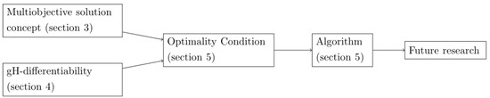
Figure 3.
Sequencing of contents.
2. Preliminaries
We recall the arithmetic and order for intervals we are going to use.
We denote by the family of all bounded closed intervals in , i.e.,
.
For , and , we consider the following operations:
This difference (2), called generalized Hukuhara difference ( difference for short), has many interesting properties compared to other definitions (Minskowki, Hukuhara differences) for example . In addition, the -difference of two intervals and always exists, and it is equal to [24]
Given two intervals, we define the distance between A and B by It is well-known that is a complete metric space.
We consider the following order relation in .
Definition 1.
Let . It is said that
- and , with a strict inequality.
It is clear that .
A fuzzy set on is a mapping . For each fuzzy set , we denote its -level set as | for any . The support of is denoted by where |. The closure of is defined by the 0-level of u, i.e., , where means the closure of the subset . The core of , , is defined by .
Definition 2.
A fuzzy set on , is said to be a fuzzy interval or fuzzy number if the following properties are satisfied:
- 1.
- is normal, i.e., there exists such that ;
- 2.
- is an upper semi-continuous function;
- 3.
- ;
- 4.
- is compact.
Let denote the family of all fuzzy intervals on . Thus, for any , we have that for all , and we denote its -levels by , for all . A fuzzy interval is completely determined by satisfying certain conditions, [17].
Triangular fuzzy numbers are a special type of fuzzy numbers which are well determined by three real numbers . We write to denote the triangular fuzzy number with core or 1-level given by the singleton and whose -levels sets are
for all . A particular case of triangular fuzzy number (or fuzzy number) are the real numbers with a membership function given by , where denotes the characteristic function of the set A. In addition, considering the characteristic function, we can see that any interval is a fuzzy interval, i.e., is a fuzzy interval (fuzzy number) such that , for all .
For fuzzy numbers, , represented by and respectively, and, for any real number , we define the addition and scalar multiplication as follows:
It is well known that, for every ,
Definition 3
([25]). Given two fuzzy intervals and the generalized Hukuhara difference (-difference for short) is the fuzzy interval , if it exists, such that
It is easy to show that and are both valid if and only if w is a crisp number. Note that the case (i) coincides with Hukuhara difference (see [26]), and so the -difference concept is more general than the H-difference one.
If exists, then, in terms of -level sets, we have that
for all , where denotes the gH-difference between two intervals (see [25]).
Given the distance between and is defined by
Thus, is a metric space.
Let us now consider the set of all vector fuzzy intervals, , i.e., if , where each . For any , we have that
Geometrically, it would be a Cartesian product of closed intervals in
Lemma 1.
It is verified that , for all , .
Proof.
If , then , for all and then . □
We recall the usual order for fuzzy intervals based on -level sets:
Definition 4.
For , it is said that:
- , if for every , .If , , then .
- if and , such that .
- if , .
For if either or , then it is said that and are comparable; otherwise, they are incomparable.
Note that is a partial order relation on . Thus, instead of can be written. We observe that, if , then and then .
Henceforth, S denotes an open subset of . Let us consider a fuzzy function or fuzzy mapping. For each , we associate with the interval-valued functions family given by . For any , we denote
Here, for each , the real-valued endpoint functions are called lower and upper functions of , respectively.
3. Multiobjective Problem with Fuzzy Objective Functions
In this paper, we consider the following multiobjective fuzzy mathematical programming problem:
where , are fuzzy functions defined on S, an open non-empty subset in .
Interpreting the meaning of ”minimize a vector fuzzy function,” we give a similar solution concept to the non-dominated solution than the one introduced by Pareto, and usually considered in real-valued multiobjective optimization.
Definition 5.
Let be a vector fuzzy function defined on S. It is said that is an efficient solution or Pareto solution if there exists no such that , and such that .
Notice that the aforementioned definition coincides with the classic one when the functions are real-valued.
In [10], a defuzzification function, and two order relations are defined
Definition 6.
Let and be fuzzy numbers. We write
- if the Hukuhara difference exists and .
- if the Hukuhara difference exists and is nonnegative, where a fuzzy number is said to be nonnegative if for all .
Notice that these definitions can only be applied to fuzzy numbers such that their Hukuhara difference exists, i.e., , , where is the interval range.
Now, we are going to relate those order relations on with the one we propose to use “”:
Proposition 1.
and coincide when Hukuhara difference does exist.
Proof.
If , if and only if because
If , then and . Thus, and reciprocally.
In particular, if the Hukuhara difference does exist, then . If is nonnegative for all . From (5), , therefore and from Definition 4. □
In [23], it is shown that a minimum based on average index ordering relation is a minimum for -level sets ordering relation when , where Y is a subset of the unit interval and P a probability distribution function on Y. In general:
Proposition 2.
If when is a nonnegative fuzzy number, then is equivalent to .
Proof.
Let us suppose that exists, then ⇔⇔⇔ is nonnegative ⇔ forall ⇔. □
Definition 7.
An interval approximation of a fuzzy number is an operator such that, for ,
- (i)
- ,
- (ii)
- ,
- (iii)
- .
Proposition 3
([12]). The interval
is an Interval Approximation of fuzzy number such that minimizes for all I belonging to the space of interval approximation operators of fuzzy numbers. is called Nearest Interval Approximation (NIA).
Notice that is the distance between fuzzy numbers, defined in , and it can be considered here since each interval is also a fuzzy number with constant -level sets for all .
In [13] to find a solution of , the authors have approximated it by the following interval multiobjective program:
where stands for the nearest interval approximation (NIA) of , i.e., , that it is among the interval approximation operators of a fuzzy number, the one that minimizes the distance to the fuzzy number.
Definition 8
([13]). is called a satisficing solution of (P) if it is a Pareto optimal solution of (P1), i.e., if there is no such that for all and .
Proposition 4.
If is a satisficing solution of , then is a Pareto solution for .
Proof.
Let us suppose that there exists such that . Then, it follows that and , and thus and besides there exists k such that and , and thus . It stands in contradiction to the hypothesis. □
In this way, it is demonstrated that the Pareto solution concept used in this work includes as particular cases those existing in the literature.
4. gH-Differentiable Fuzzy Functions
In Optimization Theory, when the functions are differentiable, their gradients allow us to find analytical optimality conditions. Different fuzzy differentiability concepts have been used in fuzzy optimization (H-differentiability, G-differentiability, level-wise differentiability), but they are more restrictive than the -differentiability [27,28,29].
Next, we present the -differentiable fuzzy function concept based on the -difference of fuzzy numbers.
Definition 9
([30]). The -derivative of a fuzzy function at is defined as
If satisfying (6) exists, we say that is generalized Hukuhara differentiable (-differentiable, for short) at .
The following results establish relationships between gH-differentiability of and the gH-differentiability of the interval-valued functions family , and the differentiability of its endpoint functions and .
Notation 1.
For simplicity, we use the following notation for an interval. If are the end-points of the interval (but it is not necessarily ), we write .
Theorem 1
([31]). If is -differentiable at , then is -differentiable at uniformly in and
for all .
From Theorem 1 and using Theorem 8 given by Qiu [32], it is verified that
Theorem 2.
Let be a fuzzy function. If is -differentiable at , then the lateral derivatives of real-valued endpoints functions , , and exist, uniformly in , and satisfy
Remark 1.
As a consequence of the aforementioned results, we use the following notation:
where
Definition 10.
Given a fuzzy vector function , we say that is a vector -differentiable fuzzy function at if and only if is -differentiable at , for all .
5. Necessary Conditions for Pareto Solutions
In this section, we prove a necessary optimality condition for Pareto solutions and give an algorithm based on it, in order to find all the potential candidates to be optimum for our problem. With the necessary optimality conditions, we can exclude feasible solutions that are not optimums. In Section 3, we have proved that optimum concepts used until now in the different strategies to solve a fuzzy multiobjective programming problem are more restrictive than the Pareto solution concept based on the -level sets. Thus, the algorithm we develop here remains valid for the other optimum notions.
In [16], the same Pareto efficiency notion we propose in this paper is used, and a sufficient optimality conditions for it is proved, but using more restrictive hypotheses on the functions (level-wise differentiable functions) than the ones we suppose here. Thus, the necessary optimality condition presented here and the algorithm developed remain valid in the context of that paper [16].
Notation 2.
For convenience, we introduce the following notations. Let be with . Letting , we denote by the lineal combination
If for some , then there exists , and not all zero, such that: .
If with , but not all zero, there exist , such that
with and .
Proposition 5.
Let be a vector -differentiable fuzzy function on S. If is an efficient or Pareto solution for , then the following system does not have a solution at :
Proof.
Arguing by contradiction, let us suppose that such that
Then,
From Theorem 2, for each j, there exist and , uniformly in , and they satisfy
Since
From
Thus, it follows that there exist , such that, for all t, with
In addition, analogously there exists such that, for all t, with
Now, we prove the main result of this section.
Theorem 3.
Let be a vector -differentiable fuzzy function at . If is an efficient or Pareto solution for , then there exists a non-negative matrix such that
Proof.
Now, let us consider the following lineal system and let us prove it has no solution:
where and
If (11) has a solution, then the system (7) also would have a solution, and this is impossible by Proposition 5.
Since (11) is a system of linear inequalities and it does not have solution, from Gordan’s alternative theorem, there exist with , but not all zero, such that
Redefining , we obtain that there exists such that
In addition, the proof is completed. □
Remark 2.
If there exists such that , (12) is verified, and then, to identify possible candidates for Pareto solutions, is reduced to identify those feasible solutions whose 0-level set of the derivative contains the zero element. This coincides with the result for a unique objective function given by Osuna-Gómez et al. [23].
Remark 3.
From Theorems 2, 3 and Remark 3, an algorithm to identify the Pareto solutions candidates can be designed, in the same form as in classical Mathematical Programming. We solve the equations where the gradients are equal to zero in order to identify the possible optima.
The corresponding flow chart is (Figure 4):
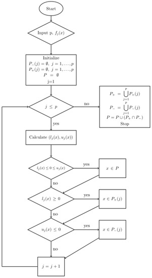
Figure 4.
Flow chart.
The algorithm can be described as:
- Step 1. Start and input p (Objective function )
- Step 2. Put , , ,
- Step 3. While
- Step 3.1 .
- Step 3.2 Calculate
- Step 3.3 Define and find ,
- Step 3.4 Put
- Step 3.5 For x such that , then .
- Step 3.6 For x such that , then
- Step 3.7 For x such that , then
- Step 3.8
- Step 4. Set and . If then
- Step 5. Print P = possible Pareto solutions set and stop.
Example 1.
We look for the Pareto optimal solutions for
- In step 1, let us consider two fuzzy functions , whose α-level sets are given by, respectively, because , where C is a fuzzy interval.
- In step 2, for , we begin with , and .
- In step 3, for , .Then, , so we get that is a possible Pareto efficient solution for , andFor , and so and
- In Step 4, and
- In step 5, in summary, we get that is a possible Pareto efficient solution for . It is represented in the following Figure 5:
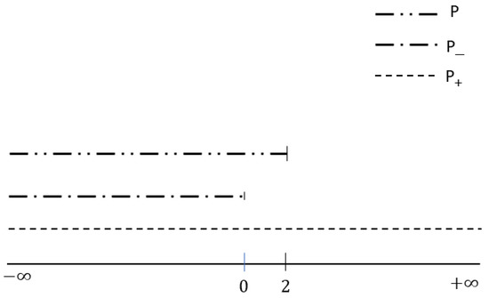 Figure 5. Pareto solutions set.
6. Conclusions
In this paper, we have addressed the resolution of a fuzzy multiobjective programming problem using the -level sets optimization. We have obtained a necessary condition for Pareto-type solutions from the -level sets and have provided an algorithm and an example based on it.
The advantages of our method are focused on: the solution concept used, based on the -level sets, encompassing those previously presented in the literature; the algorithm proposed, that locates the optimal candidates easily and comfortably; the generalization to multiobjective fuzzy case of results obtained for fuzzy scalar problems and real-valued multiobjective problems.
The disadvantages or limitations are the necessity of gH-differentiability for the involved functions, and the proposed algorithm does not allow for identifying the points that are not solutions.
In our opinion, future work should be based, on the one hand, on obtaining sufficient conditions that can identify optimal solutions to multiobjective problems, not only candidates for optimal solutions and that are generalizable to control and variational problems. On the other hand, future work should focus on exploring more complete algorithms (such as the bisection search method, Newton’s method, the cyclic coordinate method, Rosenbrock’s method, and others) based on the obtained optimality conditions that allow for the effective and practical search of the solutions.
Author Contributions
Writing—review and editing, B.H.-J., G.R.-G., A.B.-M. and R.O.-G. All authors have read and agreed to the published version of the manuscript.
Funding
This research received no external funding.
Acknowledgments
The authors would like to thank the referees for their suggestions that have improved the initial manuscript and the Institute for Social and Sustainable Development (INDESS) for the facilities provided for the preparation of this article.
Conflicts of Interest
The authors declare no conflict of interest.
References
- Zimmerman, H.J. Fuzzy programming and linear programming with several objective functions. Fuzzy Sets Syst. 1978, 1, 45–55. [Google Scholar] [CrossRef]
- Hu, Y.; Zhang, Y.; Gong, D.W. Multiobjective Particle Swarm Optimization for Feature Selection With Fuzzy Cost. IEEE Trans. Cybern. 2021, 51, 874–888. [Google Scholar] [CrossRef] [PubMed]
- Jamwal, P.K.; Hussain, S. A fuzzy based multiobjective optimization of multi echelon supply chain network. J. Intell. Fuzzy Syst. 2020, 39, 3057–3066. [Google Scholar] [CrossRef]
- Milenkovic, M.; Bojović, N. Fuzzy multiobjective rail freight car fleet composition. In Optimization Models for Rail Car Fleet Management; Elsevier, 2020; Available online: https://www.sciencedirect.com/book/9780128151549/optimization-models-for-rail-car-fleet-management (accessed on 25 March 2021).
- Goli, A.; Zare, H.K.; Tavakkoli-Moghaddam, R.; Sadegheih, A. Multiobjective fuzzy mathematical model for a financially constrained closed-loop supply chain with labor employment. Comput. Intell. 2020, 36, 4–34. [Google Scholar] [CrossRef]
- Sun, Y. A Fuzzy Multi-Objective Routing Model for Managing Hazardous Materials Door-to-Door Transportation in the Road-Rail Multimodal Network With Uncertain Demand and Improved Service Level. IEEE Access 2020, 8, 172808–172828. [Google Scholar] [CrossRef]
- Birjandi, M.R.S.; Shahraki, F.; Razzaghi, K. Hydrogen and CO2 Management in the Refinery with Fuzzy Multiobjective Nonlinear Programming. Chem. Eng. Technol. 2019, 42, 1941–1951. [Google Scholar] [CrossRef]
- Bigdeli, H.; Hassanpour, H.; Tayyebi, J. Multiobjective security game with fuzzy payoffs. Iran. J. Fuzzy Syst. 2019, 16, 89–101. [Google Scholar]
- Upmanyu, M.; Saxena, R.R. On solving multi objective Set Covering Problem with imprecise linear fractional objectives. RAIRO-Oper. Res. 2015, 49, 495–510. [Google Scholar] [CrossRef]
- Wu, H.C. Solutions of fuzzy multiobjective programming problems based on the concept of scalarization. J. Optim. Theory Appl. 2008, 139, 361–378. [Google Scholar] [CrossRef]
- Wu, H.C. Using the technique of scalarization to solve the multiobjective programming problems with fuzzy coefficients. Math. Comput. Model. 2008, 48, 232–248. [Google Scholar] [CrossRef]
- Grzegorzewski, P. Nearest interval approximation of a fuzzy number. Fuzzy Sets Syst. 2002, 130, 321–330. [Google Scholar] [CrossRef]
- Luhandjula, M.K.; Rangoaga, M.J. An approach for solving a fuzzy multiobjetive programming problem. Eur. J. Oper. Res. 2014, 232, 249–255. [Google Scholar] [CrossRef]
- Ren, A.; Wang, Y. An approach for solving a fuzzy bilevel programming problem through nearest interval approximation approach and KKT optimality conditions. Soft Comput. 2017, 21, 5515–5526. [Google Scholar] [CrossRef]
- Sharma, U.; Aggarwal, S. Solving fully fuzzy multi-objective linear programming problem using nearest interval approximation of fuzzy number and interval programming. Int. J. Fuzzy Syst. 2018, 20, 488–499. [Google Scholar] [CrossRef]
- Wu, H.C. The optimality conditions for optimization problems with convex constraints and multiple fuzzy-valued objective functions. Fuzzy Optim. Decis. Mak. 2009, 9, 295–321. [Google Scholar] [CrossRef]
- Goestschel, R.; Voxman, W. Elementary fuzzy calculus. Fuzzy Sets Syst. 1986, 18, 31–43. [Google Scholar] [CrossRef]
- Ruiz-Garzón, G.; Osuna-Gómez, R.; Rufián-Lizana, A.; Hernández-Jiménez, B. Optimality and duality on Riemannian manifolds. Taiwan J. Math. 2018, 22, 1245–1259. [Google Scholar] [CrossRef]
- Ruiz-Garzón, G.; Osuna-Gómez, R.; Ruiz-Zapatero, J. Necessary and sufficient optimality conditions for vector equilibrium problems on Hadamard manifolds. Symmetry 2019, 11, 1037. [Google Scholar] [CrossRef]
- Ruiz-Garzón, G.; Ruiz-Zapatero, J.; Osuna-Gómez, R.; Rufián-Lizana, A. Neccesary and sufficient second-order optimality conditions on Hadamard manifolds. Mathematics 2020, 8, 1152. [Google Scholar] [CrossRef]
- Ruiz-Garzón, G.; Osuna-Gómez, R.; Rufián-Lizana, A.; Hernández-Jiménez, B. Approximate efficient solutions of the vector optimization problem on Hadamard manifolds via vector variational inequalities. Mathematics 2020, 8, 2196. [Google Scholar] [CrossRef]
- Treanta, S.; Arana-Jiménez, M.; Antczak, T. A necessary and sufficient condition on the equivalence between local and global optimal solutions in variational control problems. Nonlinear Anal. 2020, 191, 111640. [Google Scholar] [CrossRef]
- Osuna-Gómez, R.; Hernández-Jiménez, B.; Chalco-Cano, Y.; Ruiz-Garzón, G. Different optimum notions for fuzzy functions and optimality conditions associated. Fuzzy Optim. Decis. Mak. 2018, 17, 177–193. [Google Scholar] [CrossRef]
- Stefanini, L.; Bede, B. Generalized Hukuhara differentiability of interval-valued functions and interval differential equations. Nonlinear Anal. 2009, 71, 1311–1328. [Google Scholar] [CrossRef]
- Stefanini, L. A generalization of Hukuhara difference and division for interval and fuzzy arithmetic. Fuzzy Sets Syst. 2010, 161, 1564–1584. [Google Scholar] [CrossRef]
- Hukuhara, M. Integration des applications mesurables dont la valeur est un compact convexe. Funkc. Ekvacioj 1967, 10, 205–223. [Google Scholar]
- Stefanini, L.; Arana-Jiménez, M. On Fréchet and Gateaux derivatives for interval and fuzzy-valued functions in the setting of gH-differenciability. In Proceedings of the 2020 IEEE International Conference on Fuzzy Systems (FUZZ-IEEE), Glasgow, UK, 19–24 July 2020; pp. 1–6. [Google Scholar]
- Puri, M.L.; Ralescu, D.A. Differentials for fuzzy functions. J. Math. Anal. Appl. 1983, 91, 552–558. [Google Scholar] [CrossRef]
- Bede, B.; Gal, S.G. Generalizations of the differentiability of fuzzy number valued functions with applications to fuzzy differential equation. Fuzzy Sets Syst. 2005, 151, 581–599. [Google Scholar] [CrossRef]
- Bede, B.; Stefanini, L. Generalized differentiability of fuzzy-valued functions. Fuzzy Sets Syst. 2013, 230, 119–141. [Google Scholar] [CrossRef]
- Chalco-Cano, Y.; Rodríguez-López, R.; Jiménez-Gamero, M.D. Characterizations of generalized differentiable fuzzy functions. Fuzzy Sets Syst. 2016, 295, 37–56. [Google Scholar] [CrossRef]
- Qiu, D. The generalized Hukuhara differentiability of interval-valued function is not fully equivalent to the one-sided differentiability of its endpoint functions. Fuzzy Sets Syst. 2020. [Google Scholar] [CrossRef]


Publisher’s Note: MDPI stays neutral with regard to jurisdictional claims in published maps and institutional affiliations. |
© 2021 by the authors. Licensee MDPI, Basel, Switzerland. This article is an open access article distributed under the terms and conditions of the Creative Commons Attribution (CC BY) license (https://creativecommons.org/licenses/by/4.0/).