Detailed Study on the Behavior of Improved Beam T-Junctions Modeling for the Characterization of Tubular Structures, Based on Artificial Neural Networks Trained with Finite Element Models

Abstract

The actual behavior of welded T-junctions in tubular structures depends strongly on the topology of the junction at the joint level. In finite element analysis, beam-type elements are usually employed due to their simplicity and low computational cost, even though they cannot reproduce the joints topologies and characteristics. To adjust their behavior to a more realistic situation, elastic elements can be introduced at the joint level, whose characteristics must be determined through costly validations. This paper studies the optimization and implementation of the validation data, through the creation of an optimal surrogate model based on neural networks, leading to a model that predicts the stiffness of elastic elements, introduced at the joint level based on available data. The paper focuses on how the neural network should be chosen, when training data is very limited and, more importantly, which of the available data should be used for training and which for verification. The methodology used is based on a Monte Carlo analysis that allows an exhaustive study of both the network parameters and the distribution and choice of the limited data in the training set to optimize its performance. The results obtained indicate that the use of neural networks without a careful methodology in this type of problems could lead to inaccurate results. It is also shown that a conscientious choice of training data, among the data available in the problem of choice of elastic parameters for T-junctions in finite elements, is fundamental to achieve functional surrogate models.

1. Introduction

The utilization of finite element modeling for the simulation of structural components has become a fundamental part of modern engineering, being utilized in the majority of industrial fields.

Despite the advances of the finite element analysis (FEA) software and the increased calculation capabilities, for the modeling of tubular structures in which the length of the profiles is significantly bigger than the width and thickness of the sections, the beam type elements are still widely utilized despite their limitations and the fact that they cannot reproduce the characteristics of the joints neither from the geometrical point of view nor from the behavioral one. Figure 1 presents the equivalent beam type element T-junction that would be utilized for the simulation of the original T1 and T2 junctions.

The joint configuration of these T-junctions (T1 and T2) has a direct influence on the behavior of the structures, determining significant behavioral differences depending on the type and direction of the load. Despite this reality, the beam type element equivalent model will always be composed of three nodes and three beam type elements. This way all the geometrical characteristics of the joint get lost into an infinitely rigid node, which represents a significant shortcoming of these elements in the correct characterization of T-junctions.

This issue could be avoided by utilizing shell or volume type elements. However, these alternatives are feasible only for small models, which is not the case when common tubular structures such as buses upper modules, bridges, support structures, or similar big structures need to be modeled. The complexities of the modeling process along with the increase in computational resources due to the increment of nodes make these alternatives unfeasible for general industrial use.

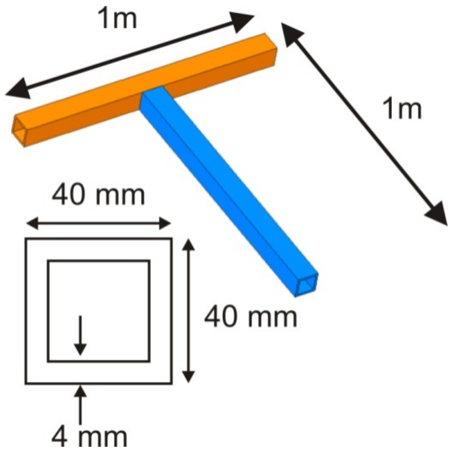
The magnitude of this issue is illustrated in

Table 1. Comparative analysis between characteristics of T-junctions modeled with beam, shell, and volume type elements.

Element Type	No. of Nodes	DOFs	Complexity of Modeling (1–3)	Results Precision (1–3)	Evaluation Coefficient
Beam	910	5460	1	3	16,380
Shell	19,520	117,120	2	2	468,480
Volume	36,144	108,432	3	1	325,296

, in which a comparative analysis is performed based on the number of nodes and degrees of freedom for a simple T-junction of 1 m by 1 m having a standard square hollow profile of 40 mm × 40 mm × 4 mm presented in Figure 2. The table presents the comparative analysis of the T-junction, modeled using beam, shell and volume element types, for comparative purposes, the three models where meshed using 4 mm first order elements. The resulting number of nodes are a consequence of the meshing dimension and the degrees of freedom are calculated taking into consideration the mathematical formulation of the elements. In the case of the beam and shell elements we have 6 degrees of freedom (DOF) per node and in the case of the volume type elements we have 3 DOF per node. A comparative evaluation criterion taking into consideration the complexity of the modeling process and the precision of the results, based on the experience of the authors for modeling structures. The value is calculated as the product between the DOFs and the complexity of the modeling process along with the precision of the results (Table 1).

From the previously presented results, it can be seen that, despite their limitations, the beam type elements represent the most feasible alternative when analyzing tubular structures in which the relation of the length and the profile dimensions is quite significant. Due to the above, it can be concluded that the calculation of complex tubular structure (buses, bridges, and railway carriages) is significantly simplified by using beam-type elements. This is why, these elements have been widely recommended [1,2,3] for modeling large tubular structures.

However, despite being recommended and widely utilized in the industry, the beam formulation is simply not designed to take into account and reproduce the behavior of real joints, since all the elements that reach the same joint are joined in a single infinitely rigid node [4,5,6]. Furthermore, beam-type elements cannot represent the topological characteristics of the joints and do not differentiate between joints that are apparently similar, but with different topologies. Therefore, there is a clear necessity for the improvements of the beam modeled T-junctions.

One of the improvement solutions proposed in order to avoid ignoring the specific characteristics of the joint topologies was the introduction of elastic elements at the joint level when modeling T-junctions. In [4] it was shown that the flexibility of the joints has a determining influence on the behavior of the analyzed structures and could not be ignored. Later, in [5] it was again confirmed that ignoring the influence of joint stiffness on structural behavior was a mistake. In this case, it was shown that, when the stiffness of the elastic elements in the joint exceeds a certain maximum value, the total deformation energy of the vehicle is insensitive to the joint.

Furthermore, in [7], Lee presented the hypothesis that the behavior of welded joints was elastic and linear, obtaining a general methodology for the model of joints. Applying this, in [8], three rotational springs were introduced into the joints with the aim of optimizing vehicle structures. This way, the deformations that could occur in the joints due to torsional or bending moments were considered. In contrast, infinite stiffness values were assumed in the axial directions, this study showed that it was possible to obtain better approximations with this approach and validated modal calculations with experimental modal analyses. The introduction of elastic elements when modeling beam T-junctions has a fundamental advantage since it provides the possibility to modify the overall behavior of the structure while maintaining the mass distribution of the input model, having the downside of requiring the adjustment of the appropriate stiffness values which would lead to the need for expensive experiments.

Another alternative was to model beam T-junctions with variable stiffness in the adjacent regions to the joints, this was proposed in [9] since the rigidity of the joint is much greater than the surrounding area. Later, in [10] the idea was reformulated by using partially rigid beams. Taking advantage of this new concept, in [11] H-shaped structures with rectangular hollow profiles were studied and partially rigid beams were used at their joints, the model was validated through modal correlation with good results. The same methodology was applied in [12] for the optimization of a three-dimensional bus structure formed by hollow rectangular profiles of 40 mm × 40 mm × 3 mm. To do this, it was necessary to perform a sensitivity analysis to identify the joints that had the greatest influence on the overall behavior of the structure, this way, partially rigid beams were progressively introduced in the most important regions. Alternatively, a new technique was proposed in [13]. In this case, the parameters of the elements near the joint were modified. This approach of the problem is similar to the previous one, but also allowing the modification of the mass and rigidity independently.

Given these limitations, some authors have used shell or volume type elements as an alternative for the study of the joints, modeling the rest of the structure with beam type elements, these elements allow the characteristics of the joint to be modeled more accurately. In [14] the shell element model was applied to tubular joints and major improvements were reported. In [15] the models of a single beam with shell elements were compared against the same shell and beam modeled and it was shown that hybrid modeling could reduce the number of elements without compromising the results.

The same approach has been applied to the analysis of structural joints in cars. Thus, hybrid modeling has led to satisfactory results [14,16,17] in this field, however, the application of this hybrid technique to larger models (e.g., hollow beam structures in buses) is unattractive, since it would be necessary to specifically model a large number of joints, which leads to a substantial increase in the model preparation time and more computational resources by increasing the number of elements in the model.

In their study [18] developed an alternative beam T-junction model that allowed them to obtain more precise deformation results when utilizing beam type elements, also allowing them to take into consideration different T-junction configurations. Their focus was to improve the results provided by beam type elements when simulating structures that by their characteristics cannot be realistically simulated with anything but beam type elements due to the complexity of the modeling process, the computational requirements or other practical aspects. The authors proposed an alternative beam model in which they introduced a total of six elastic elements at the joint level along with a complete methodology based on finite element methodology (FEM) comparative analysis that allowed them to improve the behavior of the modeled T-junctions in terms of displacements. This proposal, however, required the user to reproduce the complete methodology in order to obtain six stiffness values for each individual modeled T-junction making it somehow not attractive when having to characterize a wide variety of T-junction combinations. Figure 3 presents the alternative beam T-junction model proposed and utilized by [18]. This T-junction introduces a total of six elastic elements at the joint level, three of them behaving as linear springs (represented by the letter k) and noted with the sub index ux, uy, and uz corresponding to (u) displacement and (x, y, z) the axial directions and another three corresponding to (r) rotations along the (x, y, z) axial directions.

This approach was also used by [19], in which multiple simulations utilizing the most common profiles found in buses and coaches upper structures were performed, followed by a statistical analysis in order to obtain regression models for the calculation of the stiffness values for the alternative T-junctions, based on the profile dimensions (E1, E2, E3, g1, and g2). They utilized a Bayesian Kriging regression model that provided satisfactory results, however, the regression equations obtained were notably complicated having, in some cases, more than 33 terms per equation, making them impractical for everyday use in the wide industry. These regressions were obtained with a MISO (multiple input, single output) approach in which a total of six regression models had to be calculated, one for each k_ux, k_uy, k_ux, k_rx, k_ry, and k_rz stiffness value, leading to the necessity of any potential user to use six complex equations for the estimation of the stiffness values for a single T-junction type.

From the previous studies it can be concluded that it is possible to make an adjustment of the existing data coming from analysis by finite elements in complicated models. In this way, the time and effort needed to carry out new simulations for sets of junction parameters not previously studied can be drastically reduced. Unfortunately, the basic laws that allow for optimal adjustment are not known. In this sense, artificial neural networks (ANN) surrogate models allow, from sufficient known training data, to infer the unknown laws behind the analyzed data. The use of ANNs is not new. There are countless studies that have applied them to the most diverse applications. Specifically, in the last years, the development and implementation of neural networks for the evaluation of multiple processes with a pronounced non-linear behavior has become a reality [20]. ANN have also been utilized along with finite elements such as in [21] where the authors implemented their use with good results in the evaluation of damage detection in bridges. In [22], ANN was used to simplify contact estimation models in ANSYS^®. In [23] the use of response surface and ANN models was successfully evaluated against other methods of structural reliability analysis. In addition, ANNs can generate valid surrogated models, based on data obtained from finite elements, to evaluate such complicated issues as noise reduction in braking systems, with very high accuracy [24].

Taking into consideration the benefits of the implementation of neural networks for finite element analysis, the authors considered of great interest the development of a methodology for the estimation of the stiffness values utilizing ANN as an alternative to the utilization of Bayesian Kriging regressions similar to those utilized in [19], that provided satisfactory results although not realistic from the practical point of view due to the complexity of the obtained equations. In fact, ANNs have been used as a valid alternative to such Kriging networks in various articles for the creation of metamodels [25,26] providing very satisfactory results.

This article studies the application of ANN in the creation of surrogate models that allow inferring the information obtained from complicated finite element models, such as those obtained in the analysis of optimal stiffness to predict the behavior of T-welded junctions. The biggest problem when trying to replace finite element modeling with surrogate models is that a lot of training data needs to be obtained for the prediction to be reliable. However, obtaining this data is often very costly in time and effort. There is also uncertainty about how the ANN should be created to learn effectively and be useful for unknown finite element models.

This article presents a detailed study, leading to the presentation of a new methodology for the creation of surrogate models (or metamodels) based on data obtained from finite element calculations. The particularity in this case is that the number of initial data, for the training of the model, is very limited. Few training data can make the model a failure. However, as mentioned, this is usually a common situation in FEM due to the high time of creation of FEM models and their calculation. The possibility of creating models that can learn from these “few” data obtained from FEM calculations, using them in an optimal way, can allow to obtain more precise models and enable the use of ANN to cases with limited data.

The rest of the article is distributed as follows: Section 2 presents the methodology followed for the determination of the ANN topology and the optimal use of the available data; Section 3 describes the results and the analyses obtained, which are discussed in Section 4. Finally, Section 5 presents the conclusions, applicability, and future lines.

2. Methodology

Using the same data from [19] the experimental design for the neural network analysis had a five dimensional input and six dimensional output, where the input values represented the dimensions of the analyzed T-junction profiles (E1, E2, E3, g1, and g2) and the output values represented the calculated stiffness values for the alternative T-junction model having 3 axial spring (k_ux, k_uy, k_uz) and 3 rotational springs (k_rx, k_ry, k_rz) at the junction level as presented in Figure 3.

This data is based on hollow rectangular profiles commonly utilized in the buses and coaches upper structures, focusing the study on a total of 243 profile combinations for two different T-junction configurations named T1 and T2 presented in Figure 1.

The 243 input values were obtained by getting all of the possible combinations for the five input variables, each variable having 3 levels as presented in

Table 2. Input base variable values.

E1 (mm)	E2 (mm)	E3 (mm)	g1 (mm)	g2 (mm)
40	40	40	2	2
60	60	60	3	3
80	80	80	4	4

.

As can be seen in the previous table, the input data is staggered and only provides information about the studied process for specific values, leaving significant empty spaces between variables as can be seen in Figure 4, in which the utilized input values for the E1–E3 characteristics are plotted in a 3D graphic.

Since the base methodology requires comparative FEM analysis between beam and shell modeled T-junctions, for example adding 2 additional thicknesses for the g1 and g2 variables, would require a total of 675 comparative simulations for each one of the T1 and T2 junctions determining a significant increase in the required computational time. This leads to a situation in which predictive models need to be constructed from a limited amount of staggered input data, in which a proper selection of the neural network training data is of paramount importance. 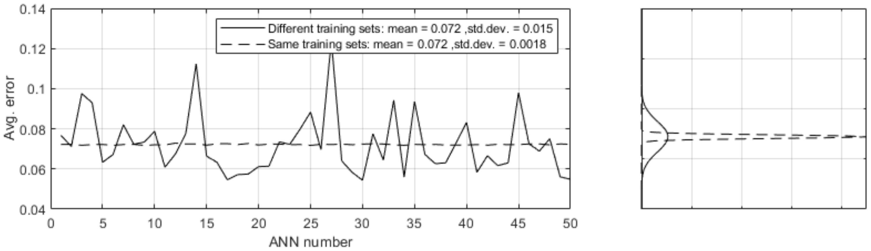To illustrate that, Figure 5 presents the average error obtained for 50 different neural networks, constructed using different training data sets versus using the same training data set. This error is determined for each neural network as the average difference between the network output values and the target outputs of the validation data obtained from FEM models. As it can be seen, although both cases reach the same average error (0.072), the standard deviation is almost one order of magnitude higher in the case of neural networks constructed using different training data, evidencing the importance of a proper selection of this data.

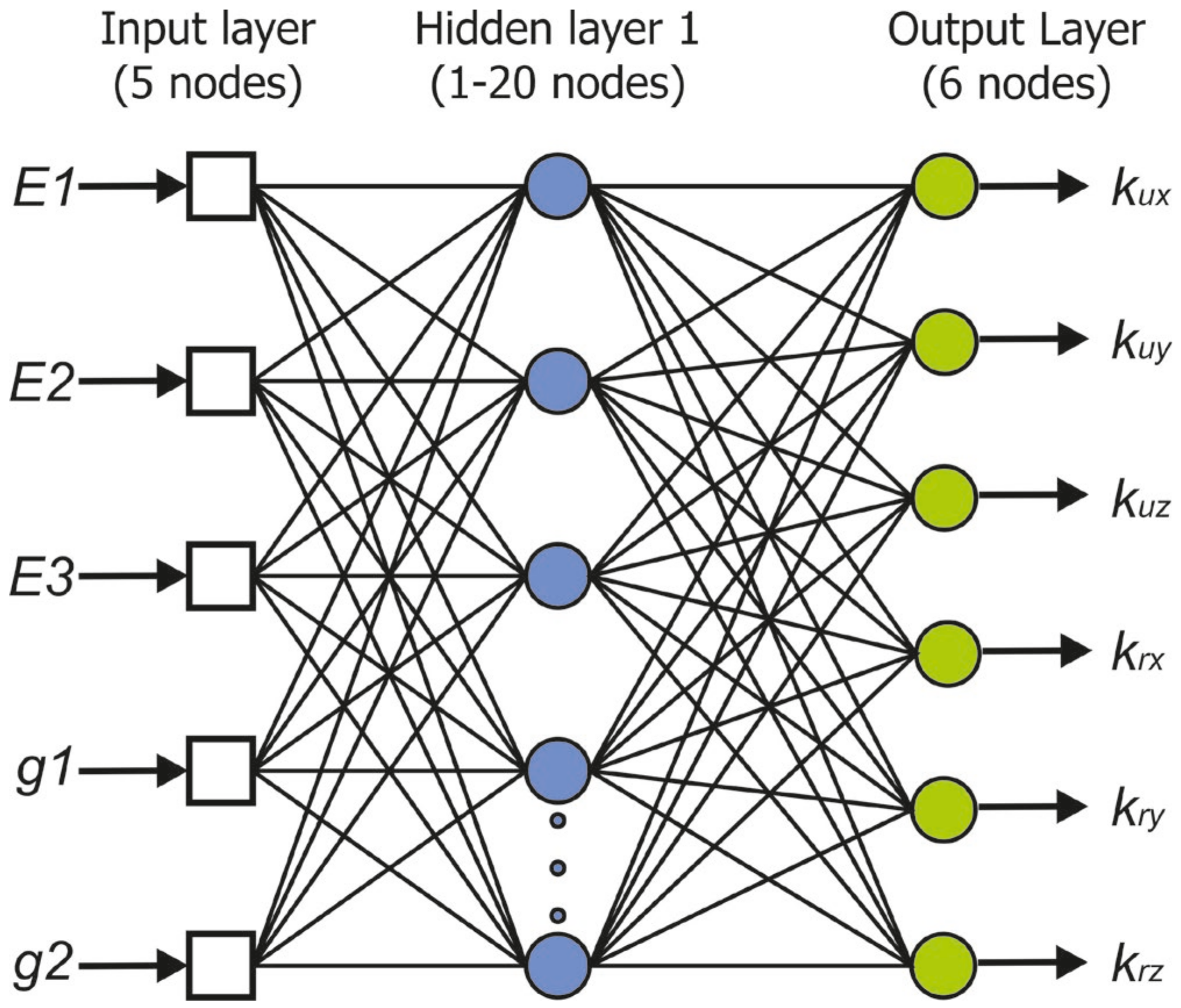
This behavior motivates a more detailed study of the performance of neural networks with respect of the chosen data set. To carry out this study it was necessary to decide the topology and design of a neural network that could be effectively trained from few input data. In a neural network, the increase of hidden layers and nodes in each layer, requires a lot of training data to avoid the known problem of over fitting. As the number of training data is very limited in our case the network was kept simple, with only one hidden layer and a limited number of nodes (1 to 20) within that layer. In addition, to check the performance of the neural network, the initial data were divided into two subsets. The first one was dedicated to the training of the network (75% of them) and the second one to its validation (25%). Usually, the distribution of training and validation data is around 50% in cases where there are large amounts of data. However, in this case, due to the high cost of obtaining additional training data, it was decided to vary the standard. The rest of the parameters and functionality of the neural network were also kept simple. For the comparison between the outcome between neural networks a limit of 2000 training iterations (epocs) was taken, with a learning rate of 0.1. The activation function of the neurons was the hyperbolic tangent sigmoid, and the training was based on a Levenberg–Marquardt backpropagation algorithm, Figure 6 presents the characteristics of the ANN.

As mentioned, the limitation of training data has a fundamental influence on the choice of the type of neural network to be used, its topology and its configuration, since it can cause the network not to learn the pattern behind the data, or to learn it too well, fitting perfectly to the training data, but offering very poor results in the validation data. This effect is called over fitting and it is critical to avoid it. The goal is to train with as much data as possible and to learn in a robust way and to reduce the error in the validation data.

But, apart from the issue of reasoned choice of network topology, there is the major problem of optimal selection of training data. Since there is so little training data, the information that such data provides about the behavior of the welded T-joints is very valuable. The choice of which data should be used for network training and which data should be used for validation has a critical influence on the result of the analysis. Therefore, the choice of which data will go to 75% of the training set should not be made at random in this type of problem. At this point, the choice of suitable training sets is not evident. For this reason, a thorough study is needed to shed light on this point.

In this sense, next sections show the results of this complete study, where a total of 1000 different training data sets were used to construct the neural network, leading to a total of 20,000 different neural networks for each joint configuration. Input layer consisted of 5 neurons containing input information of the joint dimensions (E1, E2, E3, g1, and g2, see Figure 3 and Table 2). For the output layer both MISO (multiple input single output) and MIMO (multiple input multiple output) models were initially explored. Both approaches showed very similar results, so it was decided to focus on MIMO models due to the obvious computational cost saving of not having to construct independent neural networks for each output. Thus, output layer consisted of 6 neurons with the 6 DOF spring rates (k_ux, k_uy, k_uz, k_rx, k_ry, and k_rz, see Figure 3). Due to the different behavior of the different joint configurations, independent neural networks were analyzed for T1 and T2 junctions (Figure 1). 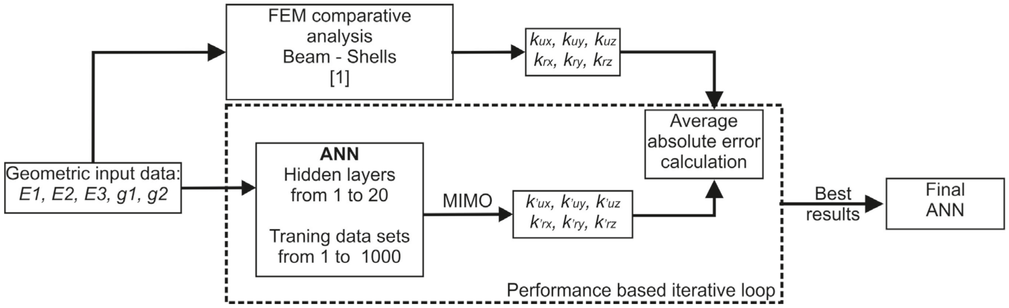The following Figure 7 shows a block diagram with the methodology used to construct and check the performance of each neural network. As it is shown, the same input data with the geometric information that was used to construct the beam and shell FEM models and obtain the spring stiffness, is used to feed the neural networks, which are constructed using 1000 randomly chosen trained sets, and 1 to 20 neurons in its hidden layer. For each network, the average error is recorded, which is obtained as the mean absolute difference between the predicted and correct outputs of the validations set (remaining 25% of the data).

Finally, once the complete methodology is executed, the best performance networks are selected for further analysis in order to validate the selection methodology proposed.

3. Results and Analysis

In the following subsections, the most relevant information, and the obtained results of the application of the methodology will be presented.

3.1. Neural Networks Behavioral Analysis Results

This section shows all relevant findings encountered during the application of the methodology itself. It should be noted that, although of great interest to understand the behavior of the data, the analysis presented in this section in not strictly necessary to run the methodology since it does not affect the network selection, which ultimately depends in the overall average error.

In relation to the performance of the neural network with respect to the number of neurons, Figure 8 shows the average error obtained for each spring and joint configuration, averaged over the 1000 training data sets utilized. As it can be seen, the minimum error values are generally obtained for a number of neurons that ranges approximately between 5 and 10. It can be also noticed that the error level is highly dependent on the spring direction and the junction configuration.

Although in some cases the average error reach minimum values for more than 10 neurons, it was observed that the variability of these errors increased significantly as the number of neurons is increased, and that some outputs with extremely bad predictions where obtained. In this regard, Figure 9 shows the number of networks observed with an average error above one, identified as outliers. It is clearly noticed that from about 10 neurons, outlier results start to increase. In general, springs with better performance show fewer networks with exceptionally high errors.

With respect to the performance of the networks regarding the training data, it was noticed a dependency among the number of neurons, i.e., if any network performs optimally for a given number of neurons, it will show the same tendency for the rest number of neurons. To assess this, the 1000 networks were ranked from 1 (least error) to 1000 (highest error) for each direction and number of neurons. If a given training data shows similar rankings for all number of neurons, it would mean that such dependency of the performance with respect to the number of neurons exists. On the other hand, if the rankings from 1 to 20 neurons approach to a uniform distribution, it would indicate not dependency at all. This behavior was quantified by means of the standard deviation of the rankings in Figure 10, for both junction configuration and spring direction. It is noticed that dispersion of rankings is always significantly lower than the one for uniform distribution (σ = 288.6), and that it is especially low for networks that show best or worst rankings, meaning that dependency is especially high in these cases. As expected, behavior differences are observed between junction configuration and spring direction.

Additionally to the relation of the network performance with respect to the number of neurons, possible dependency with respect to the spring directions were also assessed to check if a given network that performs optimally in one direction, should show the same tendency for the rest of directions. To quantify that in an equivalent manner, standard deviation of the rankings with respect to the spring directions were obtained for each number of neurons, as shown in Figure 11. For the sake of clarity, and since the behavior was found to be very similar for all number of neurons, only results for 1, 5, 10, and 15 neurons are included. In this case, it is observed that for mid rankings, no significant dependency between directions can be stated, since dispersions approaches to the one of uniform distribution. In contrast, extreme rankings show once again lower dispersion, meaning that networks with worst and best results will show dependency between spring directions.

Finally, a detailed analysis of the characteristics of the networks that showed the best results was carried out in order to evaluate if there is any affinity among them regarding the input data and variable values. To do so, the 10 best overall ranked networks were selected for both T1 and T2. Later, the input data that was present in at least 8 out of the 10 for all directions were accounted. These data are highlighted for the 243 input data (abscissa), and for each spring direction (ordinate), for both T1 and T2 in Figure 12 and Figure 13, respectively. It can be noticed that there are certain input data that appears systematically in all best performance networks (14 data inputs are shown for T1 in Figure 12, and 13 data inputs are shown for T2 in Figure 13), regardless the spring directions. It is also noticed that such data are different for T1 and T2 junction configurations.

Furthermore, the values of the geometric variables contained in these input data that appeared systematically in at least 8 out of the 10 best performance networks (14 in Figure 12 and 13 in Figure 13) are analyzed in Figure 14 and Figure 15 for T1 and T2, respectively. The figures show the frequencies of each parameter value. It is noticed a clear tendency to certain values for some of the parameters. Junction configuration T1, for example, takes preferably lower values of E2, and higher values for E3 and g1; meanwhile, junction configuration T2 shows preference for lower values of E1 and E2, and higher values for g1. A priori, no physical meaning to explain this behavior and, its differences between junction configuration, was found.

From the evaluation of the 1000 different networks, the best overall for T1 and T2 was selected for validation. Since no performance improvement was observed from around 10 neurons, and in order to avoid isolated high error values, the selection was limited to a maximum of 10 neurons. The selected ones were a 9 and 10 neuron network for T1 and T2, respectively, that performed with overall average errors of 0.039 and 0.035. The corresponding neuron weights are gathered in

Table 3. Input layer to hidden layer weights for T1.

		Hidden Layer Neuron
		1	2	3	4	5	6	7	8	9
Input layer	E1	17.68	−0.52	0.38	0.90	−0.38	−0.38	0.05	−0.74	3.50
	E2	−1.49	−0.01	−0.02	1.75	0.02	0.83	1.50	0.21	6.05
	E3	0.90	−0.15	−0.96	−1.34	0.96	−0.97	1.03	1.61	−4.16
	g1	0.79	−0.73	3.25	−0.32	−3.23	−0.48	23.36	0.66	−1.60
	g2	−0.30	−0.05	−0.81	−0.28	0.81	0.09	1.15	0.83	0.06

and

Table 4. Hidden layer to output layer weights for T1.

		Hidden Layer Neuron
		1	2	3	4	5	6	7	8	9
Output layer	kux	−0.63	−0.68	−5.86	−286.73	−5.85	−44.07	−0.07	10.83	0.82
	kuy	0.30	−0.44	21.54	−10.59	21.43	42.36	0.21	18.12	−0.01
	kuz	−3.08	−0.16	2.93	6.33	2.94	−245.51	−0.01	22.29	−0.20
	krx	0.94	−0.10	30.83	−117.97	30.96	103.39	0.01	157.71	0.19
	kry	−0.43	0.08	3.82	19.53	3.83	−154.39	0.01	21.58	−0.36
	krz	−0.13	−0.26	22.90	−42.41	22.81	29.46	0.21	37.62	0.07

(for T1), and in

Table 5. Input layer to hidden layer weights for T2.

			Hidden Layer Neuron
		1	2	3	4	5	6	7	8	9	10
Input layer	E1	−0.05	0.41	−0.21	0.53	0.13	−0.34	0.43	15.70	2.01	−0.13
	E2	−18.19	−0.06	0.00	1.01	0.12	0.96	−2.03	2.67	−2.19	−0.12
	E3	0.34	−0.08	0.05	−1.18	0.21	−0.65	0.33	−3.50	−48.09	−0.22
	g1	−20.36	0.13	0.09	−0.45	0.37	−0.09	−1.42	−0.83	21.88	−0.35
	g2	20.00	0.24	−0.72	0.23	0.19	−0.51	2.22	−0.77	−25.75	−0.20

and

Table 6. Hidden layer to output layer weights for T2.

			Hidden Layer Neuron
		1	2	3	4	5	6	7	8	9	10
Output layer	kux	−0.02	91.15	44.78	18.55	−56.35	−92.22	0.26	3.80	−0.01	−77.39
	kuy	−0.06	18.77	26.16	−5.54	143.37	27.15	0.06	−9.37	−0.01	186.32
	kuz	−0.01	−0.59	14.25	−128.62	−34.06	−161.27	−0.20	−31.99	0.04	−49.50
	krx	0.01	−14.05	−52.31	11.67	−28.38	48.26	0.86	−5.78	−0.01	−43.06
	kry	0.00	−3.27	3.02	52.74	−24.07	−211.65	−0.35	−93.02	0.03	−34.27
	krz	−0.06	4.72	15.56	−22.93	149.42	18.68	0.03	−16.70	0.00	194.29

(for T2).

3.2. Analysis of Selected Neural Network

Although global evaluation of the 1000 different training data sets was based on averaged errors and dispersions, a more detailed look on the network estimations becomes necessary to complete the analysis and assess the capability to properly predict the validation outputs. In this regard, Figure 16 and Figure 17 show the correct and estimated outputs of the selected networks for T1 and T2, respectively. A general good fit can be observed. It is noted that there are significant differences in the precision of some spring directions, especially for T2 joint configuration, where UX, UY, RX, and RZ show an average error of approximately one third with respect to the rest of directions. In any case, the worst-case average error keeps below 7% regardless spring directions and junction configurations (6.7% for RY in T2), which already supposes a significant error improvement with respect to the original deviation in beam type structural models, which can reach up to 90% according to [19].

4. Discussion

A neural network-based approach is presented as an alternative to Bayesian Kriging regressions for improving the accuracy of beam type element structural models. Due to the limited amount of input data, an adequate selection of the training set was proved to be fundamental in order to get valid results. In this regard, a methodology that deals with this reality and ensures a valid choice of the training data was also developed.

The notable amount of information generated during the application of the methodology allowed a more profound study of the behavior and performance of the different neural networks constructed. Such study is not strictly necessary to run the methodology since it has no influence on the best network selections. Nevertheless, the information obtained can be of great interest to increase the understanding about the input data and the behavior of the networks, and thus be utilized in futures related studies.

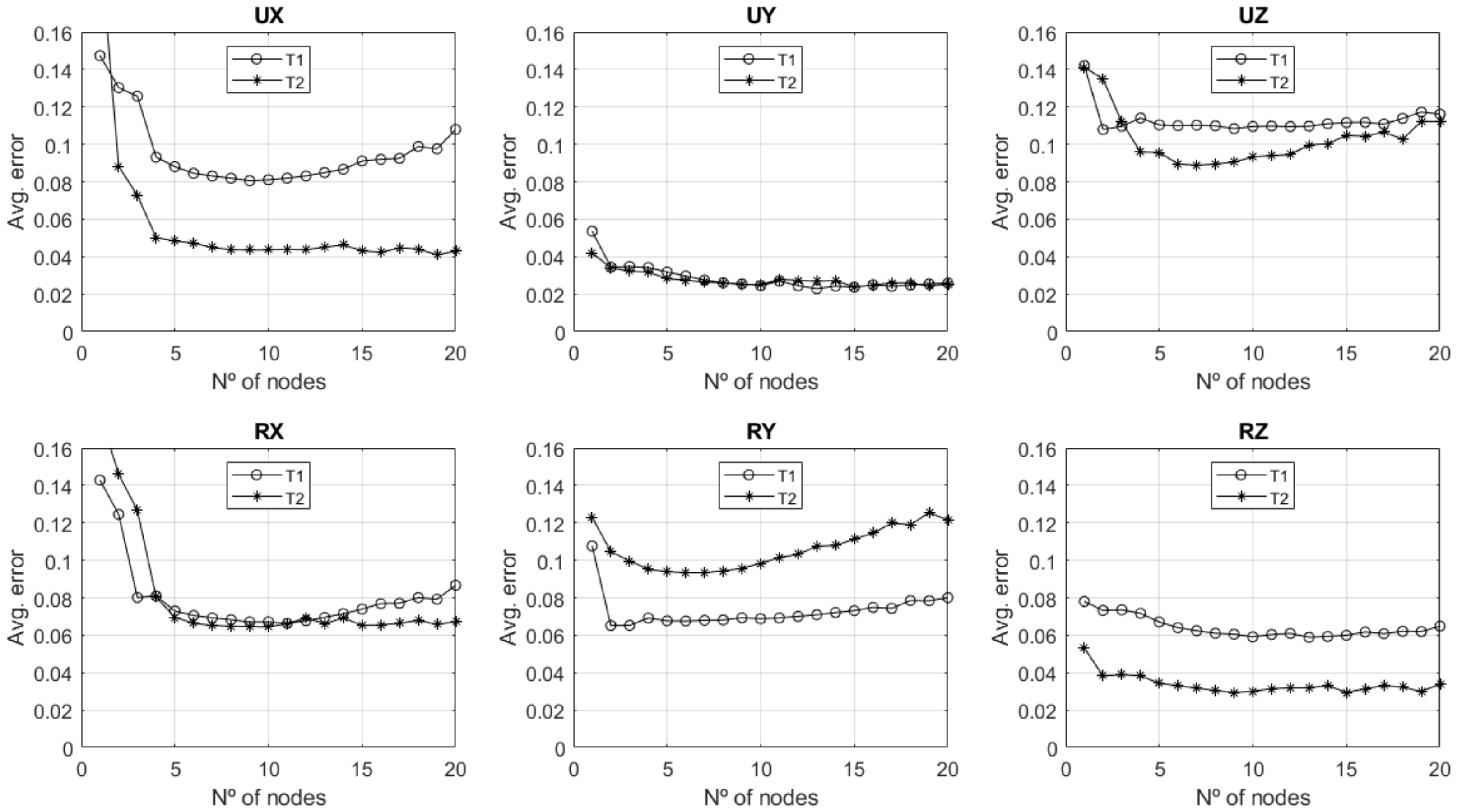
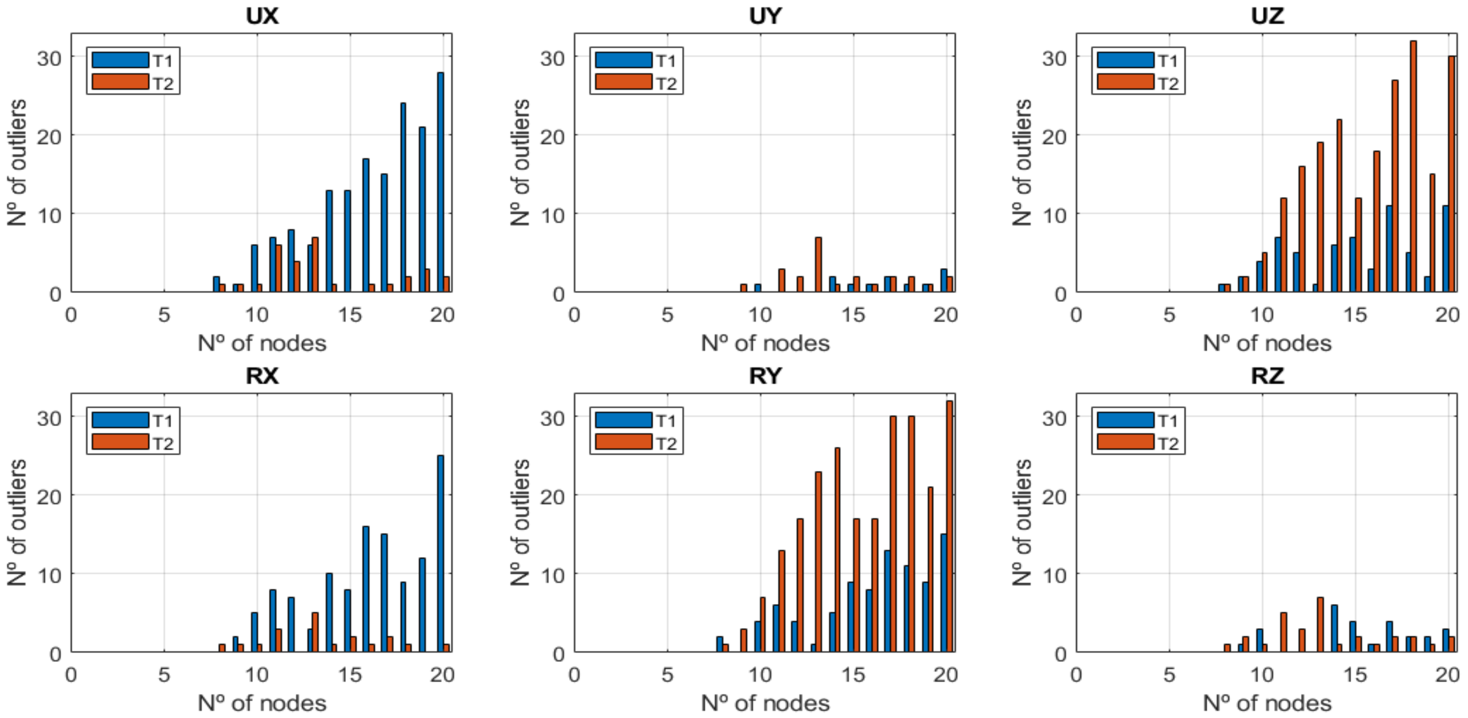
The obtained results show that there is a general increase in the accuracy of the networks when increasing the number of neurons up to 4 to 5. The optimal number of neurons was observed to be dependent on the joint configuration and the elastic element direction, ranging from 6 to 10, the use of more neurons increases the risk of obtaining isolated extremely bad predictions, probably due to over fitting.

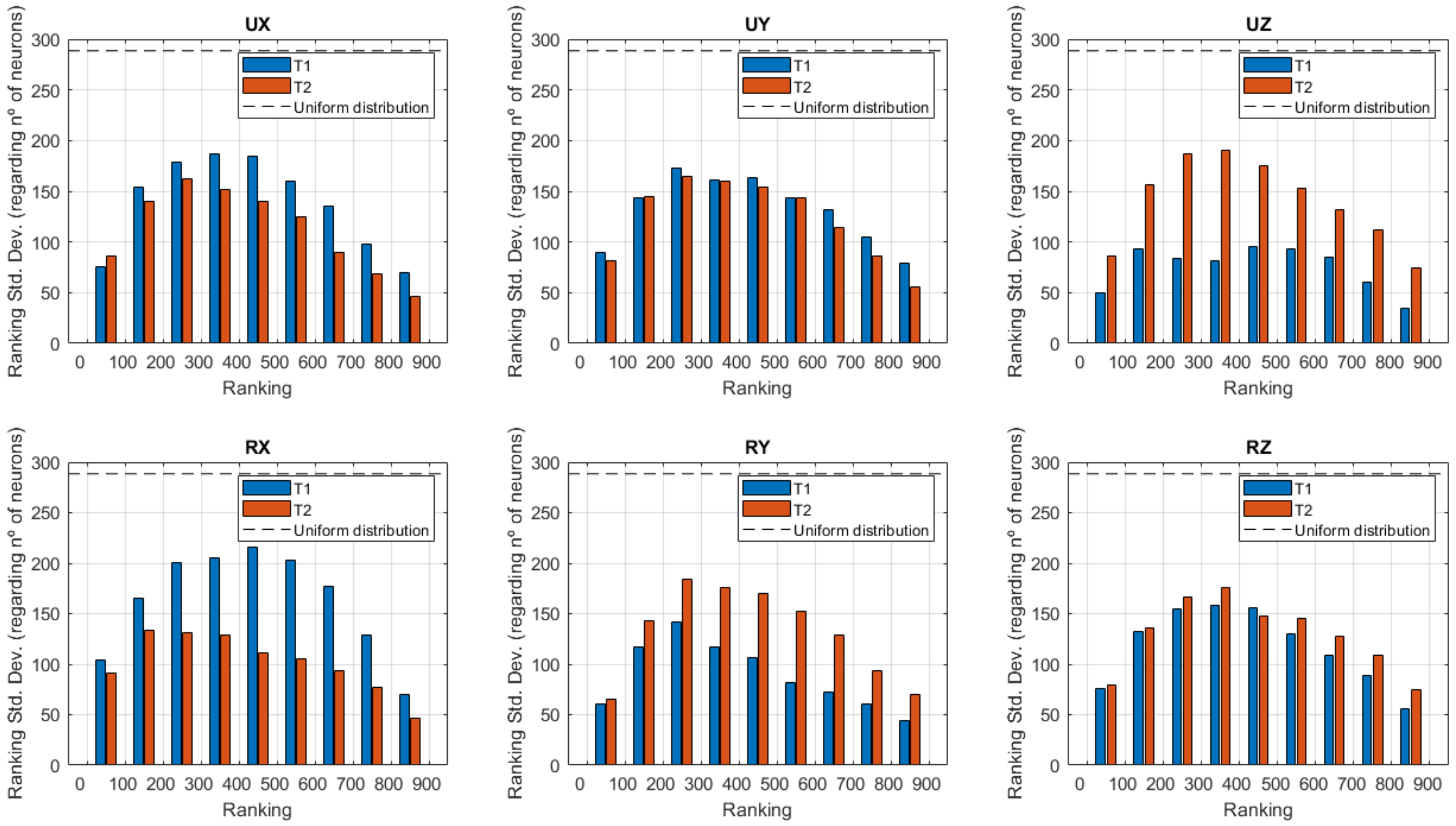
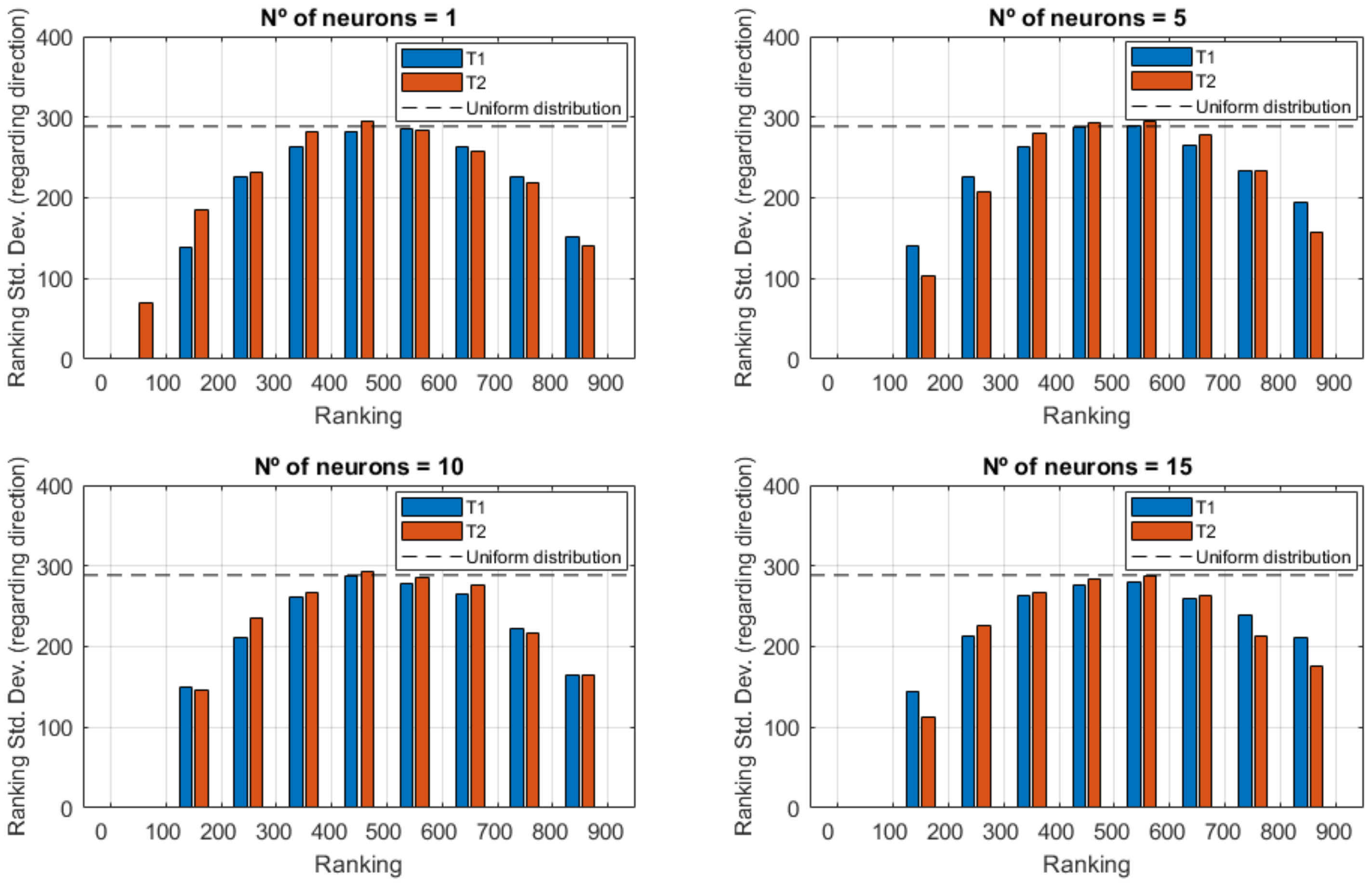
It was also found that there is a clear correlation between the accuracy of the network with respect to the number of neurons, meaning that if a certain training set presents high precision for a given number of neurons, it will also present the same tendency for the rest. With respect to the correlation of the accuracy of the networks with respect to the elastic element direction, it was only observed for extreme ranked networks, i.e., only if a given network is one of the best (or the worst) ranked for a specific direction, it will also tend to be one of the best (or the worst) for other directions. Both T1 and T2 joint configurations showed very similar behavior regarding these dependencies.

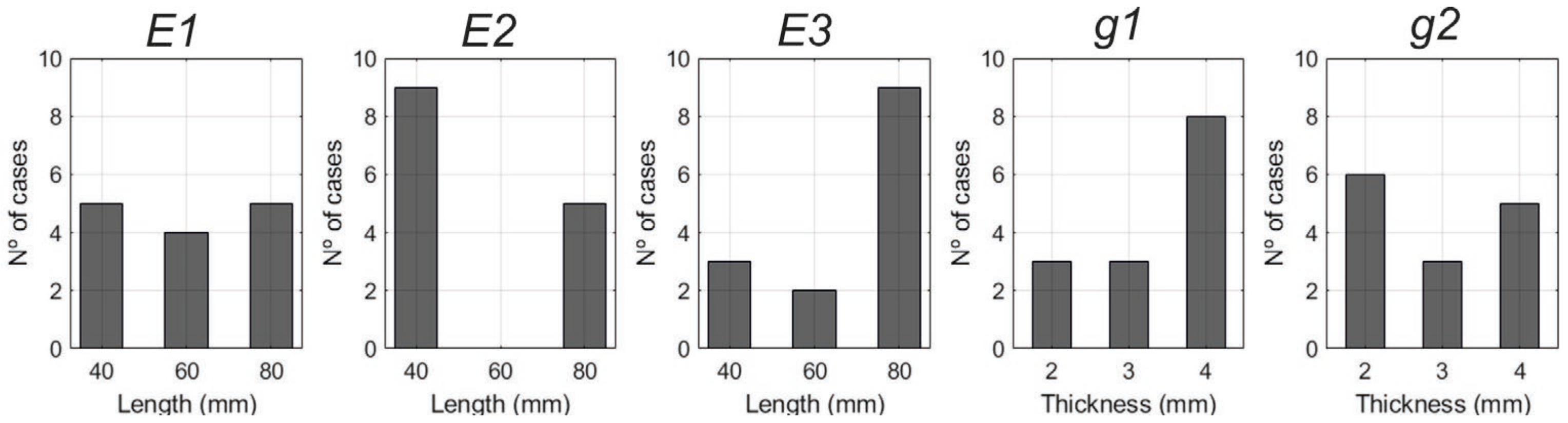
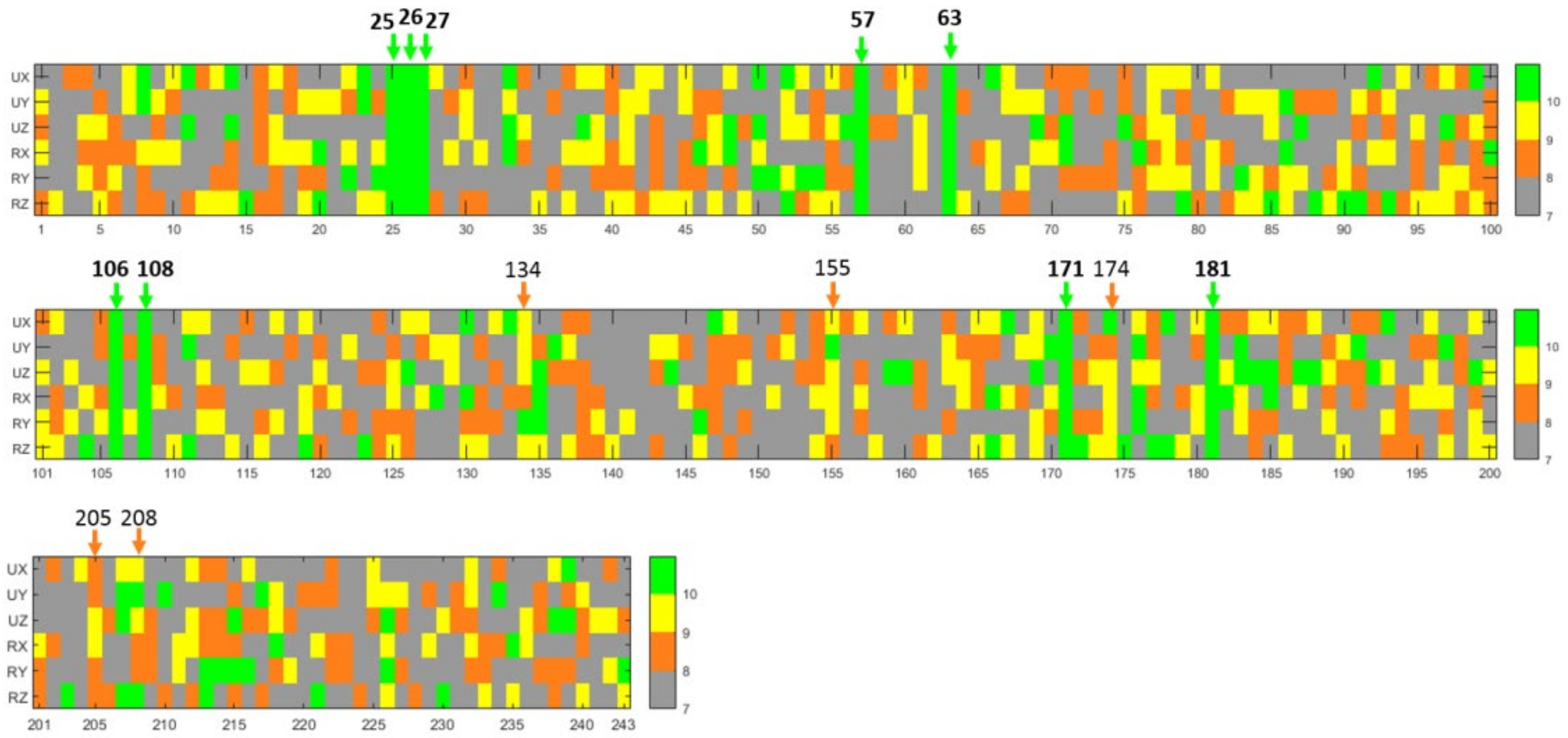
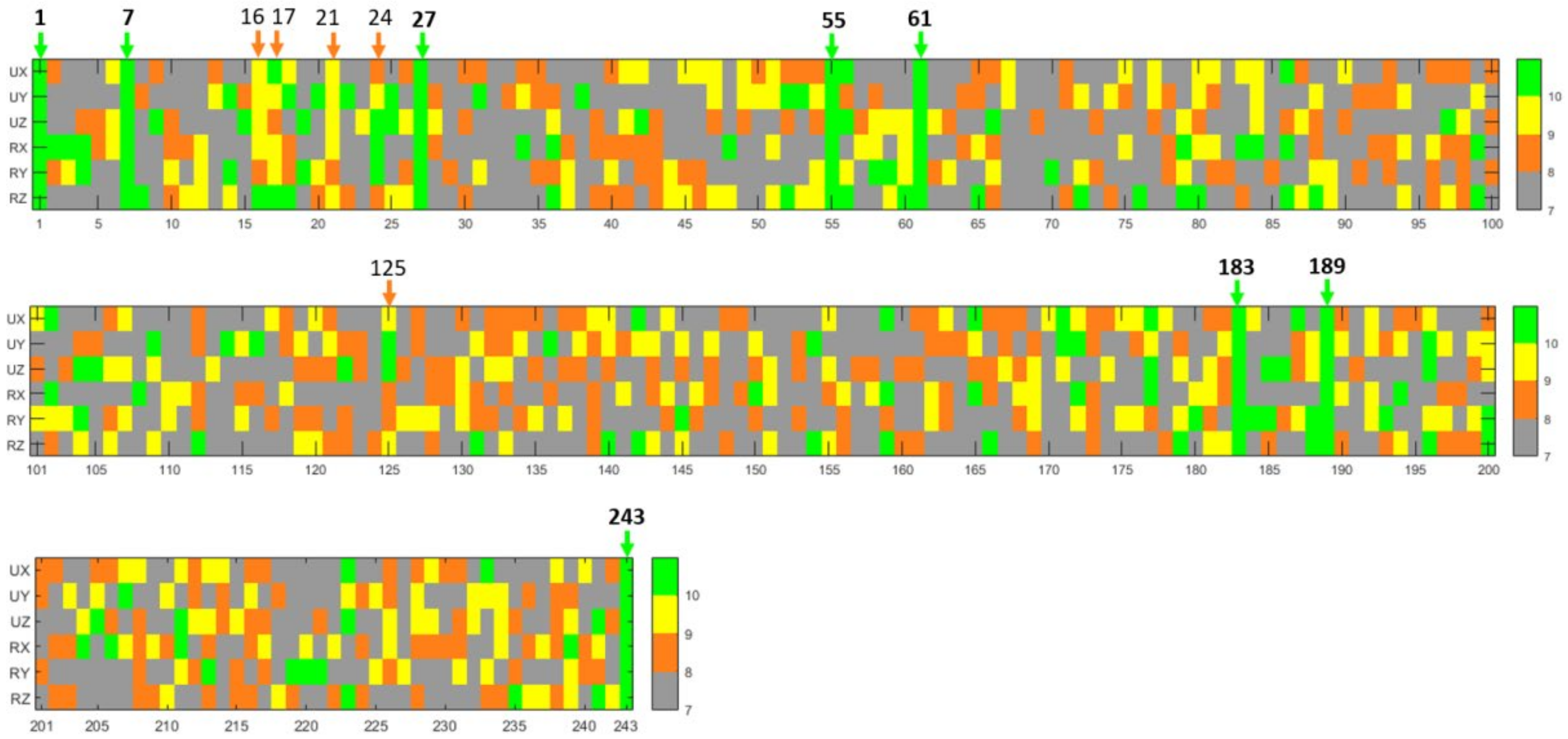
Additionally, there were located specific input data that appeared systematically in the 10 most accurate networks, regardless the spring direction. Although the same was observed for both joint configurations, the data that appeared systematically in T1 and in T2 were different. It was also found that these data had preference to contain certain variable values in the case of T1, lower values of E2 and higher values for E3 and g1 where observed, while T2 showed preference for lower values of E1 and E2, and higher values for g1.

A priori, no physical meaning was found to explain the behavior of the networks for this data. Consequently, it cannot be stated that similar behavior should be noticed in other structural problems. Future works would be needed to prove if these tendencies apply to data sets of similar problems or could be even extensive to data sets of completely different nature.

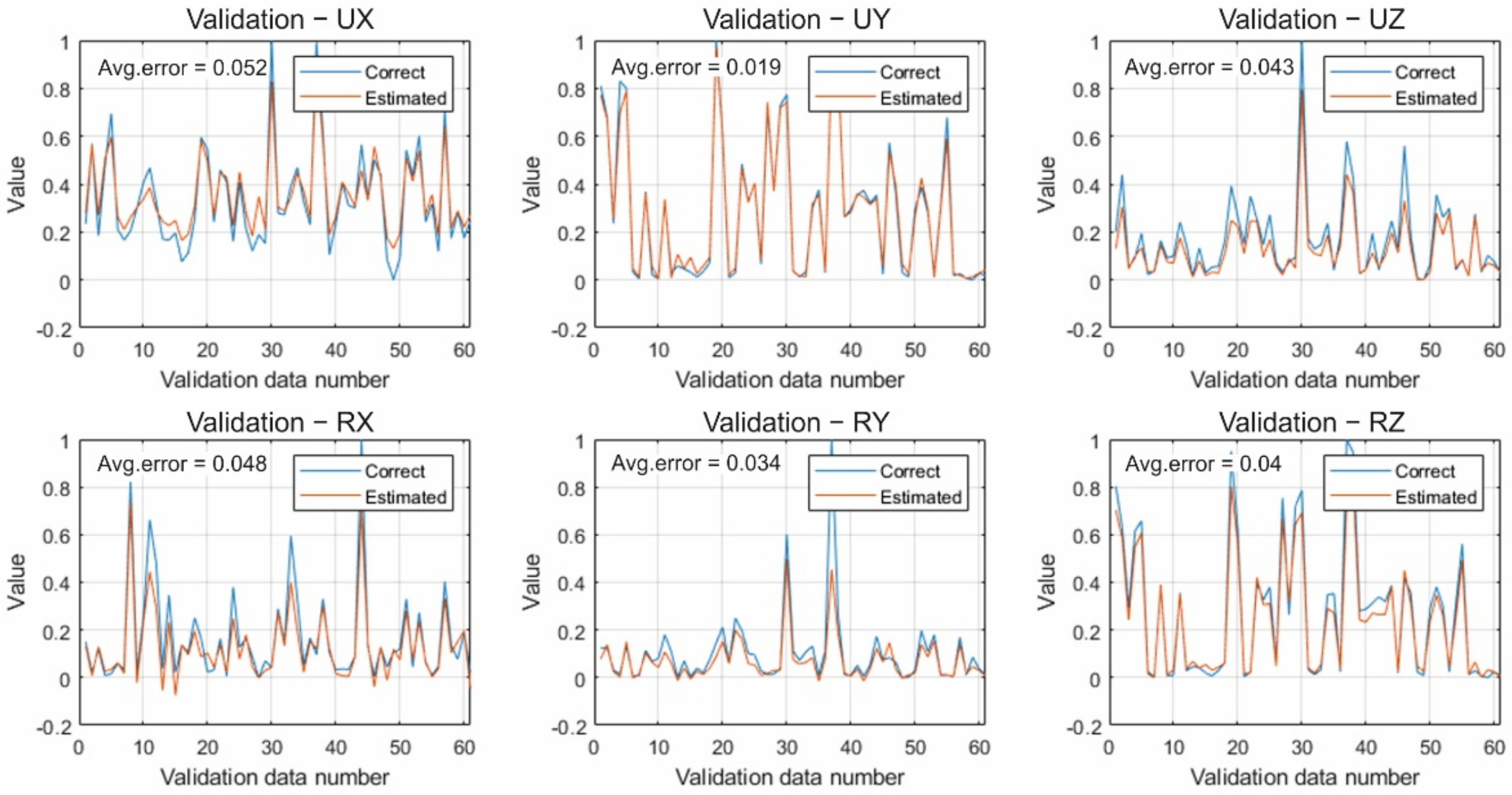
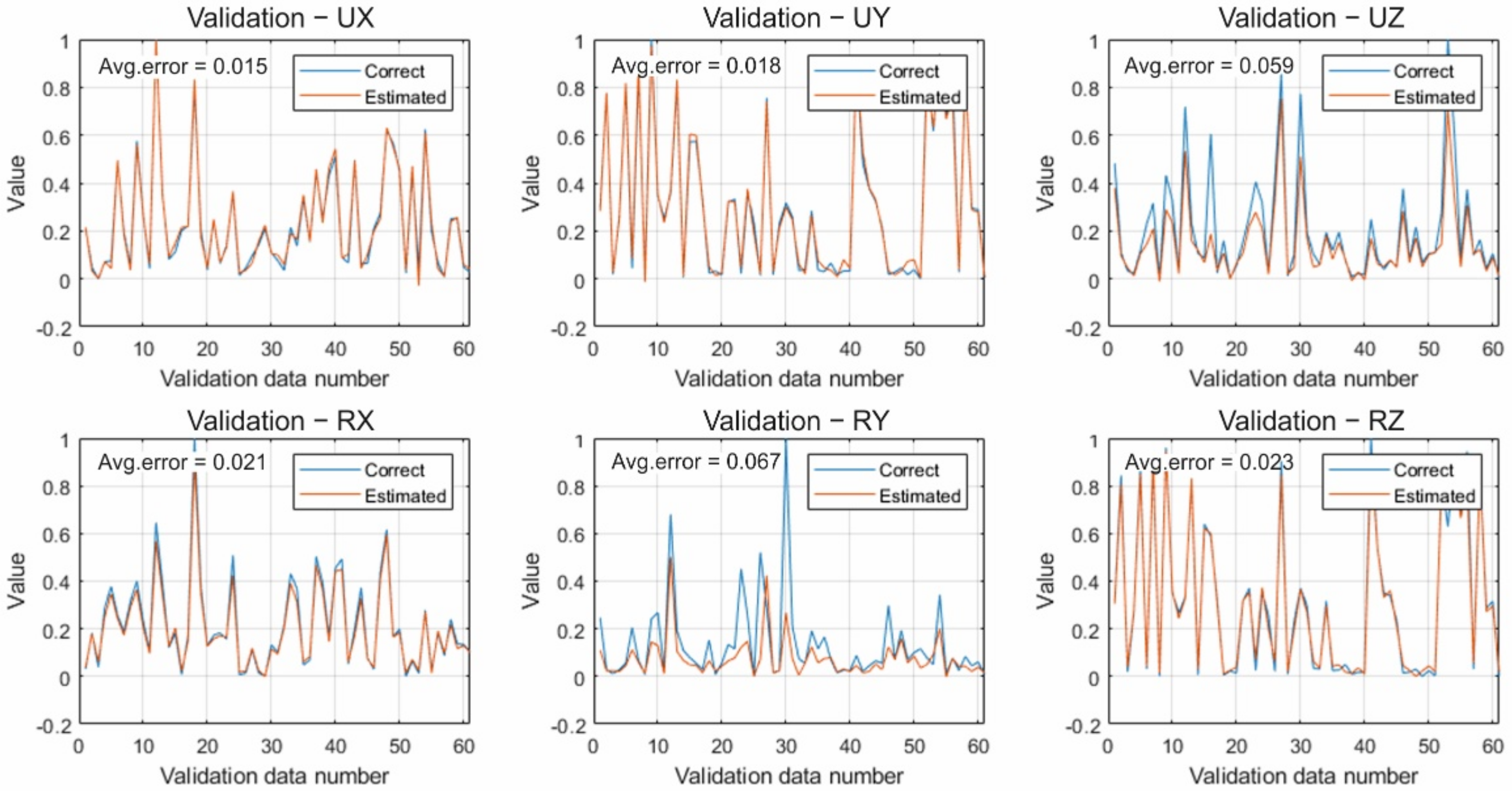
After running the 20,000 neural networks of the methodology, the least error networks for T1 and T2 were selected for validation. As it was proven, from about 10 neurons no accuracy improvement was observed at the same time the deviations on isolated predictions increased, so such selection was limited from 1 to 10 neurons. Validation results showed that some spring directions predictions were very close to the reference values, with average errors around 2%. The highest average error was of 6.7% corresponding to the Ry elastic element of the T2 junction.

From the performed study, it can be concluded that neural networks represent a solid alternative to the Bayesian Kriging regressions for the accuracy improvement of structural models constructed with beam type elements, as long as a proper selection of the training data set is assured through the presented methodology.

The present study provides a detailed insight on all the relevant aspects and difficulties that could be encountered when applying neural networks for the estimation of the elastic element stiffness in the alternative beam T-junction model studied. At the same time, it evaluates real aspects such as the generation of ANN with a reduced number of training data, the high sensitivity of the process to the selection of the initial sampling for training, and the deviation ranges that would be considered as acceptable so that any potential user could apply this methodology with a significant amount of confidence.

The interactions that take place at the joint level of T-junctions are complex and depend on the geometry of the junction, the type of loads and their direction. As it was pointed in the literature, these interactions are hard to characterize, and thus the alternative of presenting a complete methodology for the improvement of these T-junctions with a significant degree of confidence suppose a valuable tool for the structural design using finite element models.

5. Conclusions

In this paper the behavior of welded T-junctions in tubular structures was studied with the purpose of improving their behavior by means of artificial neural networks trained with finite element models. The topology of the junction at the joint level determines significant behavioral differences that cannot be taken into consideration with regular beam type elements.

To adjust their behavior to more precise results, elastic elements were introduced at the joint level, characterizing their stiffness utilizing artificial neural networks. In this paper the optimization and implementation of the validation data, through the creation of an optimal surrogate model based on neural networks was presented.

The results led to a model that predicted the stiffness of these elastic elements, in a satisfactory manner. The paper also focuses on how the neural network should be chosen, when training data is very limited and, more importantly, which of the available data should be used for training and which for validation.

The results indicated that the use of neural networks without a careful methodology in this type of problems could lead to inaccurate results.

The present work, more generally, is applicable to many other applications where there is insufficient training data (or data that costs a lot of time or money to obtain). This situation occurs in experimental trials, where the manufacture and use of the necessary test equipment to obtain more data is limiting. Furthermore, this situation appears in the computational calculation of complicated FEM or computational fluid dynamics (CFD) models, where a complicated calculation can take several hours and days and obtaining a large pool of data to train a neural network is pure utopia. In this sense, the methodology presented in this paper would be applicable to all these cases where data availability is scarce. The work presented is part of a broader development, where in the future it is expected to apply this methodology to larger problems based on this type of profiles, such as the study of bus structures.