Analytical Solution of the Three-Dimensional Laplace Equation in Terms of Linear Combinations of Hypergeometric Functions

Abstract

We present some solutions of the three-dimensional Laplace equation in terms of linear combinations of generalized hyperogeometric functions in prolate elliptic geometry, which simulates the current tokamak shapes. Such solutions are valid for particular parameter values. The derived solutions are compared with the solutions obtained in the standard toroidal geometry.

1. Introduction

In 2019, the European Union (27 countries) produced a total of around 617.52 Mtoe of electricity for its energy consumption needs, of which 100.63 Mtoe concern solid fossil fuels [1]. To produce energy of this magnitude, large quantities of fuel are required, at great expense. Fusion energy can provide a viable alternative energy source to fossil fuels.

One of the biggest obstacles to fusion is the question of how to hold the reactants long enough for the energy production to exceed the energy input. It is essential to understand the dynamics and confinement of plasma.

Recently, these types of experiments have been carried out with the help of Tokamak devices, which use a powerful magnetic field to confine the plasma to a toroidal shape. The tokamak is one of several types of magnetic confinement devices developed to produce controlled thermonuclear fusion energy. As of 2021, it is the leading candidate for a practical fusion reactor.

A crucial component in this task is the magnetohydrodynamic equilibrium (MHD) which defines the geometry of the confinement magnetic field. The MHD equations produce a second-order nonlinear differential equation known as the Grad–Shafranov equation [2,3], which is the equilibrium equation in MHD ideal for a two-dimensional plasma (e.g., axial-symmetric toroidal plasma in a tokamak). In axisymmetry the Grad–Shafranov equation is given by:

$$\frac{{\partial }^2\psi }{\partial R^2}-\frac{1}{R}\frac{\partial \psi }{\partial R}+\frac{{\partial }^2\psi }{\partial {\mathcal{Z}}^2}={\mu }_{0}R{J}_{\varphi },$$

where $J_{\varphi }$ is the toroidal plasma current, $\psi$ is the flux function and $(R,{\theta }^{*},\mathcal{Z}$) are the standard cylindrical coordinates.

The literature contains a large amount of scientific articles that address the tokamak balance problem, adopting different approaches.

For example, if the reference system is oblate toroidal, the Grad–Shafranov equation in vacuum admits an analytic solution highlighted in the works [4,5]. In case the source term assumes simple forms, the existence of analytical solutions of the nonlinear Grad–Shafranov equation has been shown [6,7,8,9].

The problem of finding the solution of the Grad–Shafranov equation was also addressed from the numerical point of view, through the development of some predictive equilibrium codes [10,11,12,13,14]. Semi-analytical methods have also been adopted in [15,16].

An interesting approach to analytically solve the Grad–Shafranov equation with non-constant source terms through the technique of separable variables was used in [17,18].

The exact analytical solution of the Grad–Shafranov equation in vacuum has been found only if the reference system has a standard circular shape or has an oblate elliptical toroidal geometry [4,5]. Both of these geometries are unsuitable for current tokamak experiments, which are all based on prolate elliptical geometry. In 2019, Crisanti cite Crisanti observed that, in axisymmetry, the Grad–Shafranov equation of vacuum coincides with the Laplace equation for the toroidal component of the vector potential. Cristanti faces the problem of finding the analytical solution for the Grad–Shafranov equation in vacuum (and therefore also of the Laplace equation) when the reference system is written in toroidal prolate elliptic cap-cyclide coordinates. A detailed study of the geometric and metric properties of these coordinates allows us to elaborate the analytical solution of both equations in terms of the Wangerin functions, the analytical expression of which is, however, not known.

The work of Crisanti [19] opens up the possibility of creating a reconstructive code of equilibrium based on an elongated geometry. Wangerin functions were first evaluated in [4]. However, to use them in a budget code, an independent evaluation and a cross-check will be required [19]. Furthermore, it will be necessary to evaluate the derivatives, to derive the poloidal magnetic field and find the Green’s function for this [19] geometry.

The literature shows us a wide range of scientific articles that address the problem of the analytical solution of the Laplace equation (in its various variants), see for example [20,21,22,23,24].

In this article, starting from the recent work of Crisanti [19], we transform the Laplace equation into the Heun equation, and based on the work of A.M. Ishkhanyan [25], we provide an analytical solution of the Laplace equation for some parameter values. Since the Laplace equation and the Grad–Shafranov equation differ by one sign, the procedure presented in this manuscript can be repeated to find the analytical solution of the Grad–Shafranov equation. In Section 2, we introduce the cap-cyclide geometry and, through some transformations of variables, we pass from the Grad–Shafranov equation to the Heun equation. In Section 3, we define the standard toroidal geometry as a special case of the cap-cyclide geometry. In Section 4 we find the analytical solution of the Laplace equation valid in standard toroidal geometry. In Section 5 we find the analytical solution of the Laplace equation in cap-cyclide coordinates for some parameter values. In Section 6, we present the conclusions.

1.1. Hypergeometric Functions

Definition 1. 

A hypergeometric series is formally defined as a power series

$$c_0+c_{1}z+c_2{z}^2+\dots =\sum _{n\ge 0}{c}_n{z}^n,$$

(1)

in which the ratio of successive coefficients is a rational function of n, that is

$$\frac{c_{n+1}}{c_n}=\frac{A\left(n\right)}{B\left(n\right)},$$

(2)

with $A\left(n\right)$ and $B\left(n\right)$ polynomials in n.

It is customary to assume $c_0$ to be 1. The polynomials $A\left(n\right)$ and $B\left(n\right)$ can be factored into linear factors of the form $(a_j+n)$ and $(b_k+n)$ respectively, where the $a_j$ and $b_k$ are complex numbers. For historical reasons, it is assumed that $(1+n)$ is a factor of $B\left(n\right)$.

The ratio between consecutive coefficients now has the form

$$\frac{c_{n+1}}{c_n}=\frac{c(a_1+n)\cdots (a_p+n)}{d(b_1+n)\cdots (b_q+n)(1+n)},$$

(3)

where c and d are the leading terms of $A\left(n\right)$ and $B\left(n\right)$. The series then has the form

$$1+\frac{a_1\cdots a_p}{b_1\cdots b_q·1}\frac{cz}{d}+\frac{a_1\cdots a_p}{b_1\cdots b_q·1}\frac{(a_1+1)\cdots (a_p+1)}{(b_1+1)\cdots (b_q+1)·2}{\left(\frac{cz}{d}\right)}^2+\cdots ,$$

(4)

or, by scaling z by the appropriate factor and rearranging

$$1+\frac{a_1\cdots a_p}{b_1\cdots b_q}\frac{z}{1!}+\frac{a_1(a_1+1)\cdots a_p(a_p+1)}{b_1(b_1+1)\cdots b_q(b_q+1)}\frac{z^2}{2!}+\cdots$$

(5)

This series is usually denoted by

$${}_p{F}_q(a_1,\dots ,a_p;b_1,\dots ,b_q;z).$$

(6)

The series, if convergent, defines a generalized hypergeometric function, which may then be defined over a wider domain of the argument by analytic continuation.

Historically, the most important are the functions of the form ${}_2{F}_1(a_1,a_2;b_1;z)$. These are sometimes called Gauss’s hypergeometric functions.

1.2. Heun Functions

Definition 2. 

The local Heun function $H(a,Q;\alpha ,\beta ,\gamma ,\delta ;z)$ (Karl L. W. Heun 1889) is the solution of Heun’s differential equation, that is

$$\frac{d^{2}H}{d{z}^2}+\left(\frac{\gamma }{z}+\frac{\delta }{z-1}+\frac{\epsilon }{z-a}\right)\frac{dH}{dz}+\frac{\alpha \beta z-Q}{z(z-1)(z-a)}H=0,$$

(7)

where $\epsilon$ is a real number such that the Fuchsian condition

$$\gamma +\delta +\epsilon =\alpha +\beta +1,$$

(8)

is satisfied. This relation is needed to ensure regularity of the point at ∞.

Function $H(a,Q;\alpha ,\beta ,\gamma ,\delta ;z)$ is holomorphic and such that $H(a,Q;\alpha ,\beta ,\gamma ,\delta ;0)=1$.

The local Heun function is called a Heun function if it is regular at $z=1$, and is called a Heun polynomial if it is regular at all three finite singular points $z=0,1,a$.

The complex number Q is called the accessory parameter. Heun’s equation has four regular singular points: $0,1,a$ and ∞ with exponents $(0,1-\gamma ),(0,1-\delta ),(0,1-\epsilon )$, and $(\alpha ,\beta )$.

2. From Grad–Shafranov Equation to Heun Equation

Starting from [19], the vacuum Grad–Shafranov equation are tackled in the elliptical prolate toroidal cap-cyclide coordinates framework.

In axisymmetric cylindrical coordinates $(R,{\vartheta }^{*},\mathcal{Z})$, ${\displaystyle \frac{\partial }{\partial {\vartheta }^{*}}=0}$, the vacuum Grad–Shafranov equation is given by:

$$\frac{{\partial }^2\psi }{\partial R^2}-\frac{1}{R}\frac{\partial \psi }{\partial R}+\frac{{\partial }^2\psi }{\partial {\mathcal{Z}}^2}=0.$$

(9)

This equation is formally similar to the Laplace equation:

$$\frac{{\partial }^2\psi }{\partial R^2}+\frac{1}{R}\frac{\partial \psi }{\partial R}+\frac{{\partial }^2\psi }{\partial {\mathcal{Z}}^2}=0.$$

(10)

(Note that Equations (9) and (10) differ for a sign in the first derivative part).

Consequently, it is obvious that any analytical solution found for the Laplace equation will be correlated to the analytical solution of the Grad–Shafranov equation.

For the present toroidal elongated tokamak, the most appropriate coordinate system is the cap-cyclide one [26], that is

$$\left\{\begin{array}{c}x=\frac{\mathsf{\Lambda }}{a_s\mathsf{\Gamma }}sn(\mu ,k)dn(\nu ,k_1)\cos \varphi ,\hfill \\ y=\frac{\mathsf{\Lambda }}{a_s\mathsf{\Gamma }}sn(\mu ,k)dn(\nu ,k_1)\sin \varphi ,\hfill \\ z=\frac{\sqrt{k}\mathsf{\Pi }}{2a_s\mathsf{\Gamma }},\hfill \end{array}\right.$$

(11)

where $(x,y,z)$ are the standard Cartesian coordinates, $dn,cn$, and $sn$ are the Jacobi elliptic functions, $a_s$ is a dimensional scale parameter and

$$\left\{\begin{array}{c}\mathsf{\Lambda }=1-d{n}^2(\mu ,k)s{n}^2(\nu ,k_1),\hfill \\ \mathsf{\Gamma }=s{n}^2(\mu ,k)d{n}^2(\nu ,k_1)+{\left[{\displaystyle \frac{\mathsf{\Lambda }}{\sqrt{k}}+cn(\mu ,k)dn(\mu ,k)sn(\nu ,k_1)cn(\nu ,k_1)}\right]}^2,\hfill \\ {\displaystyle \mathsf{\Pi }=\frac{{\mathsf{\Lambda }}^2}{k}-\left[s{n}^2(\mu ,k)d{n}^2(\nu ,k_1)+c{n}^2(\mu ,k)d{n}^2(\mu ,k)s{n}^2(\nu ,k_1)c{n}^2(\nu ,k_1)\right].}\hfill \end{array}\right.$$

(12)

The variation range of new variables $(\mu ,\nu ,\varphi )$ is defined as

$$0\le \mu \le \mathbf{K},0\le \nu \le {\mathbf{K}}^{\prime },0\le \varphi \le 2\pi .$$

Here $\mathbf{K}$ and $i\mathbf{K}$ are respectively the real and the imaginary complete elliptic integrals

$$\mathbf{K}\left(k\right)={\int }_0^{\frac{\pi }{2}}\frac{d\theta }{\sqrt{1-k^2{\sin }^2\theta }},\hspace{1em}i{\mathbf{K}}^{\prime }\left(k_1\right)=i{\int }_0^{\frac{\pi }{2}}\frac{d\theta }{\sqrt{1-k_1^2{\sin }^2\theta }},\hspace{1em}{k}^2+k_1^2=1,$$

where k and $k_1$ are respectively the parameter and the complementary parameter of the elliptic integrals.

By varying the parameter k, the coordinate transformation (11) describes a large set of quite different geometries [19]. For $\mu \mapsto 0$, independently of k, the geometry resembles the standard toroidal geometry; for larger values of $\mu$ the shape of the constant $\mu$ surfaces depend on the value of the k parameter. For $k\mapsto 0$ the surfaces tends to a bean shape. For intermediate values of k the surfaces can be either D or purely elliptical prolate shaped. For $k\mapsto 1$ all the surfaces are similar to the standard toroidal ones, independently of the value of $\mu$ [19].

As it is proved in [26] and subsequently reported by Crisanti [19], the Laplace Equation (10) in the cap-cyclide coordinates admits a quasi-separable solution of the type

$$\psi (\mu ,\nu ,\varphi )=\sqrt{\frac{\mathsf{\Gamma }}{\mathsf{\Lambda }}}M\left(\mu \right)N\left(\nu \right)\mathsf{\Phi }\left(\varphi \right),$$

(13)

where the functions $M\left(\mu \right),N\left(\nu \right),\mathsf{\Phi }\left(\varphi \right)$ satisfy the following ordinary differental equations

$$\left\{\begin{array}{c}{\displaystyle \frac{d^{2}M}{d{\mu }^2}+\frac{cn(\mu ,k)dn(\mu ,k)}{sn(\mu ,k)}\frac{dM}{d\mu }+\left[k^{2}s{n}^2(\mu ,k)-{\alpha }_2-{\alpha }_3\left(k^{2}s{n}^2(\mu ,k)+\frac{1}{s{n}^2(\mu ,k)}\right)\right]M=0,}\hfill \\ {\displaystyle \frac{d^{2}N}{d{\nu }^2}-k^2\frac{cn(\nu ,k)sn(\nu ,k)}{dn(\nu ,k)}\frac{dN}{d\nu }+\left[-d{n}^2(\nu ,k)+\frac{{\alpha }_2}{k^2}+{\alpha }_3\left(d{n}^2(\nu ,k)+\frac{k^2}{d{n}^2(\nu ,k)}\right)\right]N=0,}\hfill \\ {\displaystyle \frac{d^2\mathsf{\Phi }}{d{\varphi }^2}+{\alpha }_3\mathsf{\Phi }=0,}\hfill \end{array}\right.$$

(14)

with ${\alpha }_2=p^2$ and ${\alpha }_3=q^2$, p and q being constants, not necessarily integers [26].

In the rest of the paper, we refer to the Equation (14) as the Laplace equations.

The analytic solution of (14)${}_3$ is obtained immediately and is written as:

$$\mathsf{\Phi }\left(\varphi \right)=c_1\cos \left(\sqrt{{\alpha }_3}\varphi \right)+c_2\sin \left(\sqrt{{\alpha }_3}\varphi \right),c_1{c}_2\in \mathbb{R}.$$

(15)

From [19], by substituting $z_1=s{n}^2(\mu ,k)$ and $z_2=d{n}^2(\nu ,k)$, ($0\le z_1,z_2\le 1$) the two equations for $M\left(\mu \right)$ and $N\left(\nu \right)$ can be written as

$$\frac{d^{2}Z}{d{z}^2}+\frac{1}{2}\left(\frac{1}{z-1}+\frac{1}{z-a}+\frac{2}{z}\right)\frac{dZ}{dz}+\frac{1}{4}\frac{A_0+A_{1}z+A_2{z}^2}{(z-1)(z-a)z^2}Z=0,$$

(16)

where

$$\left\{\begin{array}{c}(z,a,A_0,A_1,A_2)=\left({\displaystyle z_1,\frac{1}{k^2},-\frac{q^2}{k^2},-\frac{p^2}{k^2},1-q^2}\right),\mathrm{for}\mathrm{equation}\mathrm{in}M\left(\mu \right)\hfill \\ (z,a,A_0,A_1,A_2)=\left({\displaystyle z_2,k^2,-q^2{k}^2,\frac{p^2}{k^2},1-q^2}\right),\mathrm{for}\mathrm{equation}\mathrm{in}N\left(\nu \right),\hfill \end{array}\right.$$

(17)

Following [25] and applying the transformation

$$Z=z^{\sigma }u\left(z\right),\hspace{1em}\sigma =\pm \sqrt{-\frac{A_0}{4a}}=\pm \frac{q}{2},$$

(18)

Equation (16) is reduced to the general Heun equation [25,27]

$$\frac{d^{2}u}{d{z}^2}+\left(\frac{\gamma }{z}+\frac{\delta }{z-1}+\frac{\epsilon }{z-a}\right)\frac{du}{dz}+\frac{\alpha \beta z-Q}{z(z-1)(z-a)}u=0,$$

(19)

where

$$\delta =\epsilon =\frac{1}{2},\gamma =1+2\sigma ,\alpha \beta =\sigma +\frac{a{A}_2-A_0}{4a},Q=\sigma \frac{a+1}{2}-\frac{A_0+a{A}_0+a{A}_1}{4a},$$

(20)

and under Fuchsian condition (8)

$$\alpha +\beta =\gamma .$$

(21)

Remark 1. 

Knowing the solution $u\left(z\right)$ of Heun’s Equation (19), it is consequential to go back to the solution of Wangerin’s Equation (16) given by

$$Z\left(z\right)=z^{\sigma }u\left(z\right),$$

so that, the solution of the Equation (14)${}_{1,2}$ in terms of μ and ν is given by

$$M\left(\mu \right)={\left({\mathrm{sn}}^2(\mu ,k)\right)}^{\sigma }u\left({\mathrm{sn}}^2(\mu ,k)\right),\hspace{1em}N\left(\nu \right)={\left({\mathrm{dn}}^2(\nu ,k_1)\right)}^{\sigma }u\left({\mathrm{dn}}^2(\nu ,k_1)\right)$$

3. Standard Toroidal Geometry as a Particular Case of Cap-Cyclide Geometry

As already pointed out in [19,26], if $k=1$ and $\mu \to 0$, the cap-cyclide geometry reduces to the standard toroidal one. Toroidal coordinates are a three-dimensional orthogonal coordinate system that results from rotating the two-dimensional bipolar coordinate system about the axis that separates its two foci. Thus, the two foci $F_1$ and $F_2$ in bipolar coordinates become a ring of radius a in the $xy$ plane of the toroidal coordinate system; the y-axis is the axis of rotation. The focal ring is also known as the reference circle. The toroidal coordinates are given by the following expressions [26]:

$$\begin{array}{ccc}\hfill x& =& a\frac{\sinh \mu }{\cosh \mu -\cos \nu }\cos \varphi ,\hfill \\ \hfill y& =& a\frac{\sinh \mu }{\cosh \mu -\cos \nu }\sin \varphi ,\hfill \\ \hfill z& =& a\frac{\sin \nu }{\cosh \mu -\cos \nu },\hfill \end{array}$$

(22)

together with $\mathrm{sign}\left(\mathrm{z}\right)=\mathrm{sign}\left(°\right)$ and $a\in \mathbb{R}$. The $\nu$ coordinate of a point P equals the angle $F_{1}P{F}_2$ and the $\mu$ coordinate equals the natural logarithm of the ratio of the distances $d_1$ and $d_2$ to opposite sides of the focal ring

$$\mu =\ln \frac{d_1}{d_2}.$$

The coordinate ranges are $-\pi <\nu \le \pi$, $\mu \ge 0$ and $0\le \varphi <2\pi$. Both geometries (standard toroidal and cap-cyclide) are obtained by rotating a two-dimensional coordinate system around the y axis, being respectively:

If $k=1$, then the two-dimensional coordinate system of cap-cyclide geometry becomes

$$\left\{\begin{array}{c}{\displaystyle x_{cc}{\mid }_{k=1}=\frac{\cosh \left(\mu \right)\sinh \left(\mu \right)}{a_s(\cosh \left(2\mu \right)+\sin \left(2\nu \right))},}\hfill \\ {\displaystyle z_{cc}{\mid }_{k=1}=\frac{\cos \left(2\nu \right)}{2a_s(\cosh \left(2\mu \right)+\sin \left(2\nu \right))}.}\hfill \end{array}\right.$$

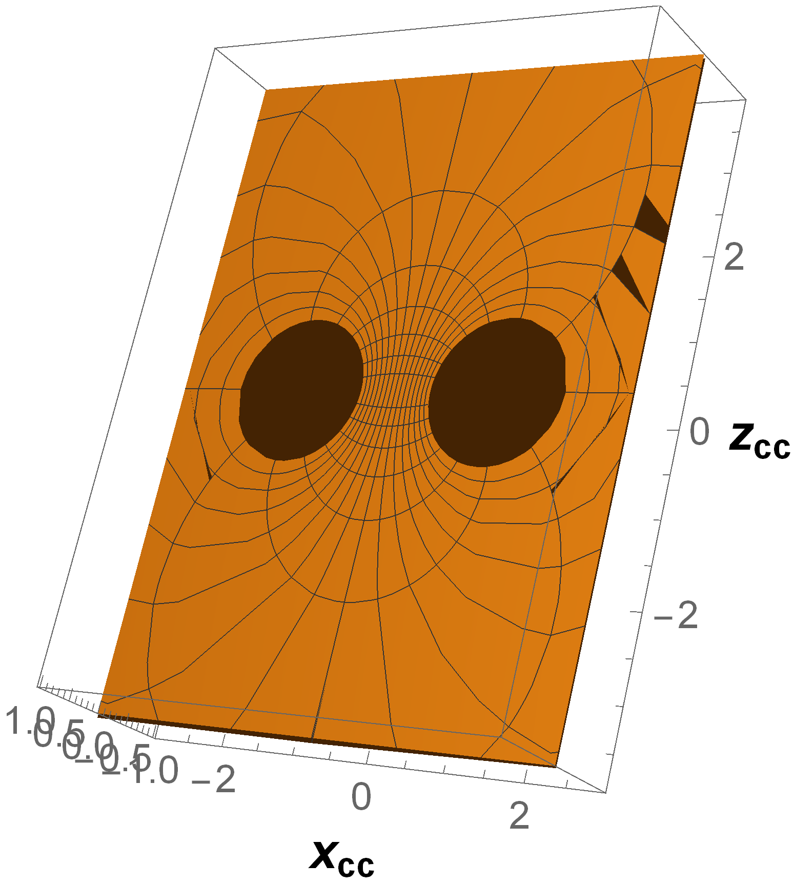
Moreover, when $\mu$ is close to zero, then the cap-cyclide bi-dimensional system approaches standard toroidal geometry, as in the Figure 1.

Figure 1. Two-dimensional coordinate system of cap-cyclide geometry with $k=1$ and $\mu$ close to 0.

We emphasize that even if in the limit for $\mu \to 0$ and $k=1$, the two geometries have the same shape, the metrics are different. In fact, the metric of the standard toroidal geometry is not obtained as a particular case of that of the cap-cyclide geometry (as also can be seen in [26]). This can also be noted in the formulas in Table 1: in fact even when $\mu \to 0$, $x_{st}\ne x_{cc}$ and $z_{st}\ne z_{cc}$.

Table 1. Two-dimensional coordinate system of standard toroidal and cap-cyclide geometries.

Standard Toroidal	Cap-Cyclide
$\left\{\begin{array}{c}{\displaystyle x_{st}=a\frac{\sinh \mu }{\cosh \mu -\cos \nu },}\hfill \\ {\displaystyle z_{st}=a\frac{\sin \nu }{\cosh \mu -\cos \nu },}\hfill \end{array}\right.$	$\left\{\begin{array}{c}{x}_{cc}=\frac{\mathsf{\Lambda }}{a_s\mathsf{\Gamma }}sn(\mu ,k)dn(\nu ,k_1)\hfill \\ z_{cc}=\frac{\sqrt{k}\mathsf{\Pi }}{2a_s\mathsf{\Gamma }}\hfill \end{array}\right.$

In [26], the authors obtained the analytic solution of Laplace equation in standard toroidal coordinates as

$$\psi (\mu ,\nu ,\varphi )=\sqrt{\cosh \mu -\cos \nu }H\left(\mu \right)\mathsf{\Theta }\left(\nu \right)\mathsf{\Phi }\left(\varphi \right),$$

(23)

where

$$\left\{\begin{array}{c}H\left(\mu \right)=A{\mathcal{P}}_{p-\frac{1}{2}}^q\left(\cosh \mu \right)+B{\mathcal{Q}}_{p-\frac{1}{2}}^q\left(\cosh \mu \right),\hfill \\ \mathsf{\Theta }\left(\nu \right)=A\sin \left(p\nu \right)+B\cos \left(p\nu \right),\hfill \\ \mathsf{\Phi }\left(\varphi \right)=A\sin \left(p\varphi \right)+B\cos \left(p\varphi \right)\hfill \end{array}\right.$$

(24)

where ${\mathcal{P}}_{p-\frac{1}{2}}^q,{\mathcal{Q}}_{p-\frac{1}{2}}^q$ are Legendre functions and A and B are constants.

4. Analytic Solution of Laplace Equation (14)${}_1$ in Standard Toroidal Geometry

In this section, we determine the analytic form of the solution of Equation (14)${}_1$ valid in standard toroidal geometry in terms of hypergeometric functions.

In the case of standard toroidal geometry, since $k=1$, then $a=1$ and Equation (16) becomes

$$\frac{d^{2}Z}{d{z}^2}+\left(\frac{1}{z-1}+\frac{1}{z}\right)\frac{dZ}{dz}+\frac{1}{4}\frac{A_0+A_{1}z+A_2{z}^2}{{(z-1)}^2{z}^2}Z=0,$$

(25)

with

$$\left\{\begin{array}{c}(z,a,A_0,A_1,A_2)=\left(z_1,1,-q^2,-p^2,1-q^2\right),\mathrm{for}\mathrm{equation}\mathrm{in}M\left(\mu \right),\hfill \\ (z,a,A_0,A_1,A_2)=\left(z_2,1,-q^2,p^2,1-q^2\right),\mathrm{for}\mathrm{equation}\mathrm{in}N\left(\nu \right).\hfill \end{array}\right.$$

(26)

After substitution (18), Equation (25) becomes

$$u^{″}\left(z\right)+\left(\frac{\gamma }{z}+\frac{\delta +\epsilon }{z-1}\right)u^{\prime }\left(z\right)+\frac{\alpha \beta z-Q}{z{(z-1)}^2}u\left(z\right)=0,$$

(27)

where

$$\delta =\epsilon =\frac{1}{2},\gamma =1+2\sigma ,\alpha \beta =\sigma +\frac{1}{4},Q=\sigma +\frac{2q^2-A_1}{4}.$$

(28)

The last equation is the Heun Equation (19) for $k=1$. Let

$$c=\frac{1}{2}\left(\gamma -\alpha -\beta -\sqrt{{(\gamma -\alpha -\beta )}^2-4\alpha \beta +4Q}\right).$$

Since, in our case, Fuchsian condition reduces to $\alpha +\beta =\gamma$, then

$$c=-\sqrt{Q-\alpha \beta }.$$

Following [28], consider the change of the dependent variable $u\left(z\right)={(z-1)}^{c}G\left(z\right)$. After substitution, from Equation (27), we get a hypergeometric equation

$$z(z-1)G^{″}\left(z\right)+\left[(2c+\alpha +\beta +1)z-\gamma \right]G^{\prime }\left(z\right)+(c+\alpha )(c+\beta )G\left(z\right)=0,$$

(29)

whose general solution is given by

$$\begin{array}{ccc}\hfill G\left(z\right)& =& c_1{}_2{F}_1\left(c+\alpha ,c+\beta ;\gamma ;z\right)+\hfill \\ & +& c_2{(-1)}^{1-\gamma }{z}^{1-\gamma }{}_2{F}_1\left(1+c+\alpha -\gamma ,1+c+\beta -\gamma ;2-\gamma ;z\right),\hfill \end{array}$$

(30)

with $c_1,c_2\in \mathbb{C}$. Thus, the analytic solution of the Heun Equation (27) is given as

$$\begin{array}{ccc}\hfill u\left(z\right)& =& {(z-1)}^c[c_1{}_2{F}_1\left(c+\alpha ,c+\beta ;\gamma ;z\right)+\hfill \\ & +& c_2{(-1)}^{1-\gamma }{z}^{1-\gamma }{}_2{F}_1\left(1+c+\alpha -\gamma ,1+c+\beta -\gamma ;2-\gamma ;z\right)],\hfill \end{array}$$

(31)

with $c_1,c_2\in \mathbb{C}$. Accordingly, the analytic solution of Equation (14)${}_1$ for $k=1$ reads

$$\begin{array}{ccc}M\left(\mu \right)& =& {\left({\mathrm{sn}}^2\left(\mu \right)\right)}^{\sigma }{\left({\mathrm{sn}}^2\left(\mu \right)-1\right)}^c[c_1{}_2{F}_1\left(c+\alpha ,c+\beta ;\gamma ;{\mathrm{sn}}^2\left(\mu \right)\right)\hfill \\ & +& c_2{(-1)}^{1-\gamma }{\left({\mathrm{sn}}^2\left(\mu \right)\right)}^{1-\gamma }{}_2{F}_1\left(1+c+\alpha -\gamma ,1+c+\beta -\gamma ;2-\gamma ;{\mathrm{sn}}^2\left(\mu \right)\right)],\hfill \end{array}$$

(32)

with $c_1,c_2\in \mathbb{C}$. Similarly, the analytic solution of Equation (14)${}_2$ for $k=1$ reads

$$\begin{array}{ccc}N\left(\nu \right)& =& {\left({\mathrm{dn}}^2\left(\nu \right)\right)}^{\sigma }{\left({\mathrm{dn}}^2\left(\nu \right)-1\right)}^c[c_1{}_2{F}_1\left(c+\alpha ,c+\beta ;\gamma ;{\mathrm{dn}}^2\left(\nu \right)\right)\hfill \\ & +& c_2{(-1)}^{1-\gamma }{\left({\mathrm{dn}}^2\left(\nu \right)\right)}^{1-\gamma }{}_2{F}_1\left(1+c+\alpha -\gamma ,1+c+\beta -\gamma ;2-\gamma ;{\mathrm{dn}}^2\left(\nu \right)\right)].\hfill \end{array}$$

(33)

5. Analytic Solutions of Laplace Equation (14)${}_1$ in Cap-Cyclide Geometry

In this section, we determine the analytical form of the solution of Equation (14)${}_1$ valid in the cap-cyclide geometry in terms of hypergeometric functions and for particular values of the parameters.

Let’s solve the Heun Equation (19) first.

Following [25], we impose that the following series developed around the singularity $z=a$:

$$u={\left(\frac{z-a}{1-a}\right)}^{\mu }\sum _{n=0}^{+\infty }{c}_n{\left(\frac{z-a}{1-a}\right)}^n,\mu =0,1-\epsilon$$

(34)

is a solution of the Heun equation and that it reduces to a generalized hypergeometric function.

Let q be integer. This condition will allow us to construct a solution in terms of hypergeometric functions.

Let $\mu =0$. The generalized hypergeometric function ${}_r{F}_s$ is defined as the series [29]

$${}_r{F}_s\left(a_1,\dots ,a_r;b_1,\dots ,b_s;\frac{z-a}{1-a}\right)=\sum _{n=0}^{\infty }{c}_n{\left(\frac{z-a}{1-a}\right)}^n,$$

where the coefficients satisfy the two-term recurrence relation

$$\frac{c_n}{c_{n-1}}=\frac{1}{n}\frac{{\displaystyle \prod _{k=1}^r(a_k-1+n)}}{{\displaystyle \prod _{k=1}^s(b_k-1+n)}}.$$

Since q is integer, then $\gamma$ is also integer. Assume that $\gamma$ is negative, i.e., $\gamma =-N,N=1,2,3,\dots$. Following [25], we set $r=N+2$, $s=N+1$, and

$$a_1,\dots ,a_N,a_{N+1},a_{N+2}=1+e_1,\dots ,1+e_N,\alpha ,\beta ,$$

$$b_1,\dots ,b_N,b_{N+1}=e_1,\dots ,e_N,\epsilon ,$$

with $e_1,\dots ,e_N$ being certain constants.

It can be shown that the Heun Equation (19) admits the following solution [25]

$$u={}_{N+2}{F}_{1+N}\left(1+e_1,\dots ,1+e_N,\alpha ,\beta ;e_1,\dots ,e_N,\epsilon ;\frac{z-a}{1-a}\right).$$

(35)

if and only if the following polynomial $\mathsf{\Pi }\left(n\right)$ in an auxiliary variable n is identically zero [25]:

$$\begin{array}{ccc}\mathsf{\Pi }\left(n\right)& =& R_n\frac{(\alpha -1+n)(\beta -1+n)}{n(\epsilon -1+n)}\prod _{k=1}^N(e_k+n)+{\mathcal{Q}}_{n-1}\prod _{k=1}^N(e_k-1+n)+\hfill \\ & +& P_{n-2}\frac{(n-1)(\epsilon -2+n)}{(\alpha -2+n)(\beta -2+n)}\prod _{k=1}^N(e_k-2+n),\hfill \end{array}$$

(36)

where

$$\begin{array}{ccc}{R}_n& =& -an(\epsilon -1+n),\hfill \\ {\mathcal{Q}}_n& =& n\left[(a-1)(n+\alpha +\beta )+a(n-1)\right]+n(\delta +a\epsilon )+a\alpha \beta -Q,\hfill \\ P_n& =& (1-a)(\alpha +n)(\beta +n).\hfill \end{array}$$

(37)

The term of degree $N+2$ in $\mathsf{\Pi }\left(n\right)$ is automatically canceled, while the term of degree $N+1$ is zero owing to the Fuchsian condition. Then, by canceling the coefficients of the polynomial $\mathsf{\Pi }\left(n\right)$, we obtain a system of $N+1$ algebraic equations, N of which are used to determine the N constants $e_1,\dots ,e_N$ and the last equetion imposes a restriction on the accessory parameter Q: this restriction is obtained by substituting the expressions of the constants $e_1,\dots ,e_N$ in the last equation thus arriving at a polynomial equation of degree $N+1$ in the variable Q.

Therefore, there are many solutions of Equation (19) in terms of a single generalized hypergeometric function ${}_r{F}_s$ if $\gamma$ is a negative interger and the accessory parameter Q satisfies a certain polynomial equation [25].

Similarly, another solution can be constructed in terms of a power series in the vicinity of the singularity $z=1$:

$$u={\left(\frac{z-1}{a-1}\right)}^{\mu }\sum _{n=0}^{+\infty }{c}_n{\left(\frac{z-1}{a-1}\right)}^n,\mu =0,1-\delta .$$

(38)

Let $\mu =0$. Such a series can be reduced to a generalized hypergeometric series for any negative integer $\gamma =-N,N=1,2,3,\dots$ [25], i.e.,

$$u={}_{N+2}{F}_{1+N}\left(1+s_1,\dots ,1+s_N,\alpha ,\beta ;s_1,\dots ,s_N,\delta ;\frac{z-1}{a-1}\right).$$

(39)

The accessory parameter Q and the parameters $s_1,s_2,\dots ,s_N$ involved in solution (39) are determined from a system of $N+1$ algebraic equations constructed by equating the coefficients of the following polynomial $\tilde{\mathsf{\Pi }}\left(n\right)$ in an auxiliary variable n to zero [25]:

$$\begin{array}{ccc}\tilde{\mathsf{\Pi }}\left(n\right)& =& {\tilde{R}}_n\frac{(\alpha -1+n)(\beta -1+n)}{n(\delta -1+n)}\prod _{k=1}^N(e_k+n)+{\tilde{\mathcal{Q}}}_{n-1}\prod _{k=1}^N(e_k-1+n)+\hfill \\ & +& {\tilde{P}}_{n-2}\frac{(n-1)(\delta -2+n)}{(\alpha -2+n)(\beta -2+n)}\prod _{k=1}^N(e_k-2+n),\hfill \end{array}$$

(40)

where

$$\begin{array}{ccc}\hfill {\tilde{R}}_n& =& -n(\delta -1+n),\hfill \\ \hfill {\tilde{\mathcal{Q}}}_n& =& n\left[(1-a)(n+\alpha +\beta )+n-1\right]+n(\delta +a\epsilon )+\alpha \beta -Q,\hfill \\ \hfill {\tilde{P}}_n& =& (a-1)(\alpha +n)(\beta +n).\hfill \end{array}$$

(41)

The restrictions imposed on Q obtained from the polynomial $\mathsf{\Pi }\left(n\right)$ (36) and then from the polynomial $\tilde{\mathsf{\Pi }}\left(n\right)$ (40) are identical.

The two solutions (35) and (39) are linearly independent, indeed their Wronskian turns out to be:

$$\begin{array}{ccc}W\left(z\right)& =& \frac{\alpha \beta }{(a-1)e_1{e}_2\dots e_N{s}_1{s}_2\dots s_N\delta \epsilon }[(1+e_1)(1+e_2)\dots (1+e_N)s_1{s}_2\dots s_N\delta ·\hfill \\ & ·& {}_{N+2}{F}_{N+1}\left(2+e_1,2+e_2,\dots ,2+e_N,1+\alpha ,1+\beta ;1+e_1,1+e_2,\dots ,1+e_N,1+\epsilon ;\frac{z-a}{1-a}\right)·\hfill \\ & ·& {}_{N+2}{F}_{N+1}\left(1+s_1,1+s_2,\dots ,1+s_N,\alpha ,\beta ;s_1,s_2,\dots ,s_N,\delta ;\frac{z-1}{a-1}\right)+\hfill \\ & +& e_1{e}_2\dots e_N(1+s_1)(1+s_2)\dots (1+s_N)\epsilon ·\hfill \\ & ·& {}_{N+2}{F}_{N+1}\left(1+e_1,1+e_2,\dots ,1+e_N,\alpha ,\beta ;e_1,e_2,\dots ,e_N,\epsilon ;\frac{z-a}{1-a}\right)·\hfill \\ & ·& {}_{N+2}{F}_{N+1}\left(2+s_1,2+s_2,\dots ,2+s_N,1+\alpha ,1+\beta ;1+s_1,1+s_2,\dots ,1+s_N,1+\delta ;\frac{z-1}{a-1}\right)]\ne 0\hfill \end{array}$$

Thus, if $\gamma =-N$, $N\in \mathbb{Z}$ and Q satisfies a certain polynomial equation of $N+1$ degree, the general solution of the Heun Equation (19) is given by:

$$\begin{array}{ccc}u\left(z\right)& =& c_1{}_{N+2}{F}_{N+1}\left(1+e_1,\dots ,1+e_N,\alpha ,\beta ;e_1,\dots ,e_N,\epsilon ;\frac{z-a}{1-a}\right)+\hfill \\ & +& c_2{}_{N+2}{F}_{N+1}\left(1+s_1,\dots ,1+s_N,\alpha ,\beta ;s_1,\dots ,s_N,\delta ;\frac{z-1}{a-1}\right),c_1,c_2\in \mathbb{C}.\hfill \end{array}$$

(42)

Similarly, the general analytic solution of Laplace equation is given by:

$$\begin{array}{ccc}M\left(\mu \right)& =& {\mathrm{sn}}^{2\sigma }(\mu ,k)[c_1{}_{N+2}{F}_{N+1}\left(1+e_1,\dots ,1+e_N,\alpha ,\beta ;e_1,\dots ,e_N,\epsilon ;\frac{{\mathrm{sn}}^2(\mu ,k)-a}{1-a}\right)+\hfill \\ & +& c_2{}_{N+2}{F}_{N+1}\left(1+s_1,\dots ,1+s_N,\alpha ,\beta ;s_1,\dots ,s_N,\delta ;\frac{{\mathrm{sn}}^2(\mu ,k)-1}{a-1}\right)],c_1,c_2\in \mathbb{C}.\hfill \end{array}$$

(43)

Now we write hypergeometric solution of the Heun equation for some values of parameter $\gamma$.

5.1. Case: $N=0\Rightarrow \gamma =0$

In this case, the Heun equation becomes

$$\frac{d^{2}u}{d{z}^2}+\left(\frac{\delta }{z-1}+\frac{\epsilon }{z-a}\right)\frac{du}{dz}+\frac{\alpha \beta z-Q}{z(z-1)(z-a)}u=0,$$

(44)

and admits a solution in terms of the ordinary hypergeometric function:

$$u=c_1{}_2{F}_1\left(\alpha ,\beta ;\epsilon ;\frac{z-a}{1-a}\right)+c_2{}_2{F}_1\left(\alpha ,\beta ;\delta ;\frac{z-1}{a-1}\right),c_1,c_2\in \mathbb{C}.$$

(45)

Since the Fuchsian condition (8) reduces to $\alpha +\beta =0$, from Equations (36) and (40), we obtain the restriction on Q

$$Q=0.$$

(46)

• ${\displaystyle \sigma =\frac{q}{2}}$
  From $\gamma =0$, we get $q=-1$ and Fuchsian condition (8) $\alpha =-\beta$. Furthermore, from Equation (17)${}_1$ we obtain

  $$a=\frac{1}{k^2},A_0=-\frac{1}{k^2},A_1=-\frac{p^2}{k^2},A_2=0,\mathrm{for}\mathrm{equation}\mathrm{in}M\left(\mu \right).$$

  (47)
  Since ${\displaystyle \alpha \beta =\sigma +\frac{a{A}_2-A_0}{4a}}$, then from Equation (47), we get

  $${\alpha }_{1,2}=\pm \frac{1}{2},{\beta }_{1,2}=\mp \frac{1}{2}.$$
  The expression ${\displaystyle Q=\sigma \frac{a+1}{2}-\frac{A_0+a{A}_0+a{A}_1}{4a}}$, together with Equation (46), gives

  $$\frac{p^2}{4k^2}=0.$$
  Thus we get $p^2=0$. Consequently, Heun equation reduces to

  $$u^{″}\left(z\right)+\left(\frac{1}{2(z-1)}+\frac{1}{2(z-a)}\right)u^{\prime }\left(z\right)-\frac{z}{4z(z-1)(z-a)}=0,$$

  (48)

  whose solution, $\forall k$ is given by

  $$\begin{array}{c}u=c_1{}_2{F}_1\left(\frac{1}{2},-\frac{1}{2};\frac{1}{2};\frac{z-a}{1-a}\right)+c_2{}_2{F}_1\left(\frac{1}{2},-\frac{1}{2};\frac{1}{2};\frac{z-1}{a-1}\right)\forall z\in [0,1].\end{array}$$

  (49)
  Hence, the solution of the corresponding Wangerin Equation (16) $\forall k$ is given by

  $$\begin{array}{ccc}Z\left(z\right)& =& \frac{1}{\sqrt{z}}[c_1{}_2{F}_1\left(\frac{1}{2},-\frac{1}{2};\frac{1}{2};\frac{z-a}{1-a}\right)+\hfill \\ \hspace{1em}& +& c_2{}_2{F}_1\left(\frac{1}{2},-\frac{1}{2};\frac{1}{2};\frac{z-1}{a-1}\right)]\forall z\in (0,1].\hfill \end{array}$$

  (50)
  The solution of the corresponding (14)${}_1$ equation $\forall 0<k<1$ is given by

  $$\begin{array}{ccc}\hfill M\left(\mu \right)& =& \frac{1}{\sqrt{{\mathrm{sn}}^2(\mu ,k)}}[c_1{}_2{F}_1\left(\frac{1}{2},-\frac{1}{2};\frac{1}{2};\frac{{\mathrm{sn}}^2(\mu ,k)-a}{1-a}\right)+\hfill \\ & +& c_2{}_2{F}_1\left(\frac{1}{2},-\frac{1}{2};\frac{1}{2};\frac{{\mathrm{sn}}^2(\mu ,k)-1}{a-1}\right)],\hfill \end{array}$$

  (51)
  $\forall \mu \in (0,\mathbf{K}]$.
• ${\displaystyle \sigma =-\frac{q}{2}\Rightarrow }$ The same solution as for $q=1$!

5.2. Case $N=1,\hspace{1em}\Rightarrow \hspace{1em}\gamma =-1$

In this case, the Heun equation becomes

$$\frac{d^{2}u}{d{z}^2}+\left(-\frac{1}{z}+\frac{\delta }{z-1}+\frac{\epsilon }{z-a}\right)\frac{du}{dz}+\frac{\alpha \beta z-Q}{z(z-1)(z-a)}u=0,$$

(52)

and admits a solution in terms of the generalized hypergeometric function:

$$u=c_1{}_3{F}_2\left(1+e_1,\alpha ,\beta ;e_1,\epsilon ;\frac{z-a}{1-a}\right)+c_2{}_3{F}_2\left(1+s_1,\alpha ,\beta ;s_1,\delta ;\frac{z-1}{a-1}\right),c_1,c_2\in \mathbb{C},$$

(53)

with constants $e_1,s_1$. Since the Fuchsian condition (8) reduces to $\alpha +\beta =-1$, the polynomials (36) and (40) give

$$e_1=-\frac{a\alpha \beta }{Q},s_1=-\frac{\alpha \beta }{Q}.$$

(54)

Besides, the accessory parameter Q satisfies the following polinomial equation of second degree

$$2Q^2-\left(1+a\right)Q+2a\alpha \beta =0.$$

(55)

• ${\displaystyle \sigma =\frac{q}{2}}$
  From $\gamma =-1$, we get $q=-2$ and the Fuchsian condition (8) reads $\alpha =-\beta -1$. Besides, from Equation (17) we obtain

  $$a=\frac{1}{k^2},A_0=-\frac{4}{k^2},A_1=-\frac{p^2}{k^2},A_2=-3,\mathrm{for}\mathrm{equation}\mathrm{in}M\left(\mu \right)$$

  (56)
  Since ${\displaystyle \alpha \beta =\sigma +\frac{a{A}_2-A_0}{4a}}$, then from Equation (56), we get

  $${\alpha }_1=-\frac{3}{2},{\beta }_1=\frac{1}{2},\hspace{1em}{\alpha }_2=\frac{1}{2},{\beta }_2=-\frac{3}{2}$$
  From Equation (55), we get the Q values

  $$Q_{1,2}=\frac{1}{4}\left(1+\frac{1}{k^2}\pm \sqrt{1+\frac{14}{k^2}+\frac{1}{k^4}}\right).$$

  (57)
  The expression ${\displaystyle Q=\sigma \frac{a+1}{2}-\frac{A_0+a{A}_0+a{A}_1}{4a}}$ gives the relation between k and p

  $$\frac{1+\left(1\pm \sqrt{1+\frac{1}{k^4}+\frac{14}{k^2}}\right)k^2+p^2}{4k^2}=0.$$

  (58)
  The Heun equation reduces to

  $$u^{″}\left(z\right)+\left(-\frac{1}{z}+\frac{1}{2(z-1)}+\frac{1}{2(z-a)}\right)u^{\prime }\left(z\right)-\frac{\frac{3}{4}z+Q}{z(z-1)(z-a)}=0$$

  (59)

  whose solution, $\forall k$ is given by

  $$u=c_1{}_3{F}_2\left(1+e_1,-\frac{3}{2},\frac{1}{2};e_1,\frac{1}{2};\frac{z-a}{1-a}\right)+c_2{}_3{F}_2\left(1+s_1,-\frac{3}{2},\frac{1}{2};s_1\frac{1}{2};\frac{z-1}{a-1}\right),$$

  (60)
  $c_1,c_2\in \mathbb{C}$ and $z\in [0,1]$.
  Hence, the solution of the corresponding Wangerin equation for any k is given by

  $$\begin{array}{ccc}Z\left(z\right)& =& \frac{1}{z}[c_1{}_3{F}_2\left(1+e_1,-\frac{3}{2},\frac{1}{2};e_1,\frac{1}{2};\frac{z-a}{1-a}\right)+\hfill \\ \hspace{1em}& +& c_2{}_3{F}_2\left(1+s_1,-\frac{3}{2},\frac{1}{2};s_1\frac{1}{2};\frac{z-1}{a-1}\right)],\hfill \end{array}$$

  (61)
  $c_1,c_2\in \mathbb{C}$ and $z\in (0,1]$.
  Consequently, the solution of the corresponding (14)${}_1$ is written as

  $$\begin{array}{ccc}M\left(\mu \right)& =& \frac{1}{{\mathrm{sn}}^2(\mu ,k)}[c_1{}_3{F}_2\left(-\frac{3}{2},\frac{1}{2},1+e_1;\frac{1}{2},e_1;\frac{{\mathrm{sn}}^2(\mu ,k)-a}{1-a}\right)+\hfill \\ \hspace{1em}& +& c_2{}_3{F}_2\left(-\frac{3}{2},\frac{1}{2},1+s_1;\frac{1}{2},s_1;\frac{{\mathrm{sn}}^2(\mu ,k)-1}{a-1}\right)],\hfill \end{array}$$

  (62)
  $c_1,c_2\in \mathbb{C}$ and $\mu \in (0,\mathbf{K}]$.
• ${\displaystyle \sigma =-\frac{q}{2}\Rightarrow }$ The same solution as for $q=2$.

5.3. Positive Integer $\gamma$

Let $\gamma$ now be a positive integer. Following [25], we apply a change of the dependent variable in order to obtain a Heun equation with altered parameters and with a negative characteristic exponent $\gamma$. Let $u=z^{1-\gamma }w$: this change transforms the Heun equation into another Heun equation with the altered parameter ${\gamma }^{*}=2-\gamma$, i.e.,

$$w^{″}\left(z\right)+\left(\frac{{\gamma }^{*}}{z}+\frac{\delta }{z-1}+\frac{\epsilon }{z-a}\right)w^{\prime }\left(z\right)+\frac{{\alpha }^{*}{\beta }^{*}z-Q^{*}}{z(z-1)(z-a)}w\left(z\right)=0,$$

(63)

where ${\alpha }^{*}=(\alpha +1-\gamma ),{\beta }^{*}=(\beta +1-\gamma )$ and $Q^{*}=Q+(1-\gamma )(\epsilon +a\delta )$.

Then, for $\gamma \ge 2$, we have a Heun equation with a zero or negative integer ${\gamma }^{*}=-N,$$N=1,2,3,\dots .$. As a result, we obtain the solution

$$\begin{array}{ccc}u& =& z^{1-\gamma }[c_1{}_{N+2}{F}_{1+N}\left(e_1+1,\dots ,e_N+1,\alpha +1-\gamma ,\beta +1-\gamma ;e_1,\dots ,e_N,\epsilon ;\frac{z-a}{1-a}\right)+\hfill \\ & +& c_2{}_{N+2}{F}_{1+N}\left(s_1+1,\dots ,s_N+1,\alpha +1-\gamma ,\beta +1-\gamma ;s_1,\dots ,s_N,\delta ;\frac{z-1}{a-1}\right)].\hfill \end{array}$$

(64)

The only exception is the case $\gamma =1$: we do not know an ${}_r{F}_s$ solution in this exceptional case [25].

$\gamma =2$

In this case, the Heun equation becomes

$$\frac{d^{2}u}{d{z}^2}+\left(\frac{2}{z}+\frac{\delta }{z-1}+\frac{\epsilon }{z-a}\right)\frac{du}{dz}+\frac{\alpha \beta z-Q}{z(z-1)(z-a)}u=0.$$

(65)

• Let ${\displaystyle \sigma =\frac{q}{2}}$
  From $\gamma =2$, we have $q=1$ and from Fuchsian condition (8) we have $\alpha =2-\beta$. Besides, from Equation (17) we obtain

  $$a=\frac{1}{k^2},A_0=-\frac{1}{k^2},A_1=-\frac{p^2}{k^2},A_2=0,\mathrm{for}\mathrm{equation}\mathrm{in}M\left(\mu \right)$$

  (66)
  Since ${\displaystyle \alpha \beta =\sigma +\frac{a{A}_2-A_0}{4a}}$, then from Equation (66), we get

  $${\alpha }_1=\frac{1}{2},{\alpha }_2=\frac{3}{2},\hspace{1em}{\beta }_1=\frac{3}{2},{\beta }_2=\frac{1}{2},$$

  and expression ${\displaystyle Q=\sigma \frac{a+1}{2}-\frac{A_0+a{A}_0+a{A}_1}{4a}}$ gives

  $$Q=\frac{2+2k^2+p^2}{4k^2}.$$
  Consider the change ${\displaystyle u=\frac{w}{z}}$. We obtain another Heun equation that reads as:

  $$\frac{d^{2}w}{d{z}^2}+\left(\frac{{\gamma }^{*}}{z}+\frac{\delta }{z-1}+\frac{\epsilon }{z-a}\right)\frac{dw}{dz}+\frac{{\alpha }^{*}{\beta }^{*}z-Q^{*}}{z(z-1)(z-a)}w=0,$$

  (67)

  with ${\gamma }^{*}=0$, ${\alpha }^{*}=\alpha -1,{\beta }^{*}=\beta -1$ and $Q^{*}=Q-(a\delta +\epsilon )$.
  We already know the solution of Equation (67) which for any k is written as

  $$w\left(z\right)=c_1{}_2{F}_1\left({\alpha }^{*},{\beta }^{*};\epsilon ;\frac{z-a}{1-a}\right)+c_2{}_2{F}_1\left({\alpha }^{*},{\beta }^{*};\delta ;\frac{z-1}{a-1}\right),{\alpha }^{*}=\frac{1}{2},{\beta }^{*}=-\frac{1}{2},$$

  with $c_1,c_2\in \mathbb{C}$, ${\left(p^{*}\right)}^2=0$ and $Q^{*}=0$. Consequently, $Q=a\delta +\epsilon$ and we get the relation between k and p

  $$\frac{p^2}{4k^2}=0.$$

  (68)
  Thus, the solution of the Heun Equation (65) for any k is given by

  $$u\left(z\right)=\frac{1}{z}\left[c_1{}_2{F}_1\left({\alpha }^{*},{\beta }^{*};\epsilon ;\frac{z-a}{1-a}\right)+c_2{}_2{F}_1\left({\alpha }^{*},{\beta }^{*};\delta ;\frac{z-1}{a-1}\right)\right],$$

  (69)

  with ${\displaystyle {\alpha }^{*}=\frac{1}{2},{\beta }^{*}=-\frac{1}{2},c_1,c_2\in \mathbb{C}}$ and $z\in (0,1]$.
  Hence, the solution of the corresponding Wangerin equation for any k is given by

  $$Z\left(z\right)=\frac{1}{\sqrt{z}}\left[c_1{}_2{F}_1\left({\alpha }^{*},{\beta }^{*};\epsilon ;\frac{z-a}{1-a}\right)+c_2{}_2{F}_1\left({\alpha }^{*},{\beta }^{*};\delta ;\frac{z-1}{a-1}\right)\right],$$

  (70)

  with ${\displaystyle {\alpha }^{*}=\frac{1}{2},{\beta }^{*}=-\frac{1}{2},c_1,c_2\in \mathbb{C}}$ and $z\in (0,1]$.
  The solution of the corresponding Equation (14)${}_1$ for any $0<k<1$ is given by

  $$\begin{array}{ccc}M\left(\mu \right)& =& \frac{1}{\sqrt{{\mathrm{sn}}^2(\mu ,k)}}[c_1{}_2{F}_1\left({\alpha }^{*},{\beta }^{*};\epsilon ;\frac{{\mathrm{sn}}^2(\mu ,k)-a}{1-a}\right)+\hfill \\ \hspace{1em}& +& c_2{}_2{F}_1\left({\alpha }^{*},{\beta }^{*};\delta ;\frac{{\mathrm{sn}}^2(\mu ,k)-1}{a-1}\right)],\hfill \end{array}$$

  (71)

  with ${\displaystyle {\alpha }^{*}=\frac{1}{2},{\beta }^{*}=-\frac{1}{2},c_1,c_2\in \mathbb{C}}$ and $\mu \in (0,\mathbf{K}]$
• ${\displaystyle \sigma =-\frac{q}{2}\Rightarrow }$ The same solution as for $q=-1$.

6. Conclusions and Discussion

In this paper, we have presented the analytic solution of Laplace’s Equation (14)${}_1$ in terms of linear combinations of generalized hypergeometric functions which hold for integer values of $\gamma$ and when the accessory parameter Q satisfies a particular polynomial equation, the degree of which is related to the value of the integer $\gamma$. $\gamma$ being an integer is not a particularly significant limitation, since $\gamma =2\sigma +1=q+1$ and q is generally an integer.

The second Laplace Equation (14)${}_2$ still remains to be solved: it too is reduced to a Heun equation (but with different parameters) and can therefore be solved with the technique applied here.

Once this is done, the complete solution of the three-dimensional Laplace Equation is constructed.

At this respect, since the Laplace equation and the Grad–Shafranov equation differ by one sign (plus instead of minus in the term of the first derivative), one can also apply the technique presented in this manuscript to the Grad–Shafranov equation to construct its solution in terms of a linear combination of hypergeometric functions. We will investigate these latter aspects in future work.