1. Introduction
One of the main continuous models is a dynamic system described by an autonomous system of ordinary differential equations, that is, a system of equations of the form:
where
t is an independent variable commonly interpreted as time,
are the coordinates of a moving point or several points. In practice, the right-hand sides
are often rational or algebraic functions of coordinates
or can be reduced to such a form by a certain change of variables.
The problem of the numerical integration of the dynamical system (1) consists of finding its solution at the moment of time
up to an error value that does not exceed the given boundary
. One of the simplest ways to solve this problem is based on using explicit difference schemes, e.g., Runge–Kutta schemes [
1].
A priori estimates of the accuracy exponentially depend on the value of
T and therefore, in practice, one tries to avoid such estimates when performing calculations for sufficiently long times. Usually, one tries to estimate the error, either by comparing the solutions obtained with different steps, according to the Richardson method [
2,
3], or by observing the change in quantities that should remain constant for the exact solution. If the dynamical system under consideration has a considerable amount of conservation laws, then one usually monitors the changes in the algebraic integrals of motion ([
4], § 164).
The idea to construct difference schemes that precisely preserve the integrals of motion in dynamical systems arose in the late 1980s. In the works of Cooper [
5] and Yu. B. Suris [
6,
7], a large family of Runge–Kutta schemes was discovered that preserve all the polynomial first- and second-order integrals of motion as well as on the symplectic structure in Hamiltonian systems [
8,
9]. For a number of dynamical systems, this family of schemes preserves all algebraic integrals. For example, if we exclude the Kovalevskaya case from consideration, any integral of the rigid body problem with a fixed point is expressed in terms of the known number of quadratic integrals [
10], therefore, symplectic schemes preserve all algebraic integrals of this system.
However, as has been shown both analytically and in a series of numerical experiments, symplectic schemes do not exactly preserve higher-order integrals [
8]. Nevertheless, the first finite-difference scheme for the many-body problem [
11], preserving all classical integrals of motion, was proposed in 1992 by Greenspan [
12]. He only published his results in 1995 [
13,
14], and more recently in the monograph [
15]. Independently and in a somewhat different form, this scheme was proposed in 1995 by Simo and González [
16], as it was mentioned by Graham et al. [
17]. Greespan’s scheme is a kind of combination of the midpoint method and discrete gradient method [
18,
19] preserving a number of symmetries of the initial problem [
12].
In the 2000s, several general approaches for the construction of difference schemes were proposed that preserve all algebraic integrals of motion. To our opinion, these methods can be divided into two large groups: the methods based on the modification of the Runge–Kutta schemes, and the methods used certain transformations of the original differential system. The first group includes the parametric symplectic partitioned Runge–Kutta method [
20,
21], in which the Runge–Kutta method is considered with the order of approximation chosen such that there is a free parameter in the procedure of determining the Butcher matrix coefficients. This parameter can be chosen to preserve a chosen quadratic integral.
The invariant energy quadratization method (IEQ, recently proposed by Yang et al. [
22,
23]) can be considered to be a member of the second group. Based on this method, for a number of Hamiltonian systems including the two-body problem (Kepler problem), Hong Zhang et al. [
24] constructed finite-difference schemes conserving the energy. The IEQ method suggests finding such a change of variables, after which the energy becomes a quadratic form, so that the standard simplectic Runge–Kutta schemes, written for this transformed system, conserve its energy. The procedure admits the increasing number of unknowns and the loss of the non-Hamiltonian form of equations.
Both the symplectic Runge–Kutta schemes and the Greenspan scheme are implicit. Therefore, during numerical integration according to these schemes, a system of algebraic equations is numerically solved at each step. As a result, the integrals are not exactly preserved, but with a noticeably higher accuracy in comparison with explicit schemes.
To preserve the changes in the integrals at the round-off error level, one can use difference schemes that do not exactly preserve the integrals but preserve them up to the terms whose order in the step
is much higher than the order of the scheme itself. These schemes include the large family of schemes implementing the Hamiltonian boundary value methods [
25]. Within this approach, the energy of a Hamiltonian system is not exactly conserved, but in any given order of approximation in
([
25], th. 3.4). Moreover, as shown in a number of numerical experiments with periodic solutions ([
25], § 4.4), the total energy variation fluctuates within the round-off error without a noticeable trend towards dissipation or anti-dissipation. This circumstance favorably distinguishes this class of schemes from explicit Runge–Kutta schemes, in which the energy usually monotonically increases or decreases.
On the other hand, it should be noted that the advantages of symplectic schemes and various geometric integrators preserving algebraic integrals over other schemes in numerical integration for long times are not at all so obvious and were the subject of a number of discussions [
26]. The point is that in the case of non-integrable systems, while remaining on the integral manifold, we can decline far from the exact solution. Nevertheless, in the course of searching for numerical methods for integrating dynamical systems, a very interesting construction was found—a difference scheme of a dynamical system that preserves all algebraic integrals of motion ([
8], § IV). In our opinion, this scheme is a difference mathematical model of the same phenomenon, the continuous model of which is the dynamical system.
Attempts have been made for a long time to consider Newton’s equations as difference equations ([
27], ch. 2, § 3), but with the standard discretization, such a representation faces a violation of the fundamental conservation laws. Implicit difference schemes provide approximations that satisfy these laws. Moreover, for linear models, the approximate solution found by conservative schemes also inherits other properties of the exact solution, including periodicity [
28]. The purpose of our research was to develop methods for construction and investigation by purely algebraic methods of this kind of discrete models of dynamical systems.
One of the important steps in this direction is the development of methods for constructing various conservative difference schemes for the most famous family of dynamical systems, the many-body problem. Since we have at our disposal a large and well-studied family of schemes that preserve linear and quadratic integrals, i.e., the symplectic Runge–Kutta schemes, the simplest way to construct such schemes is to introduce additional variables with respect to which all algebraic integrals of the many-body problem are expressed in terms of linear and quadratic integrals. This assumption can be considered as a development of the invariant energy quadratization method. Bearing in mind the further study of schemes in computer algebra systems, we, in contrast to Greenspan, immediately tried to get rid of the radicals in the right-hand sides of the equations.
The introduction of additional variables in the construction of difference schemes is known as the scalar auxiliary variable approach (SAV), proposed by Jie Shen et al. [
29]. In the past, every effort was made to perform replacements that preserve the symplectic structure of the many-body problem. In particular, when studying the simple collision of two bodies, the aim was to find not just a regularizing transformation, but a canonical transformation. Due to this, the famous Weierstrass theorem on simple collisions was considered to be an obstacle [
30]. There is, however, a simple way to find a regularizing transformation, which was proposed by Burdet [
31] and Heggie [
32] and is thoroughly described in the book by Marchal ([
11], ch. 6).
One of the delicate features of the IEQ method is the preservation of constraints. The fact is that when additional variables are introduced, the equations describe the relation between the coordinates and velocities of bodies, on the one hand and the auxiliary variables on the other hand. In the IEQ method, these equations are not necessarily quadratic, so these constraints are not exactly preserved. We argue that it is possible if one looks at such a change of variables that describes all integrals of motion and all constraint equations be by quadratic functions. Therefore, in this paper, we sought to present the solution to the following problem.
Problem 1. For the n-body problem (2), we constructed another system containing additional variables and having the following properties:
- 1.
It possesses a sufficient number of algebraic integrals of motion in order to express additional variables in terms of the coordinates of the bodies;
- 2.
With some choice of constant values in these integrals, its solutions coincide with those of the original system;
- 3.
It has integrals of motion, which, if one takes into account the relationship between additional variables and the coordinates of the bodies, are transformed into 10 classical integrals of the many-body problem;
- 4.
All integrals of motion of the system are quadratic in the coordinates and velocities of bodies, as well as in additional variables.
In
Section 2, by introducing additional variables, we dispose of radicals in differential equations; in
Section 3, the many-body problem is reduced to a dynamical system with rational right-hand sides and quadratic integrals. This result is formulated as two Theorems 1 and 2, published and proven here for the first time.
Section 4 for this system contains the simplest symplectic Runge–Kutta scheme—the midpoint scheme;
Section 5 presents the results of numerical experiments, for which we chose a choreographic test.
2. Rationalization of the n-Body Problem
The classical problem of
n bodies consists of finding solutions to an autonomous system of ordinary differential equations:
Here, is the radius vector of the i-th body, is its masses, is the distance between the i-th and j-th bodies, and is the gravitational constant.
Let us for brevity denote the components of the velocity of the i-the body as , , and and combine them in vector . This problem has 10 classical integrals of motion.
The momentum conservation (three scalar integrals):
The angular momentum conservation (three scalar integrals):
The center-of-mass inertial motion (three scalar integrals):
The energy conservation (one scalar integral):
Bruns ([
4], § 164) proved that every algebraic integral of motion in this system is expressed algebraically in terms of the above 10 classical integrals.
First of all, let us eliminate irrationality by introducing the new variables
related to the coordinates by equation:
Differentiating this relation with respect to
t, we obtain:
or:
Let us rewrite the differential system (2) of
second-order equations into the system of the first-order equations in the variables:
This system consists of three coupled subsystems:
Every solution to the many-body problem (2) satisfies this system, however, in general, the converse is not true. Not every solution to (3)–(5) satisfies the relation:
and, thus, the systems (2) and (3)–(5) have distinct solution sets. Therefore, generally speaking, the new system may have fewer integrals than the original. However, in the given case, we can prove that the new system inherits the set of classical integrals of the many-body problem (2).
Theorem 1. Systems (3)–(5) has 10 classical integrals of the problem (2) and additionally, the integrals: Proof. To check the conservation of expressions indicated in the theorem, we will calculate the derivations of these expressions.
The momentum conservation:
The angular momentum conservation:
The center-of-mass inertial motion:
The energy conservation:
and, due to (5):
The additional conservation laws:
follow from Equation (5), since the derivative:
is equal to:
□
Now, we have an autonomous system with a rational right-hand side, all integrals of which are quadratic polynomials, except the following rational expression:
which corresponds to the energy conservation.
3. System with Quadratic Polynomial Integrals
To dispose of the denominators in the energy conservation law, we introduce new additional variables
such that:
Note that again this relation is a quadratic polynomial which allows us to obtain a quadratic polynomial integral instead of the rational one.
Differentiating this relation with respect to
t, we obtain:
or:
Now, we rewrite the system (3)–(5) as the system of first-order equations with respect to the extended set of unknowns:
Now, we obtain the system of four coupled subsystems:
As well as the system (3)–(5), the dynamical system system (10)–(13) inherits the conservation laws of (2).
Theorem 2. The system (10)–(13) has 10 classical integrals of the many-body problem (2), namely:
The momentum conservation: The angular momentum conservation: The center-of-mass inertial motion: The energy conservation in the form:
and the additional integrals: Proof. In perfect analogy to the proof of Theorem 1, we perform explicit differentiation and simplify the obtained expressions. For Equations (6)–(9), it is done exactly as the proof of Theorem 1. Since now the energy conservation has a slightly different form, we present the relevant computation:
and in view of (13):
The validity of the conservation law (14) follows from Equations (12) and (13):
Since the differential equations of the considered system were derived by differentiating relations (9) and (14), the appearance of the above additional integrals is obvious. □
In general, it is not possible to state that the system (10)–(13) has no other algebraic integrals, functionally independent of those listed above. However, a solution to the many-body problem satisfies the extended system (10)–(13) so that any algebraic integral of motion of the extended system remains constant on the solutions of the many-body problem. By the Bruns theorem ([
4], § 164) on a manifold:
such an integral is algebraically expressed in terms of the classical integrals.
According to Theorem 2, the autonomous differential system (10)–(13) containing additional variables and has the following properties:
It has the quadratic integrals of motion:
and:
which allows to express the additional variables
and
in terms of the coordinates of the bodies.
If the constants in these integrals are chosen in such a way that:
and:
then the solutions to the system coincide with those to the initial one (2).
The new system has quadratic integrals of motion, which, taking into account the relationship between additional variables and the coordinates of the bodies, turn into 10 classical integrals of the many-body problem.
Thus, the constructed system possesses all the properties listed in Problem 1.
5. Choreographic Test
We now want to illustrate the above considerations with a numerical example using Sage [
33]. For simplicity, we consider the dimensionless problem of the motion of three bodies of equal mass with
on a plane. In 1993, Chris Moore discovered, as part of a numerical experiment, a new partial periodic solution of the three-body problem, in which three bodies write out the eight [
34]; later, Chenciner and Montgomery [
35,
36], justified this fact. The initial conditions are known only approximately. We will use the values numerically found by Carles Simó and given in the paper by Chenciner and Montgomery [
35].
We calculated the approximate solution of this initial-value problem using the midpoint scheme with additional variables and compared it with the solutions obtained by other schemes without introducing additional variables. All calculations were performed in the computer algebra system Sage [
33], using the code which is available at
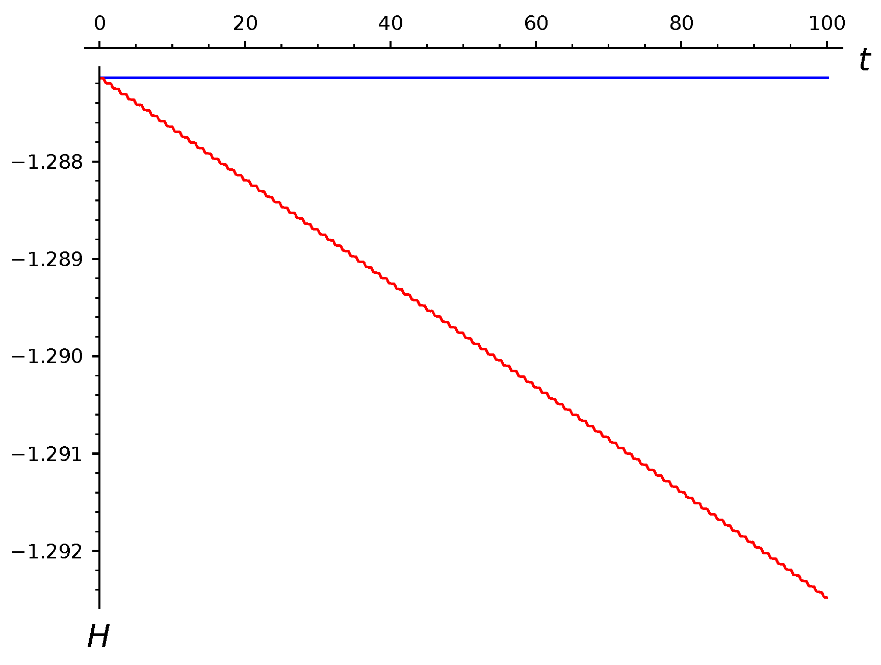
http://malykhmd.neocities.org (accessed on 8 December 2021). As is well known, in the solution found by the explicit fourth-order Runge–Kutta scheme, the energy
H changes and in a monotonic and noticeable way, as can be seen in
Figure 1. Thus, the change in energy was the center of our attention.
The midpoint scheme is implicit, so at each step, one has to solve a system of nonlinear equations. We used the simple iteration method with a fixed number of iterations and a step of
, which is approximately equal to
of the exact solution period [
35]. To eliminate the effect of round-off errors, we assigned
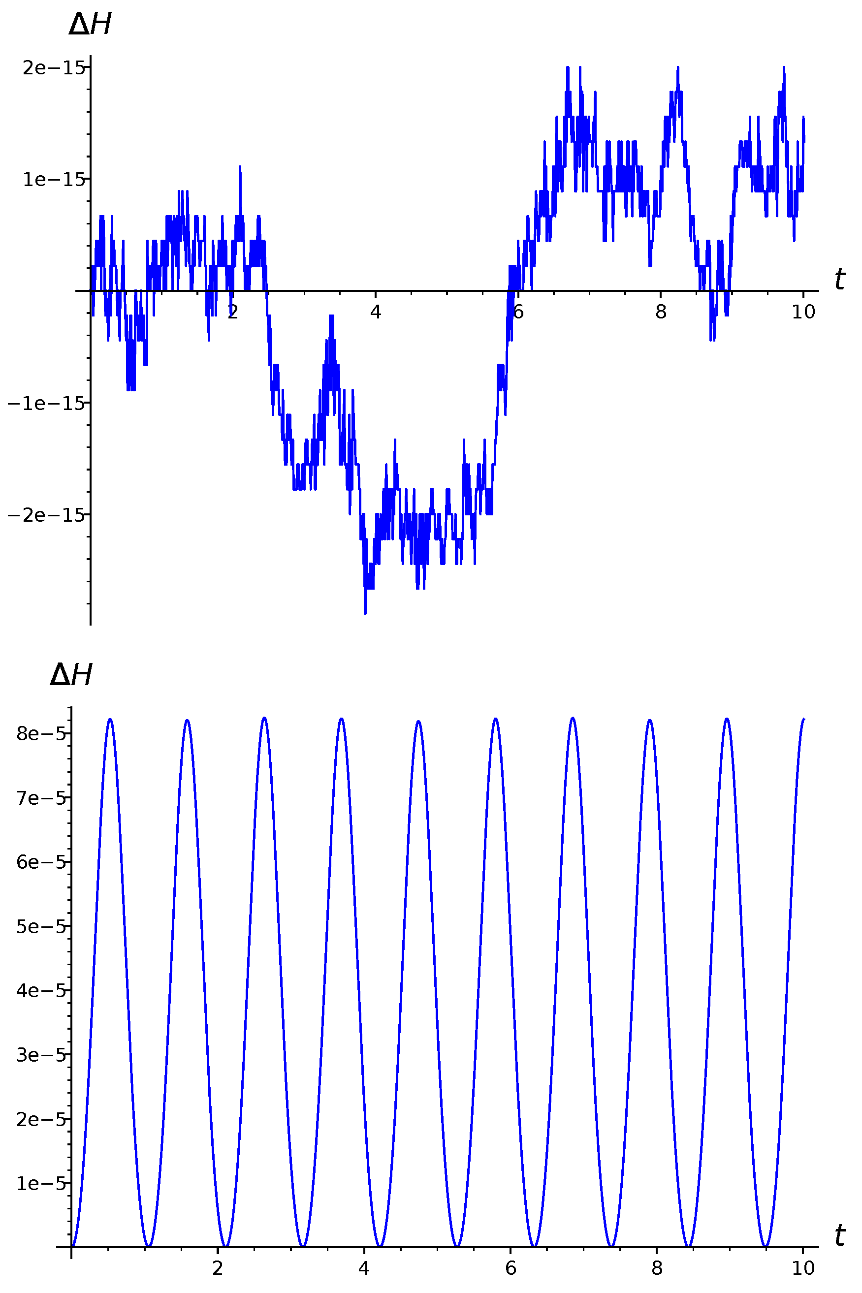
bits to decimals. As shown in
Figure 2, already at ten iterations, the energy increment is within the
limit. At the same time, in the solution found by the midpoint scheme without introducing additional variables, the energy fluctuates in the limit from 0 to
. Of course, we increased the number of iterations and made sure that the figures did not change. Thus, we did manage to modify the midpoint scheme so that energy was conserved.
6. Conclusions and Discussion
The major result of our work is Theorem 2: by introducing additional variables, the many-body problem can be reduced to a dynamical system with a rational right-hand side, all algebraic integrals of which are expressed in terms of quadratic and linear ones. Thus, both classical dynamical systems—the gyroscope rotation problem and the many-body problem—belong to the same type of dynamical systems. A natural application of this theorem is the possibility of constructing difference schemes of an arbitrary approximation order that exactly preserve all algebraic integrals on the basis of well-studied symplectic Runge–Kutta schemes.
The midpoint scheme is an example of such a scheme when it is applied to (10)–(13). It should be emphasized that, in this way, we can construct high-order schemes that preserve all integrals of motion in the many-body problem. The key problem with the application of these schemes in practice, of course, is their implicitness, which can be overcome by both numerical and numerical–analytical methods. Obviously, errors in solving a nonlinear system of algebraic equations describing one step in a scheme can completely level out all the advantages of the proposed scheme [
37]. Therefore, in our opinion, this issue requires further study, including numerical experiments. The numerical example given above is only intended to illustrate theoretical results.
However, we believe that the conservative difference schemes constructed above for the many-body problem will not only make it possible to carry out calculations for large times, but will also make it possible to qualitatively investigate the properties of solutions of the many-body problem by the finite difference method.
It should also be noted that when comparing the schemes, the focus of the researchers’ attention was always on the quantitative proximity of the exact and approximate solutions, while the question of preserving the qualitative properties of the exact solution remained insufficiently studied, although the tempting possibility to “determine the nature of the dynamic process using only rough calculations with a large grid pitch” according to the symplectic scheme was noted in [
38]. Meanwhile, for a linear oscillator, the simplest Runge–Kutta symplectic scheme, the midpoint scheme, allows not only the accurate preservation of the energy integral, but also to obtain an exact periodic approximate solution and closed polygons as an analogue of closed phase trajectories of the continuous model [
28].
In other words, after discretization, a model is obtained that inherits almost all the algebraic and qualitative properties of a continuous model. In the theory of partial differential equations, discretizations inheriting certain properties of differential equations and operations on the dependent variables included in them are called mimetic (i.e., imitative) or compatible [
39,
40]. Therefore, we find it appropriate to consider the construction of conservative difference schemes in the context of the more general and more important issue of constructing mimetic difference schemes for the many-body problem, of course, clarifying the concept itself.
We would like to refrain from predicting the usefulness of these schemes for the numerical integration of the many-body problem. It is important for us that the midpoint scheme gives a discrete model of the many-body problem that preserves all integrals. We plan to study its algebraic properties hoping to repeat the results obtained earlier for linear models [
28]. Lagrange’s case was considered in our talk at CASC’2020 [
41].


 ,
, 

