Bayesian Estimation of Adsorption and Desorption Parameters for Pore Scale Transport

Abstract

Stochastic parameter estimation and inversion have become increasingly popular in recent years. Nowadays, it is computationally reasonable and regular to solve complex inverse problems within the Bayesian framework. Applications of Bayesian inferences for inverse problems require investigation of the posterior distribution, which usually has a complex landscape and is highly dimensional. In these cases, Markov chain Monte Carlo methods (MCMC) are often used. This paper discusses a Bayesian approach for identifying adsorption and desorption rates in combination with a pore-scale reactive flow. Markov chain Monte Carlo sampling is used to estimate adsorption and desorption rates. The reactive transport in porous media is governed by incompressible Stokes equations, coupled with convection–diffusion equation for species’ transport. Adsorption and desorption are accounted via Robin boundary conditions. The Henry isotherm is considered for describing the reaction terms. The measured concentration at the outlet boundary is provided as additional information for the identification procedure. Metropolis–Hastings and Adaptive Metropolis algorithms are implemented. Credible intervals have been plotted from sampled posterior distributions for both algorithms. The impact of the noise in the measurements and influence of several measurements for Bayesian identification procedure is studied. Sample analysis using the autocorrelation function and acceptance rate is performed to estimate mixing of the Markov chain. As result, we conclude that MCMC sampling algorithm within the Bayesian framework is good enough to determine an admissible set of parameters via credible intervals.

1. Introduction

Reactive transport in porous media is important for many industrial and environmental applications such as water treatment, soil contamination and remediation, catalytic filters, etc. Most of the experimental and theoretical studies of porous media transport and reactive transport have been carried out on the macroscopic Darcy scale [1,2]. In many instances, the weak point in the computational modeling of reactive transport is the lack of data on the rate of adsorption and desorption at the pore scale (or, more generally, the parameters of heterogeneous reactions). Despite the progress in the development of devices for making experimental observations at the pore scale, the experimental determination of these rates is still quite difficult.

In the case of surface (heterogeneous) reactions at the pore scale, the species’ transport is coupled to surface reaction via Robin boundary conditions. When the reaction rates are not known, their identification belongs to the class of inverse boundary value problems [3,4,5,6]. The additional information that is needed to identify these parameters is often provided in the form of dynamic data related to the concentration at the outlet (e.g., so called breakthrough curves). Different algorithms can be applied for solving parameter identification problems, see, e.g., [7,8]. The main idea behind parameter identification is to find these parameters for which the model predictions best match our measurements or observations in a real physical system. Many algorithms use deterministic methods based on Tikhonov’s regularization method [9,10]. There are algorithms using a stochastic approach such as Pure Random Search [11]. However, any approach that gives only one best value for the parameter vector does not take into account the fact that our measurements contain measurement noise. In other words, deterministic inversion methods do not account for the uncertainty in parameter estimates.

Uncertainty quantification (UQ) is an important area of research in many applications. All experimental data have regular errors arising from instruments or human operators. This leads to a shift in the parameters of the fitted empirical model [12,13]. In our applications, besides measurement errors, we deal with model errors. The measured data show an integrated response, which averages the information related to pore-scale geometries. In our simulations, we use a specific pore-scale geometry which can differ from the real geometry. Thus, including errors in the measurement is important.

The commonly used method for UQ is a Bayesian inversion, which formulates the posterior distribution via likelihood and prior information. In the paper, uninformative prior distribution for the parameters is used. For the likelihood, we use the error in the average concentration at the outlet. In particular, we use the $L^2$ difference between the average concentration at the outlet and the observed data. The likelihood function involves solving forward PDE model, which can be expensive due to complex pore-scale geometries. Consequently, the evaluation of the likelihood is expensive. For sampling from the posterior distribution, the Markov chain Monte-Carlo methods (MCMC) is used [14,15,16,17]. Sampling the posterior distribution is the major computational difficulty associated with Bayesian inversion. MCMC—an increasingly popular method of obtaining information on distribution, especially for the evaluation of posterior distributions in Bayesian inference [18]. Areas in which this approach works well include dynamic systems models in ecology, geophysics, chemical kinetics, signal detection theory and decision theory [19,20,21].

In our previous works on reactive flows [22,23] a deterministic approach was considered, where the parameter space was divided into a uniform grid, where for each point the direct problem was solved to construct the residual functional. This approach was one of the simplest, but depending on the functionality, a denser mesh partition may be required, which could lead to a large amount of computation. Furthermore, research was done on stochastic approaches, where points were taken at random in the parameter space. The good thing about this approach was that it was quite cheap compared to the deterministic approach to evaluate the functionality of the residual, but this approach was more useful as a preliminary exercise to reduce the search space. In connection with these results, it was decided to continue the work and consider other approaches for identifying the parameters of the rates of surface reactions.

In this paper, we will discuss the determination of reaction rates, namely adsorption and desorption parameters for pore scale transport in porous media using MCMC sampling within the framework of Bayesian inference. This method provides the ability not only to identify parameters, but also to quantify uncertainty. The reactive transport is governed by incompressible Stokes equations in pore-scale geometry, coupled with a convection–diffusion equation for species transport. The surface reactions are accounted via Robin boundary conditions. The Henry isotherm is considered for correct description of the reaction dynamics at the solid–fluid interface. The main feature of this problem is a nonlinear boundary condition for surface concentration of adsorbed solute on obstacles surface. Finite element method (FEM) is exploited. The family of MCMC methods, namely Metropolis–Hastings and Adaptive Metropolis algorithms was implemented. Sample analysis using autocorrelation function and acceptance rate is performed to estimate mixing of the Markov chain. Credible intervals have been plotted from sampled posterior distributions for both algorithms. The impact of the noise in the measurements and influence of several measurements for Bayesian inversion procedure is studied.

The remainder of the paper is organized as follows. Section 2 formulates a mathematical model of reactive flow in porous media. In Section 3, we consider the Bayesian statement of the problem. In Section 4, we observe MCMC sampling techniques. In Section 5, we provide an estimate of the parameters based on sample data. Finally, Section 6 summarizes the results presented in this paper.

2. Forward Problem

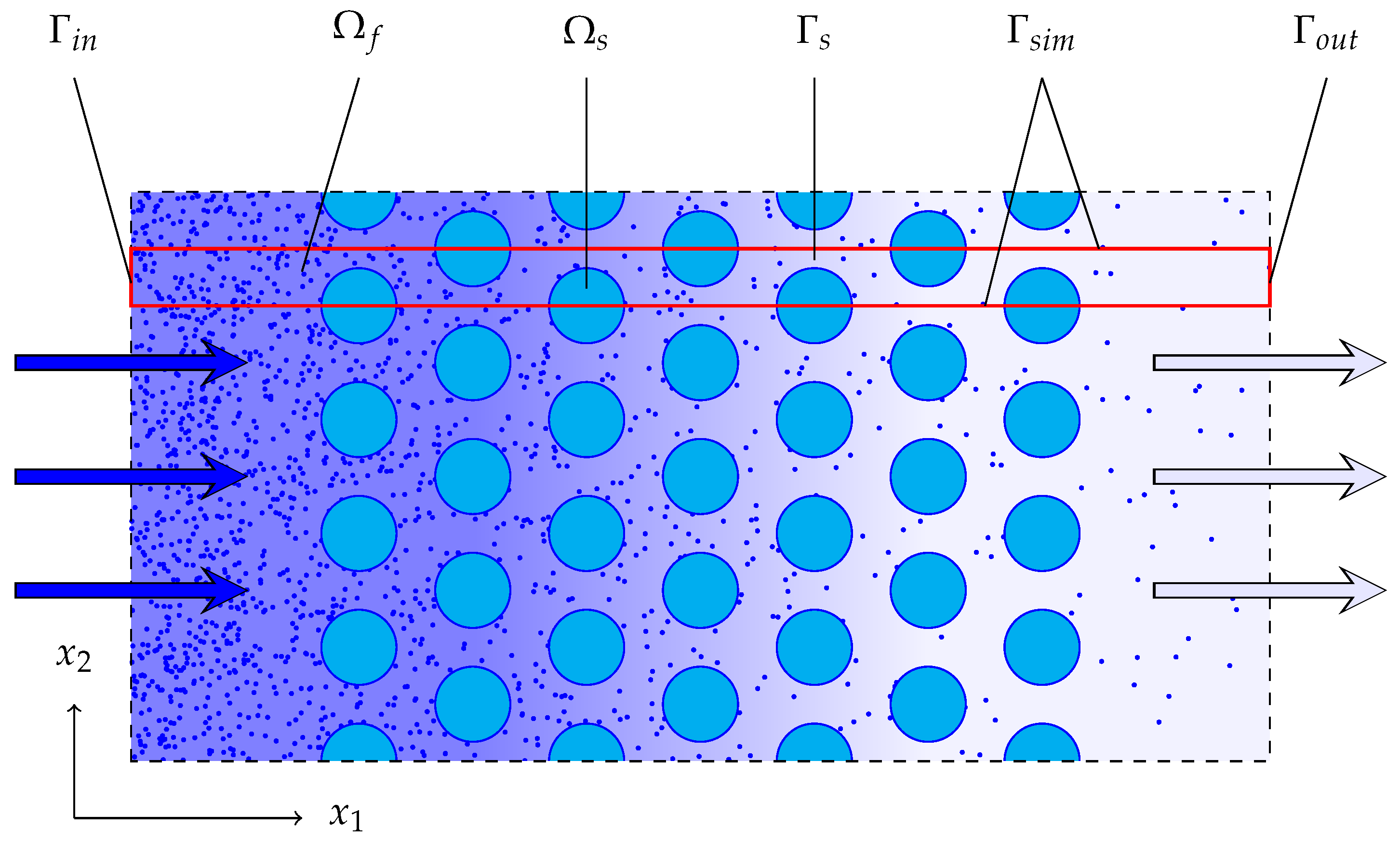
Two dimensional transport of a dissolved substance is considered at pore scale in the presence of heterogeneous reactions. Periodic porous media geometry is considered here, see Figure 1. The computational domain ${\Omega }_f$ is occupied by a fluid. The reaction occurs at the surface of the obstacles, the latter is denoted by ${\Gamma }_s$. Symmetry boundary conditions are assigned at the top and the bottom boundary ${\Gamma }_{sim}$. The inlet boundary is denoted by ${\Gamma }_{in}$, and the outlet is denoted by ${\Gamma }_{out}$. Coupled incompressible Stokes equations and convection–diffusion equations for species transport are governing the reactive transport. Adsorption and desorption are accounted via Robin boundary conditions. The dimensionless form of the governing equations is used in this paper.

This problem that has already been investigated by us in our previous works [22,23] in conjunction with deterministic methods for parameter identification, but for the completeness of the presentation we describe here it again.

The IBVP is discretized in space by Finite Element Method (FEM), and implicit discretization in time is used. The computations are performed using the FEniCS PDE computing platform [24].

2.1. System of Equations

Steady state incompressible Stokes equations are governing the flow:

$$\nabla p-\mu {\nabla }^2\mathit{u}=0,$$

(1)

$$\nabla ·\mathit{u}=0,\hspace{1em}\mathit{x}\in {\Omega }_f,$$

(2)

where $\mathit{u}\left(\mathit{x}\right)$ and $p\left(\mathit{x}\right)$ are the fluid velocity and pressure, respectively, and $\mu >0$ is the viscosity, which we consider constant [1,25].

The notation $c(\mathit{x},t)$ stands for the concentration of the solute in the fluid. The unsteady transfer of solute in the absence of homogeneous reactions is described by the convection–diffusion equation

$$\frac{\partial c}{\partial t}+\nabla \left(\mathit{u}c\right)-D{\nabla }^{2}c=0,\hspace{1em}\mathit{x}\in {\Omega }_f,\hspace{1em}t>0,$$

(3)

Here, $D>0$ stands for the diffusion coefficient of a solute, which is assumed to be constant and scalar.

Mass conservation is used to specify the interface conditions at the reactive surface ${\Gamma }_s$. Namely, the change in the adsorbed surface concentration is equal to the flux from the fluid to the surface. Thus

$$\frac{\partial m}{\partial t}=-D\nabla c·\mathit{n},\hspace{1em}\mathit{x}\in {\Gamma }_s,$$

(4)

where m is the concentration of adsorbed solute on the surface [26]. A mixed kinetic–diffusion description of adsorption is used:

$$\frac{\partial m}{\partial t}=f(c,m).$$

(5)

The choice of f and its dependence on c and m is depend on the particular reaction dynamics. There are a number of different isotherms (i.e., different functions $f(c,m)$) to describe these dynamics. The Henry isotherm, which assumes a linear relationship between the near surface concentration and the surface concentration of the adsorbed particles, is the simplest one. It is specified as

$$f(c,m)=k_{a}c-k_{d}m,$$

(6)

where $k_a\ge 0$ is the rate of adsorption, measured in unit length per unit time, and $k_d\ge 0$ is the rate of desorption, measured per unit time.

2.2. Boundary and Initial Conditions

Let us denote by $\mathit{n}$ the outer normal vector to the boundary. Boundary conditions on $\partial {\Omega }_f$ are specified as follows. The velocity of the fluid $\overline{u}$ is prescribed at the inlet

$$\mathit{u}·\mathit{n}=\overline{u},\hspace{1em}\mathit{u}\times \mathit{n}=0,\hspace{1em}\mathit{x}\in {\Gamma }_{in}.$$

(7)

Standard conditions are prescribed at the outlet, namely, pressure and absence of tangential force

$$p-\mathbf{\sigma }\mathit{n}·\mathit{n}=\overline{p},\hspace{1em}\mathbf{\sigma }\mathit{n}\times \mathit{n}=0,\hspace{1em}\mathit{x}\in {\Gamma }_{out}.$$

(8)

Standard no-slip and no-penetration conditions are prescribed on the obstacles surface:

$$\mathit{u}·\mathit{n}=0,\hspace{1em}\mathit{u}\times \mathit{n}=0,\hspace{1em}\mathit{x}\in {\Gamma }_s.$$

(9)

Symmetry conditions are assigned on the symmetry boundary:

$$\mathit{u}·\mathit{n}=0,\hspace{1em}\mathbf{\sigma }\mathit{n}\times \mathit{n}=0,\hspace{1em}\mathit{x}\in {\Gamma }_{sim}.$$

(10)

The concentration of the solute at the inlet is specified as follows:

$$c(\mathit{x},t)=\overline{c},\hspace{1em}\mathit{x}\in {\Gamma }_{in},$$

(11)

where $\overline{c}>0$ is assumed to be constant. On the external boundaries and at the outlet zero diffusive flux is prescribed:

$$D\nabla c·\mathit{n}=0,\hspace{1em}\mathit{x}\in {\Gamma }_{sim}\cup {\Gamma }_{out}.$$

(12)

Convective flux through the outlet is implicitly allowed by the above equations.

Initial conditions need to be specified to complete the formulation of the IBVP, in addition to the governing Equations (3) and (5), boundary conditions (7)–(12), and specified isotherm (6),

$$c(\mathit{x},0)=c_0\left(\mathit{x}\right),\hspace{1em}\mathit{x}\in {\Omega }_f,$$

(13)

$$m(\mathit{x},0)=m_0\left(\mathit{x}\right),\hspace{1em}\mathit{x}\in {\Gamma }_s.$$

(14)

2.3. Dimensionless Form of the Equations

The same notations are used for the dimensionless variables (velocity, pressure, concentration). The height of the computational domain ${\Omega }_f$, namely l, is used for scaling spatial sizes, the scaling of the concentration is done by the inlet concentration $\overline{c}$ and the scaling of the velocity is done by the inlet velocity $\overline{u}$.

Assuming the dimensionless viscosity to be equal to unity, the Stokes Equations (1) and (2) and its boundary conditions in dimensionless remain are written as

In dimensionless form (3) reads

$$\frac{\partial c}{\partial t}+\nabla \left(\mathit{u}c\right)-\frac{1}{\mathrm{Pe}}{\nabla }^{2}c=0,\hspace{1em}\mathit{x}\in {\Omega }_f,\hspace{1em}t>0,$$

(15)

where

$$\mathrm{Pe}=\frac{l\overline{u}}{D}$$

is the Peclet number.

Next, (11) turns into

$$c=1,\hspace{1em}\mathit{x}\in {\Gamma }_{in},$$

(16)

where the boundary condition (12) takes the form

$$\nabla c·\mathit{n}=0,\hspace{1em}\mathit{x}\in {\Gamma }_{sim}\cup {\Gamma }_{out}.$$

(17)

The dimensionless form of (4) is given by

$$\frac{\partial m}{\partial t}=-\nabla c·\mathit{n},\hspace{1em}\mathit{x}\in {\Gamma }_s.$$

(18)

In dimensionless form the interface reaction is described as

$$\frac{\partial m}{\partial t}={\mathrm{Da}}_{a}c-{\mathrm{Da}}_{d}m,\hspace{1em}\mathit{x}\in {\Gamma }_s,$$

(19)

here the Damköler numbers for adsorption and desorption are given by following:

$${\mathrm{Da}}_a=\frac{k_a}{\overline{u}},\hspace{1em}{\mathrm{Da}}_d=\frac{k_{d}l}{\overline{u}}.$$

2.4. Variational Formulation

Note that the fluid flow influences the species transport, however the species concentration does not influence the fluid flow. Due to this, the flow can be computed only once in advance. The FEM approximation of the steady state flow problem [27] is based on variational formulation of the considered boundary value problem (1)–(10). The following functional space $\mathit{V}$ is defined for the velocity $\mathit{u}$ ($\mathit{u}\in \mathit{V}$):

$$\begin{array}{cc}\hfill \mathit{V}=\{\mathit{u}\in {\mathit{H}}^1(\Omega ):& \mathit{u}·\mathit{n}=1, \mathit{u}\times \mathit{n}=0 \mathrm{on} {\Gamma }_{in},\hfill \\ & \mathit{u}=0 \mathrm{on} {\Gamma }_s, \mathit{u}·\mathit{n}=0 \mathrm{on} {\Gamma }_{sim}\}.\hfill \end{array}$$

Test function $\mathit{v}s.\in \widehat{\mathit{V}}$, where

$$\widehat{\mathit{V}}=\{\mathit{v}s.\in {\mathit{H}}^1\left({\Omega }_f\right): \mathit{v}=0 \mathrm{on} {\Gamma }_{in}, \mathit{v}=0 \mathrm{on} {\Gamma }_s, \mathit{v}·\mathit{n}=0 \mathrm{on} {\Gamma }_{sim}\}.$$

For the pressure p and the related test functions q, it is required that $p,q\in Q$, where

$$Q=\{q\in L_2\left({\Omega }_f\right): q=0 \mathrm{on} {\Gamma }_{out}\}.$$

Multiplying (1) by $\mathit{v}$, (2) by q, integrating over the computational domain and taking into account the boundary conditions (7)–(10), the following system of equations is obtained with respect to $\mathit{v}s.\in \mathit{V}$, $p\in Q$

$$a(\mathit{u},\mathit{v})-b(\mathit{v},p)=0 \forall \mathit{v}s.\in \widehat{\mathit{V}},$$

(20)

$$b(\mathit{u},q)=0 \forall q\in Q.$$

(21)

Here

$$a(\mathit{u},\mathit{v}):={\int }_{{\Omega }_f}\nabla \mathit{u}·\nabla \mathit{v}s. d\mathit{x},$$

$$b(\mathit{v},q):={\int }_{{\Omega }_f}(\nabla ·\mathit{v})q d\mathit{x}.$$

The following finite dimensional subspaces are used for the basis and test functions in the FEM approximation of the velocity and the pressure: ${\mathit{V}}_h\subset \mathit{V}$, ${\widehat{\mathit{V}}}_h\subset \widehat{\mathit{V}}$ and $Q_h\subset Q$.

The unsteady species transport problem (15)–(19) is solved numerically using finite elements. Here we define

$$S=\{c\in H^1\left({\Omega }_f\right): c=1 \mathrm{on} {\Gamma }_{in}\},$$

$$\widehat{S}=\{s\in H^1\left({\Omega }_f\right): s=0 \mathrm{on} {\Gamma }_{in}\}.$$

The approximate solution $c\in S$ is sought from

$$\left(\frac{\partial c}{\partial t},s\right)+d(c,s)={\left(\frac{\partial m}{\partial t},s\right)}_s\hspace{1em}\forall s\in \widehat{S},$$

(22)

where the following notations are used

$$d(c,s):=-{\int }_{{\Omega }_f}c\mathit{u}·\nabla s d\mathit{x}+\frac{1}{\mathrm{Pe}}{\int }_{{\Omega }_f}\nabla c·\nabla s d\mathit{x}+{\int }_{{\Gamma }_{out}}(\mathit{u}·\mathit{n})cs d\mathit{x},$$

$${(\phi ,s)}_s:=-{\int }_{{\Gamma }_s}\phi s d\mathit{x}.$$

For determining $m\in G=L_2\left({\Gamma }_s\right)$ (see (5)) we use

$${\left(\frac{\partial m}{\partial t},g\right)}_s-{(f(c,m),g)}_s=0,\hspace{1em}g\in G.$$

(23)

Symmetric Crank–Nicolson discretization method is used for time discretization (see, e.g., [28,29]). Let $\tau$ be a step-size of a uniform grid in time such that $c^n=c\left(t^n\right)$, $t^n=n\tau , n=0,1,...$.

Equation (22) is approximated in time as follows

$$\left(\frac{c^{n+1}-c^n}{\tau },s\right)+d\left(\frac{c^{n+1}+c^n}{2},s\right)={\left(\frac{m^{n+1}-m^n}{\tau },s\right)}_s.$$

In a similar way for (23) we get

$${\left(\frac{m^{n+1}-m^n}{\tau },g\right)}_s-{\left(f\left(\frac{c^{n+1}+c^n}{2},\frac{m^{n+1}+m^n}{2}\right),g\right)}_s=0,\hspace{1em}n=0,1,\dots ,$$

Zero initial conditions are posed in the considered here case,

$$c^0=0,\hspace{1em}\mathit{x}\in {\Omega }_f,$$

$$m^0=0,\hspace{1em}\mathit{x}\in {\Gamma }_s.$$

2.5. Numerical Solution of the Forward Problem

Small pure fluid regions are added in front of the inlet and behind the outlet, as it is usual for pore scale simulations. The computational domain $\Omega$ is triangulated using the mesh generator software Gmsh [30]. In order to control the accuracy of results, computations on consecutively refined grids were performed on our previous work [23].

Taylor–Hood $P_2-P_1$ elements [31] are selected in solving Stokes equations. These are continuous $P_2$ and $P_1$ Lagrange elements for the velocity components and for the pressure field, respectively. The computations are performed using the PDE framework FEniCS [24,32].

The unsteady species transport problem (15), (18) and (19) is solved numerically using standard Lagrangian $P_1$ finite elements. For details on the FE discretization, see [33].

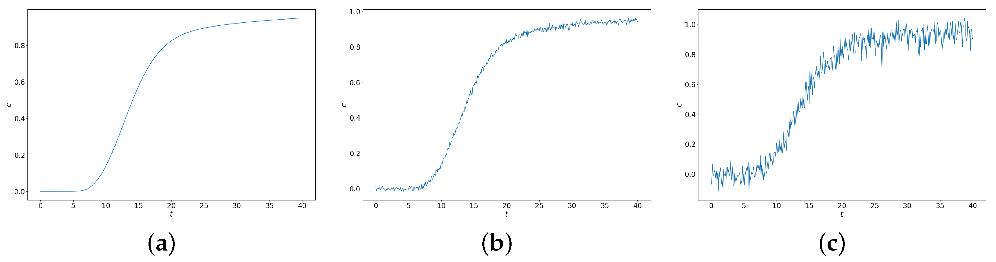
Sensitivity studies are performed first to evaluate the influence of the grid parameters on the accuracy. The basic set of parameters reads as follows:

$$\mathrm{Pe}=10, {\mathrm{Da}}_a=0.005, {\mathrm{Da}}_d=0.05.$$

The non-stationary problem is solved on dimensionless time interval $(0,T)$, $T=40$, with a time step $\tau =0.1$. Breakthrough curve (i.e., time dependent average outlet concentration) is used to characterize the reactive transport:

$$c_{out}\left(t\right)=\frac{{\int }_{{\Gamma }_{out}}c(\mathit{x},t)d\mathit{x}}{{\int }_{{\Gamma }_{out}}d\mathit{x}}.$$

(24)

The breakthrough curve for these parameters is shown in Figure 2a.

Detailed results of solving the direct problem can be found in our previous work [23].

3. Inverse Problem

Experimental measurements can have systematic errors due to the quality of the instruments or due to human factors. Thus, this can lead to a shift in the parameters of the fitted empirical model. Random errors in experimental data, especially with a small dataset, also affect models, since the extremum of the functional will shift depending on the variance of the noise. All sensors that are used to collect data also have the form of model and uncertainty. Thus, it is extremely important to take into account the influence of these uncertainties in inverse problems. To solve this problem, we will use a Bayesian approach [34,35], which will help us not only to identify the parameters, but also quantify associated uncertainty. A term called credible interval [36] will be used for this.

3.1. Experimental Measurements

The aim of this work is to determine the rates of adsorption and desorption based on synthetic experimental measurements $\mathit{d}$ given by:

$$\mathit{d}=\mathit{f}\left(\mathbf{\theta }\right)+\mathbf{\epsilon },$$

(25)

where $\mathit{f}\left(\mathbf{\theta }\right)$ is breakthrough curve (24), obtained by solving the forward problem described in the previous section using the following vector of parameters $\mathbf{\theta }=\{{\mathrm{Da}}_a,{\mathrm{Da}}_d\}$, $\mathbf{\epsilon }$. The latter is additional noise which has Gaussian distribution $\mathcal{N}(0,{\sigma }^2)$ with zero mean and variance ${\sigma }^2$. This kind of noise is also known as “White noise” [37]. Experimental measurements with different variances of the noise can be seen in Figure 2b,c.

3.2. Bayesian Inversion Approach

The Bayesian formulation poses the parameter estimation problem as a problem of statistical inference over parameter space. The solution of the resulting Bayesian inverse problem is a posterior probability density function (PDF) [13,34,35,36]. Bayes’ Theorem states the posterior PDF explicitly as

$$\rho \left(\mathbf{\theta }\right|\mathit{d})\propto \rho (\mathit{d}\left|\mathbf{\theta }\right)\rho \left(\mathbf{\theta }\right),$$

(26)

where $\rho \left(\mathit{d}\right|\mathbf{\theta })$—likelihood function, $\rho \left(\mathbf{\theta }\right)$—prior knowledge about parameters.

If the variance of the noise is assumed to be known, since the noise $\mathbf{\epsilon }$ is independent from $\mathbf{\theta }$, the likelihood function takes a simple multi-Gaussian form

$$\rho \left(\mathit{d}\right|\mathbf{\theta })=\frac{1}{{\left(2\pi {\sigma }^2\right)}^{N/2}}\prod _{i=1}^N\exp \left(-\frac{1}{2{\sigma }^2}{\Vert {\mathit{d}}_i-\mathit{f}\left(\mathbf{\theta }\right)\Vert }^2\right),$$

(27)

where N is the number of measurements.

At least some information about the sought parameters should be specified in advance. For example, positive, range based on the considered physical problem, etc. For the situation with a very limited information, the best way is to choose uniform priors. By uniform prior we mean that parameters in the range [0, 0.01] for ${\mathrm{Da}}_a$ and [0, 0.1] for ${\mathrm{Da}}_d$ are equally likely to be desired parameter. In some of the literature, this prior is called non-informative prior or flat prior, i.e., $\rho \left(\mathbf{\theta }\right)\propto 1$ over the region of interest. In this case our posterior will be proportional to our likelihood distribution

$$\rho \left(\mathbf{\theta }\right|\mathit{d})\propto \rho (\mathit{d}\left|\mathbf{\theta }\right).$$

(28)

4. Markov Chain Monte-Carlo

MCMC is a computer-driven method that allows to represent a distribution by randomly sampling values from the distribution, without knowing all mathematical properties [38,39]. The MCMC method has a fairly simple concept and in order to apply this method, it is enough to know how to calculate the density for different samples. The name MCMC fuses two properties: Monte-Carlo and Markov chain. Monte-Carlo is the practice of evaluating the properties of a distribution by extracting random samples from the distribution. As an example, instead of finding the mean of the normal distribution by calculating it directly from the distribution’s equations, the Monte Carlo approach would be to extract a large number of random samples from the normal distribution and calculate their mean. The advantage of the Monte Carlo method is clear: calculating the mean over a large sample of numbers can be much easier than calculating the mean directly from the normal distribution’s equations. This advantage is most evident when random samples are easy to draw and distribution’s equations are difficult to work with in other ways. The property of a Markov chain is that random samples are generated using a special rule: the creation of a new random sample depends only on the current sample, hence the name—chain. A special property of the chain is that, although each new sample depends on the previous one, the new samples do not depend on any samples before the previous one, this is the Markov property. MCMC is especially useful in Bayesian inference because of its emphasis on posterior distributions, which are often difficult to work with analytically. MCMC allows the user to approximate aspects of the posterior distribution that cannot be calculated directly [18]. The Markov chain constructed by this method in its stationary distribution will approximate the desired distribution.

4.1. Metropolis–Hastings Algorithm

The most popular MCMC method is probably the Metropolis–Hasting (MH) algorithm. MH enables us to obtain samples from any probability distribution, $\rho \left(\mathbf{\theta }\right)$, given that we can compute at least a value proportional to it, hence ignoring the normalization factor. This is very useful because in a lot of problems, the hard part is to compute the normalization factor, especially in large dimensions.

The MH algorithm reads as follows:

• Choose an initial value for a parameter, ${\mathbf{\theta }}_i$. This can be done randomly or by making an educated guess.
• Choose a new parameter value, ${\mathbf{\theta }}_{i+1}$, by sampling from an easy-to-sample distribution, such as a Gaussian or uniform distribution, $q\left({\mathbf{\theta }}_{i+1}\right|{\mathbf{\theta }}_i)$. We can think of this step as perturbing the ${\mathbf{\theta }}_i$ state somehow.
• Compute the probability of accepting a new parameter value by using the Metropolis–Hastings criterion:

  $${\rho }_a\left({\mathbf{\theta }}_{i+1}\right|{\mathbf{\theta }}_i)=min\left(1,\frac{\rho \left({\mathbf{\theta }}_{i+1}\right)q\left({\mathbf{\theta }}_i\right|{\mathbf{\theta }}_{i+1})}{\rho \left({\mathbf{\theta }}_i\right)q\left({\mathbf{\theta }}_{i+1}\right|{\mathbf{\theta }}_i)}\right)$$

  (29)
• If the probability computed on step 3 is larger than the value taken from a uniform distribution on the [0, 1] interval, we accept the new state; otherwise, we stay in the old state.
• We iterate from step 2 until we have enough samples.

4.2. Adaptive Metropolis Algorithm

The weak point of the MCMC in general and MH in particular is that they require a proposal that fits the target distribution, so the sampling was efficient. Finding such proposal can be very time consuming and therefore expensive process because, requires adjustment by trial and error. Naturally, there were developed various algorithms to adjust the proposals in the run-time adaptively [40]. One of the simplest adaptive algorithms, which was chosen in this work as an alternative to the MH algorithm, is the Adaptive Metropolis (AM) algorithm [41], which calculates the covariance matrix of the resulting chain and uses it as a proposal. In the AM algorithm, a new point does not depend only on the previous point, it depends on all previously selected points, thus, it loses the Markov property, but nevertheless, if the adaptation is based on an increasing part of the chain, it can be proved that the algorithm gives the correct ergodic result.

Adaptive Metropolis is a random walk algorithm that uses Gaussian proposal with a covariance that depend on the chain generated so far,

$$C_n=\left\{\begin{array}{cc}{C}_0,& n\le n_0,\\ s_d cov({\theta }_1,...,{\theta }_n)+s_d\epsilon I_d,& n>n_0,\end{array}\right.$$

(30)

where $s_d$ is a scaling parameter which taken as $s_d=2.4^2/d$ and depends only on the dimension d of the sampling space, $\epsilon >0$ is a constant that we can choose very small, $I_d$ is the d—dimensional identity matrix, and $n_0>0$, defines the length of the initial non-adaptation period.

The choice of the length of the initial non-adaptive part of the simulation, $n_0$, is free. It is not necessary to update the covariance every step, this can be done every $n_0$th step only using the entire history. This adaptation method improves the mixing properties of the algorithm, thereby increasing the simulation efficiency, which is commonly good for large dimensions. In this work, $n_0$ was chosen equal to 30. The role of the parameter $\epsilon$ is to ensure that $C_n$ will not become singular. In practical computations $\epsilon$ can be safely set to zero. The initial covariance $C_0$ should be strictly positive definite matrix and must move chain sufficiently [41]. The algorithm is exactly the same as in the MH algorithm, with the exception of proposal, which is given as a Gaussian distribution with mean ${\theta }_n$ and covariance (30). Additionally, the item is added, that the covariance matrix must be updated every $n_0$th step using the entire history.

Roberts et al. [42] proved that for $d\to \infty$, the asymptotically optimal acceptance rate is 0.234. This is a significant refinement of the general principle, where the acceptance rate must necessarily be far from 0 and far from 1.

5. Results

Bayesian estimation using MCMC sampling for identification of adsorption and desorption rates are performed in combination with reactive flow considered at the pore-scale. The reactive transport is governed by incompressible Stokes equations, coupled with convection–diffusion equation for species’ transport. Adsorption and desorption are accounted via Robin boundary conditions. The Henry isotherm is considered for describing the reaction terms. Synthetic experimental measurements of concentration at the outlet of the domain is provided to carry out the identification procedure. Metropolis–Hastings and Adaptive Metropolis algorithms are implemented.

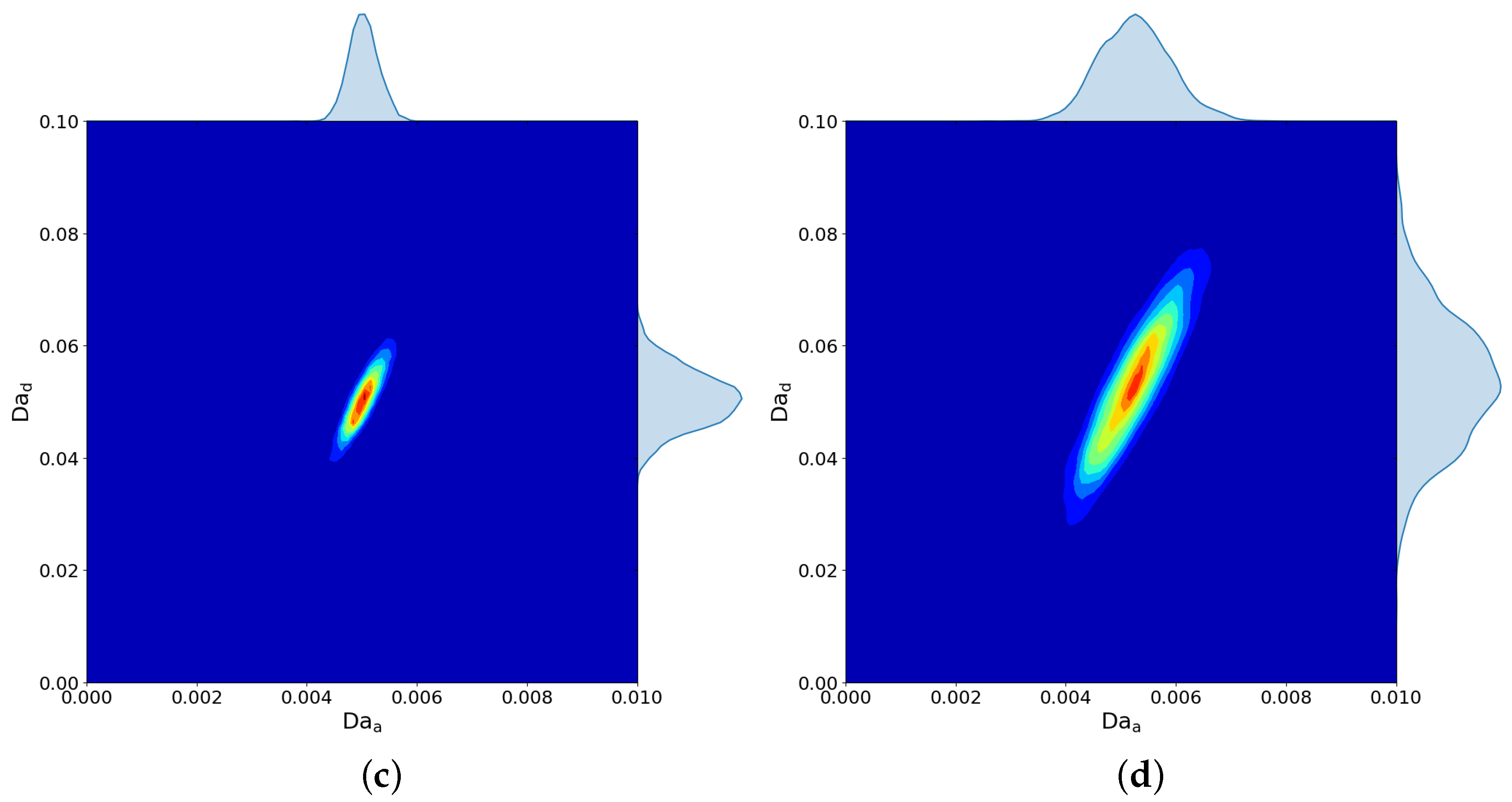
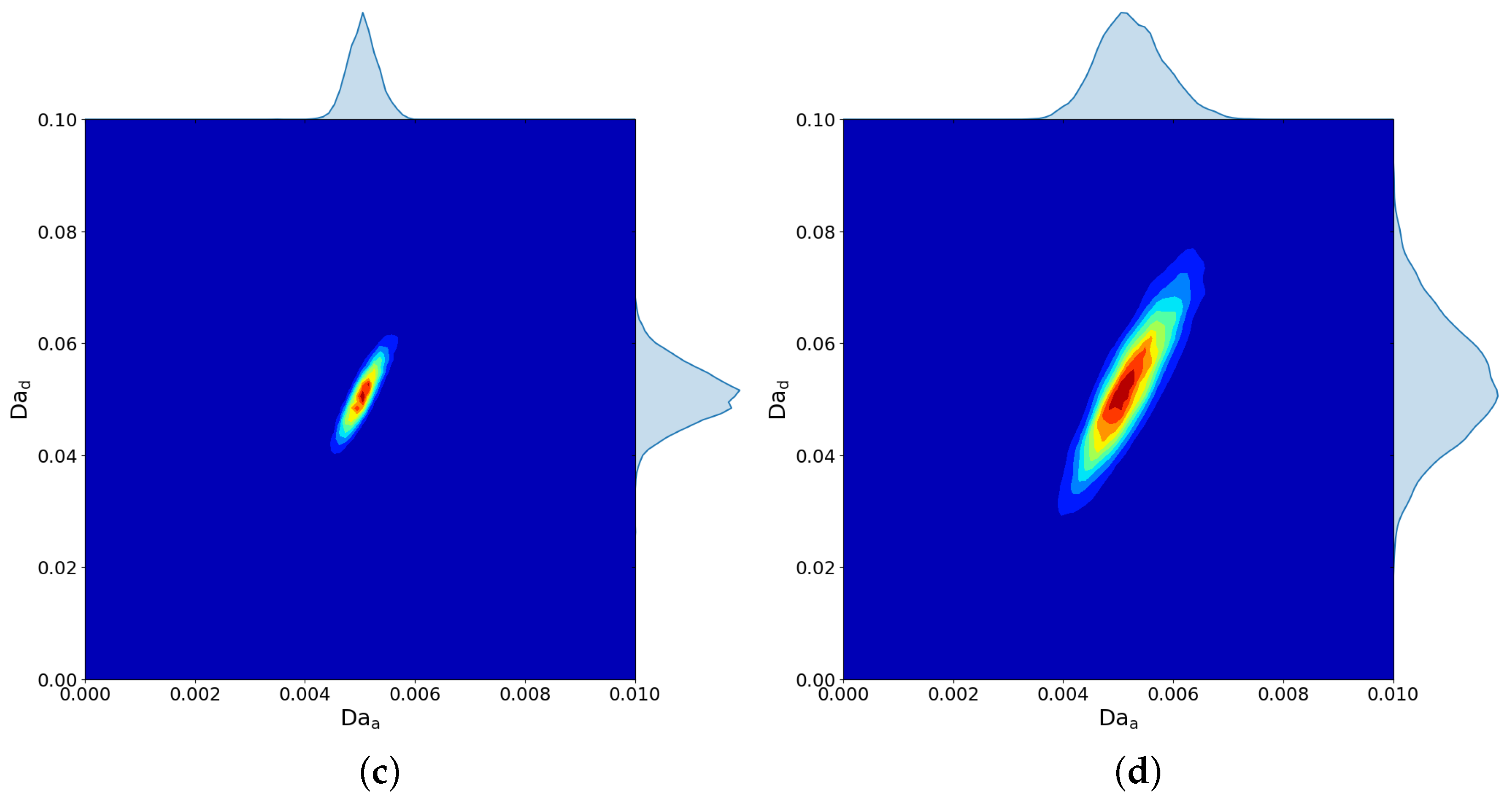
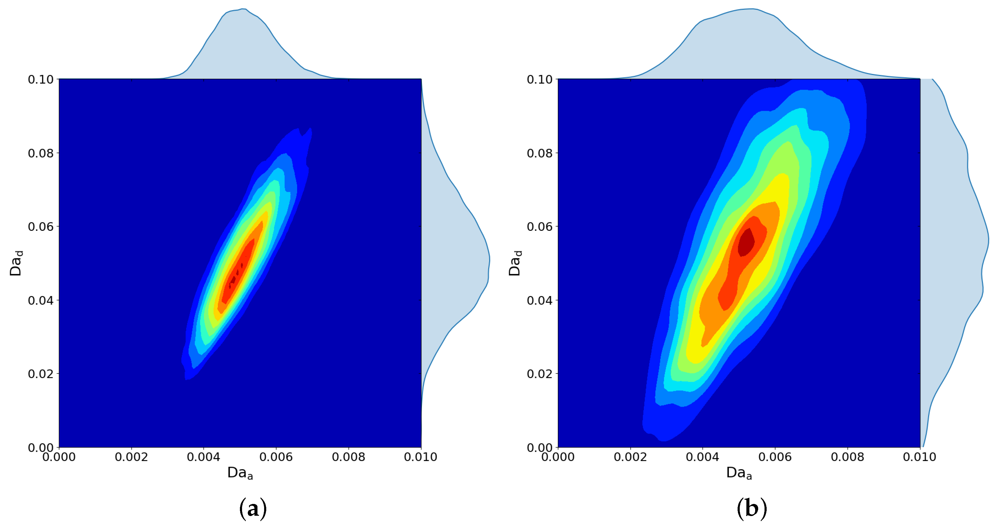
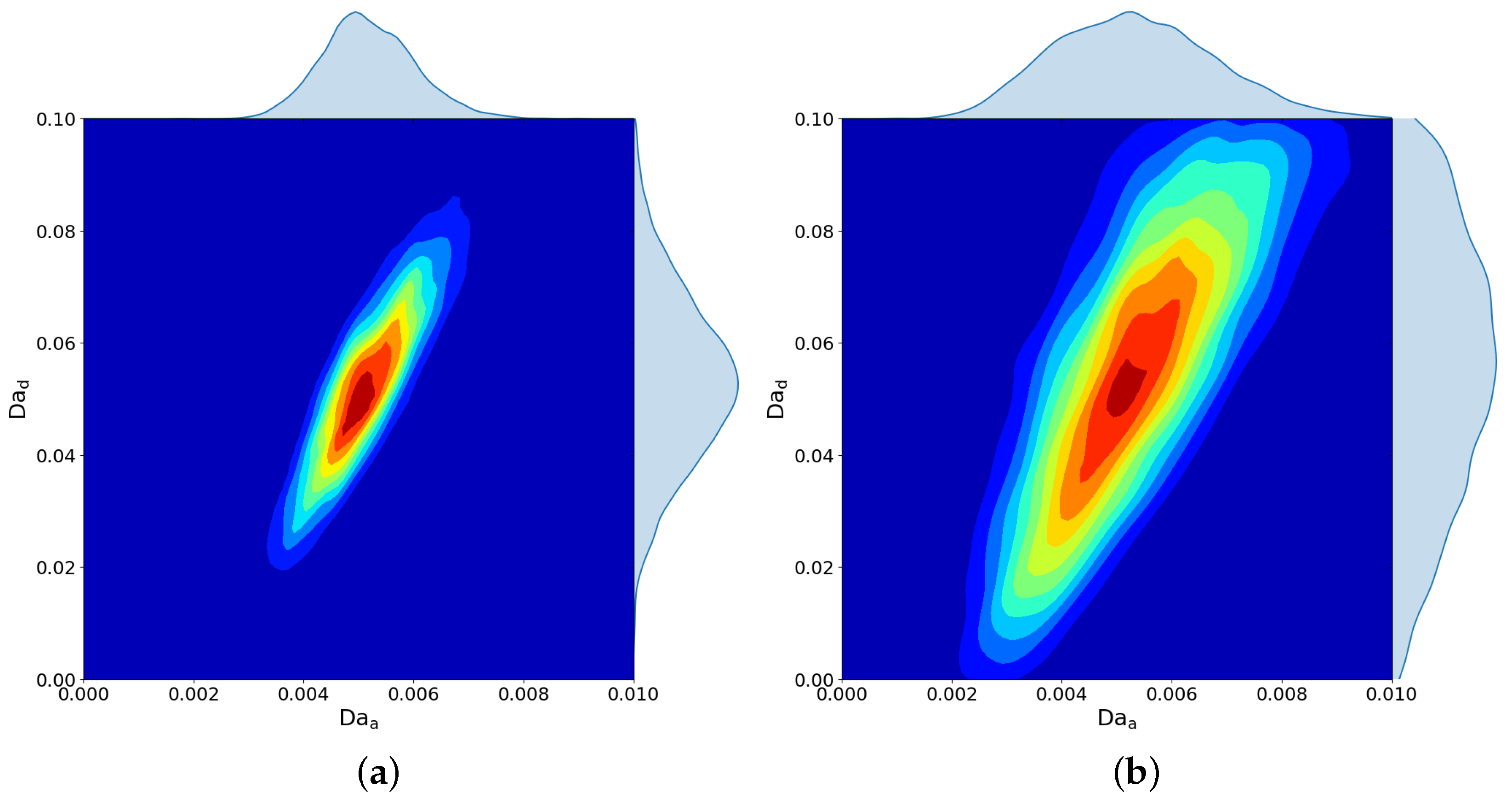
Figure 3 and Figure 4 clearly show that the higher noise amplitude leads to higher uncertainty and the larger count of observation data leads to more accurate parameter estimate. Results of MH is presented in Figure 3 and AM is presented in Figure 4. As we can see, the results quite similar and AM results are obtained without the time-consuming trial–error proposal tuning procedure as in the MH algorithm.

Table 1. True values: ${\mathrm{Da}}_a=0.005$, ${\mathrm{Da}}_d=0.05$.

	${\mathbf{Da}}_{\mathit{a}}^{\mathit{m}\mathit{e}\mathit{a}\mathit{n}}$	${\mathbf{Da}}_{\mathit{d}}^{\mathit{m}\mathit{e}\mathit{a}\mathit{n}}$	${\mathbf{Da}}_{\mathit{a}}^{\mathit{m}\mathit{a}\mathit{x}}$	${\mathbf{Da}}_{\mathit{d}}^{\mathit{m}\mathit{a}\mathit{x}}$	${\mathit{\epsilon }}_{\mathbf{rel}}^{\mathit{m}\mathit{e}\mathit{a}\mathit{n}},\%$	${\mathit{\epsilon }}_{\mathbf{rel}}^{\mathit{m}\mathit{a}\mathit{x}},\%$
0.01 one MH	0.005127	0.05244	0.00498	0.04911	0.110	0.056
0.01 one AM	0.005187	0.05342	0.00497	0.04891	0.158	0.064
0.01 ten MH	0.005031	0.05055	0.00503	0.05046	0.026	0.025
0.01 ten AM	0.005057	0.05093	0.00502	0.05041	0.047	0.018
0.05 one MH	0.005267	0.05520	0.00486	0.04634	0.233	0.177
0.05 one AM	0.005332	0.05583	0.00485	0.04602	0.275	0.194
0.05 ten MH	0.005267	0.05369	0.00511	0.05076	0.228	0.134
0.05 ten AM	0.005241	0.05315	0.00511	0.05063	0.212	0.127

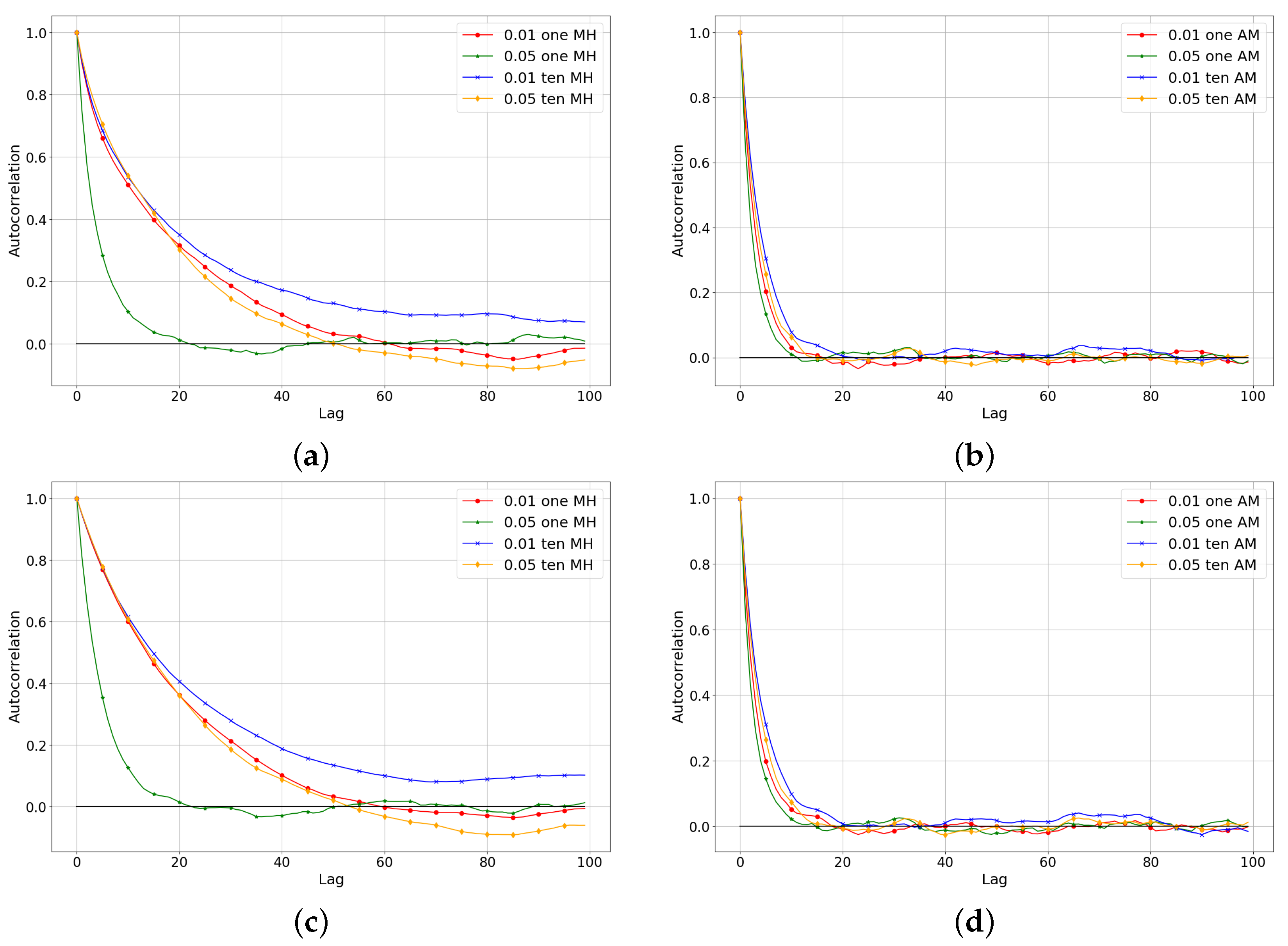
, Figure 5 and Figure 6 uses the following rule to describe: “${\sigma }^2$ N Alg”, where ${\sigma }^2$ stands for noise variance, N—number of measurements, and then the name of the MCMC algorithm. For example, “0.01 ten MH” means a noise variance of 0.01 for ten observations sampled using the Metropolis–Hastings algorithm.

In order to obtain a more quantitative measure of the quality of a sample, it is necessary to look at the correlation structure. The autocorrelation of a signal is a useful tool to analyze the independency of realizations. Autocorrelation calculating as follows: from the generated sample {$x_1,x_2,...,x_N$} of size N = 15,000, calculate the mean,

$$\overline{x}=\frac{1}{N}\sum _{j=1}^N{x}_j,$$

(31)

and the lagged autocorrelations of the centered components,

$$ACF(x,k)=\frac{1}{{\parallel z\parallel }^2}\sum _{j=1}^{N-k}{z}_{j+k}{z}_j, z_j=(x_j-\overline{x}).$$

(32)

Autocorrelations of all cases for MH and AM are presented in Figure 5a and Figure 5b, respectively. For the AM algorithm, the autocorrelation falls off quickly, which says that the chain is well mixed. It is common for the MH algorithm to have high autocorrelation, since it has the Markov property (each subsequent sample is drawn by using the current sample).

When tuning the MH algorithm, necessary to look at the acceptance ratio. The acceptance rate depends on the problem but typically for 1-D problems, the acceptance rate should be around 0.44 for one parameter and around 0.234 for more than five parameters as mentioned earlier. Look at Figure 6, where the plotted acceptance rate exceeds the iteration for all cases that we consider here. For almost all cases, the acceptance rate lies around 0.4 except for two cases: AM with one measurement with noise variance 0.05 and AM with ten measurements with noise variance 0.01. For the first case, this happened due to the fact that the target functional proportional to the posterior distribution is very large and thus has a large acceptance ratio. This is also the reason that in Figure 5a,c the case with 0.05 noise variance for one measurement has small autocorrelation: the MH algorithm has a proposal with a wide step, so the samples get further from each other and the correlation between them reduces. For the second case, on the contrary, this happened due to the fact that the target functional proportional to the posterior distribution has very small sizes and thus has a small acceptance ratio.

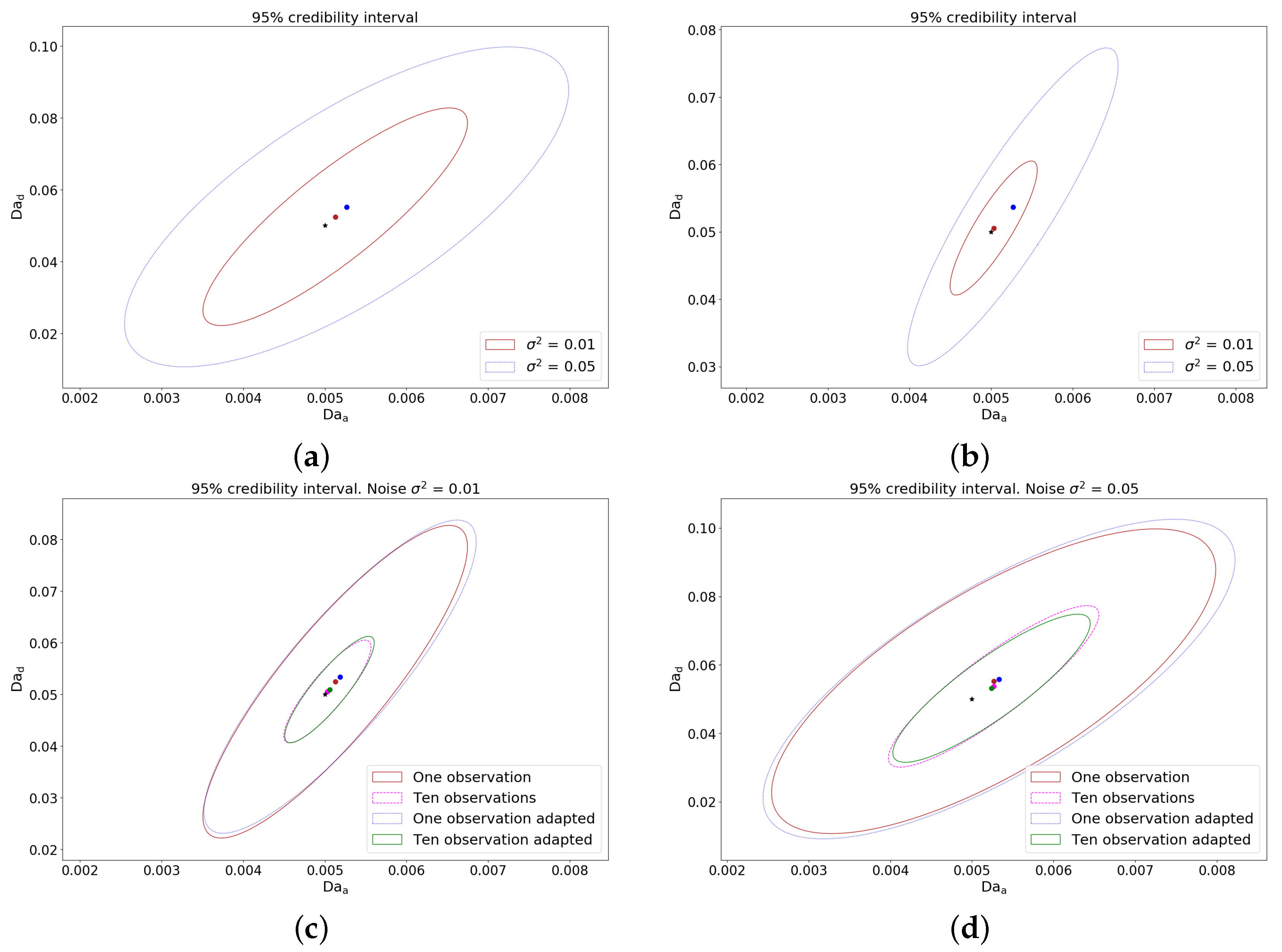
From the posterior PDF, the Bayesian credible interval can be computed, which is the shortest interval containing $95\%$ probability. This means that there is a $95\%$ probability for the observational data, that the true value $\mathbf{\theta }$ falls within credible interval. It is easy to see that in Figure 7c,d MH and AM has just a little differences: AM is slightly smaller. In fact, this is completely normal, as it cannot be better or worse than a well-tuned MH algorithm. In these figures, it can also be seen how credible intervals are reduced with the addition of observations. The obtained results even for noise variance $0.05$ are comparable with work we have done in [22,23] using deterministic and stochastic approaches. The ★ symbol in these figures shows the exact parameters and the • symbol shows the mean values.

It can be seen from the simulation results in Table 1 that the estimated mean and maximum PDF values have a relative error of less than 1%. The last two columns of the table show the error in the $L_2$ norm and have already been converted to percentages.

6. Conclusions

The determination of reaction rates, namely adsorption and desorption parameters for pore scale transport in porous media using MCMC sampling within the framework of Bayesian inference, is discussed. The parameter identification procedure is carried out via the measured concentration of the species at the outlet of the domain. Metropolis–Hastings and Adaptive Metropolis algorithms were implemented and compared. Credible intervals have been plotted from sampled posterior distributions for both algorithms. The impact of the noise in the measurements for the Bayesian estimation procedure is studied. The count of observations was increased up to ten for both algorithms to decrease credible interval. The sample analysis using the autocorrelation function and acceptance rate is performed to estimate mixing of the Markov chain.

The Bayesian approach is a fairly powerful tool, capable not only of identifying the range of acceptable values using a credible interval, not to mention the individual parameters found through the mean or maximum of the posterior density, but also to quantify the associated uncertainty. However, sampling for the Bayesian approach can be quite costly, especially in pore-scale problems, so it may be useful to apply order reduction techniques to the model before applying this approach.

Previously, we conducted research with different approaches on the same mathematical model in the same geometry of the region (for more details, see [23]). The following were implemented: a deterministic approach, where the residual functional was built on a uniform grid; a stochastic approach, when uniformly distributed random points were generated via Sobol sequences [43,44,45] and the functional was constructed from them; the Monte Carlo method, when the functional was built for 10 different realizations of noise, thereby looking at the intersections of the regions of admissible sets. In those approaches, the region of admissible sets was built through a given threshold, which depended on the noise in the observations. Compared to those approaches, all the results obtained in this work are comparable with the previous results. In the Bayesian approach, the region of admissible sets can be determined through the credible interval, where in Figure 7 you can estimate how its size changes depending on the variance of the noise and the number of observations. Compared to previous approaches, this approach is more elegant, but more computationally expensive. The AM algorithm is preferred as it does not need time-consuming tuning like the MH algorithm.

As this article is part of our systematic study and takes into account the results obtained, it is necessary to work on the reduced order model, which we will do in future work.