An Adaptive Covariance Scaling Estimation of Distribution Algorithm

Abstract

Optimization problems are ubiquitous in every field, and they are becoming more and more complex, which greatly challenges the effectiveness of existing optimization methods. To solve the increasingly complicated optimization problems with high effectiveness, this paper proposes an adaptive covariance scaling estimation of distribution algorithm (ACSEDA) based on the Gaussian distribution model. Unlike traditional EDAs, which estimate the covariance and the mean vector, based on the same selected promising individuals, ACSEDA calculates the covariance according to an enlarged number of promising individuals (compared with those for the mean vector). To alleviate the sensitivity of the parameters in promising individual selections, this paper further devises an adaptive promising individual selection strategy for the estimation of the mean vector and an adaptive covariance scaling strategy for the covariance estimation. These two adaptive strategies dynamically adjust the associated numbers of promising individuals as the evolution continues. In addition, we further devise a cross-generation individual selection strategy for the parent population, used to estimate the probability distribution by combing the sampled offspring in the last generation and the one in the current generation. With the above mechanisms, ACSEDA is expected to compromise intensification and diversification of the search process to explore and exploit the solution space and thus could achieve promising performance. To verify the effectiveness of ACSEDA, extensive experiments are conducted on 30 widely used benchmark optimization problems with different dimension sizes. Experimental results demonstrate that the proposed ACSEDA presents significant superiority to several state-of-the-art EDA variants, and it preserves good scalability in solving optimization problems.

1. Introduction

Optimization problems are ubiquitous in daily life and industrial engineering [1,2], such as protein structure prediction [3], community detection [4], control of pollutant spreading [5] and multi-compartment electric vehicle routing [6]. These optimization problems often preserve characteristics such as non-convex, discontinuous, and non-differentiable [7,8,9,10], which greatly challenge the effectiveness of traditional gradient-based optimization algorithms or even make them infeasible [11]. In particular, in the era of big data and the Internet of Things, optimization problems are becoming more and more complex due to the increase in dimensionality [12,13,14]. For instance, some unimodal problems become multimodal with many local optima [15], while some multimodal problems become more complicated with an increasing number of wide and flat local areas [16,17,18]. Such complicated optimization problems are becoming more and more common nowadays, and thus, it is urgent to develop effective optimization algorithms to solve them, so as to promote the development of related fields.

As a kind of gradient-free meta-heuristic algorithm, estimation of distribution algorithm (EDA) mainly maintains a population of individuals to iteratively search the solution space, with each individual representing a feasible solution [19]. During each generation, it selects a number of promising individuals to estimate the probability distribution of the population, and it then randomly samples a new population of solutions based on the estimated probability distribution [20,21]. Due to the randomness in sampling the offspring, EDA preserves high diversity and strong global search ability [22]. Therefore, a lot of researchers have paid extensive attention to developing effective EDAs, and, consequently, not only have EDAs been applied to solve various optimization problems, such as multimodal optimization problems [23] and multi-objective optimization problems [24], but also they have been employed to solve many real-world problems, such as multi-policy insurance investment planning [25] and multi-source heterogeneous user-generated content-driven interactive [22].

In the literature, most EDAs utilize the Gaussian distribution model to evaluate the probability distribution of the population, which is then adopted to sample new solutions [26,27]. During the estimation of the distribution, based on whether the correlation between variables is considered, the current Gaussian estimations of distribution algorithms (GEDAs) are mainly divided into two categories [20,27,28], namely univariate GEDAs (UGEDAs) [29,30,31] and multivariate GEDAs (MGEDAs) [32,33,34,35,36].

UGEDAs [30] consider that each variable is independent on each other. Therefore, the probability distribution of each variable is estimated individually. The most advantageous property of UGEDAs is that the computational cost of the distribution estimation and the offspring sampling is low [31]. However, their effectiveness deteriorates drastically when confronted with optimization problems with interacted variables [29].

Different from UGEDAs, MGEDAs take the correlation among variables into consideration [34], which is realized by estimating the covariance among all variables. With the covariance matrix, MGEDAs could capture the structure of the optimization problem and thus implicitly offer useful information to direct the search of the population [35]. Due to this advantage, MGEDAs achieve much better performance than UGEDAs, especially on problems with many interactive variables [20]. As a result, MGEDAs have been extensively researched in the literature [37,38,39]. However, such superiority of MGEDAs is at the sacrifice of efficiency, as calculating the covariance among all variables is very time-consuming [32].

In MGEDAs, the parameters (i.e., the mean vector and the covariance matrix) of the probability distribution are usually estimated based on a certain number of promising individuals [28]. Specifically, in the probability distribution, the mean vector plays a key role in controlling the center of the offspring to be sampled, while the covariance takes charge of the range of the offspring around the center. In other words, the mean vector makes a crucial influence on the convergence of the population to the optimal areas, while the covariance affects the population diversity [40]. Therefore, to maintain high search diversity for EDAs, many researchers have designed variance or covariance scaling methods [37,41,42,43] to enlarge the sampling range of the estimated probability distribution. However, on the one side, the basic covariance (variance) is still estimated on the same promising individuals selected for the estimation of the mean vector in most existing GEDAs. Therefore, after the covariance (variance) scaling, implemented by multiplying a scaling factor on the estimated covariance (variance) in most covariance scaling methods, the learned structure of the optimization problem, by them, remains unchanged; on the other side, most existing covariance (variance) scaling methods enlarge the estimated covariance (variance) the same degree in different directions.

To remedy the above shortcomings, this paper devises an adaptive covariance scaling method for MGEDAs, leading to an adaptive covariance scaling estimation of distribution algorithm (ACSEDA). Specifically, for the estimation of the mean vector in the probability distribution, it is the same as existing MGEDAs, namely estimating it based on a certain number of promising individuals. However, for the estimation of the covariance in the probability distribution, different from existing MGEDAs, ACSEDA first adaptively enlarges the number of promising individuals, and then, it calculates the covariance on the basis of the scaled promising individuals. In this way, the sampling range of the estimated probability distribution could be enlarged, which is helpful for sampling diversified offspring. As a result, the search diversity of EDA could be amplified, and thus, the chance of falling into local areas could be declined.

As a whole, the main contributions of this paper are summarized as follows:

(1)

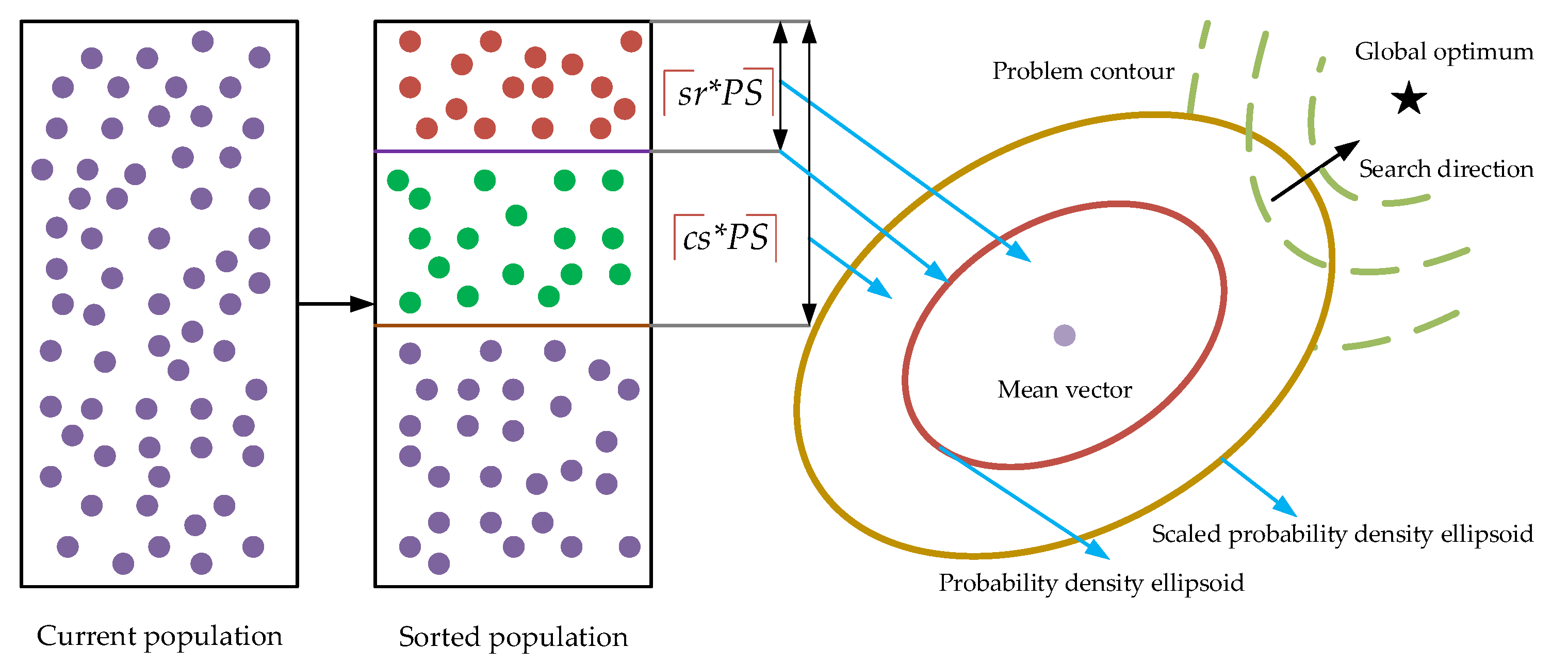
An adaptive covariance scaling method is proposed to adaptively enlarge the sampling range of the estimated probability distribution. Different from most existing covariance scaling methods, we scale the covariance by calculating the covariance based on an amplified number of promising individuals. As a result, not only could the learned structure of the optimization problem captured by the algorithm be improved but the covariance in different directions is also scaled differently. In this way, it is expected that the sampled offspring are not only of high quality, but they are also diversified in different areas.

(2)

An adaptive selection of promising individuals for the estimation of the mean vector is further designed by adaptively decreasing the selection ratio, which is the number of the selected promising individuals out of the whole population. In this way, the estimated mean vector, namely the center of the offspring to be sampled, is gradually close to the promising areas that the current population covers. Therefore, the search process is gradually biased toward exploiting the solution space to refine the solution accuracy. However, it should be mentioned that such a bias is not greedy and not at the serious sacrifice of the population diversity because of the aforementioned covariance scaling technique.

(3)

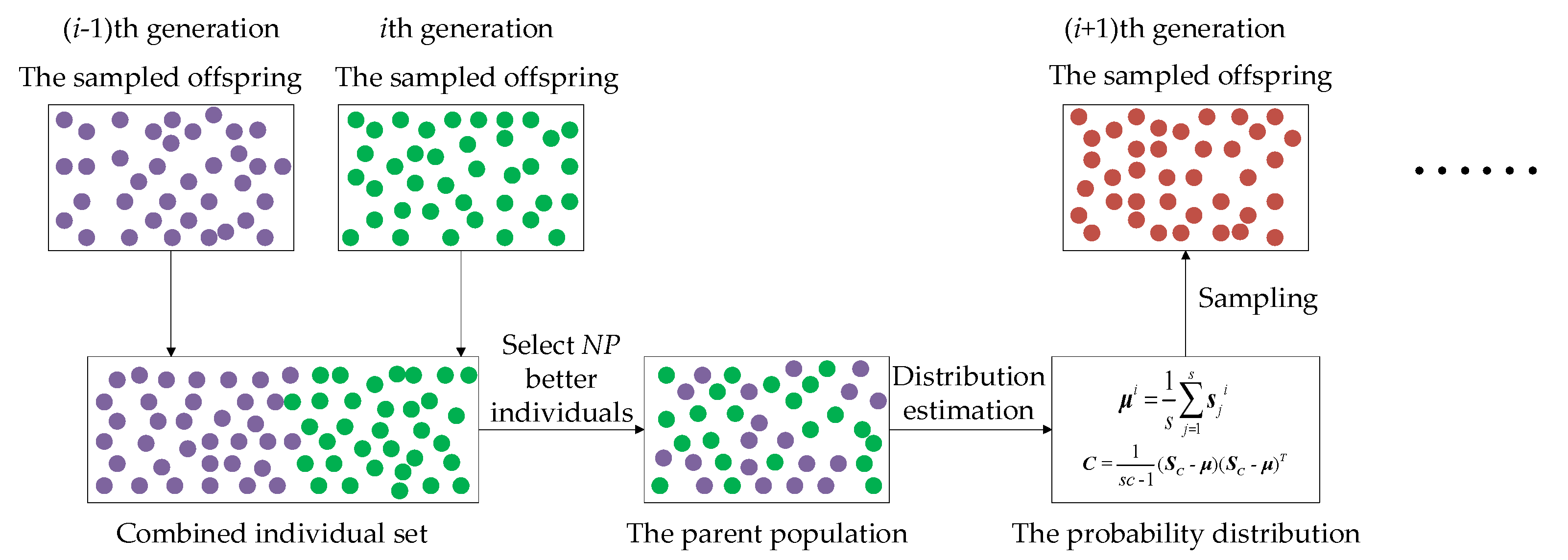
A cross-generation individual selection scheme, for the parent population to estimate the probability distribution, is devised by combining the sampled offspring in the last generation and the one in the current generation to select parent individuals for the next generation. Instead of directly utilizing the sampled offspring as the parent population for the next generation in most existing MGEDAs, the proposed ACSEDA combines the sampled offspring in the last generation and the one in the current generation to select the top half best individuals to form the parent population for the next generation. In this way, the parent population formed is neither too crowded nor too scattered, and thus, the estimated probability distribution is of high quality to sample slightly diversified offspring to approach the optimal areas.

(4)

With the above mechanisms, the proposed ACSEDA is expected to compromise intensification and diversification of the search process well to explore and exploit the solution space and could thus achieve promising performance.

To verify the effectiveness of the proposed ACSEDA, this paper conducts extensive experiments on the widely used CEC2014 [44] benchmark optimization problems, with different dimension sizes, by comparing ACSEDA to 7 state-of-the-art GEDAs. In addition, deep investigations on the components of ACSEDA are also taken to observe what contributes to its promising performance in solving optimization problems.

The remainder of this study is organized as follows: Section 2 reviews related works on GEDAs; then, the proposed ACSEDA is elucidated in detail in Section 3; in Section 4, extensive experiments are conducted to verify the effectiveness of the developed ACSEDA; last, in Section 5, conclusions are presented.

2. Related Work

2.1. Basic GEDA

The overall framework of a general GEDA is outlined in Algorithm 1. As a whole, the basic principle of GEDA is to iteratively build a Gaussian probability distribution model, based on a certain number of promising individuals selected from the current population, and then sample new individuals based on the built probability model for the next generation [21].

Algorithm1: The Procedure of GEDA

Input: population size PS, selection ratio sr; 1: Set g = 0, and randomly initialize the population Pg; 2: Obtain the global best solution Gbest; 3: Repeat 4:   Select $\lceil sr\ast PS\rceil$ promising solutions Sg from Pg; 5:   Build a Gaussian probability distribution model Gg based on Sg; 6:   Randomly generate a new population Pg+1 by sampling from Gg; 7:   Update the global best solution Gbest; 8:   g = g + 1; 9: Until the stopping criterion is met. Output: the global best solution Gbest;

Specifically, as shown in Algorithm 1, given that the population size is PS and the selection ratio is sr (which is the number of selected promising individuals out of the whole population), the number of selected promising individuals in each generation is s = $\lceil sr\ast PS\rceil$. After PS individuals are initialized randomly and evaluated accordingly, as shown in Line 1, the global best solution found so far is obtained (as shown in Line 2). Subsequently, it comes to the main iteration of the algorithm. First, a set (S) of s promising individuals are selected from the current population (Line 4). Then, a Gaussian probability distribution model is estimated based on the selected individuals (Line 5). After that, PS new individuals are randomly sampled based on the estimated Gaussian distribution to form a new population (Line 6). Subsequently, the newly generated individuals are evaluated, and the global best solution is updated. The above process proceeds repeatedly until the termination condition is met. At last, the found global best solution is output.

In GEDAs, the key component is the way to estimate the probability distribution. Different manners of probability distribution estimation result in different kinds of GEDAs. In the literature, based on whether the linkage between variables is considered, existing GEDAs are mainly classified into two categories [20,27,28], namely univariate GEDAs (UGEDAs) [29,30,31,45,46] and multivariate GEDAs [27,32,33,34,35,36].

(1)

UGEDAs: In UGEDAs [29,45,46], each variable is considered to be separable and independent on each other. As a result, the probability distribution of D variables can be estimated separately, and the joint probability distribution of D variables is computed as follows:

$$P(x^1,x^2,\dots ,x^D)={\displaystyle \prod _{i=1}^{D}P(x^i)}.$$

(1)

where P(xⁱ) is the probability distribution of the ith variable, which is estimated as:

$$P(x^i)=\frac{1}{{\sigma }^i\sqrt{2\pi }}{e}^{-\frac{{(x^i-{\mu }^i)}^2}{2{\sigma }^i}}$$

(2)

where uⁱ and σⁱ are the mean value and the variance of the ith variable respectively, which are calculated as follows:

$${\mu }^i=\frac{1}{s}{\displaystyle \sum _{j=1}^s{S}_j{}^i}$$

(3)

$${\sigma }^i=\sqrt{(\frac{1}{s-1}{\displaystyle \sum _{j=1}^s{(S_j{}^i-{\mu }^i)}^2})}$$

(4)

where S is the set of the selected promising individuals, S_jⁱ is the ith dimension of the jth promising individual in S, and D denotes the dimension size of the optimization problem. Based on the estimated probability distribution of each variable, a new solution can be constructed by randomly sampling a new value of each variable separately, based on the associated probability distribution.

(2)

MGEDAs: In MGEDAs [33,34,35,36], the correlations between variables are taken into consideration to estimate the probability distribution. Consequently, different from UGEDAs, the probability distribution of D variables in MGEDAs is estimated together, and the joint probability distribution of D variables is computed as follows:

$$P(x^1,x^2,\dots ,x^D)=\frac{1}{\sqrt{{(2\pi )}^D\left|\mathit{C}\right|}}{e}^{(-\frac{1}{2}{(\mathit{X}-\mathit{\mu })}^T{\mathit{C}}^{-1}(\mathit{X}-\mathit{\mu }))}$$

(5)

where u is the mean vector of the multivariate Gaussian distribution, which is calculated by Equation (3). C is the covariance matrix, which is calculated as follows:

$$\mathit{C}=\frac{1}{s-1}(\mathit{S}-\mathit{\mu }){(\mathit{S}-\mathit{\mu })}^T$$

(6)

Based on the estimated joint probability distribution, a new solution is constructed by jointly sampling values for all variables, randomly, from the multivariate Gaussian distribution model. In general, to make the sampling of new solutions simple, a modified version presented below is usually utilized to generate the offspring in most MGEDAs [32,35]:

$$\begin{array}{l}\mathit{X}=\mathit{\mu }+\mathit{A}\mathit{\Lambda }\mathit{Z}\\ \mathit{Z}\sim N(0,1)\end{array}$$

(7)

$$\mathit{C}=\mathit{A}{\mathit{\Lambda }}^2{\mathit{A}}^T$$

(8)

where A is the eigenvector matrix of C, and Λ is the diagonal matrix whose entries are the square root of the eigenvalues of C. Z is a real number vector, each value of which is randomly sampled from a standard normal distribution separately.

With respect to the computational cost, UGEDAs are less time-consuming, while MGEDAs take more computational cost due to the calculation of the covariance matrix [33,34,35]. However, in terms of the optimization performance, MGEDAs show much better performance, especially on problems with many interacted variables, while UGEDAs only present promising performance on separable optimization problems [29,30,47]. This is because MGEDAs could capture the interaction between variables and thus evolve the population more effectively than UGEDAs [27,37,48].

2.2. Recent Advance of GEDAs

During the optimization, one crucial challenge that most existing GEDAs encounter is the rapid shrinkage of the variance (or the covariance) [20,42,43], which leads to the quickly narrowed sampling range of the probability distribution. This may lead to a quick loss of the search diversity and thus may result in premature convergence and falling into local areas. To remedy this shortcoming, researchers have devoted plenty of attention to designing novel mechanisms to improve the quality of the probability distribution in GEDAs [38,49,50,51].

In [51], the authors demonstrated empirically that high diversity maintenance is very crucial for EDAs to achieve satisfactory performance. Then, based on the findings, they further developed a novel three-step method by combining clustering methods with EDAs to search for the optimal areas with high diversity. To prevent premature convergence in EDAs, Pošík [52] directly multiplied a constant factor on the estimated variance of the Gaussian distribution in each generation to enlarge the sampling range. In [43], Grahl et al. proposed a correlation-triggered adaptive variance scaling strategy to reduce the risk of premature convergence and then embedded it into the iterated density–estimation evolutionary algorithm (IDEA). Specifically, similar to [52], the proposed method multiplies a factor to the estimated variance. The difference lies in such a factor not being constant but dynamically adjusted during the evolution, based on whether the global best solution is improved or not. In addition, such adjustment is triggered based on the correlation between the ranks of the normal density and the fitness of the selected solutions. To further trigger the dynamic adjustment of the scaling factor properly, in [42], Bosman et al. proposed a novel indicator, named Standard–Deviation Ratio (SDR), to trigger the adjustment adaptively. Specifically, based on this indicator, the variance scaling is triggered only when the improvements are found to be far away from the mean vector. In [53], a cross-entropy based adaptive variance scaling method was proposed. In this method, the difference between the sampled population and the prediction of the probabilistic model is first measured, and the scaling factor on the variance is then computed by minimizing the cross-entropy between the two distributions.

Different from the above variance scaling methods that directly multiply a scaling factor on the estimated variance, in [49], the authors proposed a novel probability density estimator based on the new mean vector obtained by the anticipated mean shift strategy. Then, once the new mean vector gets better, the variance estimator adaptively enlarges the variance without using an explicit factor, but rather, by using the new better mean vector to calculate the variance. Furthermore, they also developed a reflecting sampling strategy to further improve the search efficiency of GEDA. Accompanied with these two schemes, a new GEDA variant named EDA_VERS [49] was developed. Subsequently, a novel anisotropic adaptive variance scaling (AAVS) method was proposed in [41], and a new GEDA named AAVS-EDA was designed. Specifically, in this algorithm, a topology-based detection method was devised to detect the landscape characteristics of the optimization problems, and then, based on the captured characteristics, the variances along different eigen-directions are anisotropically scaled. In this way, the variances and the main search direction of GEDA could be simultaneously adjusted. Recently, Liang et al. proposed a new GEDA variant, named EDA2 [37], to improve the optimization performance of EDA. Specifically, instead of only utilizing promising individuals in the current generation to estimate the Gaussian model, this algorithm stores historical high-quality individuals generated in the previous generations into an archive and adopts these individuals to collaboratively estimate the covariance of the Gaussian model. In this manner, valuable historical evolution information could be integrated into the estimated model.

The above mentioned MGEDAs usually adopt the full rank covariance matrix to estimate the covariance. Since the calculation of the full-rank covariance matrix is very time-consuming, the computational complexity of most MGEDAs is usually high. To alleviate this shortcoming, researchers turn to seeking efficient covariance matrix adaption (CMA) techniques for EDA [54]. As for the covariance matrix, a direct and simple method to speed up its computation is to reduce the degrees of freedom. To this end, Ros and Hansen [55] proposed to only update the elements in the diagonal of the covariance matrix, leading to a de-randomized evolution strategy, named sep-CMA-ES. This method reduces the updating time and space complexity of the covariance matrix from quadratic to linear. In [56], the authors devised an adaptive diagonal decoding scheme to accelerate covariance matrix adaptation. Further, ref. [57] developed a matrix-free CMA strategy by employing combinations of difference vectors between archived individuals and random vectors, generated by the univariate Gaussian distribution along directions of the past shifts of the mean vector. In [58], Beyer and Sendhoff proposed a matrix adaptation evolution strategy (MA-ES) by removing one evolution path in the calculation of the covariance matrix, leading to that the covariance update is no longer needed. In [59], Li and Zhang first designed a rank one evolution strategy by using a single principal search direction, which is of linear complexity. Then, they developed a rank-m evolution strategy by employing multiple search directions. In particular, these two evolution strategies mainly adopt principal search directions to seek for the optimal low rank approximation to the covariance matrix. In [60], He et al. put forward a search direction adaptation evolution strategy (SDA-ES) with linear time and space complexity. Specifically, this algorithm first models the covariance matrix with an identity matrix along with multiple search directions. Then, it uses a heuristic to update the search directions such as the principal component analysis.

Besides the advance of GEDAs in covariance (or variance) scaling and adaption, some researchers have also attempted to design new ways to shift the mean vector of the Gaussian distribution model. For instance, in [61], Bosman et al. proposed an anticipated mean shift to update the mean vector and then used the updated mean vector to calculate the variance. In addition, some researchers have also attempted to adopt other distribution models, instead of the Gaussian distribution model, to estimate the probability distribution. For example, in [62], a probabilistic graphical model was designed to consider the dependencies between multivariate variables. Specifically, in this algorithm, a parallel of a certain number of subgraphs, with a smaller number of variables, is estimated separately to capture the dependencies among variables in each subgraph. Then, each estimated graph model associated with the subgraph samples new values for the associated variables separately. In [39], the authors utilized the Boltzmann distribution to build the probability distribution model in EDA, leading to BUMDA. In particular, the distribution parameters are derived from the analytical minimization of the Kullback–Leibler divergence. In [50], the authors devised a novel multiple sub-models maintenance technique for EDA, leading to a new EDA variant, named maintaining and processing sub-models (MAPS). Specifically, this algorithm maintains multiple sub-models to detect promising areas.

Since EDAs utilize the estimated probability distribution model to sample new solutions, they generally lack subtle refinement to improve the solution accuracy [63]. To fill this gap, local search methods are commonly accompanied with EDAs to refine the found promising solutions [38,49,50]. For instance, in [64], simulated annealing (SA) based local search operator was incorporated into EDA to balance the exploration and exploitation to search the solution space properly. Specifically, the SA-based local search is probabilistically executed on some good solutions to improve their accuracy. To improve the solution accuracy, Zhou et al. [38] developed cheap and expensive local search methods for EDA, leading to a new EDA variant named EDA/LS. In particular, this EDA variant adopts a modified univariate histogram probabilistic model to sample a part of individuals, and it then utilizes a cheap local search method to sample the rest of the individuals. Besides, it also employs an expensive local search method to refine the found promising solutions. Along this direction, an extension of EDA/LS, named EDA/LS-MS, was developed in [65] by introducing a mean shift strategy to replace the cheap local search method in EDA/LS to refine some good parent solutions.

Though a lot of remarkable GEDA variants have emerged and shown promising performance in solving optimization problems, they still encounter limitations, such as falling into local areas and premature convergence. In particular, it is found that most existing GEDAs estimate the variance (or covariance) based on the same selected promising individuals used for the estimation of the mean vector. Although various variance (or covariance) scaling methods [37,43,49,53,66] and covariance matrix adaption methods [56,57,58,59,60] have been proposed to improve the sampling range of the estimated probability distribution model, on the one hand, the structure of the optimization problem captured by most existing GEDA variants remains unchanged after the scaling; on the other hand, most existing variance (covariance) scaling methods scale the estimated variance (covariance) equally in different directions. This is actually not beneficial to effectively sample new promising individuals.

To alleviate the above concern, this paper devises an adaptive covariance scaling EDA by adaptively enlarging the number of promising individuals (as compared with those for the mean vector estimation) to estimate the covariance. In this way, not only does the structure of the optimization problem captured by the algorithm become better, but also the covariance is scaled differently in different directions.

3. Proposed ACSEDA

To improve the effectiveness of EDA in solving optimization problems, this paper proposes an adaptive covariance scaling EDA (ACSEDA) by introducing more promising individuals to calculate the covariance. Furthermore, to alleviate the sensitivity of the proposed ACSEDA to parameters, this paper further devises two adaptive strategies for the two key parameters in ACSEDA. The components of ACSEDA are elucidated as follows.

3.1. Adaptive Covariance Scaling

In traditional GEDAs [27], both the mean vector and the covariance of the multivariate Gaussian distribution model are estimated based on the selected promising individuals. Then, on the basis of the estimated probability distribution model, the offspring are sampled randomly. In particular, we can see that the mean vector has a great influence on the convergence speed of GEDAs to promising areas, while the covariance mainly takes charge of the sampling range of the distribution model, which plays a significant role in high diversity maintenance.

During the evolution, the population gradually approaches the promising areas and the selected promising individuals used for probability distribution estimation are gradually aggregated together as well. In this situation, the estimated covariance would become smaller and smaller. Once the estimated mean vector falls into local areas, the sampled offspring could hardly escape from local areas. As a consequence, the population falls into local areas, and premature convergence occurs. Such a predicament is encountered by many existing GEDAs [20].

To alleviate this issue, this paper proposes a covariance scaling strategy to enlarge the covariance by introducing more promising individuals on the basis of the selected individuals for the estimation of the mean vector. Specifically, given the population size is PS, s = $\lceil sr\ast PS\rceil$ promising individuals are first selected from the population to estimate the mean vector of the probability distribution, where sr is the selection ratio, defined as the number of selected individuals out of the population. Then, different from most existing GEDAs [67], which estimate the covariance based on the sc = $\lceil cs\ast PS\rceil$ individuals as well, this paper selects sc promising individuals to estimate the covariance, where cs is the covariance scaling parameter, which is the number of the promising individuals out of the population and is usually larger than sr. In this way, more promising individuals are selected to participate in the estimation of the covariance and thus, the covariance is enlarged.

As shown in Figure 1, after the population is sorted from the best to the worst with respect to the fitness, s best individuals are selected to form the promising individual set S, and then, the mean vector u is estimated based on S according to Equation (3). Subsequently, different from most existing GEDAs, the proposed covariance scaling method selects sc best individuals to form the promising individual set S_C to estimate the covariance. It should be mentioned that cs is usually larger than sr, which also indicates that S_C is larger than S. In this way, S is a subset of S_C. Subsequently, instead of using S to calculate the covariance according to Equation (6), the proposed method utilizes S_C, namely an enlarged individual set, to estimate the covariance as follows:

$$\mathit{C}=\frac{1}{sc-1}({\mathit{S}}_{\mathit{C}}-\mathit{\mu }){({\mathit{S}}_{\mathit{C}}-\mathit{\mu })}^T$$

(9)

As shown in Figure 1, since more promising individuals participate in the estimation of the covariance, the sampling range of the estimated probability distribution model is enlarged. On the one hand, the sampled offspring based on this model are more diversified, which is very beneficial for the population to avoid falling into local areas. On the other hand, it might also be likely to generate more promising individuals close to the promising areas, and thus, the convergence could also be strengthened to some extent.

Remark 1.

It deserves attention that different from existing covariance scaling methods, which scales the covariance directly with a fixed scalar, the proposed covariance scaling method estimates the covariance based on an enlarged number of promising individuals as compared to those for the estimation of the mean vector. This brings the following two benefits for the estimated probability distribution model:

(1) 

By introducing more promising individuals, the proposed scaling method enlarges the covariance differently in different directions between variables and thus it implicitly takes the difference between variables into consideration. However, existing scaling methods [37] enlarge the covariance with a same scalar and hence they do not consider the difference between variables.

(2) 

The proposed scaling method is likely to better capture the structure of the optimization problem with respect to the correlations between variables by introducing more promising individuals. Nevertheless, the structure captured by existing scaling methods remains unchanged after the scaling.

Taking a deep investigation on the parameter cs, in the proposed covariance scaling method, we find that neither a too large cs, nor a too small cs are proper to aid EDA to achieve promising performance. On the one side, a too-large cs may lead to a too large sampling range of the probability distribution. This may result in too diversified offspring sampled from the distribution model. In particular, it is found that, in the early stage of the evolution, a large cs may be beneficial to maintain a large sampling range and thus sample diversified offspring. This is helpful for EDA to explore the solution space in very different directions, whereas, in the late stage, such a setting of cs is not appropriate because it is not beneficial for the population to extensively exploit the found promising areas to refine the solution accuracy. On the other side, a too-small cs may bring in a too-small sampling range of the distribution model, which may sample concentrated offspring. Though it is desirable in the late stage of the evolution, it is not suitable during the whole evolution, because it may increase the risk of EDA in falling into local areas. Consequently, based on the above analysis, it is found that cs should not be fixed, but dynamically adjusted during the evolution process.

To the above end, this paper further designs an adaptive strategy for cs as follows:

$$cs=1-(1-s{r}_{\min }){(\frac{FEs}{FE{s}_{\max }})}^2$$

(10)

where sr_min denotes the lower bound of the selection ratio sr used for the estimation of the mean vector of the multivariate Gaussian distribution model, FEs_max is the maximum number of fitness evaluations, while FEs denotes the used number of fitness evaluations up to the current generation.

From Equation (10), we can see that cs decreases from 1.0 to sr_min as the evolution continues. Specifically, it is found that, in the early stage, most individuals in the population are used to estimate the covariance. This brings two benefits for EDA: (1) the sampling range of the probability distribution model is large and thus the sampled offspring are diversified and scatter dispersedly to explore the solution space. It is not only beneficial for the population to find more promising areas, but it is also very profitable for the population to avoid falling into local areas. (2) The captured structure of the optimization problem tends to be global and accurate with a large number of promising individuals. In the early stage, the individuals are usually scattered diversely in the solution space. In this situation, the captured structure of the optimization problem is usually global. Therefore, to accurately capture the correlations between variables globally, a large number of promising individuals are usually needed. Consequently, in the early stage, it is helpful to capture an accurate structure of the optimization problem when cs is large.

Conversely, in the late stage, from Equation (10), it is found that cs becomes smaller and smaller. This leads to a narrow sampling range of the probability distribution. Therefore, the sampled offspring are concentrated and surrounded around the mean vector. In this situation, the population exploits the found promising areas, and thus, the accuracy of the solution can be improved.

To summarize, with the above adaptive covariance scaling scheme, the proposed EDA variant is expected to obtain a promising balance between diversification and intensification of the population. Therefore, the algorithm could explore and exploit the complicated solution space properly to obtain promising performance in solving complicated optimization problems.

3.2. Adaptive Promising Individuals Selection

In GEDAs, the number (s = $\lceil sr\ast PS\rceil$) of selected promising individuals, for the estimation of the mean vector, makes a significant influence on the convergence speed of EDAs. As shown in Figure 1, the mean vector mainly takes control of the center of the sampled offspring. A too-large sr may lead to that a large number of promising individuals being used to estimate the mean vector. As a result, the estimated mean vector may be too far away from the promising areas. In the early stage of the evolution, this is beneficial for EDAs to maintain high search diversity. Nevertheless, in the late stage of the evolution, a large sr may slow down the convergence of the population to find high-quality solutions. On the contrary, a too-small sr may result in the estimated mean vector being too close to the promising areas. This case is suitable, in the late stage of the evolution, to exploit the found promising areas. However, it may lead to premature convergence if we keep sr small during the whole evolution, especially when the selected promising individuals all fall into local areas.

Based on the above analysis, it might as well dynamically adjust sr during the evolution. To this end, this paper devises a simple adaptive strategy for sr as follows:

$$sr=s{r}_{\max }-(s{r}_{\max }-s{r}_{\min })(\frac{FEs}{FE{s}_{\max }}{)}^{0.1}$$

(11)

where sr_max and sr_min represent the maximum selection ratio and the minimum selection ratio, which accordingly determine the maximum number (s_max = $\lceil {sr}_{\max }\ast PS\rceil$) and the minimum number (s_min = $\lceil {sr}_{\min }\ast PS\rceil$) of the selected promising individuals. In this paper, we set them as 0.35 and 0.05, respectively.

From Equation (11), we can see that in the early stage, sr is large, and then, it decreases gradually as the evolution goes. This indicates that during the evolution, the mean vector of the estimated probability distribution is becoming closer and closer to the promising areas. In this way, the population gradually tends to exploit the found promising areas.

Remark 2.

In particular, compared Equation (11) with Equation (10), as shown in Figure 2, the following findings can be obtained:

(1) 

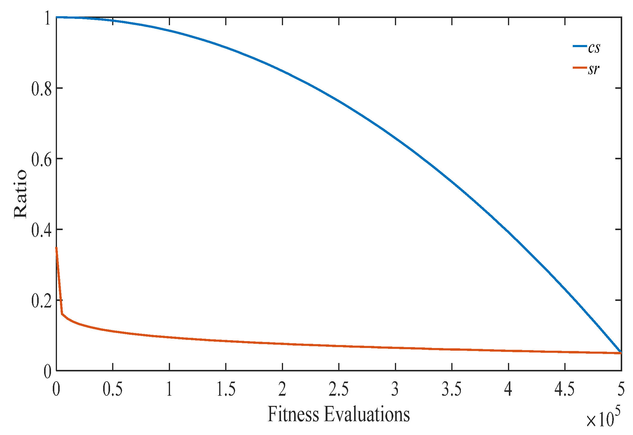
srdecreases dramatically in the early stage, and mildly in the late stage, while cs decreases mildly in the early stage, and dramatically in the late stage. This actually matches the expectation that the proposed ACSEDA should explore the solution space in the early stage without serious loss of convergence, while it should exploit the search space in the late stage without serious sacrifice of search diversity. For one thing, in the early stage, sr decreases rapidly and thus the estimated mean vector is close to the promising areas that the current population lies. However, it should be mentioned that in such a situation, the sampling diversity of the estimated probability distribution is not declined, because the estimated covariance is large due to the large cs. On the contrary, in this situation, the sampling quality of the estimated probability distribution could be improved due to the high-quality mean vector and thus the population could effectively explore the search space to find promising areas in the early stage. In the late stage, sr decreases mildly, while cs descends quickly. In this situation, the quality of the mean vector is gradually promoted by approaching the promising areas closer and closer. At the same time, the sampling range of the estimated distribution gradually shrinks due to the covariance estimated on the reduced number of promising individuals. Therefore, in the late stage, ACSEDA gradually biases to exploiting the found promising areas to improve the solution quality. However, it should be mentioned that such a bias is not at the serious sacrifice of the search diversity because of the proposed covariance scaling technique.

(2) 

csis always larger than sr during the evolution and the gap between cs and sr gradually shrinks as the evolution goes. This indicates that during the evolution, compared with traditional GEDAs, the covariance is always amplified, so that the estimated probability distribution could sample diversified offspring around the estimated mean vector with high quality. In addition, the gradually narrowed difference between sr and cs indicates that the scaling of the covariance is gradually declined. This implies that the proposed ACSEDA gradually concentrates on exploiting the solution space to refine the solution accuracy.

3.3. Cross-Generation Individual Selection for Parent Population

In traditional EDAs [28], the offspring is directly utilized as the parent population for the next generation to estimate the probability distribution model. Since the quality of the sampled offspring is uncertain, the quality of the estimated probability distribution model may not be improved or even degrade compared with the estimated probability distribution in the last generation. This may slow down the convergence of the population to promising areas. Therefore, to remedy this shortcoming, some EDA variants [68] combine the offspring and the parent population together and then select the best PS individuals as the parent population for the next generation. However, such selection is too greedy and thus may lead to premature convergence and falling into local areas.

To alleviate the above predicament, and to further make a promising compromise between convergence and diversity, this paper further devises a cross-generation individual selection strategy for the parent population.

As Figure 3 shows, this paper combines the sampled offspring in the last generation and the sampled offspring in the current generation and then selects the best PS individuals as the parent population for the next generation to estimate the probability distribution model. In this way, the historical information in the last generation can be utilized to build the probability distribution model.

Remark 3.

Different from existing individual selection methods [26,48,69], the proposed cross-generation individual selection strategy takes advantage of the sampled offspring in the two consecutive generations to select individuals for the parent population in the next generation. Such a selection strategy brings the following benefits to ACSEDA:

(1) 

Individuals in the parent populationare diversified.The sampled offspring in the last generationusually have big difference with the offspring in the current generation.Combining them together to select individuals is less likely to generate crowded individuals for the parent population. As a result, the estimated probability distribution model is less likely to fall into local areas andat the same time, has a wide sampling range to generate diversified offspring. In this way, ACSEDA could preserve high search diversity during the evolution.

(2) 

With this strategy, the latest historical promising individuals in the last generation could be integrated with those in the current offspring. As a consequence, individuals in the parent population are not only diversified, but also of high quality. Hence, the estimated probability distribution is of high quality to generate more promising offspring. By this means, the convergence of ACSEDA could be guaranteed.

(3) 

With this selection strategy, ACSEDA is further expected to preserve a good compromise between exploration and exploitation to search the solution space effectively.Experiments conducted in Section 4will demonstrate the effectiveness of the proposed cross-generation individual selection strategy.

3.4. Overall Procedure of ACSEDA

Combining the above three schemes together, the proposed ACSEDA is outlined in Algorithm 2. Specifically, after the initialization of the population (Line 2), the algorithm goes to the main iteration loop for evolution (Lines 5–16). In the main loop, it first executes the proposed adaptive promising individual selection strategy for the estimation of the mean vector (Lines 6 and 7). Then, it comes to the proposed adaptive covariance scaling strategy to estimate the covariance of the probability distribution model (Lines 8 and 9). Subsequently, the offspring are randomly sampled based on the estimated probability distribution model (Line 10). Hereafter, it arrives at the proposed cross-generation individual selection strategy to select individuals for the parent population in the next generation (Line 12). At last, a local search method is conducted on the global best solution to refine its accuracy (Line 14).

Algorithm 2: The Procedure of ACSEDA

Input: population size PS; 1: Set FEs = 0; 2: Initialize PS individuals randomly and evaluate their fitness; 3: FEs = FEs + PS; 4: Obtain the global best solution Gbest and store the current population; 5: While (FEs < FEsmax) 6:     Calculate the selection ratio sr according to Equation (11); 7:     Select $\lceil sr\ast PS\rceil$ promising solutions from the population and calculate the mean value μ using Equation (3); 8:     Calculate the covariance scaling parameter cs according to Equation (10); 9:     Estimate the covariance matrix C according to Equation (9); 10:   Randomly sample PS new individuals based on the estimated multivariate Gaussian model, evaluate their fitness and store them; 11:   FEs = FEs + PS; 12:   Combine the offspring in the last generation and the offspring in the current generation to select PS better individuals to form the parent population for the next generation; 13:   Update the global best solution Gbest; 14:   Execute local search 2 times on Gbest; 15:   FEs = FEs +2; 16:   End While Output: the global best solution Gbest;

In Algorithm 2, it should be noticed that a local search strategy is additionally added to improve the solution accuracy of the global best solution. This is because EDAs are probability distribution model based optimization algorithms, and as a consequence, EDAs usually lack strong local exploitation [26,38,70]. Therefore, in the literature [23,38,70], local search methods are generally accompanied by EDAs to improve the solution quality. Hence, the same as most existing EDA variants [23,26,38,70,71], ACSEDA also adopts a local search method to refine the global best solution, as shown in Line 14.

For simplicity and keeping consistent with the probability distribution model in ACSEDA, this paper applies the univariate Gaussian distribution with a small variance to execute the local search on the global best solution. In this paper, the small variance is set as 1.0 × 10⁻⁴. In addition, for saving computational resources, we execute the local search method on the global best solution only two times, as shown in Line 14.

As a whole, with the proposed three main techniques and the local search method, ACSEDA is expected to explore and exploit the solution space properly to locate the optima of optimization problems.

4. Experimental Studies

This section mainly conducts extensive experiments to verify the effectiveness of the proposed ACSEDA. Specifically, the commonly used CEC 2014 benchmark problem set [44] is adopted in this paper. This benchmark set contains 30 various complicated optimization problems, such as unimodal problems, multimodal problems, hybrid problems, and composition problems. For detailed information on this benchmark set, please refer to [44].

4.1. Experimental Settings

First, to comprehensively demonstrate the effectiveness of the proposed ACSEDA, we select several state-of-the-art EDA variants to make comparisons in solving the complicated CEC 2014 benchmark problems. Specifically, the selected state-of-the-art EDA variants are EDA2 [37], EDA_VERS [49], EDA/LS [38], EDA/LS-MS [65], MA-ES [58], and BUMDA [39]. In addition, as a baseline method, the traditional multivariate Gaussian model based EDA [28] is also utilized as a compared method. To tell it apart from the others, we denote it as TRA-EDA in the experiments.

Second, to make comprehensive comparisons between the proposed ACSEDA and the above compared EDA variants, we compare their optimization performance in solving the CEC 2014 problems with three different dimension sizes, namely 30-D, 50-D, and 100-D. For fairness, the maximum number of fitness evaluations (FEs_max) is set as 10,000$\ast$D for all algorithms.

Third, for fair comparisons, the key parameter settings of the compared algorithms are set, as recommended, in the associated papers. For the population size, we tune the settings of all algorithms on the CEC 2014 benchmark set with different dimension sizes. Specifically, after preliminary experiments, the parameter settings of all algorithms are shown in

Table 1. Parameter settings of ACSEDA and the compared algorithms.

Algorithm		ACSEDA	EDA/LS					EDA2		EDA/LS-MS					EDAVERS		BUMDA	TRA-EDA		MA-ES
Parameter		PS	PS	M	Pb	Pc	θ	PS	l	PS	M	Pa	Pb	θ	PS	sr	PS	PS	sr	PS	mu
D	30	1300	150	15	0.2	0.2	0.1	100	20	150	15	0.2	0.2	0.1	500	0.35	900	2500	0.2	$4+\lfloor 3\ast \ln D\rfloor$	$|PS/2|$
	50	1800	150					200		1000					600		1100	4700
	100	3200	150					300		2000					700		1500	6000

.

Fourth, to comprehensively evaluate the optimization performance of each algorithm, we execute each algorithm independently for 30 runs and utilize the median, mean, and standard deviation values over the 30 independent runs to evaluate its optimization performance. Furthermore, to tell the statistical significance, we conduct the Wilcoxon rank-sum test, at the significance level of α = 0.05, to compare the proposed ACSEDA with each associated EDA variant. In addition, to compare the overall optimization performance of all algorithms on the whole CEC 2014 benchmark set, we further conduct the Friedman test at the significance level of α = 0.05 by taking advantage of the mean value of each algorithm on each function in the benchmark set.

At last, it deserves attention that all algorithms are programmed under MATLAB R2018a, and they are run on the same computer with Intel(R) Core(TM) i7-10700T CPU @ 2.90 GHz 2.90 GHz and 8 G RAM.

4.2. Comparison with State-of-the-Art EDAs

Table 2. Comparison between ACSEDA and the compared state-of-the-art EDA variants on the 30-D CEC2014 benchmark problems. The bold results indicate that ACSEDA is significantly better than the compared methods.

F	Category	Quality	ACSEDA	EDA2	EDAVERS	EDA/LS	EDA/LS-MS	TRA-EDA	BUMDA	MA-ES
F1	Unimodal Problems	Median	0.00 × 100	0.00 × 100	6.48 × 104	1.90 × 10−9	1.83 × 10−9	6.94 × 107	1.15 × 108	1.42 × 10−14
		Mean	0.00 × 100	0.00 × 100	7.76 × 104	9.09 × 101	1.98 × 101	6.80 × 107	1.16 × 108	1.37 × 10−14
		Std	0.00 × 100	0.00 × 100	4.85 × 104	4.89 × 102	1.07 × 102	1.17 × 107	2.12 × 107	2.55 × 10−15
		p-value	-	NaN=	1.21 × 10−12+	1.21 × 10−12+	1.21 × 10−12+	1.21 × 10−12+	1.21 × 10−12+	1.17 × 10−13+
F2		Median	0.00 × 100	0.00 × 100	2.54 × 103	1.48 × 10−11	4.59 × 10−11	6.61 × 109	1.80 × 104	2.84 × 10−14
		Mean	0.00 × 100	0.00 × 100	2.36 × 103	2.52 × 10−10	1.45 × 10−10	6.58 × 109	5.15 × 105	2.65 × 10−14
		Std	0.00 × 100	0.00 × 100	8.94 × 102	5.04 × 10−10	2.43 × 10−10	1.05 × 109	2.45 × 106	7.09 × 10−15
		p-value	-	NaN=	1.21 × 10−12+	1.21 × 10−12+	1.21 × 10−12+	1.21 × 10−12+	1.21 × 10−12+	7.15 × 10−13+
F3		Median	0.00 × 100	0.00 × 100	1.41 × 103	8.42 × 10−9	8.85 × 10−10	9.83 × 103	6.49 × 103	5.68 × 10−14
		Mean	0.00 × 100	0.00 × 100	1.44 × 103	3.10 × 10−9	2.34 × 10−9	1.00 × 104	6.52 × 103	5.68 × 10−14
		Std	0.00 × 100	0.00 × 100	5.54 × 102	4.33 × 10−9	4.21 × 10−9	1.97 × 103	1.85 × 103	5.05 × 10−29
		p-value	-	NaN=	1.21 × 10−12+	1.21 × 10−12+	1.21 × 10−12+	1.21 × 10−12+	1.21 × 10−12+	1.69 × 10−14+
F1–3	w/t/l		-	0/3/0	3/0/0	3/0/0	3/0/0	3/0/0	3/0/0	3/0/0
F4	Simple Multimodal Problems	Median	3.25 × 100	0.00 × 100	6.39 × 10−1	1.02 × 10−9	4.75 × 10−9	7.93 × 102	9.74 × 101	5.68 × 10−14
		Mean	3.15 × 100	0.00 × 100	6.14 × 10−1	1.33 × 10−1	2.66 × 10−1	7.72 × 102	9.88 × 101	2.66 × 10−1
		Std	1.02 × 100	0.00 × 100	2.76 × 10−1	7.16 × 10−1	9.94 × 10−1	1.27 × 102	2.69 × 101	9.94 × 10−1
		p-value	-	1.21 × 10−12−	3.82 × 10−10−	2.15 × 10−10−	1.41 × 10−9−	3.02 × 10−11+	3.02 × 10−11+	1.69 × 10−10−
F5		Median	2.09 × 101	2.10 × 101	2.10 × 101	2.00 × 101	2.00 × 101	2.09 × 101	2.10 × 101	2.00 × 101
		Mean	2.09 × 101	2.09 × 101	2.09 × 101	2.00 × 101	2.00 × 101	2.09 × 101	2.10 × 101	2.04 × 101
		Std	4.96 × 10−2	4.86 × 10−2	7.13 × 10−2	5.47 × 10−6	3.43 × 10−2	5.47 × 10−2	5.00 × 10−2	6.93 × 10−1
		p-value	-	7.01 × 10−2=	7.48 × 10−2=	1.17 × 10−11−	9.37 × 10−12−	8.77 × 10−1=	2.32 × 10−2+	3.96 × 10−4−
F6		Median	1.99 × 10−6	0.00 × 100	1.77 × 10−5	4.09 × 101	3.81 × 101	4.58 × 10−1	1.50 × 100	2.25 × 101
		Mean	2.07 × 10−6	2.09 × 10−1	4.76 × 10−1	4.05 × 101	3.84 × 101	5.16 × 10−1	1.61 × 100	2.24 × 101
		Std	8.29 × 10−7	5.63 × 10−1	8.19 × 10−1	2.14 × 100	2.75 × 100	4.43 × 10−1	1.12 × 100	4.08 × 100
		p-value	-	3.82 × 10−5+	6.61 × 10−1=	3.02 × 10−11+	3.02 × 10−11+	3.02 × 10−11+	1.07 × 10−7+	3.02 × 10−11+
F7		Median	0.00 × 100	0.00 × 100	1.14 × 10−13	2.21 × 10−2	3.69 × 10−2	9.12 × 101	3.24 × 10−2	1.14 × 10−13
		Mean	0.00 × 100	0.00 × 100	1.06 × 10−13	3.52 × 10−2	4.84 × 10−2	9.01 × 101	9.35 × 10−2	2.79 × 10−3
		Std	0.00 × 100	0.00 × 100	2.84 × 10−14	4.56 × 10−2	6.23 × 10−2	1.25 × 101	1.41 × 10−1	4.40 × 10−3
		p-value	-	NaN=	7.15 × 10−13+	1.20 × 10−12+	1.19 × 10−12+	1.21 × 10−12+	1.21 × 10−12+	3.85 × 10−13+
F8		Median	9.95 × 10−1	6.47 × 100	1.52 × 102	2.27 × 102	2.06 × 102	1.49 × 101	0.00 × 100	1.68 × 102
		Mean	1.16 × 100	6.60 × 100	1.32 × 102	2.38 × 102	2.13 × 102	1.54 × 101	0.00 × 100	1.68 × 102
		Std	8.93 × 10−1	1.81 × 100	5.09 × 101	6.69 × 101	6.08 × 101	3.39 × 100	0.00 × 100	3.98 × 100
		p-value	-	1.92 × 10−11+	3.86 × 10−11+	2.13 × 10−11+	2.13 × 10−11+	2.13 × 10−11+	4.26 × 10−9−	2.02 × 10−11+
F9		Median	9.95 × 10−1	5.47 × 100	1.48 × 102	3.33 × 102	3.20 × 102	1.10 × 101	9.95 × 10−1	1.87 × 102
		Mean	1.16 × 100	5.80 × 100	1.31 × 102	3.28 × 102	3.18 × 102	1.13 × 101	1.41 × 100	1.88 × 102
		Std	9.29 × 10−1	1.69 × 100	4.96 × 101	6.66 × 101	4.01 × 101	2.68 × 100	1.05 × 100	5.42 × 100
		p-value	-	2.85 × 10−11+	1.13 × 10−11+	2.40 × 10−11+	2.40 × 10−11+	2.40 × 10−11+	2.03 × 10−2+	2.10 × 10−11+
F10		Median	3.59 × 100	6.33 × 100	5.69 × 103	4.76 × 103	4.04 × 103	2.39 × 102	2.84 × 101	3.88 × 103
		Mean	1.13 × 101	5.28 × 101	5.62 × 103	4.76 × 103	4.11 × 103	2.86 × 102	3.81 × 101	3.90 × 103
		Std	2.89 × 101	8.32 × 101	3.90 × 102	1.24 × 103	8.86 × 102	1.98 × 102	5.51 × 101	3.24 × 102
		p-value	-	2.10 × 10−3+	3.02 × 10−11+	3.02 × 10−11+	3.02 × 10−11+	1.09 × 10−10+	8.77 × 10−2=	3.01 × 10−11+
F11		Median	8.36 × 100	1.52 × 101	6.55 × 103	4.64 × 103	4.69 × 103	2.63 × 102	2.26 × 102	4.31 × 103
		Mean	2.80 × 101	7.94 × 101	6.53 × 103	5.04 × 103	4.99 × 103	2.58 × 102	2.43 × 102	4.31 × 103
		Std	4.53 × 101	1.19 × 102	2.54 × 102	1.36 × 103	1.07 × 103	1.53 × 102	2.10 × 102	2.21 × 102
		p-value	-	2.87 × 10−2+	3.02 × 10−11+	3.02 × 10−11+	3.02 × 10−11+	2.44 × 10−9+	8.84 × 10−7+	2.98 × 10−11+
F12		Median	2.35 × 100	2.46 × 100	2.56 × 100	6.89 × 10−1	6.67 × 10−1	2.47 × 100	2.51 × 100	3.34 × 10−2
		Mean	2.32 × 100	2.49 × 100	2.56 × 100	9.21 × 10−1	7.84 × 10−1	2.39 × 100	2.47 × 100	3.68 × 10−2
		Std	2.41 × 10−1	2.71 × 10−1	1.98 × 10−1	8.73 × 10−1	4.11 × 10−1	3.49 × 10−1	2.56 × 10−1	2.29 × 10−2
		p-value	-	1.76 × 10−2+	1.89 × 10−4+	5.57 × 10−10−	4.50 × 10−11−	1.45 × 10−1=	1.70 × 10−2+	3.02 × 10−11−
F13		Median	9.34 × 10−2	4.40 × 10−2	1.85 × 10−1	5.86 × 10−1	7.04 × 10−1	3.24 × 100	4.27 × 10−2	3.16 × 10−1
		Mean	9.35 × 10−2	4.39 × 10−2	1.84 × 10−1	1.85 × 100	2.57 × 100	3.20 × 100	4.25 × 10−2	3.40 × 10−1
		Std	1.50 × 10−2	1.08 × 10−2	2.68 × 10−2	2.53 × 100	2.87 × 100	2.03 × 10−1	8.97 × 10−3	9.18 × 10−3
		p-value	-	6.07 × 10−11−	3.34 × 10−11+	3.02 × 10−11+	3.02 × 10−11+	3.02 × 10−11+	3.69 × 10−11-	3.02 × 10−11+
F14		Median	2.59 × 10−1	4.10 × 10−1	3.10 × 10−1	3.18 × 10−1	3.27 × 10−1	4.63 × 101	3.89 × 10−1	3.39 × 10−1
		Mean	2.62 × 10−1	4.06 × 10−1	3.11 × 10−1	3.36 × 10−1	3.42 × 10−1	4.68 × 101	3.89 × 10−1	3.81 × 10−1
		Std	5.24 × 10−2	3.87 × 10−2	3.61 × 10−2	9.64 × 10−2	9.18 × 10−2	5.15 × 100	3.91 × 10−2	1.37 × 10−1
		p-value	-	1.78 × 10−10+	3.01 × 10−4+	7.66 × 10−5+	9.51 × 10−6+	3.02 × 10−11+	5.07 × 10−11+	1.61 × 10−6+
F15		Median	4.16 × 100	4.24 × 100	1.30 × 101	9.26 × 101	8.31 × 101	3.60 × 100	3.46 × 100	3.24 × 100
		Mean	4.21 × 100	4.26 × 100	1.30 × 101	9.75 × 101	8.43 × 101	4.69 × 100	4.68 × 100	3.40 × 100
		Std	1.43 × 100	1.08 × 100	1.04 × 100	3.23 × 101	2.67 × 101	3.53 × 100	5.52 × 100	9.00 × 10−1
		p-value	-	7.39 × 10−1=	3.02 × 10−11+	3.02 × 10−11+	3.02 × 10−11+	9.82 × 10−1=	3.11 × 10−1=	3.51 × 10−2−
F16		Median	8.81 × 100	1.24 × 101	1.11 × 101	1.36 × 101	1.34 × 101	1.06 × 101	1.09 × 101	1.37 × 101
		Mean	8.74 × 100	1.23 × 101	1.11 × 101	1.35 × 101	1.34 × 101	1.05 × 101	1.09 × 101	1.37 × 101
		Std	5.75 × 10−1	1.92 × 10−1	3.95 × 10−1	3.73 × 10−1	2.65 × 10−1	3.39 × 10−1	4.89 × 10−1	9.40 × 10−2
		p-value	-	3.02 × 10−11+	3.34 × 10−11+	3.02 × 10−11+	3.02 × 10−11+	4.08 × 10−11+	3.34 × 10−11+	3.02 × 10−11+
F4–16	w/t/l		-	8/3/2	10/2/1	10/0/3	10/0/3	10/3/0	9/2/2	9/0/4
F17	Hybrid Problems	Median	1.45 × 101	1.16 × 101	3.19 × 104	2.13 × 103	6.76 × 104	9.97 × 104	3.05 × 107	1.76 × 103
		Mean	2.17 × 101	2.00 × 101	3.58 × 104	4.10 × 107	2.38 × 107	1.36 × 105	2.98 × 107	1.77 × 103
		Std	2.98 × 101	2.80 × 101	1.97 × 104	7.15 × 107	5.06 × 107	1.05 × 105	7.53 × 106	4.44 × 102
		p-value	-	4.16 × 10−1=	3.02 × 10−11+	3.02 × 10−11+	3.02 × 10−11+	3.02 × 10−11+	3.02 × 10−11+	3.02 × 10−11+
F18		Median	4.71 × 10−1	1.33 × 100	6.85 × 101	1.61 × 102	1.56 × 102	2.28 × 101	1.38 × 102	8.24 × 101
		Mean	8.77 × 10−1	1.14 × 100	1.13 × 102	9.57 × 108	5.05 × 108	2.57 × 101	1.79 × 102	8.36 × 101
		Std	6.39 × 10−1	7.04 × 10−1	9.31 × 101	1.82 × 109	1.32 × 109	9.48 × 100	1.36 × 102	3.01 × 101
		p-value	-	6.79 × 10−2=	3.02 × 10−11+	3.02 × 10−11+	3.02 × 10−11+	3.02 × 10−11+	3.02 × 10−11+	3.02 × 10−11+
F19		Median	2.78 × 100	3.66 × 100	4.86 × 100	1.56 × 101	1.44 × 101	4.28 × 101	2.10 × 101	9.97 × 100
		Mean	2.78 × 100	3.72 × 100	4.89 × 100	6.83 × 101	5.28 × 101	4.36 × 101	2.42 × 101	9.86 × 100
		Std	5.02 × 10−1	4.02 × 10−1	4.92 × 10−1	1.85 × 102	1.33 × 102	7.25 × 10−1	1.00 × 101	1.52 × 100
		p-value	-	7.12 × 10−9+	3.34 × 10−11+	3.02 × 10−11+	3.02 × 10−11+	2.87 × 10−11+	3.02 × 10−11+	3.02 × 10−11+
F20		Median	1.25 × 100	1.57 × 100	3.95 × 100	1.52 × 104	1.62 × 104	7.85 × 102	3.29 × 104	2.31 × 102
		Mean	1.33 × 100	1.76 × 100	4.14 × 100	2.10 × 104	2.61 × 104	1.03 × 103	3.18 × 104	2.72 × 102
		Std	1.98 × 10−1	5.96 × 10−1	1.26 × 100	1.89 × 104	2.55 × 104	6.34 × 102	5.47 × 103	1.43 × 102
		p-value	-	7.70 × 10−4+	3.02 × 10−11+	3.02 × 10−11+	3.02 × 10−11+	3.02 × 10−11+	3.02 × 10−11+	3.02 × 10−11+
F21		Median	1.92 × 100	1.85 × 100	2.65 × 104	2.23 × 104	3.49 × 104	2.29 × 102	3.40 × 106	8.32 × 102
		Mean	1.45 × 101	3.35 × 101	2.93 × 104	5.96 × 106	1.05 × 107	2.86 × 102	3.38 × 106	8.98 × 102
		Std	3.40 × 101	5.26 × 101	9.29 × 103	2.53 × 107	2.38 × 107	1.94 × 102	1.58 × 106	3.58 × 102
		p-value	-	8.88 × 10−1=	3.02 × 10−11+	3.02 × 10−11+	3.02 × 10−11+	3.02 × 10−11+	3.02 × 10−11+	3.02 × 10−11+
F22		Median	2.67 × 101	2.81 × 101	2.46 × 102	1.15 × 103	1.24 × 103	3.67 × 101	1.53 × 102	4.15 × 102
		Mean	3.46 × 101	3.63 × 101	2.54 × 102	1.28 × 103	1.41 × 103	8.88 × 101	1.57 × 102	4.95 × 102
		Std	2.97 × 101	3.17 × 101	4.84 × 101	6.04 × 102	7.89 × 102	6.13 × 101	1.16 × 102	1.63 × 102
		p-value	-	2.77 × 10−5+	3.02 × 10−11+	3.02 × 10−11+	3.02 × 10−11+	6.72 × 10−10+	9.76 × 10−10+	3.02 × 10−11+
F17–22	w/t/l		-	3/3/0	6/0/0	6/0/0	6/0/0	6/0/0	6/0/0	6/0/0
F23	Composition Problems	p-value	3.15 × 102	3.15 × 102	3.15 × 102	3.20 × 102	3.20 × 102	3.37 × 102	3.19 × 102	2.00 × 102
		Mean	3.15 × 102	3.15 × 102	3.15 × 102	4.20 × 102	4.87 × 102	3.38 × 102	3.20 × 102	2.00 × 102
		Std	5.68 × 10−14	5.68 × 10−14	5.68 × 10−14	2.59 × 102	2.96 × 102	3.78 × 100	1.92 × 100	0.00 × 100
		p-value	-	NaN=	NaN=	1.21 × 10−12+	1.21 × 10−12+	1.21 × 10−12+	1.21 × 10−12+	1.69 × 10−14−
F24		Median	2.00 × 102	2.00 × 102	2.23 × 102	2.63 × 102	2.56 × 102	2.27 × 102	2.30 × 102	2.00 × 102
		Mean	2.04 × 102	2.00 × 102	2.23 × 102	2.80 × 102	2.65 × 102	2.27 × 102	2.30 × 102	2.00 × 102
		Std	8.66 × 100	0.00 × 100	7.69 × 10−1	5.55 × 101	3.19 × 101	1.50 × 100	2.92 × 100	1.31 × 10−4
		p-value	-	1.10 × 10−2−	9.93 × 10−12+	6.48 × 10−12+	6.48 × 10−12+	6.48 × 10−12+	6.48 × 10−12+	2.03 × 10−1=
F25		Median	2.03 × 102	2.03 × 102	2.00 × 102	3.06 × 102	2.82 × 102	2.07 × 102	2.06 × 102	2.00 × 102
		Mean	2.03 × 102	2.03 × 102	2.00 × 102	2.97 × 102	2.78 × 102	2.07 × 102	2.06 × 102	2.00 × 102
		Std	1.33 × 102	2.63 × 10−2	0.00 × 100	4.49 × 102	2.76 × 101	3.90 × 10−1	1.24 × 100	0.00 × 100
		p-value	-	8.27 × 10−1=	5.91 × 10−13−	1.74 × 10−11+	1.74 × 10−11+	1.74 × 10−11+	1.74 × 10−11+	5.91 × 10−13−
F26		Median	1.00 × 102	1.00 × 102	1.00 × 102	1.01 × 102	1.00 × 102	1.00 × 102	1.00 × 102	2.00 × 102
		Mean	1.00 × 102	1.00 × 102	1.00 × 102	1.05 × 102	1.04 × 102	1.01 × 102	1.01 × 102	2.00 × 102
		Std	1.84 × 10−2	1.25 × 10−2	1.06 × 102	2.38 × 102	1.82 × 102	1.05 × 100	9.10 × 10−1	0.00 × 100
		p-value	-	2.37 × 10−1−	3.34 × 10−11+	3.02 × 10−11+	3.02 × 10−11+	3.02 × 10−11+	3.02 × 10−11+	3.02 × 10−11+
F27		Median	3.00 × 102	3.41 × 102	3.00 × 102	1.58 × 103	1.46 × 103	4.24 × 102	3.00 × 102	2.00 × 102
		Mean	3.00 × 102	3.38 × 102	3.00 × 102	1.49 × 103	1.21 × 103	4.14 × 102	3.17 × 102	2.00 × 102
		Std	0.00 × 100	4.02 × 101	0.00 × 100	2.92 × 102	4.53 × 102	3.09 × 102	2.56 × 102	0.00 × 100
		p-value	-	2.20 × 10−6+	NaN=	1.21 × 10−12+	1.21 × 10−12+	1.21 × 10−12+	1.21 × 10−12+	1.69 × 10−14−
F28		Median	8.41 × 102	8.19 × 102	8.16 × 102	5.49 × 103	4.98 × 103	7.10 × 102	4.78 × 102	2.00 × 102
		Mean	8.40 × 102	8.21 × 102	8.22 × 102	5.56 × 103	5.11 × 103	7.03 × 102	4.76 × 102	2.00 × 102
		Std	2.05 × 101	4.03 × 101	2.02 × 101	1.59 × 103	1.06 × 103	6.79 × 101	5.60 × 100	0.00 × 100
		p-value	-	2.15 × 10−2−	3.34 × 10−3−	3.01 × 10−11+	3.01 × 10−11+	7.09 × 10−9−	3.01 × 10−11−	1.20 × 10−12−
F29		Median	7.21 × 102	7.15 × 102	1.24 × 103	4.17 × 108	4.37 × 108	1.00 × 103	5.88 × 102	2.00 × 102
		Mean	7.28 × 102	1.40 × 106	1.28 × 103	4.14 × 108	4.40 × 108	1.04 × 103	8.95 × 102	2.00 × 102
		Std	2.71 × 101	3.59 × 106	1.39 × 102	1.18 × 108	1.53 × 108	1.60 × 102	8.34 × 102	0.00 × 100
		p-value	-	1.56 × 10−2+	3.02 × 10−11+	3.02 × 10−11+	3.02 × 10−11+	3.34 × 10−11+	6.57 × 10−2=	1.21 × 10−12−
F30		Median	1.35 × 103	8.73 × 102	2.13 × 103	3.40 × 106	3.33 × 106	9.55 × 102	4.69 × 102	2.00 × 102
		Mean	1.57 × 103	1.00 × 103	2.03 × 103	3.60 × 106	3.41 × 106	1.02 × 103	4.82 × 102	2.00 × 102
		Std	5.78 × 102	4.70 × 102	5.37 × 102	1.45 × 106	1.62 × 106	2.69 × 102	2.16 × 102	0.00 × 100
		p-value	-	1.43 × 10−5−	5.56 × 10−4+	3.02 × 10−11+	3.02 × 10−11+	5.46 × 10−6−	3.02 × 10−11−	1.21 × 10−12−
F23–30	w/t/l		-	2/2/4	4/2/2	8/0/0	8/0/0	6/0/2	5/1/2	1/1/6
w/t/l			-	13/11/6	23/4/3	27/0/3	27/0/3	25/3/2	23/3/4	19/1/10
Rank			2.25	2.97	4.77	6.43	6.10	5.03	4.83	3.62

,

Table 3. Comparison between ACSEDA and the compared state-of-the-art EDA variants on the 50-D CEC2014 benchmark problems. The bold results indicate that ACSEDA is significantly better than the compared methods.

F	Category	Quality	ACSEDA	EDA2	EDAVERS	EDA/LS	EDA/LS-MS	TRA-EDA	BUMDA	MA-ES
F1	Unimodal Problems	Median	1.42 × 10−14	7.11 × 10−14	4.09 × 105	6.84 × 10−9	1.28 × 10−8	3.42 × 108	1.61 × 107	1.42 × 10−14
		Mean	1.14 × 10−14	7.06 × 10−14	4.13 × 105	6.41 × 102	9.33 × 107	3.50 × 108	1.63 × 107	1.80 × 10−14
		Std	6.77 × 10−15	1.00 × 10−14	7.25 × 104	2.32 × 103	5.02 × 108	5.08 × 107	3.06 × 106	6.28 × 10−15
		p-value	-	5.50 × 10−12+	9.04 × 10−12+	9.04 × 10−12+	9.04 × 10−12+	9.04 × 10−12+	9.04 × 10−12+	5.37 × 10−4+
F2		Median	5.97 × 10−13	1.23 × 10−11	3.30 × 103	1.77 × 10−11	3.67 × 10−11	3.27 × 1010	3.27 × 103	2.84 × 10−14
		Mean	7.40 × 10−13	1.23 × 10−11	3.49 × 103	7.56 × 10−10	1.59 × 10−9	3.32 × 1010	1.56 × 104	3.60 × 10−14
		Std	3.83 × 10−13	1.92 × 10−12	1.76 × 103	2.98 × 10−9	3.81 × 10−9	1.79 × 109	2.60 × 104	1.26 × 10−14
		p-value	-	2.98 × 10−12+	2.98 × 10−12+	8.43 × 10−7+	1.48 × 10−6+	2.98 × 10−11+	2.98 × 10−11+	8.74 × 10−12−
F3		Median	0.00 × 100	0.00 × 100	4.85 × 103	1.10 × 10−8	1.11 × 10−8	2.93 × 104	1.25 × 104	1.14 × 10−13
		Mean	0.00 × 100	0.00 × 100	5.10 × 103	1.74 × 101	4.35 × 10−5	2.87 × 104	1.35 × 104	1.00 × 10−13
		Std	0.00 × 100	0.00 × 100	1.03 × 103	9.36 × 101	1.72 × 10−4	2.52 × 103	5.05 × 103	2.40 × 10−14
		p-value	-	NaN=	1.21 × 10−12+	1.21 × 10−12+	1.21 × 10−12+	1.21 × 10−12+	1.21 × 10−12+	1.97 × 10−13+
F1–3	w/t/l		-	2/1/0	3/0/0	3/0/0	3/0/0	3/0/0	3/0/0	2/0/1
F4	Simple Multimodal Problems	Median	9.81 × 101	5.35 × 100	8.16 × 101	5.71 × 10−9	1.29 × 10−8	4.47 × 103	1.25 × 102	1.14 × 10−13
		Mean	9.25 × 101	3.93 × 101	7.80 × 101	1.04 × 103	3.86 × 103	4.46 × 103	1.28 × 102	3.99 × 10−1
		Std	7.64 × 100	4.51 × 101	2.13 × 101	5.11 × 103	1.27 × 104	4.24 × 102	1.57 × 101	1.20 × 100
		p-value	-	1.93 × 10−3−	4.80 × 10−4−	5.29 × 10−9+	7.12 × 10−8+	1.62 × 10−11+	1.10 × 10−10+	8.76 × 10−12−
F5		Median	2.11 × 101	2.11 × 101	2.11 × 101	2.00 × 101	2.00 × 101	2.11 × 101	2.11 × 101	2.00 × 101
		Mean	2.11 × 101	2.11 × 101	2.11 × 101	2.00 × 101	2.00 × 101	2.11 × 101	2.11 × 101	2.05 × 101
		Std	4.14 × 10−2	2.54 × 10−2	3.32 × 10−2	0.00 × 100	2.21 × 10−2	4.83 × 10−2	3.07 × 10−2	7.59 × 10−1
		p-value	-	8.30 × 10−1=	2.51 × 10−2−	1.21 × 10−12−	4.10 × 10−12−	1.45 × 10−1=	1.19 × 10−1=	1.95 × 10−3−
F6		Median	5.22 × 10−5	1.39 × 10−4	5.51 × 10−1	7.19 × 101	6.91 × 101	6.96 × 100	3.64 × 10−1	4.21 × 101
		Mean	1.74 × 10−2	2.52 × 10−1	8.59 × 10−1	7.17 × 101	6.93 × 101	7.18 × 100	9.50 × 10−1	4.15 × 101
		Std	9.31 × 10−2	5.81 × 10−1	9.72 × 10−1	3.34 × 100	3.41 × 100	2.00 × 100	1.23 × 100	6.17 × 100
		p-value	-	3.16 × 10−10+	1.09 × 10−10+	3.02 × 10−11+	3.02 × 10−11+	3.02 × 10−11+	1.41 × 10−9+	3.02 × 10−11+
F7		Median	0.00 × 100	0.00 × 100	3.41 × 10−13	1.72 × 10−2	1.97 × 10−2	2.98 × 102	5.73 × 10−3	2.27 × 10−13
		Mean	0.00 × 100	0.00 × 100	9.86 × 10−4	2.39 × 10−2	2.18 × 10−2	2.99 × 102	2.20 × 10−2	2.47 × 10−4
		Std	0.00 × 100	0.00 × 100	2.96 × 10−3	2.69 × 10−2	2.33 × 10−2	1.73 × 101	4.80 × 10−2	1.33 × 10−3
		p-value	-	NaN=	6.50 × 10−13+	1.20 × 10−12+	1.20 × 10−12+	1.21 × 10−12+	1.21 × 10−12+	5.02 × 10−13+
F8		Median	2.98 × 100	7.96 × 100	3.09 × 102	4.69 × 102	4.35 × 102	4.93 × 101	0.00 × 100	3.10 × 102
		Mean	2.98 × 100	7.89 × 100	2.96 × 102	4.83 × 102	4.57 × 102	4.82 × 101	3.32 × 10−2	3.10 × 102
		Std	1.23 × 100	2.56 × 100	5.42 × 101	1.07 × 102	9.68 × 101	6.28 × 100	1.79 × 10−1	5.00 × 100
		p-value	-	7.55 × 10−10+	2.51 × 10−11+	2.51 × 10−11+	2.51 × 10−11+	2.51 × 10−11+	1.69 × 10−12−	2.47 × 10−11+
F9		Median	2.49 × 100	6.96 × 100	3.11 × 102	7.00 × 102	6.23 × 102	3.80 × 101	1.99 × 100	4.37 × 102
		Mean	2.49 × 100	6.96 × 100	2.82 × 102	6.95 × 102	6.54 × 102	3.75 × 101	2.14 × 100	4.35 × 102
		Std	1.35 × 100	1.87 × 100	8.86 × 101	1.20 × 102	9.46 × 101	4.75 × 100	2.74 × 100	9.41 × 100
		p-value	-	1.59 × 10−10+	2.61 × 10−11+	2.61 × 10−11+	2.61 × 10−11+	2.61 × 10−11+	2.95 × 10−1=	2.59 × 10−11+
F10		Median	8.44 × 100	1.30 × 102	1.18 × 104	7.57 × 103	7.42 × 103	1.06 × 103	5.79 × 101	7.87 × 103
		Mean	1.07 × 102	1.99 × 102	1.18 × 104	8.30 × 103	8.24 × 103	1.04 × 103	6.25 × 101	7.84 × 103
		Std	1.65 × 102	1.80 × 102	4.28 × 102	2.40 × 103	2.07 × 103	4.09 × 102	4.11 × 101	3.26 × 102
		p-value	-	5.44 × 10−3+	3.02 × 10−11+	3.02 × 10−11+	3.02 × 10−11+	9.91 × 10−11+	6.95 × 10−1=	3.02 × 10−11+
F11		Median	1.36 × 102	1.42 × 102	1.25 × 104	8.39 × 103	8.52 × 103	2.57 × 103	4.52 × 102	8.44 × 103
		Mean	1.18 × 102	1.63 × 102	1.25 × 104	9.46 × 103	9.43 × 103	2.52 × 103	4.58 × 102	8.47 × 103
		Std	9.29 × 100	1.65 × 102	3.67 × 102	2.78 × 103	3.02 × 103	9.47 × 102	2.82 × 102	2.77 × 102
		p-value	-	2.84 × 10−1=	3.02 × 10−11+	3.02 × 10−11+	3.02 × 10−11+	3.02 × 10−11+	3.65 × 10−11+	3.02 × 10−11+
F12		Median	3.35 × 100	3.30 × 100	3.20 × 100	7.43 × 10−1	6.52 × 10−1	3.27 × 100	3.38 × 100	2.85 × 10−2
		Mean	3.35 × 100	3.27 × 100	3.25 × 100	8.15 × 10−1	6.83 × 10−1	3.26 × 100	3.35 × 100	3.26 × 10−2
		Std	2.52 × 10−1	2.71 × 10−1	3.05 × 10−1	3.04 × 10−1	2.57 × 10−1	2.56 × 10−1	1.99 × 10−1	1.70 × 10−2
		p-value	-	2.84 × 10−1=	1.96 × 10−1=	3.02 × 10−1−	3.02 × 10−11−	2.17 × 10−1=	8.77 × 10−1=	3.02 × 10−11−
F13		Median	1.40 × 10−1	7.28 × 10−2	2.46 × 10−1	4.98 × 10−1	4.50 × 10−1	3.71 × 100	6.67 × 10−2	3.63 × 10−1
		Mean	1.40 × 10−1	7.48 × 10−2	2.44 × 10−1	1.24 × 100	4.97 × 10−1	3.72 × 100	6.38 × 10−2	3.63 × 10−1
		Std	1.89 × 10−2	1.03 × 10−2	2.22 × 10−2	2.15 × 100	1.24 × 10−1	1.31 × 10−1	1.03 × 10−2	6.78 × 10−2
		p-value	-	3.02 × 10−11−	4.08 × 10−11+	3.02 × 10−11+	3.02 × 10−11+	3.02 × 10−11+	3.02 × 10−11−	3.02 × 10−11+
F14		Median	2.57 × 10−1	4.01 × 10−1	3.73 × 10−1	3.82 × 10−1	3.97 × 10−1	6.42 × 101	4.36 × 10−1	3.37 × 10−1
		Mean	2.40 × 10−1	3.93 × 10−1	3.76 × 10−1	4.58 × 10−1	4.95 × 10−1	6.40 × 101	4.27 × 10−1	4.23 × 10−1
		Std	6.75 × 10−2	4.80 × 10−2	2.87 × 10−2	1.86 × 10−1	1.86 × 10−1	3.95 × 100	3.49 × 10−2	2.25 × 10−1
		p-value	-	5.07 × 10−10+	1.61 × 10−10+	2.87 × 10−10+	3.16 × 10−10+	3.02 × 10−11+	4.08 × 10−11+	1.87 × 10−7+
F15		Median	4.87 × 100	1.23 × 101	2.74 × 101	1.84 × 102	1.73 × 102	2.39 × 103	5.30 × 100	6.61 × 100
		Mean	4.81 × 100	1.19 × 101	2.64 × 101	1.84 × 102	1.82 × 102	2.45 × 102	5.27 × 100	6.61 × 100
		Std	4.93 × 10−1	1.79 × 100	4.02 × 100	4.72 × 101	5.73 × 101	9.48 × 102	6.27 × 10−1	1.37 × 100
		p-value	-	3.02 × 10−11+	3.34 × 10−11+	3.02 × 10−11+	3.02 × 10−11+	3.02 × 10−11+	2.38 × 10−3+	7.69 × 10−8+
F16		Median	1.80 × 101	2.18 × 101	2.07 × 101	2.28 × 101	2.25 × 101	2.01 × 101	1.98 × 101	2.24 × 101
		Mean	1.80 × 101	2.18 × 101	2.07 × 101	2.28 × 101	2.26 × 101	2.00 × 101	1.97 × 101	2.24 × 101
		Std	6.67 × 10−1	2.58 × 10−1	3.75 × 10−1	5.14 × 10−1	4.27 × 10−1	2.92 × 10−1	4.87 × 10−1	1.40 × 10−1
		p-value	-	3.02 × 10−11+	3.02 × 10−11+	3.02 × 10−11+	3.02 × 10−11+	3.02 × 10−11+	1.09 × 10−10+	3.02 × 10−11+
F4–16	w/t/l		-	7/4/2	11/1/1	11/0/2	11/0/2	11/2/0	07/4/2	10/0/3
F17	Hybrid Problems	Median	7.79 × 101	3.16 × 101	3.45 × 104	5.74 × 107	1.49 × 104	1.96 × 107	1.69 × 107	2.45 × 103
		Mean	1.16 × 102	3.77 × 101	3.62 × 104	3.42 × 108	1.04 × 108	2.02 × 107	1.76 × 107	2.49 × 103
		Std	7.34 × 101	2.47 × 101	1.57 × 104	4.09 × 108	1.77 × 108	4.76 × 106	3.45 × 106	5.06 × 102
		p-value	-	1.10 × 10−11−	3.02 × 10−11+	3.02 × 10−11+	3.02 × 10−11+	3.02 × 10−11+	3.02 × 10−11+	3.02 × 10−11+
F18		Median	7.84 × 100	1.40 × 100	1.58 × 102	2.88 × 102	2.98 × 102	5.85 × 108	1.02 × 103	1.66 × 102
		Mean	8.47 × 100	1.35 × 100	2.13 × 102	3.49 × 109	1.34 × 109	6.42 × 108	1.08 × 103	1.65 × 102
		Std	3.23 × 100	6.37 × 10−1	1.59 × 102	7.03 × 109	3.62 × 109	1.93 × 108	5.06 × 102	4.18 × 101
		p-value	-	3.02 × 10−11−	4.98 × 10−11+	3.02 × 10−11+	3.02 × 10−11+	3.02 × 10−11+	3.02 × 10−11+	3.02 × 10−11+
F19		Median	1.09 × 101	7.36 × 100	3.50 × 101	2.53 × 101	2.55 × 101	5.99 × 101	6.30 × 101	1.85 × 101
		Mean	1.08 × 101	7.46 × 100	3.48 × 101	2.59 × 101	9.34 × 101	5.81 × 101	6.07 × 101	1.84 × 101
		Std	7.71 × 10−1	7.65 × 10−1	4.99 × 100	2.77 × 100	3.64 × 102	9.80 × 100	9.75 × 100	2.52 × 100
		p-value	-	4.50 × 10−11−	4.50 × 10−11+	3.02 × 10−11+	3.02 × 10−11+	3.02 × 10−11+	3.02 × 10−11+	4.08 × 10−11+
F20		Median	1.96 × 100	2.52 × 100	2.33 × 103	6.41 × 104	8.45 × 104	5.01 × 102	3.41 × 104	3.01 × 102
		Mean	1.95 × 100	2.50 × 100	2.37 × 103	9.01 × 104	7.81 × 104	5.08 × 102	3.35 × 104	3.27 × 102
		Std	2.27 × 10−1	3.48 × 10−1	7.57 × 102	1.47 × 105	4.91 × 104	2.60 × 102	6.10 × 103	1.35 × 102
		p-value	-	1.16 × 10−7+	3.02 × 10−11+	3.02 × 10−11+	3.02 × 10−11+	3.02 × 10−11+	3.02 × 10−11+	3.02 × 10−11+
F21		Median	2.47 × 102	1.23 × 102	7.13 × 104	2.35 × 107	1.23 × 106	1.64 × 103	8.45 × 106	1.75 × 103
		Mean	1.99 × 102	9.74 × 101	7.27 × 104	8.60 × 107	1.83 × 107	1.98 × 103	8.53 × 106	1.76 × 103
		Std	8.11 × 101	7.43 × 101	1.94 × 104	1.08 × 108	3.03 × 107	1.49 × 103	2.01 × 106	4.26 × 102
		p-value	-	8.15 × 10−5−	3.02 × 10−11+	3.02 × 10−11+	3.02 × 10−11+	3.34 × 10−11+	3.02 × 10−11+	3.02 × 10−11+
F22		Median	2.72 × 101	3.02 × 101	9.51 × 102	1.89 × 103	2.11 × 103	9.87 × 101	4.69 × 101	7.94 × 102
		Mean	3.54 × 101	3.02 × 101	9.06 × 102	9.23 × 103	3.33 × 103	1.18 × 102	1.37 × 102	7.58 × 102
		Std	3.02 × 101	6.70 × 10−1	1.90 × 102	2.74 × 104	5.36 × 103	6.15 × 101	1.46 × 102	2.84 × 102
		p-value	-	1.36 × 10−7−	3.02 × 10−11+	3.02 × 10−11+	3.02 × 10−11+	2.23 × 10−9+	1.17 × 10−9+	3.02 × 10−11+
F17–22	w/t/l		-	1/0/5	6/0/0	6/0/0	6/0/0	6/0/0	6/0/0	6/0/0
F23	Composition Problems	Median	3.44 × 102	3.44 × 102	3.44 × 102	2.48 × 103	1.70 × 103	4.17 × 102	3.66 × 102	2.00 × 102
		Mean	3.44 × 102	3.44 × 102	3.44 × 102	2.20 × 103	1.52 × 103	4.21 × 102	3.66 × 102	2.00 × 102
		Std	1.71 × 10−13	1.71 × 10−13	1.71 × 10−13	9.29 × 102	6.07 × 102	1.44 × 101	2.74 × 100	0.00 × 100
		p-value	-	NaN=	NaN=	1.21 × 10−12+	1.21 × 10−12+	1.21 × 10−12+	1.21 × 10−12+	1.69 × 10−14−
F24		Median	2.68 × 102	2.68 × 102	2.67 × 102	4.09 × 102	3.60 × 102	2.72 × 102	2.78 × 102	2.00 × 102
		Mean	2.68 × 102	2.68 × 102	2.64 × 102	4.78 × 102	4.44 × 102	2.72 × 102	2.78 × 102	2.00 × 102
		Std	1.33 × 100	1.10 × 100	5.66 × 100	1.69 × 102	1.40 × 102	8.52 × 10−1	1.11 × 100	0.00 × 100
		p-value	-	9.17 × 10−1=	3.00 × 10−1=	2.88 × 10−11+	2.88 × 10−11+	5.25 × 10−11+	2.88 × 10−11+	1.14 × 10−12−
F25		Median	2.05 × 102	2.05 × 102	2.00 × 102	5.77 × 102	4.32 × 102	2.17 × 102	2.14 × 102	2.00 × 102
		Mean	2.05 × 102	2.05 × 102	2.00 × 102	5.57 × 102	4.29 × 102	2.17 × 102	2.15 × 102	2.00 × 102
		Std	1.49 × 10−1	1.58 × 10−1	0.00 × 100	8.87 × 101	5.87 × 101	1.56 × 100	5.84 × 100	0.00 × 100
		p-value	-	4.12 × 10−1=	1.19 × 10−12−	2.98 × 10−11+	2.98 × 10−11+	2.98 × 10−11+	2.98 × 10−11+	1.19 × 10−12−
F26		Median	1.00 × 102	1.00 × 102	2.00 × 102	1.01 × 102	1.01 × 102	1.06 × 102	1.74 × 102	2.00 × 102
		Mean	1.00 × 102	1.00 × 102	1.96 × 102	2.90 × 102	1.72 × 102	1.06 × 102	1.58 × 102	2.00 × 102
		Std	4.78 × 10−2	1.35 × 10−2	1.64 × 101	2.27 × 102	1.18 × 102	1.35 × 100	4.00 × 101	0.00 × 100
		p-value	-	8.98 × 10−11−	2.80 × 10−11+	6.06 × 10−11+	1.09 × 10−10+	2.98 × 10−11+	2.98 × 10−11+	1.21 × 10−11+
F27		Median	3.00 × 102	4.19 × 102	3.52 × 102	2.68 × 103	2.51 × 103	7.00 × 102	3.68 × 102	2.00 × 102
		Mean	3.17 × 102	4.23 × 102	3.48 × 102	2.67 × 103	2.49 × 103	7.00 × 102	3.74 × 102	2.00 × 102
		Std	2.20 × 101	4.98 × 101	4.35 × 101	1.79 × 102	1.16 × 102	5.13 × 101	2.72 × 101	0.00 × 100
		p-value	-	5.37 × 10−11+	5.79 × 10−6+	2.95 × 10−11+	2.95 × 10−11+	2.95 × 10−11+	4.11 × 10−9+	1.18 × 10−12−
F28		Median	1.16 × 103	1.16 × 103	1.15 × 103	1.15 × 104	1.02 × 104	1.92 × 103	4.29 × 102	2.00 × 102
		Mean	1.16 × 103	1.19 × 103	1.15 × 103	1.15 × 104	9.91 × 103	2.01 × 103	4.31 × 102	2.00 × 102
		Std	4.37 × 101	1.68 × 102	3.88 × 101	2.14 × 103	2.17 × 103	4.59 × 102	6.89 × 100	0.00 × 100
		p-value	-	9.35 × 10−1=	1.81 × 10−1=	3.02 × 10−11+	3.02 × 10−11+	1.33 × 10−11+	3.02 × 10−11+	1.21 × 10−12−
F29		Median	8.14 × 102	7.39 × 102	1.66 × 103	1.57 × 109	1.05 × 109	1.23 × 103	7.29 × 102	2.00 × 102
		Mean	8.34 × 102	4.24 × 106	1.67 × 103	1.57 × 109	1.06 × 109	2.65 × 103	9.82 × 102	2.00 × 102
		Std	5.15 × 101	1.63 × 107	1.50 × 102	3.30 × 108	2.06 × 108	2.81 × 103	7.50 × 102	0.00 × 100
		p-value	-	6.77 × 10−5+	3.02 × 10−11+	3.02 × 10−11+	3.02 × 10−11+	9.92 × 10−11+	1.33 × 10−1=	1.21 × 10−12−
F30		Median	8.56 × 103	9.37 × 103	9.02 × 103	2.49 × 107	1.83 × 107	1.74 × 105	8.19 × 102	2.00 × 102
		Mean	8.57 × 103	9.50 × 103	9.20 × 103	2.66 × 107	1.92 × 107	1.67 × 105	8.17 × 102	2.00 × 102
		Std	3.37 × 102	7.30 × 102	3.67 × 102	1.14 × 107	6.42 × 106	2.95 × 104	1.82 × 102	0.00 × 100
		p-value	-	1.07 × 10−7+	7.77 × 10−9+	3.02 × 10−11+	3.02 × 10−11+	3.02 × 10−11+	3.02 × 10−11+	1.21 × 10−12−
F23–30	w/t/l		-	3/4/1	4/3/1	8/0/0	8/0/0	8/0/0	5/1/2	1/0/7
w/t/l			-	13/9/8	24/4/2	28/0/2	28/0/2	28/2/0	21/5/4	19/0/11
Rank			2.33	2.93	4.52	6.80	6.27	5.70	4.30	3.15

, and

Table 4. Comparison between ACSEDA and the compared state-of-the-art EDA variants on the 100-D CEC2014 benchmark problems. The bold results indicate that ACSEDA is significantly better than the compared methods.

F	Category	Quality	ACSEDA	EDA2	EDAVERS	EDA/LS	EDA/LS-MS	TRA-EDA	BUMDA	MA-ES
F1	Unimodal Problems	Median	1.80 × 10−9	6.82 × 10−13	1.25 × 106	1.87 × 106	1.39 × 103	4.74 × 108	8.33 × 107	4.26 × 10−14
		Mean	1.90 × 10−9	7.24 × 10−13	1.22 × 106	8.24 × 109	4.41 × 108	4.62 × 108	8.48 × 107	1.46 × 10−13
		Std	7.43 × 10−9	1.70 × 10−13	1.68 × 105	8.95 × 109	1.03 × 109	6.07 × 107	8.05 × 106	5.46 × 10−13
		p-value	-	2.99 × 10−11−	3.02 × 10−11+	3.02 × 10−11+	3.02 × 10−11+	3.02 × 10−11+	3.02 × 10−11+	1.20 × 10−11−
F2		Median	3.84 × 10−7	9.36 × 10−11	9.84 × 103	1.88 × 10−10	1.14 × 10−10	9.69 × 1010	4.27 × 104	8.53 × 10−14
		Mean	3.94 × 10−7	9.67 × 10−11	1.12 × 104	1.54 × 10−9	3.87 × 101	9.74 × 1010	7.15 × 104	7.48 × 10−14
		Std	2.02 × 10−7	2.78 × 10−11	5.42 × 103	3.04 × 10−9	2.08 × 102	3.46 × 109	9.73 × 104	1.55 × 10−14
		p-value	-	3.02 × 10−11−	3.02 × 10−11+	3.02 × 10−11+	5.57 × 10−10+	3.02 × 10−11+	3.02 × 10−11+	1.48 × 10−11−
F3		Median	5.40 × 10−13	0.00 × 100	6.11 × 103	2.13 × 10−8	2.57 × 10−8	1.11 × 105	2.39 × 104	1.71 × 10−13
		Mean	7.09 × 10−13	0.00 × 100	6.25 × 103	9.02 × 10−1	4.18 × 102	1.10 × 105	2.34 × 104	2.01 × 10−13
		Std	4.71 × 10−13	0.00 × 100	1.48 × 103	4.31 × 100	1.13 × 103	5.11 × 103	3.80 × 103	4.08 × 10−14
		p-value	-	1.18 × 10−12−	2.96 × 10−11+	2.96 × 10−11+	2.96 × 10−11+	2.96 × 10−11+	2.96 × 10−11+	4.68 × 10−9−
F1–3	w/t/l		-	0/0/3	3/0/0	2/0/1	3/0/0	3/0/0	3/0/0	0/0/3
F4	Simple Multimodal Problems	Median	1.85 × 102	2.01 × 102	1.43 × 102	3.99 × 100	1.37 × 10−7	1.27 × 104	1.91 × 102	1.71 × 10−13
		Mean	1.81 × 102	1.92 × 102	1.40 × 102	1.04 × 104	4.09 × 103	1.27 × 104	1.82 × 102	1.20 × 100
		Std	2.93 × 101	2.69 × 101	7.29 × 100	3.91 × 104	1.31 × 104	7.87 × 102	2.44 × 101	1.83 × 100
		p-value	-	3.76 × 10−1=	1.83 × 10−9−	3.51 × 10−9+	1.45 × 10−7+	2.61 × 10−11+	9.70 × 10−1=	1.14 × 10−11−
F5		Median	2.13 × 101	2.13 × 101	2.13 × 101	2.00 × 101	2.00 × 101	2.13 × 101	2.13 × 101	2.00 × 101
		Mean	2.13 × 101	2.13 × 101	2.13 × 101	2.00 × 101	2.00 × 101	2.13 × 101	2.13 × 101	2.03 × 101
		Std	2.74 × 10−2	2.56 × 10−2	2.46 × 10−2	1.47 × 10−2	0.00 × 100	2.28 × 10−2	3.62 × 10−2	6.25 × 10−1
		p-value	-	1.70 × 10−2−	1.86 × 10−1=	3.16 × 10−12−	1.21 × 10−12−	1.69 × 10−1=	5.44 × 10−1=	9.19 × 10−6−
F6		Median	4.10 × 10−3	1.94 × 100	1.01 × 101	1.55 × 102	6.88 × 101	3.37 × 101	4.93 × 100	1.19 × 102
		Mean	3.83 × 10−1	2.43 × 100	1.06 × 101	1.56 × 102	6.96 × 101	3.39 × 101	5.05 × 100	1.20 × 102
		Std	5.70 × 10−1	1.85 × 100	3.51 × 100	5.33 × 100	2.75 × 100	3.54 × 100	1.58 × 100	7.18 × 100
		p-value	-	9.51 × 10−6+	3.02 × 10−11+	3.02 × 10−11+	3.02 × 10−11+	3.02 × 10−11+	3.34 × 10−11+	3.02 × 10−11+
F7		Median	2.27 × 10−13	0.00 × 100	1.02 × 10−12	1.90 × 10−8	1.72 × 10−2	1.10 × 103	5.50 × 10−2	3.41 × 10−13
		Mean	2.31 × 10−13	0.00 × 100	1.00 × 10−12	9.27 × 10−3	2.65 × 10−2	1.10 × 103	7.16 × 10−2	4.93 × 10−4
		Std	1.19 × 10−13	0.00 × 100	1.84 × 10−13	2.21 × 10−2	2.82 × 10−2	3.23 × 101	5.06 × 10−2	1.84 × 10−3
		p-value	-	8.27 × 10−13−	1.98 × 10−11+	2.22 × 10−11+	2.25 × 10−11+	2.25 × 10−11+	2.25 × 10−11+	4.97 × 10−6+
F8		Median	9.45 × 100	2.39 × 101	7.33 × 102	1.56 × 103	4.64 × 102	2.71 × 102	0.00 × 100	6.15 × 102
		Mean	9.22 × 100	2.37 × 101	5.79 × 102	1.48 × 103	4.93 × 102	2.75 × 102	1.33 × 10−1	6.13 × 102
		Std	2.52 × 100	4.46 × 100	2.94 × 102	3.00 × 102	1.31 × 102	1.62 × 101	3.38 × 10−1	1.08 × 101
		p-value	-	3.11 × 10−11+	2.88 × 10−11+	2.88 × 10−11+	2.88 × 10−11+	2.88 × 10−11+	3.86 × 10−12−	2.86 × 10−11+
F9		Median	7.96 × 100	2.14 × 101	7.43 × 102	1.68 × 103	5.92 × 102	2.77 × 102	2.98 × 100	8.09 × 102
		Mean	8.06 × 100	2.08 × 101	6.50 × 102	1.68 × 103	6.27 × 102	2.78 × 102	3.26 × 100	8.06 × 102
		Std	2.29 × 100	4.72 × 100	2.40 × 102	2.62 × 102	1.31 × 102	1.83 × 101	1.46 × 100	1.52 × 101
		p-value	-	4.34 × 10−11+	2.78 × 10−11+	2.78 × 10−11+	2.78 × 10−11+	2.78 × 10−11+	2.22 × 10−9−	2.77 × 10−11+
F10		Median	6.11 × 102	1.63 × 103	2.79 × 104	1.78 × 104	7.72 × 103	6.51 × 103	1.01 × 102	1.64 × 104
		Mean	6.60 × 102	1.79 × 103	2.78 × 104	2.20 × 104	8.58 × 103	6.55 × 103	1.17 × 102	1.65 × 104
		Std	3.85 × 102	7.29 × 102	7.77 × 102	7.13 × 103	2.27 × 103	7.46 × 102	1.16 × 102	4.17 × 102
		p-value	-	1.55 × 10−9+	3.02 × 10−11+	3.02 × 10−11+	3.02 × 10−11+	3.02 × 10−11+	1.20 × 10−8−	3.02 × 10−11+
F11		Median	1.43 × 103	1.81 × 103	2.89 × 104	2.17 × 104	7.99 × 103	5.73 × 103	1.25 × 103	1.31 × 104
		Mean	1.44 × 103	1.85 × 103	2.87 × 104	2.29 × 104	8.34 × 103	5.66 × 103	1.23 × 103	1.31 × 104
		Std	3.41 × 102	4.59 × 102	9.63 × 102	6.21 × 103	1.97 × 103	4.87 × 102	5.13 × 102	4.55 × 102
		p-value	-	1.24 × 10−3+	3.02 × 10−11+	3.02 × 10−11+	3.02 × 10−11+	3.02 × 10−11+	6.57 × 10−2=	3.02 × 10−11+
F12		Median	3.80 × 100	3.97 × 100	3.99 × 100	1.04 × 100	6.78 × 10−1	4.00 × 100	3.93 × 100	2.03 × 10−2
		Mean	3.85 × 100	3.99 × 100	3.97 × 100	1.19 × 100	7.28 × 10−1	3.93 × 100	3.96 × 100	2.03 × 10−2
		Std	2.16 × 10−1	2.21 × 10−1	2.00 × 10−1	5.49 × 10−1	2.81 × 10−1	3.04 × 10−1	2.10 × 10−1	6.72 × 10−3
		p-value	-	3.15 × 10−2+	3.92 × 10−2+	3.02 × 10−11−	3.02 × 10−11−	5.75 × 10−2=	7.98 × 10−2=	3.02 × 10−11−
F13		Median	2.38 × 10−1	1.33 × 10−1	3.15 × 10−1	4.35 × 10−1	4.99 × 10−1	5.54 × 100	5.77 × 10−2	5.49 × 10−1
		Mean	2.36 × 10−1	1.35 × 10−1	3.23 × 10−1	2.39 × 100	8.72 × 10−1	5.54 × 100	5.85 × 10−2	5.57 × 10−1
		Std	2.01 × 10−2	1.85 × 10−2	2.55 × 10−2	3.94 × 100	1.17 × 100	7.78 × 10−2	9.94 × 10−3	7.13 × 10−2
		p-value	-	3.02 × 10−11−	3.69 × 10−11+	3.02 × 10−11+	2.15 × 10−10+	3.02 × 10−11+	3.02 × 10−11−	3.02 × 10−11+
F14		Median	2.74 × 10−1	4.00 × 10−1	3.59 × 10−1	1.44 × 102	3.77 × 10−1	3.29 × 102	4.56 × 10−1	2.92 × 10−1
		Mean	2.70 × 10−1	3.86 × 10−1	3.63 × 10−1	2.40 × 102	4.26 × 10−1	3.27 × 102	4.50 × 10−1	3.66 × 10−1
		Std	4.12 × 10−2	4.86 × 10−2	1.83 × 10−2	2.63 × 102	1.50 × 10−1	7.41 × 100	2.05 × 10−2	2.36 × 10−1
		p-value	-	3.82 × 10−9+	4.98 × 10−11+	3.02 × 10−11+	1.29 × 10−9+	3.02 × 10−11+	3.02 × 10−11+	3.02 × 10−11+
F15		Median	1.04 × 101	1.04 × 101	6.55 × 101	5.57 × 102	1.93 × 102	1.90 × 105	1.20 × 101	1.38 × 101
		Mean	1.06 × 101	1.03 × 101	6.01 × 101	2.48 × 107	2.48 × 105	1.90 × 105	1.22 × 101	1.45 × 101
		Std	8.45 × 10−1	8.26 × 10−1	1.66 × 101	7.66 × 107	1.33 × 106	3.06 × 104	1.07 × 100	2.62 × 100
		p-value	-	3.33 × 10−1=	1.29 × 10−9+	3.02 × 10−11+	3.02 × 10−11+	3.02 × 10−11+	1.29 × 10−6+	1.69 × 10−9+
F16		Median	4.12 × 101	4.60 × 101	4.53 × 101	4.65 × 101	2.26 × 101	4.33 × 101	4.26 × 101	4.59 × 101
		Mean	4.12 × 101	4.59 × 101	4.53 × 101	4.64 × 101	2.26 × 101	4.33 × 101	4.26 × 101	4.58 × 101
		Std	5.74 × 10−1	2.25 × 10−1	3.31 × 10−1	9.07 × 10−1	4.77 × 10−1	4.56 × 10−1	5.66 × 10−1	1.42 × 10−1
		p-value	-	3.02 × 10−11+	3.02 × 10−11+	3.02 × 10−11+	3.02 × 10−11−	3.69 × 10−11+	1.07 × 10−9+	3.02 × 10−11+
F4–16	w/t/l		-	8/2/3	11/1/1	11/0/2	10/0/3	11/2/0	5/4/4	10/0/3
F17	Hybrid Problems	Median	7.10 × 102	8.16 × 102	2.78 × 105	1.29 × 109	1.33 × 107	9.57 × 107	3.87 × 107	5.48 × 103
		Mean	7.27 × 102	7.72 × 102	2.74 × 105	1.32 × 109	1.19 × 108	9.54 × 107	3.85 × 107	5.59 × 103
		Std	1.93 × 102	2.45 × 102	5.52 × 104	9.08 × 108	1.52 × 108	1.15 × 107	3.48 × 106	6.64 × 102
		p-value	-	3.26 × 10−1=	3.02 × 10−11+	3.02 × 10−11+	3.02 × 10−11+	3.02 × 10−11+	3.02 × 10−11+	3.02 × 10−11+
F18		Median	5.80 × 101	2.62 × 101	2.02 × 102	5.64 × 108	2.47 × 102	3.04 × 109	1.36 × 102	3.63 × 102
		Mean	5.89 × 101	2.60 × 101	2.54 × 102	1.97 × 1010	1.41 × 109	3.01 × 109	1.73 × 102	3.63 × 102
		Std	1.37 × 101	7.82 × 100	1.87 × 102	2.58 × 1010	3.71 × 109	4.29 × 108	1.43 × 102	6.79 × 101
		p-value	-	7.39 × 10−11−	7.12 × 10−9+	3.02 × 10−11+	3.02 × 10−11+	3.02 × 10−11+	2.50 × 10−3+	3.02 × 10−11+
F19		Median	9.09 × 101	9.40 × 101	9.44 × 101	5.32 × 101	2.61 × 101	5.03 × 102	6.97 × 101	6.03 × 101
		Mean	9.10 × 101	9.40 × 101	9.44 × 101	2.43 × 103	2.57 × 101	5.14 × 102	7.21 × 101	6.28 × 101
		Std	1.21 × 100	1.38 × 100	1.41 × 100	4.59 × 103	2.12 × 100	6.67 × 101	1.71 × 101	1.41 × 101
		p-value	-	2.67 × 10−9+	3.16 × 10−10+	1.86 × 10−1=	3.02 × 10−11−	3.02 × 10−11+	9.51 × 10−6−	8.48 × 10−9−
F20		Median	6.20 × 100	9.31 × 100	8.31 × 103	2.43 × 105	6.28 × 104	2.68 × 104	1.08 × 105	6.01 × 102
		Mean	6.68 × 100	9.56 × 100	8.43 × 103	2.33 × 106	6.75 × 104	2.60 × 104	1.08 × 105	6.36 × 102
		Std	2.34 × 100	2.40 × 100	2.00 × 103	5.76 × 106	3.67 × 104	2.96 × 103	1.89 × 104	1.92 × 102
		p-value	-	8.88 × 10−6+	3.02 × 10−11+	3.02 × 10−11+	3.02 × 10−11+	3.02 × 10−11+	3.02 × 10−11+	3.02 × 10−11+
F21		Median	2.23 × 102	1.83 × 102	1.59 × 105	9.21 × 108	5.22 × 106	3.03 × 106	2.42 × 107	3.58 × 103
		Mean	2.51 × 102	1.98 × 102	1.51 × 105	8.09 × 108	2.02 × 107	3.18 × 106	2.40 × 107	3.51 × 103
		Std	8.04 × 101	6.34 × 101	3.04 × 104	5.30 × 108	3.12 × 107	1.09 × 106	2.95 × 106	5.75 × 102
		p-value	-	1.08 × 10−2−	3.02 × 10−11+	3.02 × 10−11+	3.02 × 10−11+	3.02 × 10−11+	3.02 × 10−11+	3.02 × 10−11+
F22		Median	3.89 × 101	3.75 × 101	3.54 × 103	4.09 × 103	1.86 × 103	7.75 × 101	2.58 × 102	1.20 × 103
		Mean	4.62 × 101	6.56 × 101	3.49 × 103	1.07 × 105	2.43 × 103	9.21 × 101	2.90 × 102	1.26 × 103
		Std	3.11 × 101	5.21 × 101	2.48 × 102	2.59 × 105	1.73 × 103	4.21 × 101	2.09 × 102	3.12 × 102
		p-value	-	6.00 × 10−1=	3.02 × 10−11+	3.02 × 10−11+	3.02 × 10−11+	5.00 × 10−9+	1.43 × 10−8+	3.02 × 10−11+
F17–22	w/t/l		-	2/2/2	6/0/0	5/1/0	5/0/1	6/0/0	5/0/1	5/0/1
F23	Composition Problems	Median	3.48 × 102	3.48 × 102	3.48 × 102	6.57 × 103	1.64 × 103	4.43 × 102	3.59 × 102	2.00 × 102
		Mean	3.48 × 102	3.48 × 102	3.48 × 102	6.72 × 103	1.44 × 103	4.41 × 102	3.59 × 102	2.00 × 102
		Std	0.00 × 100	0.00 × 100	0.00 × 100	1.60 × 103	6.17 × 102	1.26 × 101	2.91 × 100	0.00 × 100
		p-value	-	NaN=	NaN=	1.21 × 10−12+	3.36 × 10−11+	1.21 × 10−12+	1.21 × 10−12+	1.69 × 10−14−
F24		Median	3.72 × 102	3.72 × 102	3.62 × 102	5.05 × 102	3.39 × 102	3.82 × 102	3.82 × 102	2.00 × 102
		Mean	3.73 × 102	3.73 × 102	3.61 × 102	5.07 × 102	4.29 × 102	3.82 × 102	3.82 × 102	2.00 × 102
		Std	2.22 × 100	1.90 × 100	4.63 × 100	2.74 × 101	1.32 × 102	1.41 × 100	1.59 × 100	0.00 × 100
		p-value	-	7.73 × 10−1=	4.08 × 10−11−	3.02 × 10−11+	1.91 × 10−1=	3.02 × 10−11+	3.02 × 10−11+	1.21 × 10−12−
F25		Median	2.15 × 102	2.16 × 102	2.00 × 102	1.35 × 103	4.27 × 102	2.42 × 102	2.22 × 102	2.00 × 102
		Mean	2.15 × 102	2.16 × 102	2.00 × 102	1.37 × 103	4.20 × 102	2.42 × 102	2.23 × 102	2.00 × 102
		Std	3.90 × 10−1	8.62 × 10−1	0.00 × 100	2.04 × 102	5.42 × 101	3.06 × 100	9.36 × 100	0.00 × 100
		p-value	-	1.11 × 10−4+	1.21 × 10−12−	3.02 × 10−11+	3.02 × 10−11+	3.02 × 10−11+	2.39 × 10−4+	1.21 × 10−12−
F26		Median	2.00 × 102	2.00 × 102	2.00 × 102	1.07 × 103	1.01 × 102	2.00 × 102	2.00 × 102	2.00 × 102
		Mean	2.00 × 102	2.00 × 102	2.00 × 102	8.64 × 102	1.25 × 102	2.00 × 102	2.00 × 102	2.00 × 102
		Std	2.50 × 10−4	3.97 × 10−4	7.67 × 10−3	4.77 × 102	6.80 × 101	2.31 × 10−3	4.88 × 10−2	0.00 × 100
		p-value	-	3.16 × 10−1=	1.96 × 10−12+	9.65 × 10−8+	1.02 × 10−6−	9.17 × 10−6+	2.59 × 10−11+	9.91 × 10−13−
F27		Median	3.00 × 102	4.65 × 102	3.98 × 102	5.45 × 103	2.42 × 103	1.78 × 103	3.13 × 102	2.00 × 102
		Mean	3.04 × 102	4.96 × 102	4.15 × 102	5.50 × 103	2.43 × 103	1.78 × 103	3.23 × 102	2.00 × 102
		Std	7.91 × 100	1.13 × 102	5.12 × 101	3.00 × 102	1.17 × 102	1.05 × 102	2.48 × 101	0.00 × 100
		p-value	-	3.02 × 10−11+	3.02 × 10−11+	3.02 × 10−11+	3.02 × 10−11+	3.02 × 10−11+	7.60 × 10−7+	1.21 × 10−12−
F28		Median	2.31 × 103	2.79 × 103	2.17 × 103	2.99 × 104	1.07 × 104	3.99 × 103	8.14 × 102	2.00 × 102
		Mean	2.31 × 103	2.74 × 103	2.17 × 103	2.98 × 104	1.05 × 104	4.45 × 103	8.14 × 102	2.00 × 102
		Std	1.10 × 102	5.59 × 102	5.72 × 101	5.35 × 103	1.89 × 103	1.10 × 103	1.85 × 101	0.00 × 100
		p-value	-	1.17 × 10−2+	2.38 × 10−7−	3.02 × 10−11+	3.02 × 10−11+	3.02 × 10−11+	3.02 × 10−11−	1.21 × 10−12−
F29		Median	1.13 × 103	7.44 × 102	1.79 × 103	5.47 × 109	9.15 × 108	1.49 × 105	3.32 × 102	2.00 × 102
		Mean	1.26 × 103	7.85 × 102	1.80 × 103	5.60 × 109	9.62 × 108	1.69 × 105	4.54 × 102	2.00 × 102
		Std	2.79 × 102	1.55 × 102	4.30 × 101	1.23 × 109	2.57 × 108	1.26 × 105	3.73 × 102	0.00 × 100
		p-value	-	3.16 × 10−10−	3.82 × 10−10+	3.02 × 10−11+	3.02 × 10−11+	3.02 × 10−11+	5.00 × 10−9−	1.21 × 10−12−
F30		Median	9.17 × 103	4.37 × 103	8.66 × 103	3.02 × 108	1.31 × 107	7.14 × 104	1.92 × 103	2.00 × 102
		Mean	8.91 × 103	4.71 × 103	8.82 × 103	3.11 × 108	1.38 × 107	8.01 × 104	1.88 × 103	2.00 × 102
		Std	1.03 × 103	1.21 × 103	6.54 × 102	1.03 × 108	5.63 × 106	2.63 × 104	4.86 × 102	0.00 × 100
		p-value	-	9.92 × 10−11−	3.87 × 10−1=	3.02 × 10−11+	3.02 × 10−11+	3.90 × 10−10+	3.02 × 10−11−	1.21 × 10−12−
F23–30	w/t/l		-	3/3/2	3/2/3	8/0/0	6/1/1	8/0/0	5/0/3	0/0/8
w/t/l			-	13/7/10	23/3/4	26/1/3	24/1/5	28/2/0	18/4/8	15/0/15
Rank			2.70	3.37	4.58	7.07	5.27	5.83	4.03	3.15

display the comparison results between ACSEDA and the compared EDA variants on the 30-D, 50-D, and 100-D CEC 2014 benchmark problems, respectively. In these tables, the symbols “+”, ”−” and “=” represent that ACSEDA is significantly better than, significantly worse than, and equivalent to the associated compared algorithms on the associated problems, respectively. Besides, “w/t/l” denotes the numbers of the problems where ACSEDA achieves significantly better performance, equivalent performance, and significantly worse performance than the compare algorithms, respectively. Actually, “w/t/l” is equal to the numbers of “+”, ”=” and “−”, respectively. Additionally, in the last rows of this table, the averaged rank of each algorithm obtained from the Friedman test is presented.

From Table 2, the comparison results between ACSEDA and the compared state-of-the-art EDAs on the 30-D CEC 2014 benchmark problems can be summarized as follows:

(1)

As shown in the last row of Table 2, in view of the Friedman test, it is found that the proposed ACSEDA obtains the smallest rank and this rank value is much smaller than those of the other algorithms. This indicates that ACSEDA achieves the best overall performance on the 30-D CEC 2014 benchmark set and obtains significant superiority to the compared algorithms.

(2)

As shown in the second-to-last row of Table 2, from the perspective of the Wilcoxon rank-sum test, we can see that ACSEDA achieves significantly better performance than the compared algorithms on at least 23 problems, except for EDA2 and MA-ES. Compared with EDA2, ACSEDA shows significant superiority on 13 problems, and only presents inferiority on 6 problems. Competing with MA-ES, ACSEDA presents significant dominance on 19 problems, and it loses the competition on 10 problems.

(3)

With respect to the optimization performance on different kinds of problems, on the three unimodal problems, both ACSEDA and EDA2 achieve the true global optima of these three problems and thus show significantly better performance than the other 6 EDA variants. On the 13 simple multimodal problems, ACSEDA is significantly superior to EDA_VESR, EDA/LS, EDA/LS-MS, and TRA-EDA on 10 problems, and it also beats EDA2, BUMDA, and MA-ES down on 8, 9, and 9 problems, respectively. In terms of the six hybrid problems, the optimization performance of ACSEDA is significantly better than the compared EDA variants on all these functions, except for EDA2. In comparison with EDA2, ACSEDA shows great superiority on three problems and achieves equivalent performance with EDA2 on three problems. In particular, on these six hybrid problems, ACSEDA shows no inferiority to all the compared EDA variants. As for the eight composition problems, it is observed that ACSEDA is significantly better than EDA/LS and EDA/LS-MS on all these problems. In comparison with TRA-EDA and BUMDA, it outperforms them on six and five problems, respectively. Particularly, on this kind of problem, ACSEDA is a litter inferior to EDA2 and MA-ES.

(4)

To sum up, it is observed that ACSEDA shows very competitive, or even significantly better, performance in solving the 30-D CEC 2014 benchmark problems, as compared with the selected state-of-the-art EDA variants. In particular, encountered with complicated optimization problems, such as multimodal problems, hybrid problems, and composition problems, the proposed ACSEDA shows great superiority to the compared algorithms, which indicates that it is very promising for complicated problems.

Subsequently, from Table 3, we can get the following findings, with respect to the comparison results between ACSEDA and the compared state-of-the-art EDA variants, on the 50-D CEC 2014 benchmark problems:

(1)

In terms of the Friedman test, as shown in the last row of Table 3, it is found that ACSEDA still achieves the lowest rank among all algorithms. This verifies that ACSEDA still obtains the best overall performance on the 50-D CEC 2014 problems.

(2)

With respect to the Wilcoxon rank sum test, as shown in the second last row of Table 3, ACSEDA outperforms EDA_VERS, EDA/LS, EDA/LS-MS, TRA-EDA, and BUMDA significantly on 24, 28, 28, 28, and 21 problems, respectively. Compared with EDA2, ACSEDA attains much better performance on 13 problems and equivalent performance on 9 problems. Competing with MA-ES, ACSEDA significantly outperforms it on 19 problems and only shows inferiority on 11 problems.

(3)

Regarding the performance on different kinds of optimization problems, on the three unimodal problems, except for EDA2 and MA-ES, ACSEDA still presents great superiority to the other compared EDA variants on all the three problems. In particular, both ACSEDA and EDA2 locate the true global optimum of F₃, while ACSEDA displays great dominance over EDA2 on the other two problems. Compared with MA-ES, ACSEDA is much better on two problems, and it obtains worse performance on only one problem. On the 13 simple multimodal functions, ACSEDA significantly outperforms EDA_VERS, EDA/LS, EDA/LS-MS, and TRA-EDA on 11 problems, performs significantly better than MA-ES on 10 problems, and wins the competition on 7 problems, as competed with both EDA2 and BUMDA. On the 6 hybrid problems, ACSEDA is significantly superior to the compared EDA variants on all the six problems, except for EDA2. In competition with EDA2, ACSEDA loses the competition on five problems. On the 8 composition problems, ACSEDA is better than EDA/LS, EDA/LS-MS, TRA-EDA on all eight problems. At the same time, it achieves equivalent or even much better performance than EDA2, EDA_VERS, and BUMDA on at least six problems. However, ACSEDA shows inferior performance to MA-ES on seven problems.

(4)

In summary, encountered with the 50-D CEC 2014 problems, ACSEDA still exhibits significantly better performance than the compared EDA variants. This further demonstrates that ACSEDA is promising for both simple optimization problems, such as unimodal problems, and complicated optimization problems, such as hybrid problems and composition problems.

At last, from Table 4, the following observations can be achieved from the comparison results between ACSEDA and the compared state-of-the-art EDA variants on the 100-D CEC 2014 benchmark problems:

(1)

From the averaged rank obtained from the Friedman test, it is observed that ACSEDA still obtains the smallest rank value among all algorithms. This means that ACSEDA consistently achieves the best overall optimization performance on the 100-D CEC 2014 benchmark set.

(2)

According to the results of the Wilcoxon rank sum test, ACSEDA presents great dominance to EDA_VERS, EDA/LS, EDA/LS-MS, and TRA-EDA on 23, 26, 24, and 28 problems, respectively. In comparison with EDA2 and BUMDA, ACSEDA obtains competitive or even better performance on 20 and 22 problems, respectively. Compared with MA-ES, ACSEDA achieves much better performance on 15 problems and presents inferiority on 15 problems as well. This indicates that ACSEDA is very competitive to MA-ES on the 100-D CEC2014 benchmark problems.

(3)

Concerning the optimization performance on different kinds of optimization problems, on the three unimodal problems, ACSEDA outperforms EDA_VERS, EDA/LS-MS, TRA-EDA, and BUMDA on all these three problems, and it performs much better than EDA/LS on two problems. However, it loses the competition on these three problems to both EDA2 and MA-ES. When it comes to the 13 simple multimodal functions, ACSEDA shows significantly better performance than EDA_VERS, EDA/LS, EDA/LS-MS, TRA-EDA, and MA-ES on at least 10 problems, and presents great superiority to EDA2 on 8 problems. On these 13 problems, ACSEDA and BUMDA achieve very similar performance. Encountered with the six hybrid problems, ACSEDA exhibits much better performance than the compared EDA variants on at least five problems, except for EDA2. Faced with the eight composition problems, ACSEDA is better than EDA/LS, EDA/LS-MS, TRA-EDA, and BUMDA on at least five problems, presents very competitive performance with EDA2 and EDA_VERS, and is only inferior to MA-ES.

(4)

To conclude, encountered with the 100-D CEC 2014 problems, ACSEDA still shows great superiority to the compared state-of-the-art EDA variants in solving such high-dimensional problems. In particular, on the complicated problems with such high dimensionality, such as the hybrid problems and the composition problems, ACSEDA still presents significant dominance to most of the compared algorithms. This further demonstrates that the proposed ACSEDA is promising for optimization problems.

Comprehensively speaking, from the above comparisons, we can see that ACSEDA consistently exhibits great superiority to the compared state-of-the-art EDA variants on the CEC 2014 benchmark problem set with different dimension sizes. This demonstrates that ACSEDA is promising for both simple unimodal problems and complicated multimodal problems. Besides, it also preserves good scalability in solving optimization problems. The above demonstrated superiority of the proposed ACSEDA mainly benefits from the proposed three techniques. With the cohesive cooperation of them, ACSEDA could strike a promising balance between exploration and exploitation to search the complicated solution space properly.

4.3. Deep Investegation on ACSEDA

From the above comparison experiments, we can see that ACSEDA shows great dominance over the compared state-of-the-art EDA variants. In this section, we take a deep observation on ACSEDA to investigate the influence of each component, so it is clear to see what contributes to the promising performance of ACSEDA.

4.3.1. Effectiveness of the Covariance Scaling Strategy

First, we conduct experiments to verify the effectiveness of the proposed covariance scaling strategy, which is realized by setting a larger cs (to estimate the covariance) than the selection ratio sr (to estimate the mean vector). To this end, first, we fix different sr. Then, based on each fixed sr, we set different cs, each of which is larger than the associated sr. Subsequently, based on the above settings of sr and cs, we conduct experiments on the 50-D CEC 2014 benchmark problems.

Table 5. Comparison among ACSEDA, with different settings of the selection ratio (sr) and different settings of the covariance scaling (cs) parameter, on the 50-D CEC 2014 benchmark problems. The best results in each part are highlighted in bold in this table.

	sr = 0.1										sr = 0.2					sr = 0.3				sr = 0.4			sr = 0.5
F	cs = 0.1	cs = 0.2	cs = 0.3	cs = 0.4	cs = 0.5	cs = 0.6	cs = 0.7	cs = 0.8	cs = 0.9	cs = 1.0	cs = 0.2	cs = 0.4	cs = 0.6	cs = 0.8	cs = 1.0	cs = 0.3	cs = 0.6	cs = 0.9	cs = 1.0	cs = 0.4	cs = 0.8	cs = 1.0	cs = 0.5	cs = 1.0
	cs/sr = 1.0	cs/sr = 2.0	cs/sr = 3.0	cs/sr = 4.0	cs/sr = 5.0	cs/sr = 6.0	cs/sr = 7.0	cs/sr = 8.0	cs/sr = 9.0	cs/sr = 10.0	cs/sr = 1.0	cs/sr = 2.0	cs/sr = 3.0	cs/sr = 4.0	cs/sr = 5.0	cs/sr = 1.0	cs/sr = 2.0	cs/sr = 3.0	cs/sr = 3.3	cs/sr = 1.0	cs/sr = 2.0	cs/sr = 2.5	cs/sr = 1.0	cs/sr = 2.0
F1	2.32 × 108	2.33 × 107	1.44 × 105	3.43 × 103	5.87 × 10−14	5.74 × 10−10	4.28 × 10−6	2.57 × 10−2	5.70 × 102	1.03 × 108	4.00 × 108	3.98 × 106	4.67 × 101	1.87 × 10−2	9.68 × 107	6.93 × 108	9.64 × 104	2.52 × 103	1.02 × 108	1.05 × 109	3.46 × 103	1.26 × 108	1.44 × 109	1.47 × 108
F2	3.39 × 1010	1.41 × 1010	5.17 × 108	9.41 × 101	9.35 × 10−12	1.08 × 10−7	7.97 × 10−4	5.14 × 100	4.17 × 104	2.97 × 109	3.94 × 1010	7.22 × 108	1.87 × 10−2	4.16 × 100	2.34 × 109	4.71 × 1010	3.71 × 108	2.33 × 104	2.15 × 109	5.63 × 1010	9.39 × 102	2.09 × 109	6.48 × 1010	2.01 × 109
F3	3.47 × 104	1.30 × 104	4.03 × 102	0.00 × 100	0.00 × 100	2.80 × 10−13	2.45 × 10−9	1.77 × 10−5	1.75 × 10−1	1.13 × 105	3.72 × 104	5.53 × 103	1.71 × 10−13	1.02 × 10−5	1.13 × 105	4.33 × 104	2.81 × 102	8.26 × 10−2	1.17 × 105	4.81 × 104	9.73 × 10−6	1.17 × 105	5.47 × 104	1.17 × 105
F4	4.69 × 103	1.46 × 103	1.36 × 102	9.02 × 101	8.96 × 101	9.26 × 101	9.42 × 101	9.65 × 101	9.73 × 101	3.38 × 102	5.58 × 103	6.39 × 102	9.31 × 101	9.53 × 101	3.31 × 102	6.81 × 103	1.33 × 102	9.55 × 101	3.52 × 102	8.82 × 103	9.32 × 100	3.76 × 102	1.06 × 104	4.20 × 102
F5	2.11 × 101	2.11 × 101	2.11 × 101	2.11 × 101	2.11 × 101	2.11 × 101	2.11 × 101	2.11 × 101	2.11 × 101	2.11 × 101	2.11 × 101	2.11 × 101	2.11 × 101	2.11 × 101	2.11 × 101	2.11 × 101	2.11 × 101	2.11 × 101	2.11 × 101	2.11 × 101	2.11 × 101	2.11 × 101	2.11 × 101	2.11 × 101
F6	1.91 × 101	8.04 × 100	1.36 × 100	1.65 × 10−1	6.99 × 10−2	1.89 × 10−2	3.50 × 10−2	3.66 × 10−1	1.80 × 100	3.38 × 101	1.39 × 101	2.32 × 100	1.21 × 10−1	1.46 × 10−1	3.12 × 101	1.44 × 101	1.06 × 10−1	1.51 × 100	3.06 × 101	1.58 × 101	1.50 × 10−1	3.06 × 101	1.76 × 101	3.13 × 101
F7	3.19 × 102	1.29 × 102	6.81 × 100	0.00 × 100	0.00 × 100	1.17 × 10−13	1.03 × 10−9	6.92 × 10−6	6.71 × 10−2	3.39 × 101	3.68 × 102	6.40 × 101	1.14 × 10−13	4.14 × 10−6	2.64 × 101	4.33 × 102	7.17 × 100	3.47 × 10−2	2.46 × 101	5.12 × 102	4.55 × 10−6	2.45 × 101	5.92 × 102	2.44 × 101
F8	1.61 × 102	8.34 × 101	3.44 × 101	1.63 × 101	8.86 × 100	6.00 × 100	4.88 × 100	3.39 × 100	1.71 × 101	3.02 × 102	1.26 × 102	4.67 × 101	1.19 × 101	4.02 × 100	2.97 × 102	1.14 × 102	2.81 × 101	1.09 × 101	2.96 × 102	1.15 × 102	1.56 × 101	2.96 × 102	1.29 × 102	2.96 × 102
F9	1.60 × 102	7.09 × 101	2.67 × 101	9.24 × 100	6.53 × 100	4.11 × 100	3.68 × 100	3.79 × 100	1.15 × 102	3.32 × 102	1.09 × 102	3.34 × 101	6.37 × 100	2.70 × 100	3.27 × 102	1.02 × 102	1.93 × 101	3.32 × 101	3.26 × 102	1.07 × 102	9.42 × 100	3.21 × 102	1.23 × 102	3.26 × 102
F10	4.63 × 103	2.46 × 103	1.25 × 103	8.25 × 102	5.36 × 102	3.14 × 102	2.76 × 102	1.30 × 102	3.55 × 102	8.99 × 103	3.26 × 103	1.37 × 103	7.34 × 102	2.96 × 102	8.83 × 103	2.79 × 103	1.05 × 103	9.53 × 102	9.21 × 103	2.70 × 103	1.23 × 103	9.28 × 103	2.86 × 103	1.01 × 104
F11	4.85 × 103	2.46 × 103	1.31 × 103	8.47 × 102	6.18 × 102	4.83 × 102	3.77 × 102	3.00 × 102	3.22 × 103	1.05 × 104	3.24 × 103	1.33 × 103	7.81 × 102	5.04 × 102	1.05 × 104	2.87 × 103	1.26 × 103	3.65 × 103	1.05 × 104	2.73 × 103	1.23 × 103	1.08 × 104	2.66 × 103	1.10 × 104
F12	1.14 × 100	3.17 × 100	3.21 × 100	3.20 × 100	3.15 × 100	3.28 × 100	3.23 × 100	3.18 × 100	3.23 × 100	3.42 × 100	3.21 × 100	3.28 × 100	3.20 × 100	3.30 × 100	3.20 × 100	3.27 × 100	3.28 × 100	3.22 × 100	3.35 × 100	3.26 × 100	3.28 × 100	3.25 × 100	3.25 × 100	3.33 × 100
F13	3.81 × 100	1.53 × 100	1.78 × 10−1	1.43 × 10−1	1.40 × 10−1	1.30 × 10−1	1.08 × 10−1	8.13 × 10−2	6.16 × 10−2	4.44 × 10−1	4.01 × 100	3.50 × 10−1	1.33 × 10−1	9.14 × 10−2	3.78 × 10−1	4.38 × 100	1.63 × 10−1	6.22 × 10−2	4.16 × 10−1	4.74 × 100	1.22 × 10−1	4.24 × 10−1	5.13 × 100	4.27 × 10−1
F14	6.72 × 101	2.05 × 101	2.85 × 10−1	3.37 × 10−1	3.30 × 10−1	3.15 × 10−1	2.93 × 10−1	2.61 × 10−1	2.69 × 10−1	8.46 × 100	8.23 × 101	8.36 × 10−1	3.20 × 10−1	2.98 × 10−1	5.38 × 100	9.72 × 101	3.02 × 10−1	3.06 × 10−1	3.74 × 100	1.14 × 102	3.26 × 10−1	4.16 × 100	1.37 × 102	3.64 × 100
F15	5.07 × 103	5.31 × 101	5.65 × 100	4.75 × 100	4.94 × 100	4.77 × 100	7.47 × 100	1.38 × 101	2.54 × 101	8.19 × 101	7.77 × 103	6.69 × 100	5.02 × 100	1.30 × 101	6.93 × 101	1.20 × 104	5.41 × 100	2.34 × 101	6.93 × 101	2.26 × 104	1.27 × 101	7.29 × 101	4.24 × 104	8.86 × 101
F16	1.72 × 101	1.58 × 101	1.84 × 101	1.91 × 101	2.03 × 101	2.02 × 101	2.02 × 101	2.01 × 101	2.02 × 101	2.03 × 101	1.74 × 101	1.97 × 101	2.07 × 101	2.08 × 101	2.05 × 101	2.00 × 101	2.13 × 101	2.12 × 101	2.10 × 101	2.12 × 101	2.20 × 101	2.16 × 101	2.24 × 101	2.24 × 101
F17	1.18 × 107	6.54 × 102	3.78 × 102	2.87 × 102	2.51 × 102	2.42 × 102	2.30 × 102	3.50 × 102	7.20 × 102	5.30 × 106	2.58 × 107	3.90 × 102	3.20 × 102	4.51 × 102	6.01 × 106	4.60 × 107	4.82 × 102	9.18 × 102	6.59 × 106	8.43 × 107	6.54 × 102	7.59 × 106	1.23 × 108	9.22 × 106
F18	2.44 × 108	1.30 × 102	9.18 × 101	4.83 × 101	2.76 × 101	2.44 × 101	2.42 × 101	2.63 × 101	1.63 × 102	1.72 × 108	8.31 × 108	8.80 × 101	3.95 × 101	4.11 × 101	1.40 × 108	1.77 × 109	7.36 × 101	1.66 × 102	1.32 × 108	3.13 × 109	7.62 × 101	1.27 × 108	4.56 × 109	1.22 × 108
F19	8.07 × 101	3.42 × 101	2.69 × 101	1.45 × 101	1.23 × 101	1.19 × 101	1.22 × 101	1.23 × 101	1.31 × 101	8.38 × 101	9.25 × 101	3.61 × 101	1.44 × 101	1.23 × 101	8.69 × 101	1.34 × 102	3.42 × 101	1.30 × 101	8.90 × 101	2.11 × 102	1.62 × 101	9.02 × 101	3.22 × 102	9.37 × 101
F20	7.88 × 102	9.08 × 101	3.64 × 101	9.82 × 100	5.40 × 100	3.19 × 100	2.71 × 100	4.25 × 100	3.90 × 101	2.17 × 104	1.21 × 103	4.07 × 101	7.49 × 100	5.36 × 100	2.97 × 104	1.69 × 103	2.34 × 101	3.38 × 101	3.55 × 104	2.51 × 103	2.10 × 101	3.88 × 104	3.84 × 103	3.82 × 104
F21	1.22 × 104	9.05 × 102	4.28 × 102	3.15 × 102	2.61 × 102	2.62 × 102	2.84 × 102	3.24 × 102	5.40 × 102	3.39 × 106	1.45 × 104	4.69 × 102	3.00 × 102	3.99 × 102	4.06 × 106	2.85 × 104	4.04 × 102	7.46 × 102	4.15 × 106	5.22 × 104	5.38 × 102	4.96 × 106	1.19 × 105	5.55 × 106
F22	1.48 × 102	6.22 × 101	5.03 × 101	3.77 × 101	3.87 × 101	5.43 × 101	5.87 × 101	6.81 × 101	8.39 × 101	8.07 × 102	1.43 × 102	7.32 × 101	6.23 × 101	7.91 × 101	8.02 × 102	3.79 × 102	4.38 × 101	1.20 × 102	8.64 × 102	1.12 × 103	8.50 × 101	8.52 × 102	3.10 × 103	8.66 × 102
F23	4.62 × 102	3.93 × 102	3.52 × 102	3.44 × 102	3.44 × 102	3.44 × 102	3.44 × 102	3.44 × 102	3.44 × 102	3.94 × 102	4.53 × 102	3.75 × 102	3.44 × 102	3.44 × 102	4.02 × 102	4.62 × 102	3.52 × 102	3.44 × 102	4.14 × 102	4.94 × 102	3.44 × 102	4.24 × 102	5.24 × 102	4.44 × 102
F24	2.80 × 102	2.74 × 102	2.73 × 102	2.72 × 102	2.72 × 102	2.70 × 102	2.70 × 102	2.69 × 102	2.70 × 102	3.27 × 102	2.76 × 102	2.73 × 102	2.73 × 102	2.71 × 102	3.22 × 102	2.75 × 102	2.73 × 102	2.73 × 102	3.21 × 102	2.74 × 102	2.74 × 102	3.21 × 102	2.72 × 102	3.22 × 102
F25	2.22 × 102	2.15 × 102	2.09 × 102	2.05 × 102	2.05 × 102	2.05 × 102	2.05 × 102	2.05 × 102	2.05 × 102	2.36 × 102	2.20 × 102	2.13 × 102	2.05 × 102	2.05 × 102	2.47 × 102	2.21 × 102	2.09 × 102	2.05 × 102	2.51 × 102	2.20 × 102	2.05 × 102	2.51 × 102	2.19 × 102	2.51 × 102
F26	1.27 × 102	1.11 × 102	1.04 × 102	1.01 × 102	1.03 × 102	1.00 × 102	1.00 × 102	1.00 × 102	1.00 × 102	1.62 × 102	1.33 × 102	1.17 × 102	1.05 × 102	1.05 × 102	1.85 × 102	1.38 × 102	1.19 × 102	1.06 × 102	1.91 × 102	1.64 × 102	1.08 × 102	1.99 × 102	1.71 × 102	1.80 × 102
F27	1.05 × 103	6.94 × 102	4.08 × 102	3.37 × 102	3.29 × 102	3.36 × 102	3.30 × 102	3.34 × 102	3.81 × 102	1.08 × 103	9.37 × 102	5.39 × 102	3.22 × 102	3.29 × 102	1.03 × 103	9.48 × 102	3.93 × 102	3.62 × 102	1.02 × 103	1.02 × 103	3.24 × 102	1.02 × 103	1.10 × 103	1.04 × 103
F28	2.40 × 103	1.73 × 103	1.51 × 103	1.16 × 103	1.17 × 103	1.18 × 103	1.21 × 103	1.23 × 103	1.28 × 103	1.47 × 103	2.34 × 103	1.47 × 103	1.16 × 103	1.25 × 103	1.51 × 103	2.43 × 103	1.48 × 103	1.30 × 103	1.56 × 103	2.15 × 103	1.23 × 103	1.56 × 103	2.33 × 103	1.56 × 103
F29	1.24 × 104	2.66 × 103	1.97 × 103	1.20 × 103	8.88 × 102	9.91 × 102	1.29 × 103	1.71 × 103	4.11 × 103	1.07 × 106	1.16 × 104	1.64 × 103	9.69 × 102	1.62 × 103	1.70 × 106	3.79 × 104	1.59 × 103	4.49 × 103	5.00 × 106	4.45 × 104	1.24 × 103	4.60 × 106	1.15 × 105	7.17 × 106
F30	1.68 × 105	3.69 × 104	1.66 × 104	1.06 × 104	9.03 × 103	8.77 × 103	9.08 × 103	9.47 × 103	9.29 × 103	3.70 × 104	2.36 × 105	2.54 × 104	9.83 × 103	8.95 × 103	5.48 × 104	3.11 × 105	1.73 × 104	9.12 × 103	5.35 × 104	5.07 × 105	9.99 × 103	6.20 × 104	6.99 × 105	7.81 × 104
Rank	8.83	7.43	6.03	4.53	3.25	3.25	3.22	3.65	5.73	9.07	4.20	3.00	1.62	1.98	4.20	3.30	1.70	1.60	3.40	2.43	1.20	2.37	1.57	1.43

shows the comparison results among ACSEDA with different settings of the selection ratio (sr) and different settings of the covariance scaling (cs) parameter on the 50-D CEC 2014 benchmark problems. In this table, the best results are highlighted in bold in each part associated with each fixed sr. In addition, the averaged ranks of each cs, in each part obtained from the Friedman test, are listed in the last row of the table.

From Table 5, we can get the following findings:

(1)

With respect to the comparison results of each part, it is found that a larger cs than sr helps ACSEDA achieve much better performance than the one with cs = sr. In particular, it is interesting to find that the superiority of the ACSEDA with a larger cs (than sr) to the one without the covariance scaling (cs = sr) is particularly significant in solving complicated problems such as F₂₀-F₃₀. This demonstrates the covariance scaling technique is helpful for ACSEDA to obtain promising performance in solving optimization problems, especially on complicated problems.

(2)

It is also interesting to find that neither a too small cs, nor a too large cs (compared with sr) are suitable for ACSEDA to achieve promising performance. For instance, when sr = 0.1, we find that, though ACSEDA with a too-small cs (cs ≤ 0.4) achieves much better performance than the one with cs = sr (namely without covariance scaling), its performance is much worse than the ones with a larger cs (0.4 < cs < 0.8). On the contrary, when ACSEDA has a too large cs (cs ≥ 0.8), its performance degrades dramatically, as compared with the ones with a proper cs. A similar situation occurs to ACSEDA with the other settings of sr when cs is either too large or too small. Such experimental results verify the analysis presented in Section 3.1.

To sum up, it is found that the proposed covariance scaling strategy is effective to help EDA achieve promising performance in solving optimization problems, especially complicated problems.

4.3.2. Effectiveness of the Proposed Adaptive Covariance Scaling Strategy

Then, we conduct experiments to verify the effectiveness of the proposed adaptive covariance scaling method, which is realized by dynamically adjusting cs according to Equation (10). Since the proposed adaptive covariance scaling method is related to sr, as can be seen from Equation (10), we first fix sr as 0.1 and 0.2 to investigate the effectiveness of the proposed adaptive method. These two settings of sr are utilized because, from the experimental result in the last subsection as shown in Table 5, when sr is larger than 0.3, ACSEDA achieves much worse performance and thus, it is meaningless to investigate the effectiveness of the proposed adaptive cs when sr is larger than 0.3. Subsequently, for each set of sr, we set different fixed cs for ACSEDA and then compare them with the ACSEDA with the adaptive cs strategy.

Table 6. Comparison between ACSEDA, with and without the adaptive covariance scaling method, on the 50-D CEC 2014 benchmark problems. The best results in each part are highlighted in bold in this table.

	sr = 0.1											sr = 0.2
F	cs = 0.1	cs = 0.2	cs = 0.3	cs = 0.4	cs = 0.5	cs = 0.6	cs = 0.7	cs = 0.8	cs = 0.9	cs = 1.0	Adaptive − cs	cs = 0.2	cs = 0.4	cs = 0.6	cs = 0.8	cs = 1.0	Adaptive − cs
F1	2.32 × 108	2.33 × 107	1.44 × 105	3.43 × 103	5.87 × 10−14	5.74 × 10−10	4.28 × 10−6	2.57 × 10−2	5.70 × 102	1.03 × 108	1.47 × 10−14	4.00 × 108	3.98 × 106	4.67 × 101	1.87 × 10−2	9.68 × 107	2.53 × 10−13
F2	3.39 × 108	1.41 × 1010	5.17 × 108	9.41 × 101	9.35 × 10−12	1.08 × 10−7	7.97 × 10−4	5.14 × 100	4.17 × 104	2.97 × 109	2.04 × 10−12	3.94 × 1010	7.22 × 109	1.87 × 10−2	4.16 × 100	2.34 × 109	3.83 × 10−11
F3	3.47 × 104	1.30 × 104	4.03 × 102	0.00 × 100	0.00 × 100	2.80 × 10−13	2.45 × 10−9	1.77 × 10−5	1.75 × 10−1	1.13 × 105	0.00 × 100	3.72 × 104	5.53 × 103	1.71 × 10−14	1.02 × 10−5	1.13 × 105	0.00 × 100
F4	4.69 × 103	1.46 × 103	1.36 × 102	9.02 × 101	8.96 × 101	9.26 × 101	9.42 × 101	9.65 × 101	9.73 × 101	3.38 × 102	9.31 × 101	5.58 × 103	6.39 × 102	9.31 × 101	9.53 × 101	3.31 × 102	9.35 × 101
F5	2.11 × 101	2.11 × 101	2.11 × 101	2.11 × 101	2.11 × 101	2.11 × 101	2.11 × 101	2.11 × 101	2.11 × 101	2.11 × 101	2.11 × 101	2.11 × 101	2.11 × 101	2.11 × 101	2.11 × 101	2.11 × 101	2.11 × 101
F6	1.91 × 101	8.04 × 100	1.36 × 100	1.65 × 10−1	6.99 × 10−2	1.89 × 10−2	3.50 × 10−2	3.66 × 10−1	1.80 × 100	3.38 × 101	1.74 × 10−2	1.39 × 101	2.32 × 100	1.21 × 10−1	1.46 × 10−1	3.12 × 101	2.20 × 10−4
F7	3.19 × 102	1.29 × 102	6.81 × 100	0.00 × 100	0.00 × 100	1.17 × 10−13	1.03 × 10−9	6.92 × 10−6	6.71 × 10−2	3.39 × 101	0.00 × 100	3.68 × 102	6.40 × 101	1.14 × 10−13	4.14 × 10−6	2.64 × 101	0.00 × 100
F8	1.61 × 102	8.34 × 101	3.44 × 101	1.63 × 101	8.86 × 100	6.00 × 100	4.88 × 100	3.39 × 100	1.71 × 101	3.02 × 102	3.05 × 100	1.26 × 102	4.67 × 101	1.19 × 101	4.02 × 100	2.97 × 102	2.35 × 100
F9	1.60 × 102	7.09 × 101	2.67 × 101	9.24 × 100	6.53 × 100	4.11 × 100	3.68 × 100	3.79 × 100	1.15 × 102	3.32 × 102	2.06 × 100	1.09 × 102	3.34 × 101	6.37 × 100	2.70 × 100	3.27 × 102	1.86 × 100
F10	4.63 × 103	2.46 × 103	1.25 × 103	8.25 × 102	5.36 × 102	3.14 × 102	2.76 × 102	1.30 × 102	3.55 × 102	8.99 × 103	7.00 × 101	3.26 × 103	1.37 × 103	7.34 × 102	2.96 × 102	8.83 × 103	1.12 × 102
F11	4.85 × 103	2.46 × 103	1.31 × 103	8.47 × 102	6.18 × 102	4.83 × 102	3.77 × 102	3.00 × 102	3.22 × 103	1.05 × 104	1.22 × 102	3.24 × 103	1.33 × 103	7.81 × 102	5.04 × 102	1.05 × 104	1.72 × 102
F12	1.14 × 100	3.17 × 100	3.21 × 100	3.20 × 100	3.15 × 100	3.28 × 100	3.23 × 100	3.18 × 100	3.23 × 100	3.42 × 100	3.27 × 100	3.21 × 100	3.28 × 100	3.20 × 100	3.30 × 100	3.20 × 100	3.16 × 100
F13	3.81 × 100	1.53 × 100	1.78 × 10−1	1.43 × 10−1	1.40 × 10−1	1.30 × 10−1	1.08 × 10−1	8.13 × 10−2	6.16 × 10−2	4.44 × 10−1	1.47 × 10−1	4.01 × 100	3.50 × 10−1	1.33 × 10−1	9.14 × 10−2	3.78 × 10−1	1.67 × 10−1
F14	6.72 × 101	2.05 × 101	2.85 × 10−1	3.37 × 10−1	3.30 × 10−1	3.15 × 10−1	2.93 × 10−1	2.61 × 10−1	2.69 × 10−1	8.46 × 100	2.81 × 10−1	8.23 × 101	8.36 × 10−1	3.20 × 10−1	2.98 × 10−1	5.38 × 100	2.96 × 10−1
F15	5.07 × 103	5.31 × 101	5.65 × 100	4.75 × 100	4.94 × 100	4.77 × 100	7.47 × 100	1.38 × 101	2.54 × 101	8.19 × 101	4.78 × 100	7.77 × 103	6.69 × 100	5.02 × 100	1.30 × 101	6.93 × 101	5.04 × 100
F16	1.72 × 101	1.58 × 101	1.84 × 101	1.91 × 101	2.03 × 101	2.02 × 101	2.02 × 101	2.01 × 101	2.02 × 101	2.03 × 101	1.80 × 101	1.74 × 101	1.97 × 101	2.07 × 101	2.08 × 101	2.05 × 101	1.86 × 101
F17	1.18 × 107	6.54 × 102	3.78 × 102	2.87 × 102	2.51 × 102	2.42 × 102	2.30 × 102	3.50 × 102	7.20 × 102	5.30 × 106	1.28 × 102	2.58 × 107	3.90 × 102	3.20 × 102	4.51 × 102	6.01 × 106	1.40 × 102
F18	2.44 × 108	1.30 × 102	9.18 × 101	4.83 × 101	2.76 × 101	2.44 × 101	2.42 × 101	2.63 × 101	1.63 × 102	1.72 × 108	7.69 × 100	8.31 × 108	8.80 × 101	3.95 × 101	4.11 × 101	1.40 × 108	1.40 × 101
F19	8.07 × 101	3.42 × 101	2.69 × 101	1.45 × 101	1.23 × 101	1.19 × 101	1.22 × 101	1.23 × 101	1.31 × 101	8.38 × 101	1.11 × 101	9.25 × 101	3.61 × 101	1.44 × 101	1.23 × 101	8.69 × 101	1.12 × 101
F20	7.88 × 102	9.08 × 101	3.64 × 101	9.82 × 100	5.40 × 100	3.19 × 100	2.71 × 100	4.25 × 100	3.90 × 101	2.17 × 104	2.04 × 100	1.21 × 103	4.07 × 101	7.49 × 100	5.36 × 100	2.97 × 104	2.17 × 100
F21	1.22 × 104	9.05 × 102	4.28 × 102	3.15 × 102	2.61 × 102	2.62 × 102	2.84 × 102	3.24 × 102	5.40 × 102	3.39 × 106	2.12 × 102	1.45 × 104	4.69 × 102	3.00 × 102	3.99 × 102	4.06 × 106	2.13 × 102
F22	1.48 × 102	6.22 × 101	5.03 × 101	3.77 × 101	3.87 × 101	5.43 × 101	5.87 × 101	6.81 × 101	8.39 × 101	8.07 × 102	3.70 × 101	1.43 × 102	7.32 × 101	6.23 × 101	7.91 × 101	8.02 × 102	3.70 × 101
F23	4.62 × 102	3.93 × 102	3.52 × 102	3.44 × 102	3.44 × 102	3.44 × 102	3.44 × 102	3.44 × 102	3.44 × 102	3.94 × 102	3.44 × 102	4.53 × 102	3.75 × 102	3.44 × 102	3.44 × 102	4.02 × 102	3.44 × 102
F24	2.80 × 102	2.74 × 102	2.73 × 102	2.72 × 102	2.72 × 102	2.70 × 102	2.70 × 102	2.69 × 102	2.70 × 102	3.27 × 102	2.68 × 102	2.76 × 102	2.73 × 102	2.73 × 102	2.71 × 102	3.22 × 102	2.69 × 102
F25	2.22 × 102	2.15 × 102	2.09 × 102	2.05 × 102	2.05 × 102	2.05 × 102	2.05 × 102	2.05 × 102	2.05 × 102	2.36 × 102	2.05 × 102	2.20 × 102	2.13 × 102	2.05 × 102	2.05 × 102	2.47 × 102	2.05 × 102
F26	1.27 × 102	1.11 × 102	1.04 × 102	1.01 × 102	1.03 × 102	1.00 × 102	1.00 × 102	1.00 × 102	1.00 × 102	1.62 × 102	1.00 × 102	1.33 × 102	1.17 × 102	1.05 × 102	1.05 × 102	1.85 × 102	1.00 × 102
F27	1.05 × 103	6.94 × 102	4.08 × 102	3.37 × 102	3.29 × 102	3.36 × 102	3.30 × 102	3.34 × 102	3.81 × 102	1.08 × 103	3.31 × 102	9.37 × 102	5.39 × 102	3.22 × 102	3.29 × 102	1.03 × 103	3.21 × 102
F28	2.40 × 103	1.73 × 103	1.51 × 103	1.16 × 103	1.17 × 103	1.18 × 103	1.21 × 103	1.23 × 103	1.28 × 103	1.47 × 103	1.18 × 103	2.34 × 103	1.47 × 103	1.16 × 103	1.25 × 103	1.51 × 103	1.14 × 103
F29	1.24 × 104	2.66 × 103	1.97 × 103	1.20 × 103	8.88 × 102	9.91 × 102	1.29 × 103	1.71 × 103	4.11 × 103	1.07 × 106	8.77 × 102	1.16 × 104	1.64 × 103	9.69 × 102	1.62 × 103	1.70 × 106	9.02 × 102
F30	1.68 × 105	3.69 × 104	1.66 × 104	1.06 × 104	9.03 × 103	8.77 × 103	9.08 × 103	9.47 × 103	9.29 × 103	3.70 × 104	8.60 × 103	2.36 × 105	2.54 × 104	9.83 × 103	8.95 × 103	5.48 × 104	8.51 × 103
Rank	9.70	8.40	7.13	4.98	4.05	3.95	4.08	4.55	6.55	10.18	2.42	5.22	3.97	2.47	2.83	5.20	1.32

presents the comparison between ACSEDA with the adaptive covariance scaling method and the ones with different fixed settings of cs on the 50-D CEC 2014 benchmark problems. From this table, we attain the following observations:

(1)

As a whole, no matter if it is from the perspective of the averaged rank obtained from the Friedman test or from the perspective of the number of problems where the algorithm achieves the best results, the ACSEDA with the proposed adaptive cs obtains much better performance than those with different fixed cs. This verifies that the proposed adaptive cs strategy is effective to help ACSEDA achieve promising performance.

(2)

Under the same set of sr, we find that the optimal fixed cs for ACSEDA to achieve the best performance is different on different problems. This indicates that the optimal setting of cs is not consistent for all problems. With the proposed adaptive strategy, we can see that not only is the sensitivity of ACSEDA to cs alleviated, but its optimization performance is also largely promoted.

In summary, based on the above experiments, we can see that the proposed covariance scaling strategy is very beneficial for ACSEDA to achieve promising performance. This is mainly because the proposed adaptive strategy helps ACSEDA bias to explore the solution space in the early stage and, gradually, bias to exploit the found promising areas without serious loss of diversity as the evolution iterates. As a result, with this adaptive strategy, ACSEDA could explore and exploit the solution space properly to find the optima of optimization problems.

4.3.3. Effectiveness of the Proposed Adaptive Promising Selection Strategy

Subsequently, we conduct experiments to verify the effectiveness of the proposed promising individual selection strategy, which is realized by dynamically adjusting the parameter sr, based on Equation (11). Since the setting of sr influences the covariance scaling parameter cs, we first fix cs as 0.6 and then accordingly set different fixed sr. It should be noticed that cs = 0.6 is adopted here because, in the last subsection, as shown in Table 6, ACSEDA obtains the best overall performance when cs = 0.6 under the two settings of sr. Then, we compare the ACSEDA with the proposed adaptive sr and the ones with different fixed sr under the same set of cs (namely cs = 0.6).

Table 7. Comparison between ACSEDA, with and without the adaptive promising individual selection method, on the 50-D CEC 2014 benchmark problems. The best results are highlighted in bold in this table.

cs = 0.6
F	sr = 0.05	sr = 0.10	sr = 0.15	sr = 0.20	sr = 0.25	sr = 0.30	sr = 0.35	Adaptive − sr
F1	1.61 × 10−14	1.42 × 10−14	1.28 × 10−14	7.55 × 101	2.52 × 104	4.67 × 105	1.75 × 107	1.42 × 10−14
F2	2.91 × 10−12	1.08 × 10−12	9.56 × 10−13	2.02 × 100	1.65 × 107	2.91 × 109	1.20 × 1010	2.22 × 10−12
F3	0.00 × 100	0.00 × 100	0.00 × 100	0.00 × 100	2.28 × 100	1.93 × 103	8.44 × 103	0.00 × 100
F4	9.07 × 101	8.88 × 101	9.14 × 101	9.26 × 101	1.04 × 102	3.45 × 102	1.14 × 103	8.67 × 101
F5	2.11 × 101	2.11 × 101	2.11 × 101	2.11 × 101	2.11 × 101	2.11 × 101	2.11 × 101	2.11 × 101
F6	1.23 × 10−4	7.35 × 10−5	5.20 × 10−2	6.25 × 10−5	1.74 × 10−2	1.64 × 10−2	2.24 × 10−1	9.75 × 10−5
F7	0.00 × 100	0.00 × 100	0.00 × 100	0.00 × 100	6.22 × 10−1	3.07 × 101	1.13 × 102	0.00 × 100
F8	7.36 × 100	6.80 × 100	8.66 × 100	1.43 × 101	1.95 × 101	2.63 × 101	3.48 × 101	9.78 × 100
F9	6.20 × 100	4.91 × 100	6.10 × 100	7.16 × 100	1.20 × 101	1.71 × 101	2.40 × 101	6.70 × 100
F10	2.52 × 102	3.05 × 102	4.49 × 102	5.11 × 102	7.11 × 102	8.08 × 102	7.93 × 102	3.22 × 102
F11	2.30 × 102	3.36 × 102	4.32 × 102	4.96 × 102	5.80 × 102	7.30 × 102	6.84 × 102	3.57 × 102
F12	3.27 × 100	3.27 × 100	3.21 × 100	3.20 × 100	3.20 × 100	3.30 × 100	3.31 × 100	3.25 × 100
F13	1.39 × 10−1	1.55 × 10−1	1.60 × 10−1	1.57 × 10−1	1.53 × 10−1	2.45 × 10−1	8.50 × 10−1	1.51 × 10−1
F14	2.85 × 10−1	2.95 × 10−1	3.17 × 10−1	3.11 × 10−1	3.16 × 10−1	2.77 × 10−1	1.25 × 101	3.09 × 10−1
F15	4.82 × 100	4.78 × 100	4.77 × 100	5.04 × 100	5.07 × 100	5.10 × 100	8.61 × 100	4.77 × 100
F16	1.86 × 101	1.85 × 101	1.84 × 101	1.87 × 101	1.90 × 101	1.91 × 101	1.93 × 101	1.87 × 101
F17	1.80 × 102	1.75 × 102	1.62 × 102	1.97 × 102	1.70 × 102	2.37 × 102	2.28 × 102	1.44 × 102
F18	1.35 × 101	1.85 × 101	2.08 × 101	2.98 × 101	3.97 × 101	5.17 × 101	5.58 × 101	1.61 × 101
F19	1.17 × 101	1.15 × 101	1.22 × 101	1.33 × 101	2.17 × 101	2.81 × 101	2.23 × 101	1.17 × 101
F20	2.58 × 100	2.71 × 100	3.76 × 100	6.29 × 100	9.09 × 100	1.50 × 101	2.34 × 101	3.14 × 100
F21	2.29 × 102	2.11 × 102	2.28 × 102	2.47 × 102	2.72 × 102	3.10 × 102	3.15 × 102	1.98 × 102
F22	4.16 × 101	3.13 × 101	4.45 × 101	3.27 × 101	4.57 × 101	5.78 × 101	5.63 × 101	3.18 × 101
F23	3.44 × 102	3.44 × 102	3.44 × 102	3.44 × 102	3.50 × 102	3.64 × 102	3.80 × 102	3.44 × 102
F24	2.69 × 102	2.71 × 102	2.72 × 102	2.72 × 102	2.72 × 102	2.72 × 102	2.71 × 102	2.70 × 102
F25	2.05 × 102	2.05 × 102	2.05 × 102	2.05 × 102	2.08 × 102	2.10 × 102	2.12 × 102	2.05 × 102
F26	1.00 × 102	1.00 × 102	1.00 × 102	1.02 × 102	1.04 × 102	1.06 × 102	1.09 × 102	1.00 × 102
F27	3.33 × 102	3.23 × 102	3.11 × 102	3.12 × 102	3.17 × 102	4.09 × 102	5.12 × 102	3.13 × 102
F28	1.15 × 103	1.13 × 103	1.15 × 103	1.20 × 103	1.46 × 103	1.40 × 103	1.40 × 103	1.11 × 103
F29	8.43 × 102	8.32 × 102	8.30 × 102	1.07 × 103	1.50 × 103	1.40 × 103	1.34 × 103	8.24 × 102
F30	8.92 × 103	9.05 × 103	9.18 × 103	1.14 × 104	1.54 × 104	2.05 × 104	3.29 × 104	9.20 × 103
Rank	2.98	2.70	3.25	4.53	5.80	6.67	7.43	2.63

shows the comparison results between the ACSEDA with the proposed adaptive sr and the ones with different fixed settings of sr on the 50-D CEC 2014 benchmark problems. From this table, the following findings can be attained:

(1)

In view of the averaged rank obtained from the Friedman test, the ACSEDA with the adaptive sr achieves the best overall performance than the ones with different fixed sr. This verifies the effectiveness of the proposed adaptive promising individual selection strategy for the estimation of the mean vector.

(2)

For different problems, the optimal sr is different for ACSEDA to achieve the best performance. In particular, we find that a small sr tends to help ACSEDA obtain better performance than a large sr. The proposed adaptive strategy, based on Equation (11), matches this observation that sr is dramatically decreased to a small value in the early stage, and then, it mildly declines as the evolution goes as stated in Section 3.2.

Based on the above experiments, it is demonstrated that the proposed adaptive promising individual selection strategy, for the estimation of the mean vector, is very useful for ACSEDA to not only achieve promising performance but also alleviate the sensitivity to the parameter sr.

4.3.4. Effectiveness of the Proposed Cross-Generation Individual Selection Strategy

At last, we conduct experiments to verify the usefulness of the proposed cross-generation individual selection strategy for the parent population. To this end, we first develop three other ACSEDA variants by using some existing typical selection strategies for the parent population. The first is to directly utilize the generated offspring as the parent population, such as in some traditional EDAs [20,21,28,30]. This variant of ACSEDA is denoted as “ACSEDA-O”. The second is to combine the parent population in the last generation and the generated offspring and then, select the best half of the combined population as the parent population for the next generation, as in some EDA variants [51,68]. This variant of ACSEDA is represented as “ACSEDA-OP”. The last one is to maintain an archive l in some EDA variants [37] to store the historical useful individuals and then they are combined with the generated offspring to select the best half of the combined population as the parent population. This ACSEDA variant is denoted as “ACSEDA-OA”.

After the preparation of the compared methods, we conduct experiments on the 50-D CEC 2015 benchmark problems to compare the ACSEDA with the proposed cross-generation individual selection strategy and the ones with the above mentioned three compared strategies.

Table 8. Comparison among ACSEDA with different selection strategies for the parent population on the 50-D CEC 2014 benchmark problems. The best results are highlighted in bold in this table.

F	ACSEDA	ACSEDA-O	ACSEDA-OP	ACSEDA-OA
F1	1.14 × 10−14	9.80 × 101	5.68 × 10−15	5.21 × 10−15
F2	7.40 × 10−2	6.04 × 102	1.04 × 10−13	8.62 × 10−13
F3	0.00 × 100	4.29 × 10−11	0.00 × 100	0.00 × 100
F4	9.25 × 101	9.59 × 101	9.12 × 101	9.68 × 101
F5	2.11 × 101	2.11 × 101	2.11 × 101	2.11 × 101
F6	1.74 × 10−2	4.15 × 10−3	1.74 × 10−2	3.47 × 10−2
F7	0.00 × 100	8.03 × 10−12	1.14 × 10−14	0.00 × 100
F8	2.98 × 100	4.84 × 100	3.13 × 102	5.14 × 101
F9	2.49 × 100	4.88 × 100	3.16 × 102	1.23 × 102
F10	1.07 × 102	4.99 × 101	1.22 × 104	6.17 × 103
F11	1.18 × 102	2.84 × 102	1.27 × 104	9.74 × 103
F12	3.35 × 100	3.19 × 100	3.23 × 100	3.20 × 100
F13	1.40 × 10−1	8.34 × 10−2	2.66 × 10−1	2.21 × 10−1
F14	2.40 × 10−1	2.91 × 10−1	2.28 × 10−1	2.35 × 10−1
F15	4.81 × 100	5.42 × 100	2.81 × 101	2.43 × 101
F16	1.80 × 101	1.88 × 101	2.15 × 101	1.96 × 101
F17	1.16 × 102	7.10 × 102	1.54 × 103	1.42 × 102
F18	8.47 × 100	7.40 × 101	9.10 × 101	1.15 × 101
F19	1.08 × 101	1.22 × 101	1.15 × 101	1.14 × 101
F20	1.95 × 100	1.54 × 101	6.69 × 101	4.34 × 100
F21	1.99 × 102	4.93 × 102	9.70 × 102	2.59 × 102
F22	3.54 × 101	8.56 × 101	9.26 × 102	5.28 × 101
F23	3.44 × 102	3.44 × 102	3.44 × 102	3.44 × 102
F24	2.68 × 102	2.72 × 102	2.68 × 102	2.67 × 102
F25	2.05 × 102	2.05 × 102	2.05 × 102	2.05 × 102
F26	1.00 × 102	1.01 × 102	1.00 × 102	1.00 × 102
F27	3.17 × 102	3.44 × 102	3.25 × 102	3.30 × 102
F28	1.16 × 103	1.36 × 103	1.14 × 103	1.19 × 103
F29	8.34 × 102	1.81 × 104	8.17 × 102	9.04 × 102
F30	8.57 × 103	1.07 × 104	8.60 × 103	8.74 × 103
Rank	1.77	2.92	2.82	2.50

presents the comparison results among these different variants of ACSEDA.

From Table 8, we can see that, from the perspective of the averaged rank obtained from the Friedman test and the number of problems where the algorithm achieves the best results, the ACSEDA with the proposed cross-generation individual selection strategy obtains the best overall performance. In particular, not only is the averaged rank is much smaller than those of the compared methods but the number of problems where the proposed ACSEDA achieves the best results is also much larger than those of the compared methods.

The above observations demonstrate that the proposed cross-generation individual selection strategy for the parent population is very helpful for ACSEDA to obtain promising performance. This is because, by combining the generated offspring in the last generation and in the current generation, this strategy is less likely to generate crowded individuals for the parent population in the next generation and could, thus, aid ACSEDA to preserve high search diversity during the evolution, as analyzed in Section 3.3.

5. Conclusions

This paper has proposed an adaptive covariance scaling estimation of distribution algorithm (ACSEDA) to solve optimization problems. First, instead of estimating the mean vector and the covariance, based on the same selected promising individuals like traditional EDAs, the proposed ACSEDA estimates the covariance based on an enlarged number of promising individuals. In this way, the sampling range of the estimated probability distribution model is enlarged and thus, the estimated model could generate more diversified offspring, which is helpful to avoid falling into local areas. To alleviate the sensitivity of the associated parameter, we further devise an adaptive covariance scaling method to dynamically adjust the covariance scaling parameter during the evolution. Second, to further help ACSEDA to explore and exploit the solution space properly, this paper further devises an adaptive promising individual selection strategy for the estimation of the mean vector. By dynamically adjusting the selection ratio parameter related to the estimation of the mean vector, the proposed ACSEDA gradually biases to exploit the found promising areas without serious loss of diversity as the evolution goes. At last, to further promote the diversity of the proposed ACSEDA, we develop a cross-generation individual selection strategy for the parent population. Different from existing selection methods, the proposed selection method combines the randomly sampled offspring in the last generation and the one in the current generation, together, and then selects the best half of the combined population as the parent population to estimate the probability distribution model. With the cohesive collaboration among the three devised techniques, the proposed ACSEDA is expected to explore and exploit the solution space appropriately and thus, is likely to achieve promising performance.

Extensive comparison experiments have been conducted on the widely used CEC 2014 benchmark problem set with different dimension sizes (30-D, 50-D, and 100-D). Experimental results have demonstrated that the proposed ACSEDA achieves very competitive, or even much better, performance than several state-of-the-art EDA variants. The comparison results also show that ACSEDA preserves good scalability to solve higher-dimensional optimization problems. In addition, deep investigations on the effectiveness of the three proposed techniques have also been performed. The investigation results have demonstrated that the three proposed mechanisms make great contributions to helping ACSEDA to achieve promising performance.

References

- Hasan, M.Z.; Al-Rizzo, H. Optimization of Sensor Deployment for Industrial Internet of Things Using a Multiswarm Algorithm. IEEE Internet Things J. 2019, 6, 10344–10362. [Google Scholar] [CrossRef]
- Li, H.; Yu, J.; Yang, M.; Kong, F. Secure Outsourcing of Large-scale Convex Optimization Problem in Internet of Things. IEEE Internet Things J. 2021, 1. [Google Scholar] [CrossRef]
- Zhou, X.G.; Peng, C.X.; Liu, J.; Zhang, Y.; Zhang, G.J. Underestimation-Assisted Global-Local Cooperative Differential Evolution and the Application to Protein Structure Prediction. IEEE Trans. Evol. Comput. 2020, 24, 536–550. [Google Scholar] [CrossRef]
- Zeng, X.; Wang, W.; Chen, C.; Yen, G.G. A Consensus Community-Based Particle Swarm Optimization for Dynamic Community Detection. IEEE Trans. Cybern. 2020, 50, 2502–2513. [Google Scholar] [CrossRef]
- Chen, W.N.; Tan, D.Z.; Yang, Q.; Gu, T.; Zhang, J. Ant Colony Optimization for the Control of Pollutant Spreading on Social Networks. IEEE Trans. Cybern. 2020, 50, 4053–4065. [Google Scholar] [CrossRef]
- Shen, Y.; Li, W.; Li, J. An Improved Estimation of Distribution Algorithm for Multi-compartment Electric Vehicle Routing Problem. J. Syst. Eng. Electron. 2021, 32, 365–379. [Google Scholar]
- Li, X.; Tang, K.; Omidvar, M.N.; Yang, Z.; Qin, K.; China, H. Benchmark Functions for the CEC 2013 Special Session and Competition on Large-scale Global Optimization. 2013. Available online: https://www.tflsgo.org/assets/cec2018/cec2013-lsgo-benchmark-tech-report.pdf (accessed on 6 December 2021).
- Wu, G.; Mallipeddi, R.; Suganthan, P.N. Problem Definitions and Evaluation Criteria for the CEC 2017 Competition on Constrained Real-parameter Optimization. 2017. Available online: https://moam.info/problem-definitions-and-evaluation-criteria-for-the-_5bad2530097c479e798b46a8.html (accessed on 6 December 2021).
- Wei, F.F.; Chen, W.N.; Yang, Q.; Deng, J.; Luo, X.N.; Jin, H.; Zhang, J. A Classifier-Assisted Level-Based Learning Swarm Optimizer for Expensive Optimization. IEEE Trans. Evol. Comput. 2021, 25, 219–233. [Google Scholar] [CrossRef]
- Yang, Q.; Chen, W.N.; Gu, T.; Jin, H.; Mao, W.; Zhang, J. An Adaptive Stochastic Dominant Learning Swarm Optimizer for High-Dimensional Optimization. IEEE Trans. Cybern. 2020, 1–17. [Google Scholar] [CrossRef]
- Tanweer, M.R.; Suresh, S.; Sundararajan, N. Dynamic Mentoring and Self-regulation Based Particle Swarm Optimization Algorithm for Solving Complex Real-world Optimization Problems. Inf. Sci. 2016, 326, 1–24. [Google Scholar] [CrossRef]
- Wu, X.; Zhao, J.; Tong, Y. Big Data Analysis and Scheduling Optimization System Oriented Assembly Process for Complex Equipment. IEEE Access 2018, 6, 36479–36486. [Google Scholar] [CrossRef]
- Yang, Q.; Chen, W.; Deng, J.D.; Li, Y.; Gu, T.; Zhang, J. A Level-Based Learning Swarm Optimizer for Large-Scale Optimization. IEEE Trans. Evol. Comput. 2018, 22, 578–594. [Google Scholar] [CrossRef]
- Yang, Q.; Chen, W.; Gu, T.; Zhang, H.; Deng, J.D.; Li, Y.; Zhang, J. Segment-Based Predominant Learning Swarm Optimizer for Large-Scale Optimization. IEEE Trans. Cybern. 2017, 47, 2896–2910. [Google Scholar] [CrossRef] [Green Version]
- Yang, Q.; Chen, W.; Yu, Z.; Gu, T.; Li, Y.; Zhang, H.; Zhang, J. Adaptive Multimodal Continuous Ant Colony Optimization. IEEE Trans. Evol. Comput. 2017, 21, 191–205. [Google Scholar] [CrossRef] [Green Version]
- Tanabe, R.; Ishibuchi, H. A Review of Evolutionary Multimodal Multiobjective Optimization. IEEE Trans. Evol. Comput. 2020, 24, 193–200. [Google Scholar] [CrossRef]
- Yang, Q.; Chen, W.; Zhang, J. Evolution Consistency Based Decomposition for Cooperative Coevolution. IEEE Access 2018, 6, 51084–51097. [Google Scholar] [CrossRef]
- Yang, Q.; Chen, W.N.; Gu, T.; Zhang, H.; Yuan, H.; Kwong, S.; Zhang, J. A Distributed Swarm Optimizer with Adaptive Communication for Large-Scale Optimization. IEEE Trans. Cybern. 2020, 50, 3393–3408. [Google Scholar] [CrossRef]
- Doerr, B.; Krejca, M.S. Significance-Based Estimation-of-Distribution Algorithms. IEEE Trans. Evol. Comput. 2020, 24, 1025–1034. [Google Scholar] [CrossRef] [Green Version]
- Hauschild, M.; Pelikan, M. An Introduction and Survey of Estimation of Distribution Algorithms. Swarm Evol. Comput. 2011, 1, 111–128. [Google Scholar] [CrossRef] [Green Version]
- Larrañaga, P.; Lozano, J.A. Estimation of Distribution Algorithms: A New Tool for Evolutionary Computation; Springer: Berlin/Heidelberg, Germany, 2001. [Google Scholar]
- Bao, L.; Sun, X.; Gong, D.; Zhang, Y. Multi-source Heterogeneous User Generated Contents-driven Interactive Estimation of Distribution Algorithms for Personalized Search. IEEE Trans. Evol. Comput. 2021, 1. [Google Scholar] [CrossRef]
- Yang, Q.; Chen, W.; Li, Y.; Chen, C.L.P.; Xu, X.; Zhang, J. Multimodal Estimation of Distribution Algorithms. IEEE Trans. Cybern. 2017, 47, 636–650. [Google Scholar] [CrossRef] [PubMed] [Green Version]
- Shao, W.; Pi, D.; Shao, Z. A Pareto-Based Estimation of Distribution Algorithm for Solving Multiobjective Distributed No-Wait Flow-Shop Scheduling Problem with Sequence-Dependent Setup Time. IEEE Trans. Autom. Sci. Eng. 2019, 16, 1344–1360. [Google Scholar] [CrossRef]
- Shi, W.; Chen, W.; Lin, Y.; Gu, T.; Kwong, S.; Zhang, J. An Adaptive Estimation of Distribution Algorithm for Multipolicy Insurance Investment Planning. IEEE Trans. Evol. Comput. 2019, 23, 1–14. [Google Scholar] [CrossRef]
- Wang, X.; Han, T.; Zhao, H. An Estimation of Distribution Algorithm with Multi-Leader Search. IEEE Access 2020, 8, 37383–37405. [Google Scholar] [CrossRef]
- Krejca, M.S.; Witt, C. Theory of Estimation-of-distribution Algorithms. In Theory of Evolutionary Computation; Springer: Berlin/Heidelberg, Germany, 2020; pp. 405–442. [Google Scholar]
- Pelikan, M.; Hauschild, M.W.; Lobo, F.G. Estimation of Distribution Algorithms. In Springer Handbook of Computational Intelligence; Springer: Berlin/Heidelberg, Germany, 2015; pp. 899–928. [Google Scholar]
- Montaño, O.D.L.; Gómez-Castro, F.I.; Gutierrez-Antonio, C. Design and Optimization of a Shell-and-tube Heat Exchanger Using the Univariate Marginal Distribution Algorithm. In Computer Aided Chemical Engineering; Elsevier: Amsterdam, The Netherlands, 2021; Volume 50, pp. 43–49. [Google Scholar]
- Muelas, S.; Mendiburu, A.; LaTorre, A.; Peña, J.-M. Distributed Estimation of Distribution Algorithms for Continuous Optimization: How Does the Exchanged Information Influence Their Behavior? Inf. Sci. 2014, 268, 231–254. [Google Scholar] [CrossRef] [Green Version]
- Zhang, Q. On Stability of Fixed Points of Limit Models of Univariate Marginal Distribution Algorithm and Factorized Distribution Algorithm. IEEE Trans. Evol. Comput. 2004, 8, 80–93. [Google Scholar] [CrossRef]
- Dong, W.; Yao, X. Unified Eigen Analysis on Multivariate Gaussian Based Estimation of Distribution Algorithms. Inf. Sci. 2008, 178, 3000–3023. [Google Scholar] [CrossRef] [Green Version]
- Gao, B.; Wood, I. TAM-EDA: Multivariate T Distribution, Archive and Mutation Based Estimation of Distribution Algorithm. Anziam J. 2012, 54, C720–C746. [Google Scholar] [CrossRef]
- Gao, K.; Harrison, J.P. Multivariate Distribution Model for Stress Variability Characterisation. Int. J. Rock Mech. Min. Sci. 2018, 102, 144–154. [Google Scholar] [CrossRef]
- Gao, Y.; Hu, X.; Liu, H. Estimation of Distribution Algorithm Based on Multivariate Gaussian Copulas. In Proceedings of the IEEE International Conference on Progress in Informatics and Computing, Shanghai, China, 10–12 December 2010; pp. 254–257. [Google Scholar]
- Yang, G.; Li, H.; Yang, W.; Fu, K.; Sun, Y.; Emery, W.J. Unsupervised Change Detection of SAR Images Based on Variational Multivariate Gaussian Mixture Model and Shannon Entropy. IEEE Geosci. Remote. Sens. Lett. 2019, 16, 826–830. [Google Scholar] [CrossRef]
- Liang, Y.; Ren, Z.; Yao, X.; Feng, Z.; Chen, A.; Guo, W. Enhancing Gaussian Estimation of Distribution Algorithm by Exploiting Evolution Direction with Archive. IEEE Trans. Cybern. 2020, 50, 140–152. [Google Scholar] [CrossRef]
- Zhou, A.; Sun, J.; Zhang, Q. An Estimation of Distribution Algorithm with Cheap and Expensive Local Search Methods. IEEE Trans. Evol. Comput. 2015, 19, 807–822. [Google Scholar] [CrossRef]
- Valdez, S.I.; Hernández, A.; Botello, S. A Boltzmann Based Estimation of Distribution Algorithm. Inf. Sci. 2013, 236, 126–137. [Google Scholar] [CrossRef]
- Ceberio, J.; Irurozki, E.; Mendiburu, A.; Lozano, J.A. A review on estimation of distribution algorithms in permutation-based combinatorial optimization problems. Prog. Artif. Intell. 2012, 1, 103–117. [Google Scholar] [CrossRef]
- Ren, Z.; Liang, Y.; Wang, L.; Zhang, A.; Pang, B.; Li, B. Anisotropic Adaptive Variance Scaling for Gaussian Estimation of Distribution Algorithm. Knowl.-Based Syst. 2018, 146, 142–151. [Google Scholar] [CrossRef]
- Bosman, P.A.; Grahl, J.; Rothlauf, F. SDR: A Better Trigger for Adaptive Variance Scaling in Normal EDAs. In Proceedings of the 9th Annual Conference on Genetic and Evolutionary Computation, New York, NY, USA, 7–11 July 2007; pp. 492–499. [Google Scholar] [CrossRef]
- Grahl, J.; Bosman, P.A.; Rothlauf, F. The Correlation-Triggered Adaptive Variance Scaling IDEA. In Proceedings of the Annual Conference on Genetic and Evolutionary Computation, Seattle, WA, USA, 8–12 July 2006; pp. 397–404. [Google Scholar]
- Liang, J.J.; Qu, B.Y.; Suganthan, P.N. Problem Definitions and Evaluation Criteria for the CEC 2014 Special Session and Competition on Single Objective Real-parameter Numerical Optimization. In Computational Intelligence Laboratory, Zhengzhou University, Zhengzhou China and Technical Report; Nanyang Technological University: Singapore, 2013. [Google Scholar]
- Bronevich, A.G.; De Oliveira, J.V. On the Model Updating Operators in Univariate Estimation of Distribution Algorithms. Nat. Comput. 2016, 15, 335–354. [Google Scholar] [CrossRef]
- Rastegar, R. On the Optimal Convergence Probability of Univariate Estimation of Distribution Algorithms. Evol. Comput. 2011, 19, 225–248. [Google Scholar] [CrossRef] [Green Version]
- Krejca, M.S. Theoretical Analyses of Univariate Estimation-of-Distribution Algorithms; Universität Potsdam: Potsdam, Germany, 2019. [Google Scholar]
- Wang, X.; Zhao, H.; Han, T.; Wei, Z.; Liang, Y.; Li, Y. A Gaussian Estimation of Distribution Algorithm with Random Walk Strategies and Its Application in Optimal Missile Guidance Handover for Multi-UCAV in Over-the-Horizon Air Combat. IEEE Access 2019, 7, 43298–43317. [Google Scholar] [CrossRef]
- Ren, Z.; He, C.; Zhong, D.; Huang, S.; Liang, Y. Enhance Continuous Estimation of Distribution Algorithm by Variance Enlargement and Reflecting Sampling. In Proceedings of the IEEE Congress on Evolutionary Computation, Vancouver, BC, Canada, 24–29 July 2016; pp. 3441–3447. [Google Scholar]
- Yang, P.; Tang, K.; Lu, X. Improving Estimation of Distribution Algorithm on Multimodal Problems by Detecting Promising Areas. IEEE Trans. Cybern. 2015, 45, 1438–1449. [Google Scholar] [CrossRef]
- Yuan, B.; Gallagher, M. On the Importance of Diversity Maintenance in Estimation of Distribution Algorithms. In Proceedings of the Annual Conference on Genetic and Evolutionary Computation, Washington, DC, USA, 25–29 June 2005; pp. 719–726. [Google Scholar]
- Pošík, P. Preventing Premature Convergence in A Simple EDA Via Global Step Size Setting. In Proceedings of the International Conference on Parallel Problem Solving from Nature, Lecture Notes in Computer Science, Technische Universität, Dortmund, Germany, 13–17 September 2008; pp. 549–558. [Google Scholar]
- Cai, Y.; Sun, X.; Xu, H.; Jia, P. Cross Entropy and Adaptive Variance Scaling in Continuous EDA. In Proceedings of the Annual Conference on Genetic and Evolutionary Computation, New York, NY, USA, 7–11 July 2007; pp. 609–616. [Google Scholar]
- Emmerich, M.; Shir, O.M.; Wang, H. Evolution Strategies. In Handbook of Heuristics; Martí, R., Panos, P., Resende, M.G.C., Eds.; Springer International Publishing: Cham, Switzerland, 2018; pp. 1–31. [Google Scholar]
- Ros, R.; Hansen, N. A Simple Modification in CMA-ES Achieving Linear Time and Space Complexity. In Proceedings of the Parallel Problem Solving from Nature–PPSN X, Berlin/Heidelberg, Germany, 13–17 September 2008; pp. 296–305. [Google Scholar]
- Akimoto, Y.; Hansen, N. Diagonal Acceleration for Covariance Matrix Adaptation Evolution Strategies. Evol. Comput. 2020, 28, 405–435. [Google Scholar] [CrossRef] [Green Version]
- Arabas, J.; Jagodziński, D. Toward a Matrix-Free Covariance Matrix Adaptation Evolution Strategy. IEEE Trans. Evol. Comput. 2020, 24, 84–98. [Google Scholar] [CrossRef]
- Beyer, H.; Sendhoff, B. Simplify Your Covariance Matrix Adaptation Evolution Strategy. IEEE Trans. Evol. Comput. 2017, 21, 746–759. [Google Scholar] [CrossRef]
- Li, Z.; Zhang, Q. A Simple Yet Efficient Evolution Strategy for Large-Scale Black-Box Optimization. IEEE Trans. Evol. Comput. 2018, 22, 637–646. [Google Scholar] [CrossRef]
- He, X.; Zhou, Y.; Chen, Z.; Zhang, J.; Chen, W.N. Large-Scale Evolution Strategy Based on Search Direction Adaptation. IEEE Trans. Cybern. 2021, 51, 1651–1665. [Google Scholar] [CrossRef]
- Bosman, P.A.; Grahl, J.; Thierens, D. Enhancing the Performance of Maximum–likelihood Gaussian EDAs Using Anticipated Mean Shift. In Proceedings of the International Conference on Parallel Problem Solving from Nature, Technische Universität, Dortmund, Germany, 13–17 September 2008; pp. 133–143. [Google Scholar]
- PourMohammadBagher, L.; Ebadzadeh, M.M.; Safabakhsh, R. Graphical Model Based Continuous Estimation of Distribution Algorithm. Appl. Soft Comput. 2017, 58, 388–400. [Google Scholar] [CrossRef]
- Yang, Q.; Chen, W.-N.; Zhang, J. Probabilistic Multimodal Optimization. In Metaheuristics for Finding Multiple Solutions; Preuss, M., Epitropakis, M.G., Li, X., Fieldsend, J.E., Eds.; Springer International Publishing: Cham, Switzerland, 2021; pp. 191–228. [Google Scholar]
- Huang, X.; Jia, P.; Liu, B. Controlling Chaos by an Improved Estimation of Distribution Algorithm. Math. Comput. Appl. 2010, 15, 866–871. [Google Scholar] [CrossRef] [Green Version]
- Fang, H.; Zhou, A.; Zhang, G. An Estimation of Distribution Algorithm Guided by Mean Shift. In Proceedings of the IEEE Congress on Evolutionary Computation, Vancouver, BC, Canada, 24–29 July 2016; pp. 3268–3275. [Google Scholar]
- Liu, J.; Wang, Y.; Teng, H. Variance Analysis and Adaptive Control in Intelligent System Based on Gaussian Model. Int. J. Model. Identif. Control 2013, 18, 26–33. [Google Scholar] [CrossRef]
- Santana, R.; Larranaga, P.; Lozano, J.A. Adaptive Estimation of Distribution Algorithms. In Adaptive and Multilevel Metaheuristics; Springer: Berlin/Heidelberg, Germany, 2008; Volume 136, pp. 177–197. [Google Scholar]
- Dong, W.; Chen, T.; Tiňo, P.; Yao, X. Scaling Up Estimation of Distribution Algorithms for Continuous Optimization. IEEE Trans. Evol. Comput. 2013, 17, 797–822. [Google Scholar] [CrossRef] [Green Version]
- Hansen, N. Towards a New Evolutionary Computation. Stud. Fuzziness Soft Comput. 2006, 192, 75–102. [Google Scholar]
- Hedar, A.-R.; Allam, A.A.; Fahim, A. Estimation of Distribution Algorithms with Fuzzy Sampling for Stochastic Programming Problems. Appl. Sci. 2020, 10, 6937. [Google Scholar] [CrossRef]
- Maza, S.; Touahria, M. Feature Selection for Intrusion Detection Using New Multi-objective Estimation of Distribution Algorithms. Appl. Intell. 2019, 49, 4237–4257. [Google Scholar] [CrossRef]