Impact of Strong Wind and Optimal Estimation of Flux Difference Integral in a Lattice Hydrodynamic Model

Abstract

A modified lattice hydrodynamic model is proposed, in which the impact of strong wind and the optimal estimation of flux difference integral are simultaneously analyzed. Based on the control theory, the stability condition is acquired through linear analysis. The modified Korteweg-de Vries (mKdV) equation is derived via nonlinear analysis, in order to express a description of the evolution of density waves. Then, numerical simulation is conducted. From the simulation results, strong wind can largely influence the traffic flow stability. The stronger the wind becomes, the more stable the traffic flow is, to some extent. Similarly, the optimal estimation of flux difference integral also contributes to stabilizing traffic flow. The simulation results show no difference compared with the theoretical findings. In conclusion, the new model is able to make the traffic flow more stable.

1. Introduction

As is known to us, traffic congestion is a very distressing problem, caused by the substantial increase in the number of vehicles. The bad traffic has seriously affected our travel and production activities. To better study and resolve the traffic problems, scholars put forward a number of traffic flow models [1,2,3,4,5,6,7,8,9,10,11,12,13,14,15,16,17,18,19,20,21,22,23,24,25,26,27,28,29,30,31,32,33,34,35,36,37,38] from diverse points of view, such as car-following models [9,10,11,12,13,14,15,16,17,18,19,20], cellular automation models [21,22,23], continuum models [24,25,26,27], and lattice hydrodynamic models [28,29,30,31,32,33,34,35,36,37,38]. These models provided reliable theoretical guidance for resolving traffic jams.

In 1998, Nagatani [39] gained a great deal of enlightenment from the car-following theory, and then proposed the earliest lattice hydrodynamic model. The model can depict the actual traffic flow appropriately. Afterwards, large numbers of traffic factors were combined into Nagatani’s model. Tian [40] took the density difference into consideration. Zhao [41] developed a model accounting for historical current integration, and its effectiveness in enhancing traffic flow stability was tested. The model that takes into account the characteristics of drivers was brought forward by Sharma [42]. In fact, drivers also tend to have a strong desire of driving smoothly. For this reason, a modified model was proposed by Wang [43].

However, the models above are mostly from the perspectives of human factors. The effort is few and far between what has been made to research the influence of the ex-tremely bad weather, in particular, strong winds. In our daily life, we often hear the news that numerous traffic accidents have happened because of strong wind. As a result, the research of strong wind is of great necessity, and many experts have committed themselves to researching the influence of strong wind on traffic flow. Kwon [44] reported that traffic accidents may occur due to the wind force. The effect of strong wind was studied by Liu [45]. The research results of a study applying a car-following model suggest that strong wind is advantageous for the stability of traffic flow. Here, we study this factor in a lattice model.

What is more, lots of traffic information, which can be conducive to ease traffic jams, should be used as soon as possible, especially the information of the optimal estimation of flux difference. Yang [46] examined this information on a single lane. Then, this factor was incorporated into a two-lane system by Peng [47]. In reality, driving is a successive process. Therefore, in order to better reflect the real traffic, the continuous information of the optimal estimation of flux difference between time $t$ and $t-\tau$ (named as the optimal estimation of flux difference integral) is considered in this paper. The control method was a good approach to maintain the traffic flow stability, which has been examined by many researchers. For instance, delayed-feedback control was exerted to significantly investigate the lattice model by Ge [48]. The control signal is of significant value to ease traffic congestion. Recently, Zhu [49] regarded the rate of optimal velocity change as a novel control strategy. Up until now, the optimal estimation of flux difference integral and strong wind have not been examined in any lattice models. Motivated by the mentioned viewpoints, the two factors are explored in an extended model, to reveal their impact on traffic flow. Within this model, the optimal estimation of flux difference integral is regarded as the new control signal.

The structure of the current paper is shown below. The first step is to propose the new model, which can be observed in Section 2. Then, the model’s stability condition is explored via the control method in Section 3.1. The next two steps, shown in Section 3.2 and Section 4, are about the detailed description of the nonlinear analysis and numerical simulations, respectively. The final section eventually presents the conclusions of the research.

2. Methods: The Modified Model

Hydrodynamics models are widely exerted to simulate phase change phenomena in traffic. The initial lattice model on a single lane is presented by Nagatani [24], and the scholars became accustomed to writing it in the following discretized form:

$${\partial }_t{\rho }_j+{\rho }_0\left({\rho }_j{v}_j-{\rho }_{j-1}{v}_{j-1}\right)=0,$$

(1)

$${\partial }_t\left({\rho }_j{v}_j\right)=a{\rho }_{0}V\left({\rho }_{j+1}\right)-a{\rho }_j{v}_j.$$

(2)

where ${\rho }_j$ stands for the density of lattice $j$, $v_j$ is the velocity of lattice $j$, ${\rho }_0$ signifies the local average density, $a$ is the reciprocal of the driver’s delay time, indicating the driver’s sensitivity. Equation (1) is the continuity equation that is one of the three basic equations of hydrodynamics and is the concrete expression of the law of mass conservation in hydrodynamics. Similarly to the car-following model, Equation (2) utilizes the optimal velocity function $V(\cdot )$ to realize that drivers can adjust their speed according to the number of vehicles in front of them.

In fact, driving tends to be affected by strong wind. When the wind becomes great enough, drivers have to adjust the speed of their vehicles to avoid the impact of it. On the grounds of the analysis of the impact of strong wind in a car-following model [45], we further explore the impact of wind in a lattice model. Moreover, the effect of optimal estimation of flux difference integral [46] has not been researched in the wind. According to the opinions above, the modified model is demonstrated as below:

$${\partial }_t{\rho }_j+{\rho }_0\left(q_j-q_{j-1}\right)=0,$$

(3)

$${\partial }_t\left(q_j\right)=a{\rho }_0\left(1-\xi \right)V\left({\rho }_{j+1}\right)-a{q}_j+ak{\displaystyle {\int }_{t-\tau }^t\left[{\rho }_{0}V\left({\rho }_0\right)-q_j\left(t\right)\right]}dt.$$

(4)

where $\xi$ is the coefficient that varies with the change in wind force. When $\xi =0$, vehicles are not under the influence of strong wind; $k$ represents the control coefficient; ${\displaystyle {\int }_{t-\tau }^t\left[{\rho }_{0}V\left({\rho }_0\right)-q_j\left(t\right)\right]}dt$ stands for the optimal estimation of flux difference integral; $V(\cdot )$ reflects the optimal velocity function, and its formats exerted in this investigation is expressed as follows:

$$V\left(\rho \right)=\frac{v_{\max }}{2}\left[\tanh \left(\frac{1}{\rho }-\frac{1}{{\rho }_c}\right)+\tanh \left(\frac{1}{{\rho }_c}\right)\right].$$

(5)

where ${\rho }_c$ denotes safety density and $v_{\max }$ is maximum speed.

3. Discussion

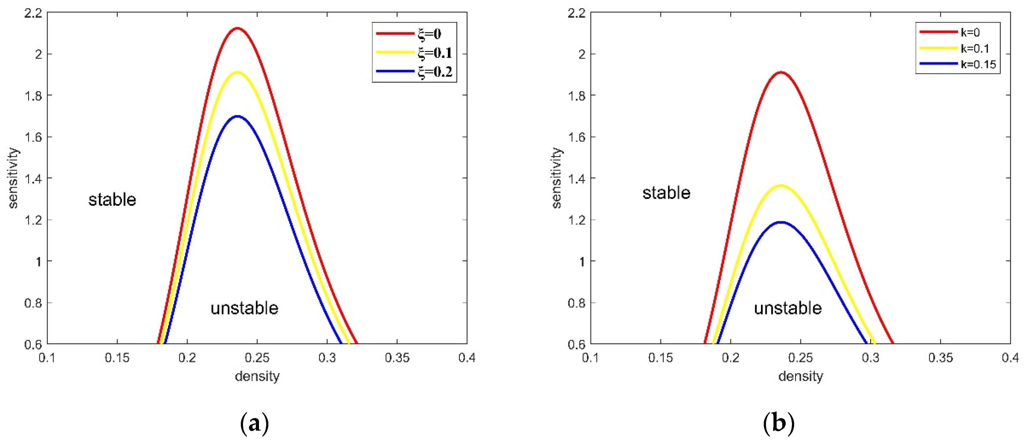
3.1. Linear Stability Analysis

The control method is properly utilized to implement the linear analysis of the novel model, and the linear stability condition is deduced in this part. To start with, the steady state of the traffic flow is displayed as the following:

$${\left[{\rho }_n,q_n\right]}^T={\left[{\rho }_n^{*},q_n^{*}\right]}^T,$$

(6)

where ${\rho }_n^{*}$ and $q_n^{*}$ are the expected density and flux, separately.

Subsequently, with the consideration of small disturbances around the steady state, the following equation is derived:

$${\partial }_t\delta {\rho }_{j+1}+{\rho }_0\left(\delta q_{j+1}-\delta q_j\right)=0,$$

(7)

$${\partial }_t\left(\delta q_j\right)=a{\rho }_0\left(1-\xi \right)\Lambda \delta {\rho }_{j+1}-a\delta q_j+ak\tau \left[{\rho }_{0}V\left({\rho }_0\right)-\delta q_j\left(t-\gamma \tau \right)\right].$$

(8)

where $\Lambda =\frac{\partial V\left({\rho }_{n+1}\right)}{\partial {\rho }_{n+1}}{|}_{{\rho }_{{}_{n+1}}={\rho }^{\ast }}$, $\delta {\rho }_j={\rho }_j-{\rho }^{\ast }$ and $\delta q_j=q_j-q^{\ast }$.

After the Laplace transform is applied, Equations (7) and (8) can be rewritten as below:

$$s{P}_{j+1}\left(s\right)-{\rho }_{j+1}\left(0\right)+{\rho }_0\left[Q_{j+1}\left(s\right)-Q_j\left(s\right)\right]=0,$$

(9)

$$s{Q}_j\left(s\right)-q_j\left(0\right)=a{\rho }_0\left(1-\xi \right)\Lambda P_{j+1}\left(s\right)-a{Q}_j\left(s\right)+ak\tau \left[\frac{1}{s}{\rho }_{0}V\left({\rho }_0\right)-e^{-s\gamma \tau }{Q}_j\left(s\right)\right].$$

(10)

where $L\left({\rho }_{j+1}\right)=P_{j+1}\left(s\right)$, $L\left(q_j\right)=Q_j\left(s\right)$ and $L\left(q_j\left(t-\gamma \tau \right)\right)=e^{-s\gamma \tau }{Q}_j\left(s\right)$.

When $P_{j+1}\left(s\right)$ in Equations (9) and (10) is eliminated, the transfer relationship can be described in the following form:

$$Q_j\left(s\right)=\frac{-a{\rho }_0^2\left(1-\xi \right)\Lambda }{p\left(s\right)}{Q}_{j+1}\left(s\right)+\frac{a{\rho }_0\left(1-\xi \right)\Lambda }{p\left(s\right)}{\rho }_{j+1}\left(0\right)+ak\tau {\rho }_{0}V\left({\rho }_0\right)+\frac{1}{p\left(s\right)}{q}_j\left(0\right).$$

(11)

where $p\left(s\right)=\left(1-ak\gamma {\tau }^2\right)s^2+a\left(1+k\tau \right)s-a{\rho }_0^2\left(1-\xi \right)\Lambda$ indicates the characteristic polynomial. Then, the transfer function $G\left(s\right)$ is acquired in accordance with Equation (11), and $G\left(s\right)$ represents the relationship between flux $Q_j$ and $Q_{j+1}$. The expression of $G\left(s\right)$ is as follows:

$$G\left(s\right)=\frac{-a{\rho }_0^2\left(1-\xi \right)\Lambda }{\left(1-ak\gamma {\tau }^2\right)s^2+a\left(1+k\tau \right)s-a{\rho }_0^2\left(1-\xi \right)\Lambda }.$$

(12)

In the control system, as long as $p\left(s\right)$ is steady and ${\Vert G\left(s\right)\Vert }_{\infty }\le 1$, traffic congestion will not take place. Based on the Hurwitz stability criterion, if all the coefficients of the quadratic polynomial $p\left(s\right)$ are greater than zero, namely, $k\le \frac{1}{a\gamma {\tau }^2}$ and $-a{\rho }_0^2(1-\xi )\Lambda >0$, we can derive that $p\left(s\right)$ is stable. Next, the process of solving the inequality ${\Vert G\left(s\right)\Vert }_{\infty }\le 1$ is given below:

$${\Vert G\left(s\right)\Vert }_{\infty }=\underset{\omega \in \left[0,\infty \right)}{\sup }\left|G\left(j\omega \right)\right|\le 1,$$

(13)

$$\left|G\left(j\omega \right)\right|=\sqrt{G\left(j\omega \right)G\left(-j\omega \right)}=\sqrt{\frac{{\left(a{\rho }_0^2\left(1-\xi \right)\Lambda \right)}^2}{{\left(\left(1-ak\gamma {\tau }^2\right){\omega }^2+a{\rho }_0^2\left(1-\xi \right)\Lambda \right)}^2+a^2{\left(1+k\tau \right)}^2{\omega }^2}}\le 1.$$

(14)

The condition of ${\Vert G\left(s\right)\Vert }_{\infty }\le 1$ is rewritten by further simplifying Equation (14), as follows:

$$2a{\rho }_0^2\left(1-\xi \right)\Lambda -2a^2{\rho }_0^2\left(1-\xi \right)\Lambda k\gamma {\tau }^2+a^2{\left(1+k\tau \right)}^2\ge 0.$$

(15)

Finally, the sufficient condition of Equation (15) can be simplified in the following form:

$$a\le \frac{-2{\rho }_0^2\left(1-\xi \right)\Lambda }{{\left(1+k\tau \right)}^2-2k\gamma {\tau }^2{\rho }_0^2\left(1-\xi \right)\Lambda }.$$

(16)

The neutral stability curves are illustrated in Figure 1, where the density–sensitivity space is separated into two parts by the curves; without satisfying the stability condition, the region below the solid line is an unstable area. Conversely, the other part, satisfying the stability condition, is the stability area. By observing Figure 1a, we could find that the stable region significantly expands when $\xi$ increases. In Figure 1b, with the rise in $k$, the unstable region declines. This means that both the strong wind and optimal flux difference integral do help to boost the enhancement of traffic flow stability, thus reducing the occurrence of traffic congestion.

3.2. Nonlinear Analysis

Aimed to acquire the mKdV equation describing the kink–antikink soliton wave, nonlinear analysis was conducted near the critical point $\left({\rho }_c,a_c\right)$. Firstly, we define the slow variables $X$ and $T$ with time $t$ and lattice $j$ in the following form:

$$X=\epsilon (j+bt),T=\epsilon t^3,0<\epsilon \ll 1,$$

(17)

where $b$ stands for an undetermined parameter. For ${\rho }_j\left(t\right)$, the following equation is satisfied:

$${\rho }_j\left(t\right)={\rho }_c+\epsilon R\left(X,T\right),$$

(18)

Employing Equations (17) and (18) to replace Equation (4), and then expanding it to the fifth order of $\epsilon$ through Taylor’s formula, we obtain the following nonlinear equation:

$$\begin{array}{l}{\epsilon }^2{k}_1{\partial }_{X}R+{\epsilon }^3{k}_2{\partial }_X^{2}R\\ +{\epsilon }^4\left[k_8{\partial }_{T}R+k_3{\partial }_X^{3}R+k_4{\partial }_X{R}^3\right]+{\epsilon }^5\left[k_5{\partial }_X{\partial }_{T}R+k_6{\partial }_X^{4}R+k_7{\partial }_X^2{R}^3\right]=0\end{array}$$

(19)

where $k_i\left(i=1,2,\cdot \cdot \cdot ,8\right)$ is elaborated in

Table 1. The coefficients $k_i$ of the new model.

$k_1$	$a\left(b+{\rho }_c^2\left(1-\xi \right)V^{\prime }({\rho }_c)+kb\tau \right)$
$k_2$	$b^2+\frac{1}{2}a{\rho }_c^2\left(1-\xi \right)V^{\prime }\left({\rho }_c\right)-\frac{1}{2}ak{b}^2{\tau }^2$
$k_3$	$\frac{1}{6}\left(a{\rho }_c^2\left(1-\xi \right)V^{\prime }\left({\rho }_c\right)+ak{b}^3{\tau }^3\right)$
$k_4$	$\frac{1}{6}a{\rho }_c^2\left(1-\xi \right)V^{‴}\left({\rho }_c\right)$
$k_5$	$2b-akb{\tau }^2$
$k_6$	$\frac{1}{24}\left({\rho }_c^2\left(1-\xi \right)V^{\prime }\left({\rho }_c\right)-b^4{\tau }^4\right)$
$k_7$	$\frac{1}{12}a{\rho }_c^2{V}^{‴}\left({\rho }_c\right)$
$k_8$	$a\left(1+k\tau \right)$

, $V^{\prime }=\frac{\partial V\left(\rho \right)}{\partial \rho }|{}_{\rho ={\rho }_c}$ and $V^{‴}=\frac{{\partial }^3{V}_0\left(\rho \right)}{\partial {\rho }^3}|{}_{\rho ={\rho }_c}$.

Using $b=-\frac{{\rho }_c^2\left(1-\xi \right)V^{\prime }\left({\rho }_c\right)}{1+k\tau }$ and $a_c=a\left(1+{\epsilon }^2\right)$, ${\epsilon }^2$ and ${\epsilon }^3$ are eliminated in Equation (19). Then, the formula can be simplified as follows:

$${\epsilon }^4\left(g_1{\partial }_X^{3}R+g_2{\partial }_X{R}^3+{\partial }_{T}R\right)+{\epsilon }^5\left(g_4{\partial }_X^{4}R+g_5{\partial }_X^2{R}^3+g_3{\partial }_X^{2}R\right)=0,$$

(20)

where $g_i\left(i=1,2,\cdots ,8\right)$ is elaborated in

Table 2. The coefficients $g_i$ of the new model.

$g_1$	$\frac{1}{6}\left(a{\rho }_c^2\left(1-\xi \right)V^{\prime }\left({\rho }_c\right)+ak{b}^3{\tau }^3\right)$
$g_2$	$\frac{1}{6}a{\rho }_c^2\left(1-\xi \right)V^{‴}\left({\rho }_c\right)$
$g_3$	$\frac{{\rho }_c^4{\left(1-\xi \right)}^2{V^{\prime }}^2\left({\rho }_c\right)}{{\left(1+k\tau \right)}^2}$
$g_4$	$\frac{1}{24}\left(a{\rho }_c^2\left(1-\xi \right)V^{\prime }\left({\rho }_c\right)-b^4{\tau }^4\right)$
$g_5$	$\frac{1}{12}a{\rho }_c^2\left(1-\xi \right)V^{‴}\left({\rho }_c\right)$

.

After Equation (20) is transformed with $T=\frac{1}{g_1}{T}^{\prime },R=\sqrt{\frac{g_1}{g_2}}{R}^{\prime }$, the regularized mKdV equation that has the correction term $O(\epsilon )$, is obtained:

$${\partial }_{T^{\prime }}{R}^{\prime }={\partial }_X^3{R}^{\prime }-{\partial }_X{R^{\prime }}^3+\epsilon \left[\frac{g_3}{g_1}{\partial }_X^2{R}^{\prime }+\frac{g_4}{g_1}{\partial }_X^4{R}^{\prime }+\frac{g_5}{g_2}{\partial }_X^2{R^{\prime }}^3\right],$$

(21)

When the $O(\epsilon )$ is ignored, the regularized mKdV equation can be obtained, and its soliton solution is as follows:

$${R^{\prime }}_o\left(X,T^{\prime }\right)=\sqrt{c}\tanh \sqrt{\frac{c}{2}}\left(X-c{T}^{\prime }\right).$$

(22)

To derive the propagation velocity $c$ in Equation (22), the equation $R^{\prime }\left(X,T^{\prime }\right)={R^{\prime }}_o\left(X,T^{\prime }\right)+\epsilon {R^{\prime }}_1\left(X,T^{\prime }\right)$ is presumed, and the solvability condition given below must be satisfied:

$$\left({R^{\prime }}_o,M\left[{R^{\prime }}_o\right]\right)\equiv {\displaystyle {\int }_{-\infty }^{+\infty }d{X}^{\prime }}{R^{\prime }}_{o}M\left[{R^{\prime }}_o\right]=0,$$

(23)

where $M\left[{R^{\prime }}_o\right]=\frac{g_3}{g_1}{\partial }_X^2{R}^{\prime }+\frac{g_4}{g_1}{\partial }_X^4{R}^{\prime }+\frac{g_5}{g_2}{\partial }_X^2{R^{\prime }}^3$. Consequently, we acquire the general speed $c$, shown as follows:

$$c=\frac{5g_2{g}_3}{2g_2{g}_4-3g_1{g}_5}.$$

(24)

Then, utilizing $T=\frac{1}{g_1}{T}^{\prime }$ and $R=\sqrt{\frac{g_1}{g_2}}{R}^{\prime }$ for substitution in Equation (22), the expression of $R\left(X,T\right)$ is shown as follows:

$$R\left(X,T\right)=\sqrt{\frac{g_{1}c}{g_2}}\tanh \left(\sqrt{\frac{c}{2}}\left(X-c{g}_{1}T\right)\right).$$

(25)

Eventually, the general solution of the kink–antikink soliton of the density wave is deduced by inserting Equation (25) into Equation (18), as follows:

$${\rho }_j(t)={\rho }_c+\epsilon \sqrt{\frac{g_{1}c}{g_2}}\tanh \left(\sqrt{\frac{c}{2}}(X-c{g}_{1}T)\right),$$

(26)

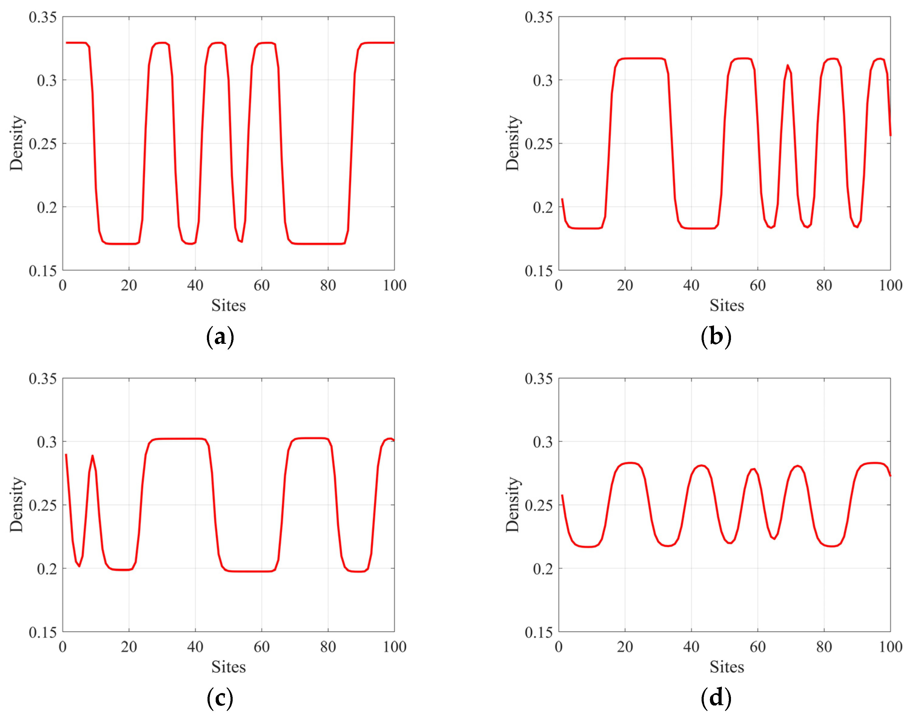
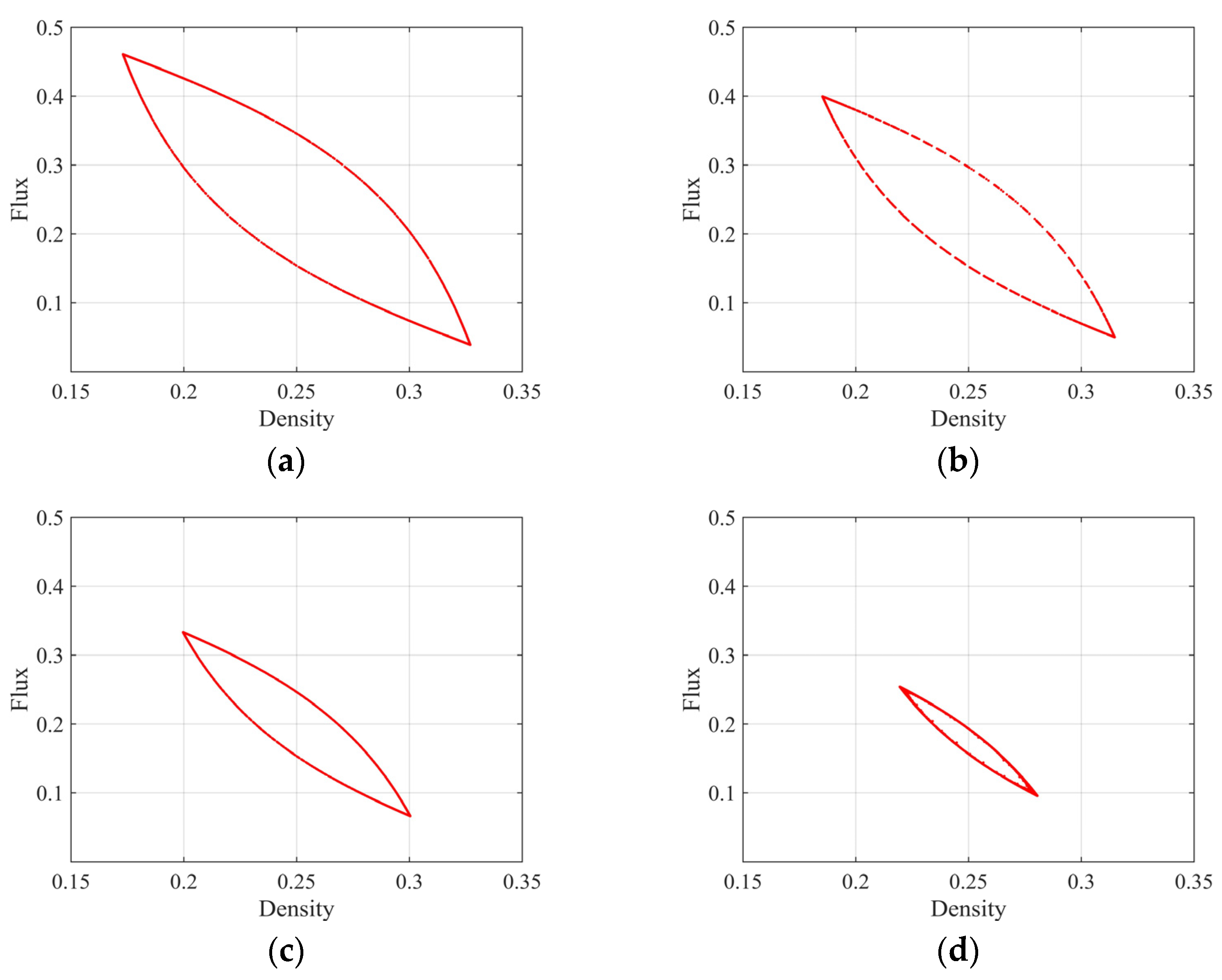
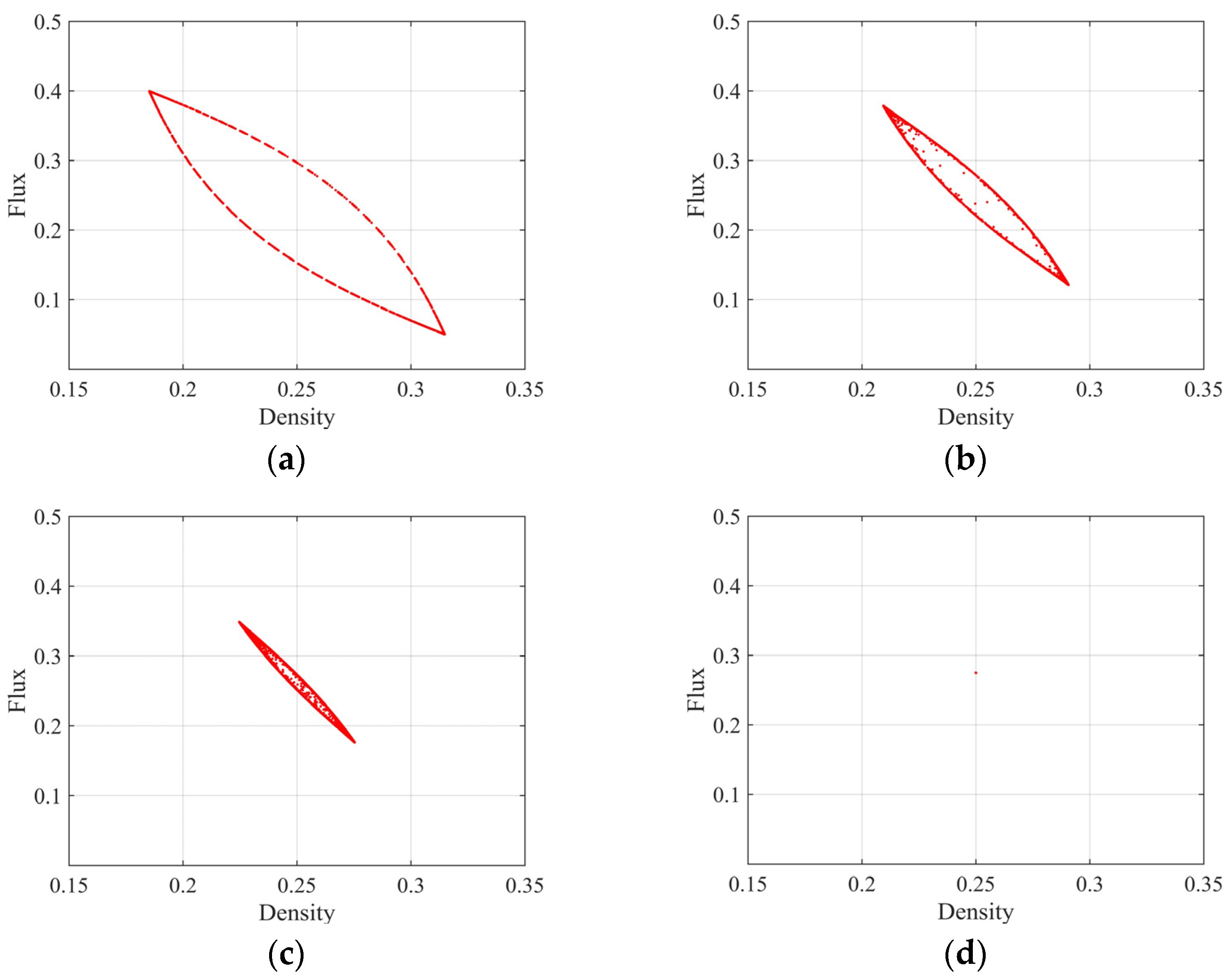
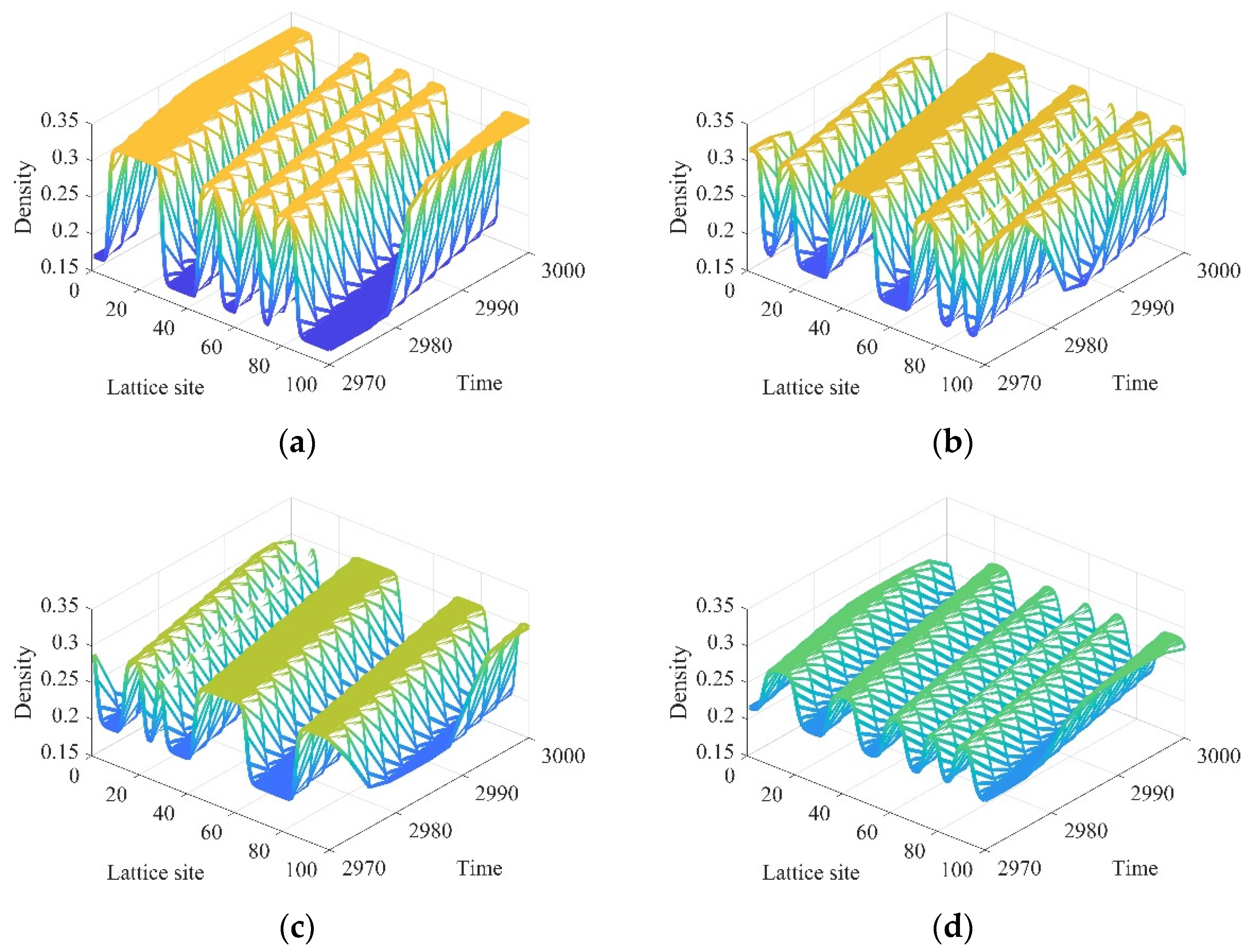
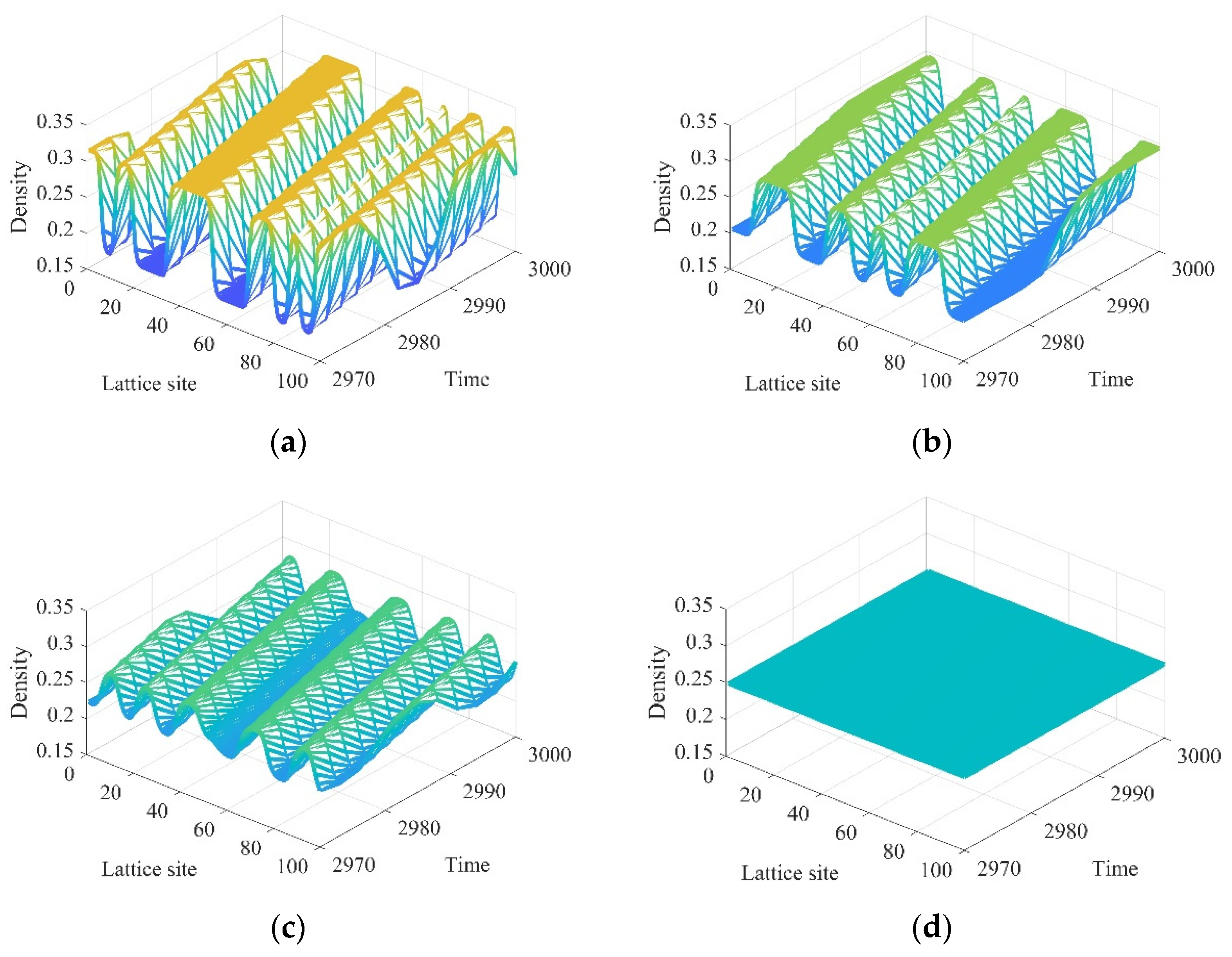
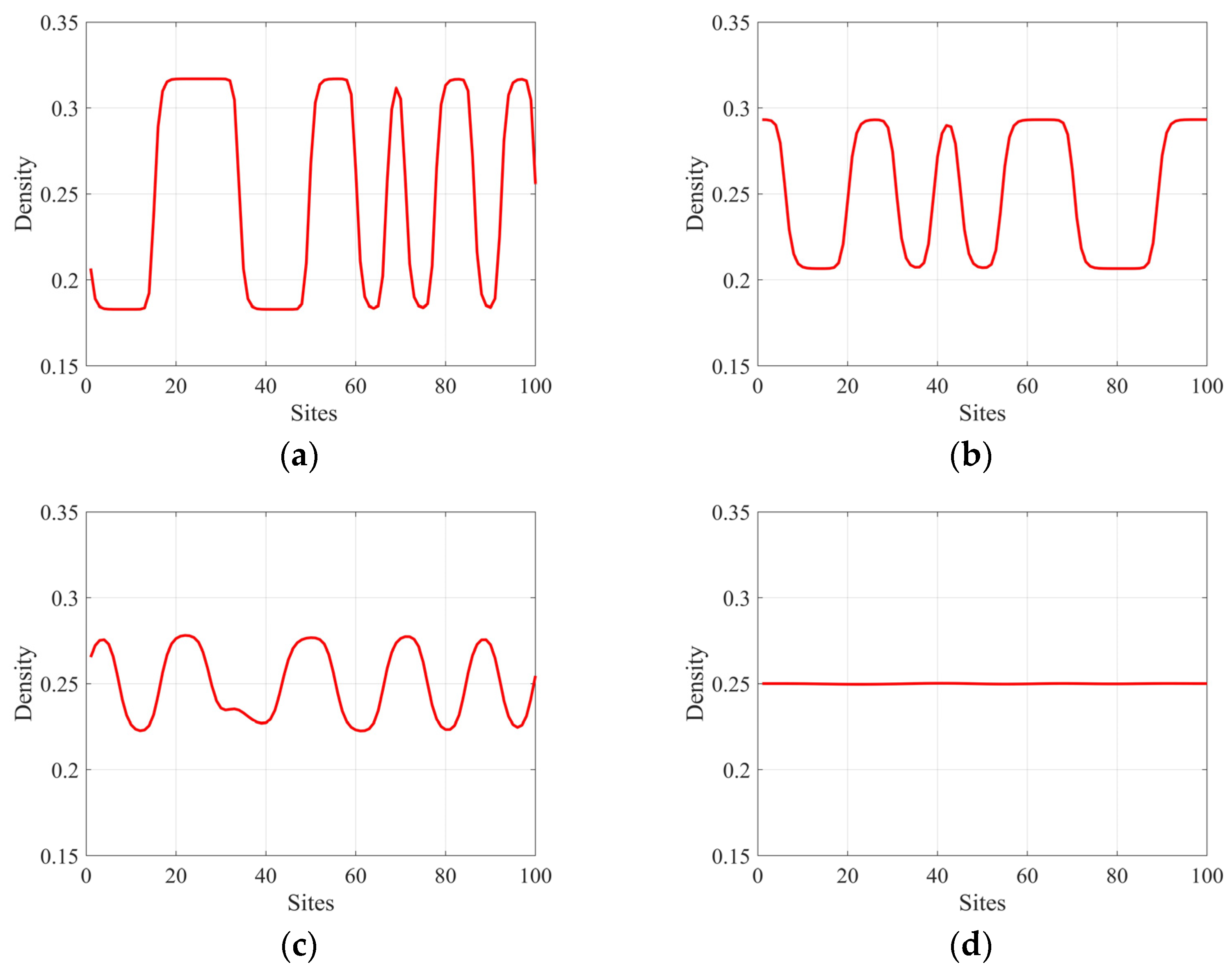
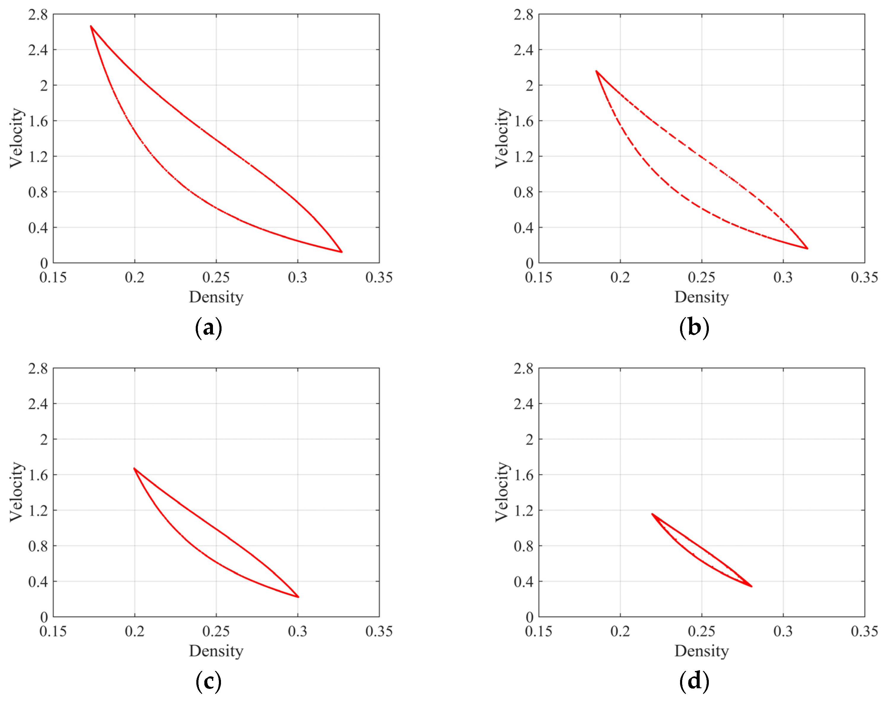
4. Results of Numerical Simulation

To investigate the effect of strong wind and optimal estimation of flux difference integral, numerical simulation is conducted on the proposed model. We choose $N=100$, signifying the total number of sites, and the original conditions for the new model are given as follows:

$${\rho }_j\left(1\right)={\rho }_j(0)=\{\begin{array}{ll}{\rho }_0,\hfill & j\ne \frac{N}{2},\frac{N}{2}+1,\hfill \\ {\rho }_0-0.05,\hfill & j=\frac{N}{2},\hfill \\ {\rho }_0+0.05,\hfill & j=\frac{N}{2}+1.\hfill \end{array},$$

(27)

where ${\rho }_0={\rho }_c=0.25$, $a=1.3$, $t=3000$, and $v_{\max }=2$.

Figure 2 and Figure 3 only consider the effect of strong wind, whereas Figure 2 illustrates the space-time evolution of the densities for $\xi =0,0.1,0.2,0.3$, severally. With the rise in the value of $\xi$, the amplitude of the curve decreases. In Figure 3, the density profile at time $t=3000s$, with different $\xi$, is demonstrated. Comparing the patterns from (a) to (d) in Figure 3, it could be discovered that the fluctuation amplitude of the curves obviously declines. Based on the figures above, when the wind force becomes stronger and stronger, the traffic flow tends to be more stable, to some extent. That is to say, the strong wind is conducive to stabilizing the traffic flow.

Then, we further consider the control signal on the grounds of accounting for the strong wind. The simulation result is given in Figure 4 and Figure 5.

Figure 4 represents the space-time evolution of the densities for different coefficients $k=0,0.1,0.15,0.2$, where $\xi =0.1$. Figure 5 depicts the density profile at time $t=3000s$, corresponding to Figure 4. From the two figures, we know that the oscillation amplitude of the density wave lessens with the rise in $k$. In view of the results, traffic flow becomes steadier when the control signal is taken into consideration.

In the congested areas, driving must become very difficult, and drivers have to accelerate or decelerate to alter the condition of the traffic. Diverse traffic flow state paths of acceleration or deceleration would result in the hysteresis phenomenon, which is demonstrated not only in the flux–density diagram, but also in the velocity–density diagram.

Figure 6 and Figure 7 show the hysteresis loops of traffic flux and density, and the hysteresis loops of velocity and density, respectively, under the influence of strong wind. A similarity between the two figures is that the size of the hysteresis loop decreases with the rise in coefficient $\xi$. The above phenomenon reflects that the stability of traffic flow has been enhanced.

Then, we fix the coefficient $\xi$ and further consider the feedback control. The corresponding hysteresis loops are shown in Figure 8 and Figure 9. The hysteresis loop narrows to a point, indicating that traffic congestion was largely absent at the moment when the value $k$ increased to 0.2.

5. Conclusions

The impact of strong wind and optimal flux difference integral are incorporated in a new model, and the influence of the two factors on traffic flow has been investigated through linear analysis, as well as nonlinear analysis, in this paper. In the linear analysis, the stability condition was obtained by utilization of the control method. The mKdV equation, which describes the propagating features of traffic density waves, is acquired via nonlinear analysis. Then, numerical simulation carried out on the new model revealed that the optimal flux difference integral avails to stabilize the traffic flow. Moreover, to a certain extent, the traffic flow becomes more stable with the increase in strong wind. The simulation presents the same results as the theoretical analysis. Hence, the model proposed in this study is conducive to understanding the underlying mechanism of traffic congestion, thus alleviating traffic jams.

References

1. Ma, C.; Wei, H.; He, R. Distribution path robust optimization of electric vehicle with multiple distribution centers. PLoS ONE 2018, 13, e0193789. [Google Scholar]
2. Ma, C.; Wei, H.; Pan, F. Road screening and distribution route multi-objective robust optimization for hazardous materials based on neural network and genetic algorithm. PLoS ONE 2018, 13, e0198931. [Google Scholar]
3. Ma, C.; He, R.; Zhang, W. Path optimization of taxi carpooling. PLoS ONE 2018, 13, e0203221. [Google Scholar]
4. Ma, C.; Wei, H.; Wang, A. Developing a coordinated signal control system for urban ring road under the vehicle-infrastructure connected environment. IEEE Access 2018, 6, 52471–52478. [Google Scholar] [CrossRef]
5. Tang, T.; Luo, X.; Zhang, J.; Chen, L. Modeling electric bicycle’s lane-changing and retrograde behaviors. Phys. A 2018, 490, 1377–1386. [Google Scholar] [CrossRef]
6. Tang, T.; Zhang, J.; Liu, K. A speed guidance model accounting for the driver’s bounded rationality at a signalized intersection. Phys. A 2017, 473, 45–52. [Google Scholar] [CrossRef]
7. Wu, X.; Zhao, X.; Song, H. Effects of the prevision relative velocity on traffic dynamics in the ACC strategy. Phys. A 2019, 515, 192–198. [Google Scholar] [CrossRef]
8. Tang, T.; Shi, W.; Huang, H. A route-based traffic flow model accounting for interruption factors. Phys. A 2019, 514, 767–785. [Google Scholar] [CrossRef]
9. Guo, Y.; Xue, Y.; Shi, Y. Mean-field velocity difference model considering the average effect of multi-vehicle interaction. Commun. Nonlinear Sci. Numer. Simul. 2018, 59, 553–564. [Google Scholar] [CrossRef]
10. Zhu, W.; Jun, D.; Zhang, L. A compound compensation method for car-following model. Commun. Nonlinear Sci. Numer. Simul. 2016, 39, 427–441. [Google Scholar] [CrossRef]
11. Bando, M.; Hasebe, K.; Nakayama, A. Dynamical model of traffic congestion and numerical simulation. Phys. Rev. E 1995, 51, 1035–1042. [Google Scholar] [CrossRef] [PubMed]
12. Zhu, W.; Zhang, L. Analysis of car-following model with cascade compensation strategy. Phys. A 2016, 449, 265–274. [Google Scholar] [CrossRef]
13. Zhu, W.; Zhang, H. Analysis of mixed traffic flow with human-driving and autonomous cars based on car-following model. Phys. A 2018, 496, 274–285. [Google Scholar] [CrossRef]
14. Wang, J.; Sun, F.; Ge, H. Effect of the driver’s desire for smooth driving on the car-following model. Phys. A 2018, 512, 96–108. [Google Scholar] [CrossRef]
15. Zhu, W.; Zhang, L. A new car-following model for autonomous vehicles flow with mean expected velocity field. Phys. A 2018, 492, 2154–2165. [Google Scholar]
16. Sun, Y.; Ge, H.; Cheng, R. An extended car-following model under V2V communication environment and its delayed-feedback control. Phys. A 2018, 508, 349–358. [Google Scholar] [CrossRef]
17. Sun, Y.; Ge, H.; Cheng, R. An extended car-following model considering drivers memory and average speed of preceding vehicles with control strategy. Phys. A 2019, 521, 752–761. [Google Scholar] [CrossRef]
18. Wang, T.; Cheng, R.; Ge, H. An extended two-lane lattice hydrodynamic model for traffic flow on curved road with passing. Phys. A 2019, 533, 121915. [Google Scholar] [CrossRef]
19. Ou, H.; Tang, T. An extended two-lane car-following model accounting for inter-vehicle communication. Phys. A 2018, 495, 260–268. [Google Scholar] [CrossRef]
20. Xin, Q.; Yang, N.; Fu, R. Impacts analysis of car following models considering variable vehicular gap policies. Phys. A 2018, 501, 338–355. [Google Scholar] [CrossRef]
21. Tang, T.; Rui, Y.; Zhang, J.; Shang, H. A cellular automation model accounting for bicycle’s group behavior. Phys. A 2018, 492, 1782–1797. [Google Scholar] [CrossRef]
22. Xue, Y.; Dong, L.; Dai, S. An improved one-dimensional cellular automaton model of traffic flow and the effect of deceleration probability. Acta Phys. Sin. 2001, 50, 445–449. [Google Scholar] [CrossRef]
23. Gao, K.; Jiang, R.; Hu, S.; Wang, B.; Wu, Q. Cellular-automaton model with velocity adaptation in the framework of Kerner’s three-phase traffic theory. Phys. Rev. E 2007, 76, 026105. [Google Scholar] [CrossRef] [PubMed]
24. Cheng, R.; Ge, H.; Wang, J. The nonlinear analysis for a new continuum model considering anticipation and traffic jerk effect. Appl. Math. Comput. 2018, 332, 493–505. [Google Scholar]
25. Cheng, R.; Ge, H.; Wang, J. KdV-Burgers equation in a new continuum model based on full velocity difference model considering anticipation effect. Phys. A 2017, 481, 52–59. [Google Scholar] [CrossRef]
26. Cheng, R.; Ge, H.; Wang, J. An extended continuum model accounting for the driver’s timid and aggressive attributions. Phys. Lett. A 2017, 381, 1302–1312. [Google Scholar] [CrossRef]
27. Zhai, Q.; Ge, H.; Cheng, R. An extended continuum model considering optimal velocity change with memory and numerical tests. Phys. A 2018, 490, 774–785. [Google Scholar]
28. Cheng, R.; Wang, Y. An extended lattice hydrodynamic model considering the delayed feedback control on a curved road. Phys. A 2019, 513, 510–517. [Google Scholar] [CrossRef]
29. Kaur, R.; Sharma, S. Modeling and simulation of driver’s anticipation effect in a two lane system on curved road with slope. Phys. A 2018, 499, 110–120. [Google Scholar] [CrossRef]
30. Jiang, C.; Cheng, R.; Ge, H. Mean-field flow difference model with consideration of on-ramp and off-ramp. Phys. A 2019, 513, 465–476. [Google Scholar] [CrossRef]
31. Jiang, C.; Cheng, R.; Ge, H. An improved lattice hydrodynamic model considering the “backward looking” effect and the traffic interruption probability. Nonlinear Dyn. 2017, 91, 777–784. [Google Scholar] [CrossRef]
32. Kaur, R.; Sharma, S. Analyses of a heterogeneous lattice hydrodynamic model with low and high-sensitivity vehicles. Phys. Lett. A 2018, 382, 1449–1455. [Google Scholar] [CrossRef]
33. Peng, G.; Kuang, H.; Qing, L. A new lattice model of traffic flow considering driver’s anticipation effect of the traffic interruption. Phys. A 2018, 507, 374–380. [Google Scholar] [CrossRef]
34. Wang, Q.; Ge, H. An improved lattice hydrodynamic model accounting for the effect of “backward looking” and flow integral. Phys. A 2019, 513, 438–446. [Google Scholar] [CrossRef]
35. Redhu, P.; Gupta, A. Delayed-feedback control in a lattice hydrodynamic model. Commun. Nonlinear Sci. Numer. Simul. 2015, 27, 263–270. [Google Scholar] [CrossRef]
36. Qin, S.; Ge, H.; Cheng, R. A new lattice hydrodynamic model based on control method considering the flux change rate and delay feedback signal. Phys. Lett. A 2018, 382, 482–488. [Google Scholar] [CrossRef]
37. Chang, Y.; He, Z.; Cheng, R. An extended lattice hydrodynamic model considering the driver’s sensory memory and delayed-feedback control. Phys. A 2019, 514, 522–532. [Google Scholar] [CrossRef]
38. Peng, G.; Zhao, H.; Liu, X. The impact of self-stabilization on traffic stability considering the current lattice’s historic flux for two-lane freeway. Phys. A 2019, 515, 31–37. [Google Scholar] [CrossRef]
39. Nagatani, T. Modified KdV equation for jamming transition in the continuum models of traffic. Phys. A 1998, 261, 599–607. [Google Scholar] [CrossRef]
40. Tian, J.; Yuan, Z.; Jia, B.; Li, M.; Jiang, G. The stabilization effect of the density difference in the modified lattice hydrodynamic model of traffic flow. Phys. A 2012, 391, 4476–4482. [Google Scholar] [CrossRef]
41. Zhao, H.; Zhang, G.; Li, W.; Gu, T.; Zhou, D. Lattice hydrodynamic modeling of traffic flow with consideration of historical current integration effect. Phys. A 2018, 503, 1204–1211. [Google Scholar] [CrossRef]
42. Sharma, S. Modeling and analyses of drivers characteristics in a traffic system with passing. Nonlinear Dyn. 2016, 86, 2093–2104. [Google Scholar] [CrossRef]
43. Wang, J.; Sun, F.; Ge, H. An improved lattice hydrodynamic model considering the driver’s desire of driving smoothly. Phys. A 2019, 515, 119–129. [Google Scholar] [CrossRef]
44. Kwon, S.; Kim, D.; Lee, S. Deisgn criteria of wind barriers for traffic. part 1: Wind barrier performance. Wind Struct. 2011, 14, 55–70. [Google Scholar] [CrossRef] [Green Version]
45. Liu, D.; Shi, Z.; Ai, W. An improved car-following model accounting for impact of strong wind. Math. Probl. Eng. 2017, 2017, 4936490. [Google Scholar] [CrossRef] [Green Version]
46. Yang, S.; Li, C.; Tang, X.; Tian, C. Effect of optimal estimation of flux difference information on the lattice traffic flow model. Phys. A 2016, 463, 394–399. [Google Scholar] [CrossRef]
47. Peng, G.; Yang, S.; Xia, D.; Li, X. A novel lattice hydrodynamic model considering the optimal estimation of flux difference effect on two-lane highway. Phys. A 2018, 506, 929–937. [Google Scholar] [CrossRef]
48. Ge, H.; Cui, Y.; Zhu, K.; Cheng, R. The control method for the lattice hydrodynamic model. Commun. Nonlinear Sci. Numer. Simul. 2015, 22, 903–908. [Google Scholar] [CrossRef]
49. Zhu, C.; Zhong, S.; Li, G.; Ma, S. New control strategy for the lattice hydrodynamic model of traffic flow. Phys. A 2017, 468, 445–453. [Google Scholar] [CrossRef]
Figure 1. Phase diagram in parameter space ( ρ , α ) . (a) k = 0 , (b)   ξ = 0.1 .
Mathematics 09 02897 g001
Figure 2. The evolution of the traffic densities for different values of parameter ξ . (a) ξ = 0 , (b) ξ = 0.1 , (c) ξ = 0.2 , (d) ξ = 0.3 .
Mathematics 09 02897 g002
Figure 3. The density profile at t = 3000 s under the different values of ξ . (a) ξ = 0 , (b) ξ = 0.1 , (c) ξ = 0.2 , (d) ξ = 0.3 .
Mathematics 09 02897 g003
Figure 4. The evolution of the traffic flux for different values of parameter k . (a) k = 0 , (b) k = 0.1 , (c) k = 0.15 , (d) k = 0.2 .
Mathematics 09 02897 g004
Figure 5. The flux profile at t = 3000 s under the different value of k . (a) k = 0 , (b) k = 0.1 , (c) k = 0.15 , (d) k = 0.2 .
Mathematics 09 02897 g005
Figure 6. The hysteresis loops of traffic flux and density for different ξ . (a) ξ = 0 , (b) ξ = 0.1 , (c) ξ = 0.2 , (d) ξ = 0.3 .
Mathematics 09 02897 g006
Figure 7. The hysteresis loops of velocity and density for different ξ . (a) ξ = 0 , (b) ξ = 0.1 , (c) ξ = 0.2 , (d) ξ = 0.3 .
Mathematics 09 02897 g007
Figure 8. The hysteresis loops of traffic flux and density for different k . (a) k = 0 , (b) k = 0.1 , (c) k = 0.15 , (d) k = 0.2 .
Mathematics 09 02897 g008
Figure 9. The hysteresis loops of velocity and density for different k . (a) k = 0 , (b) k = 0.1 , (c) k = 0.15 , (d) k = 0.2 .
Mathematics 09 02897 g009