
The Improved Element-Free Galerkin Method for 3D Helmholtz Equations


Abstract
:1. Introduction
2. The IMLS Approximation
3. The IEFG Method for 3D Helmholtz Equations
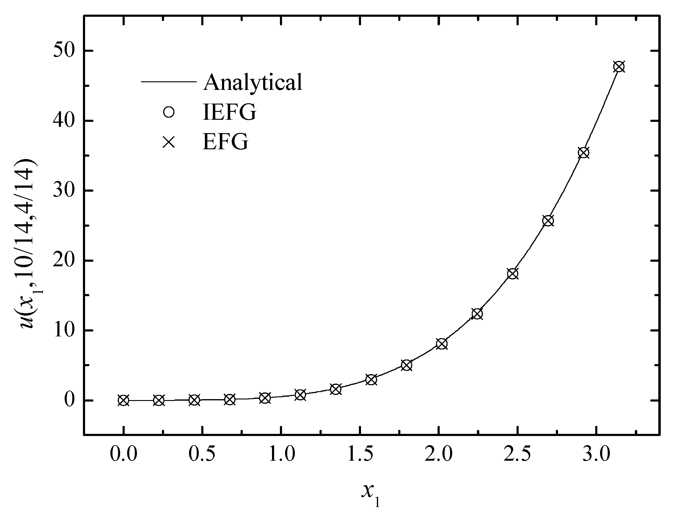
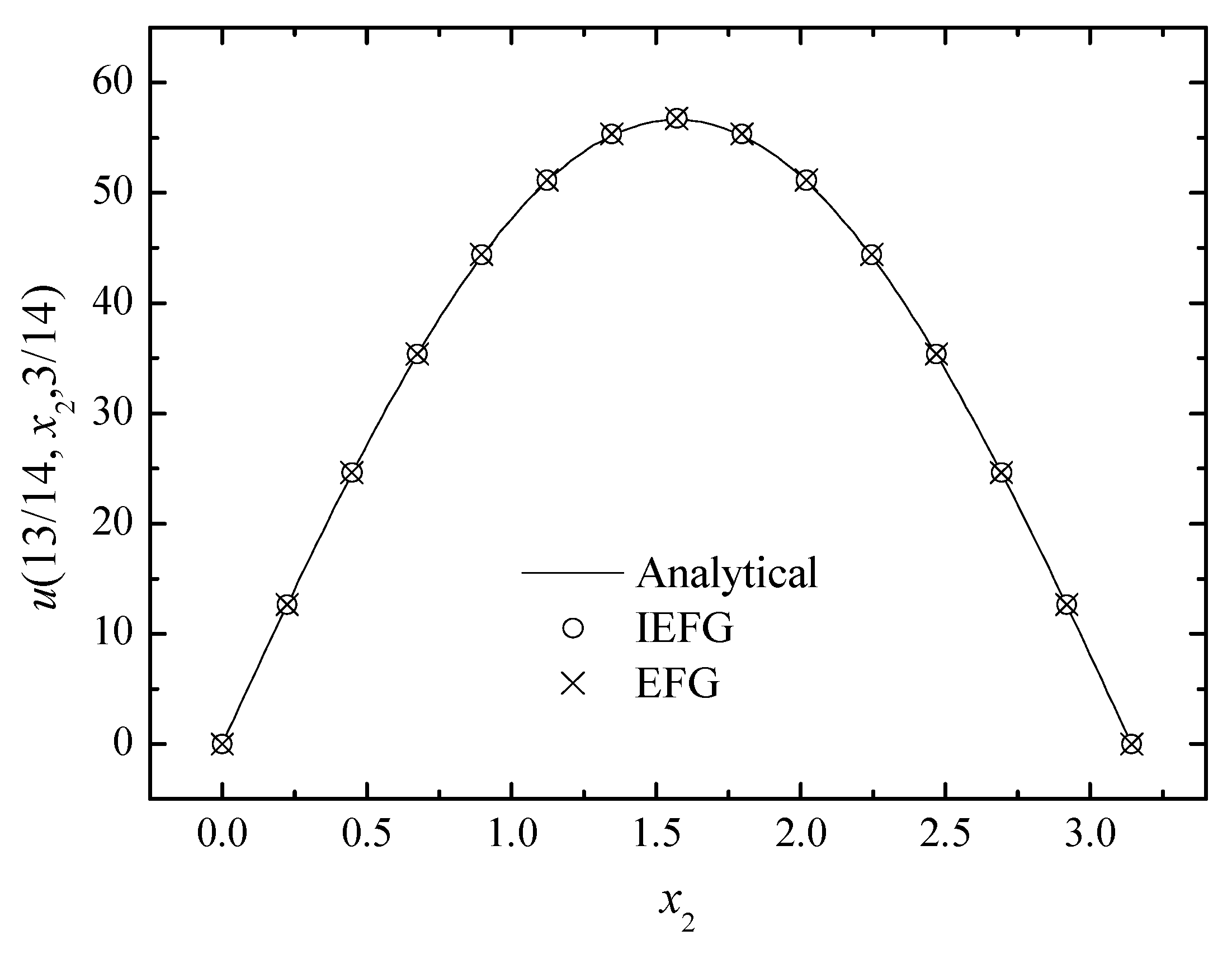
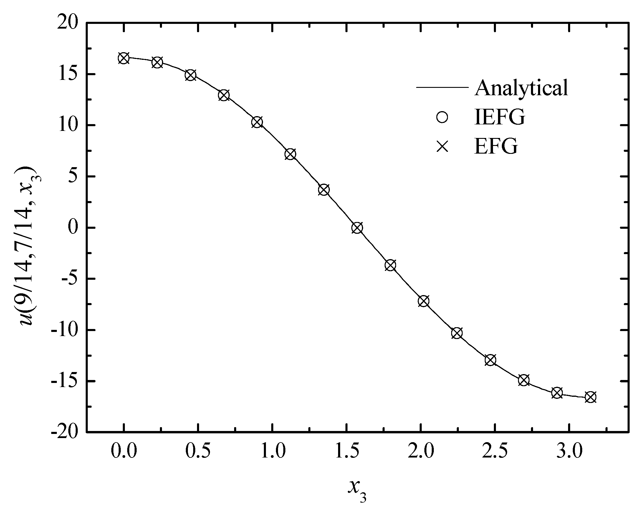
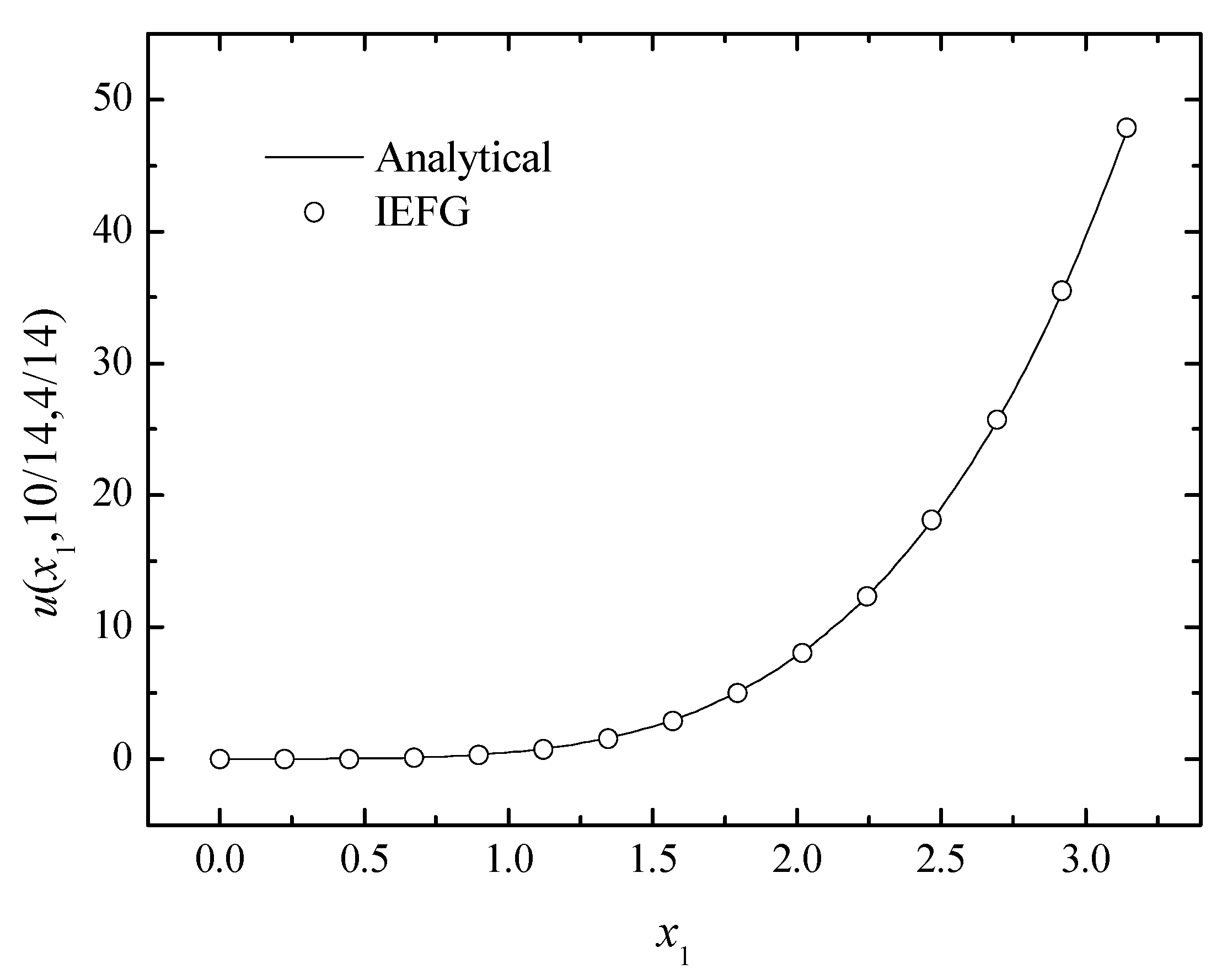
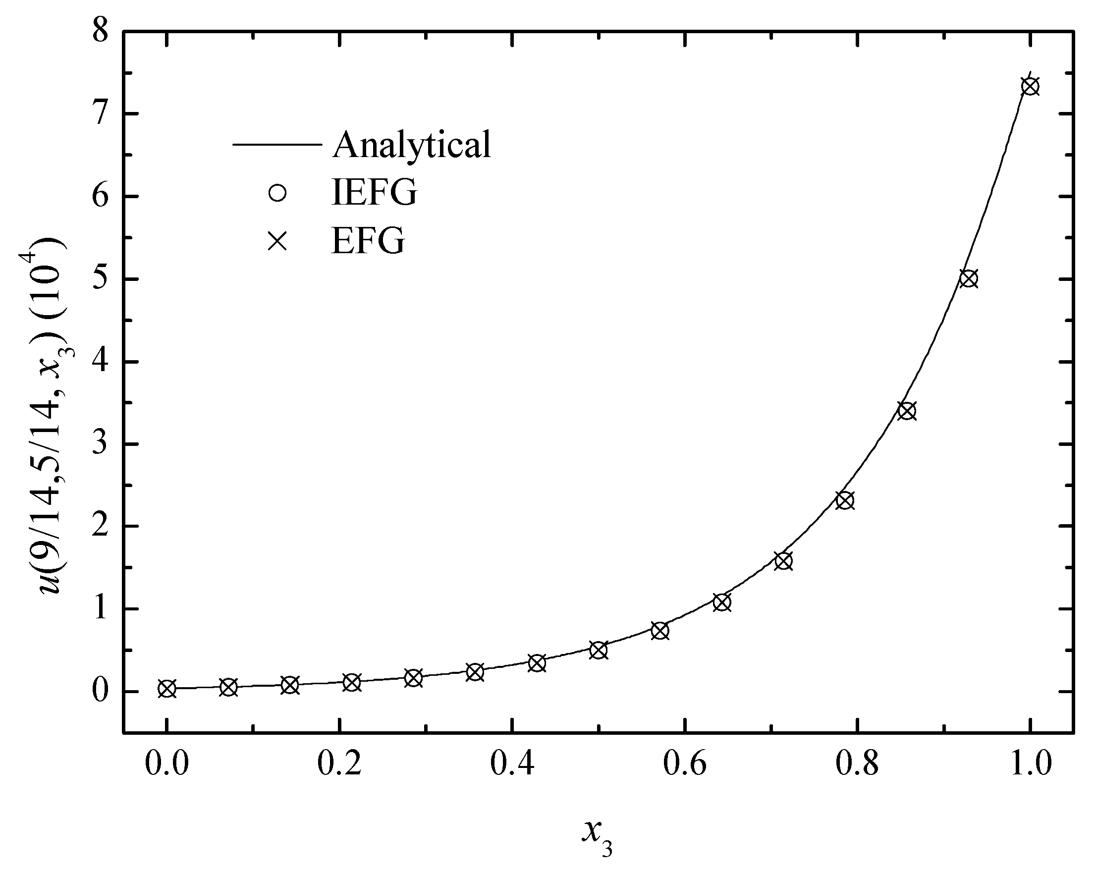
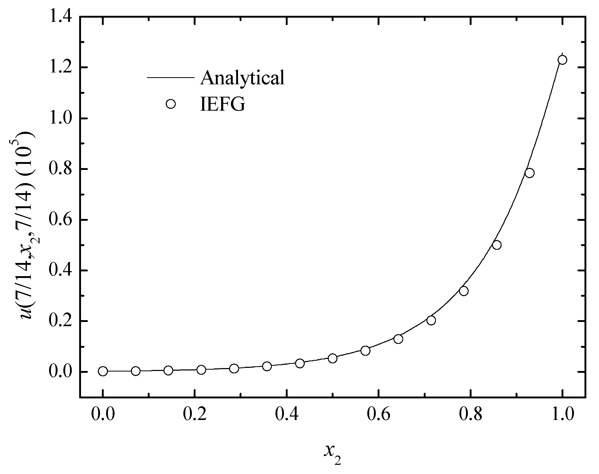
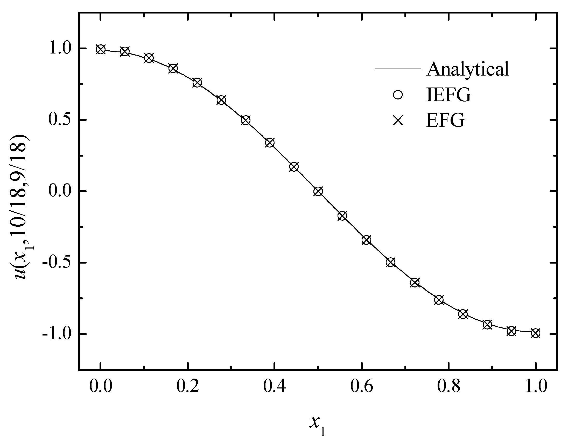
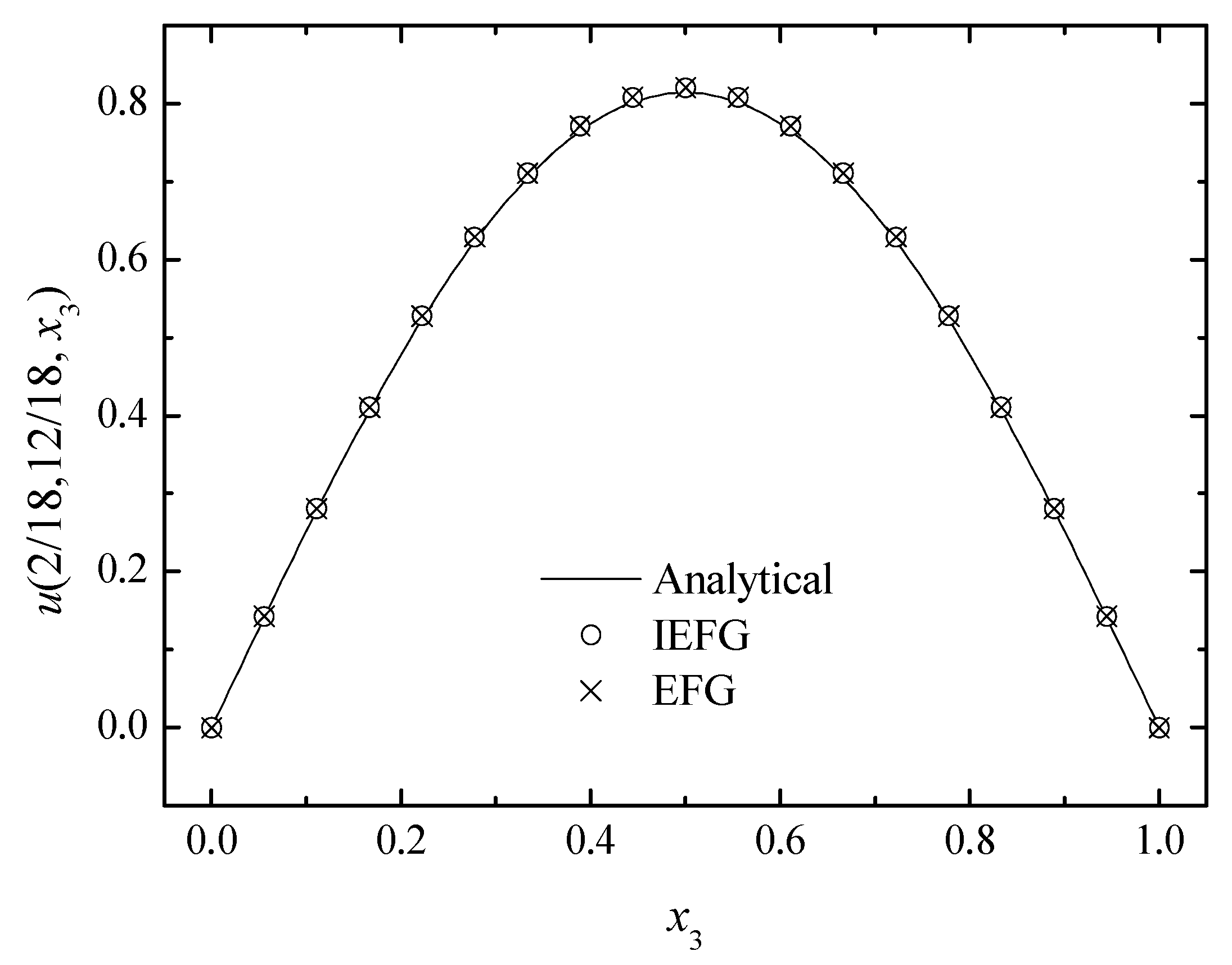
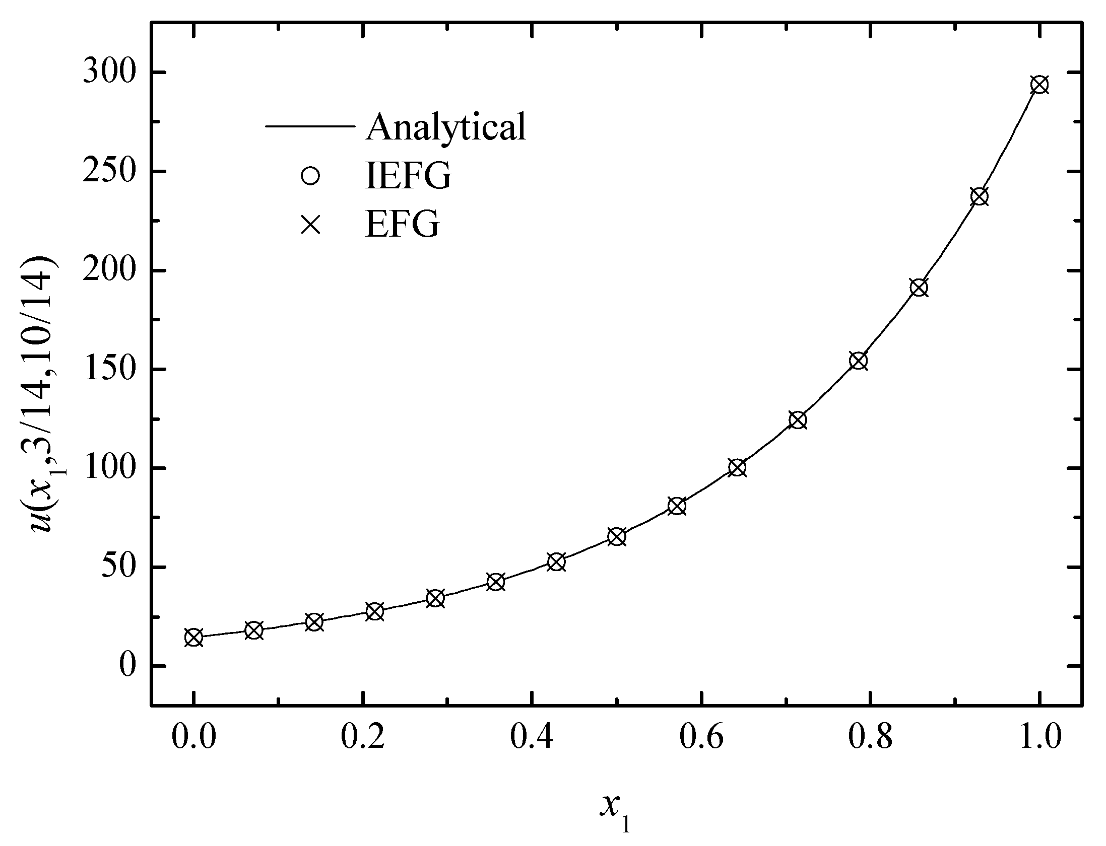
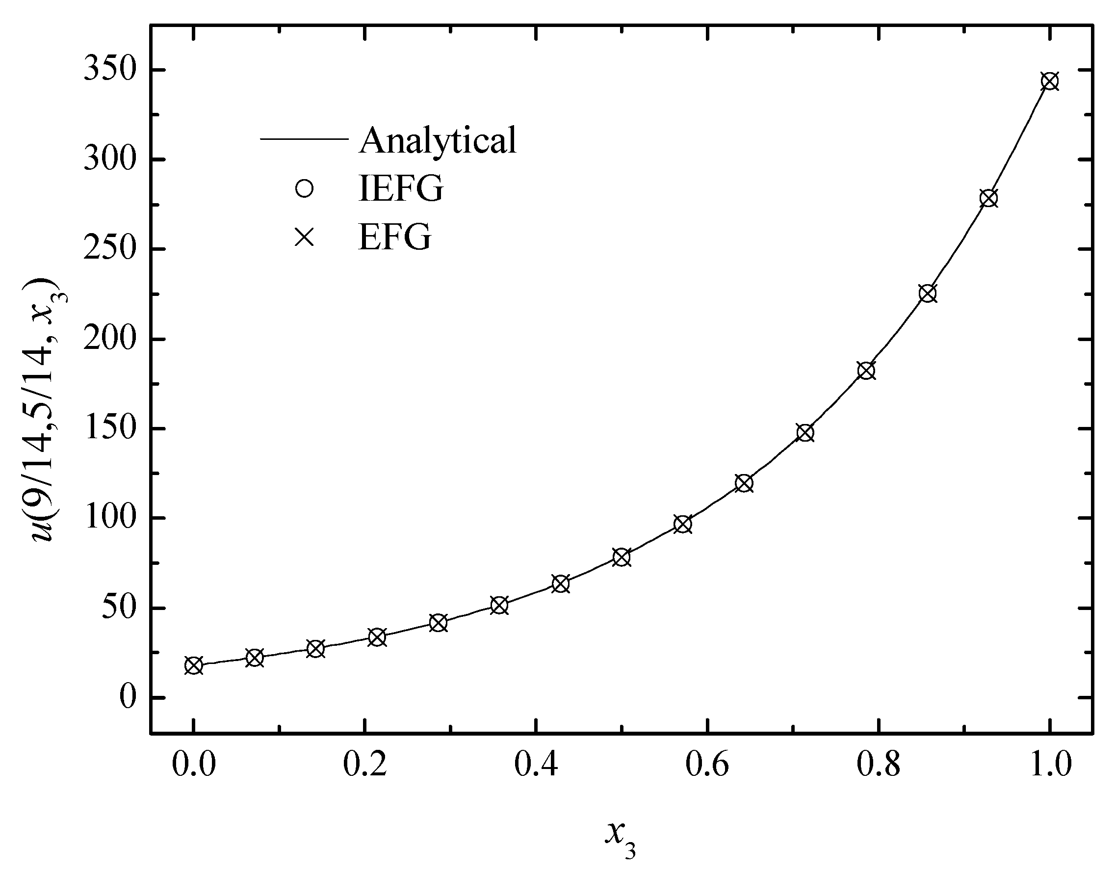
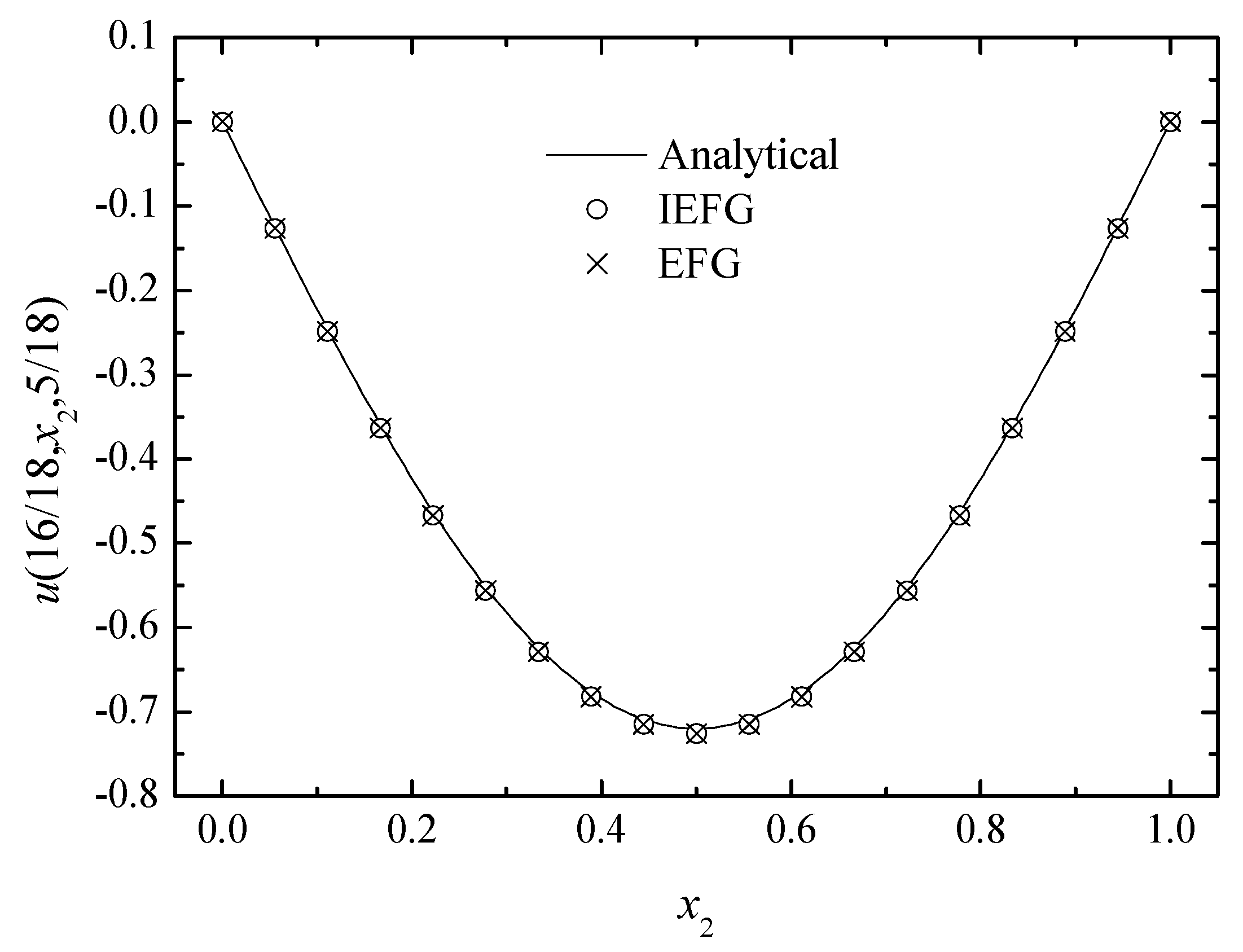
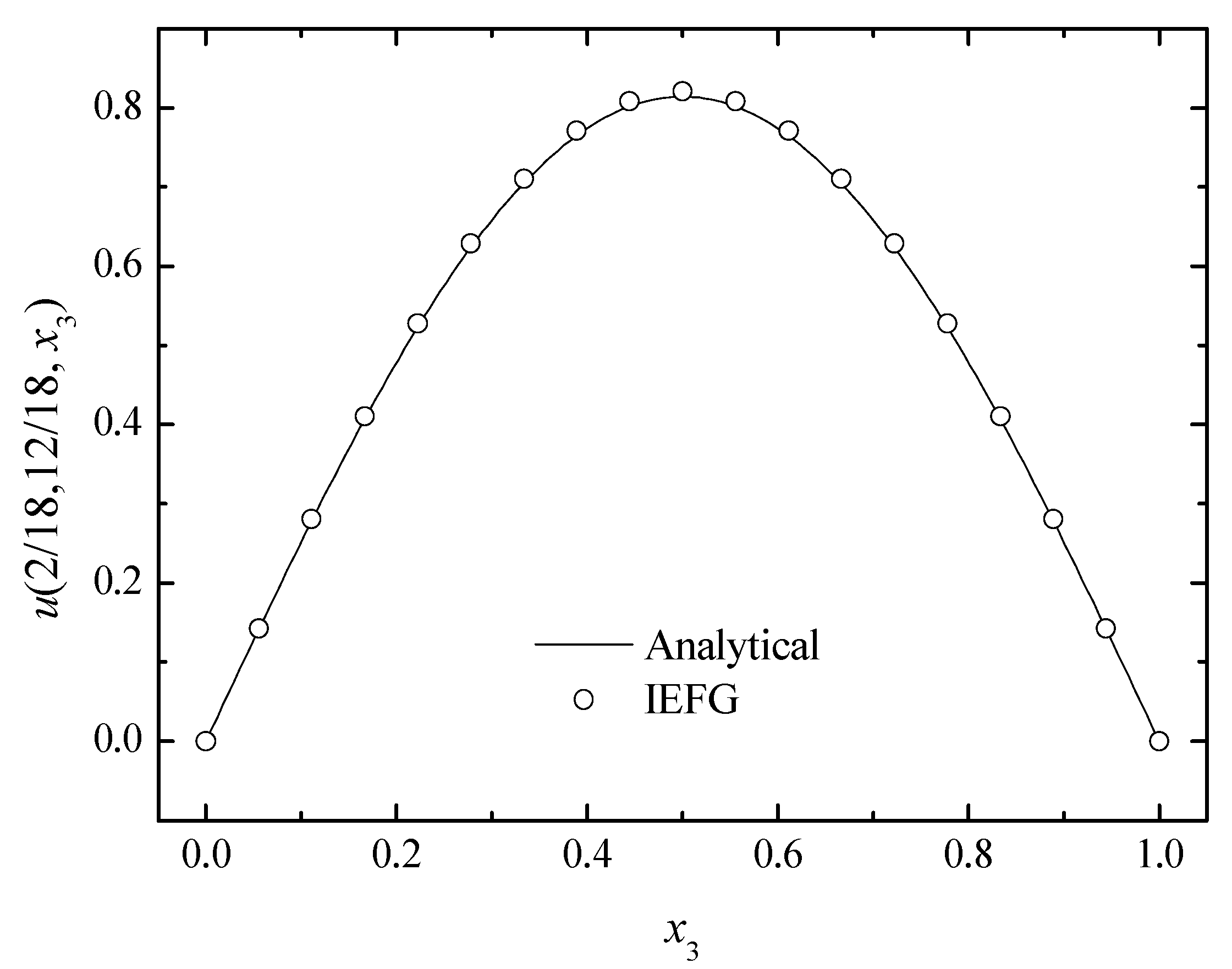
4. Numerical Examples
- (1)
- Weight function
- (2)
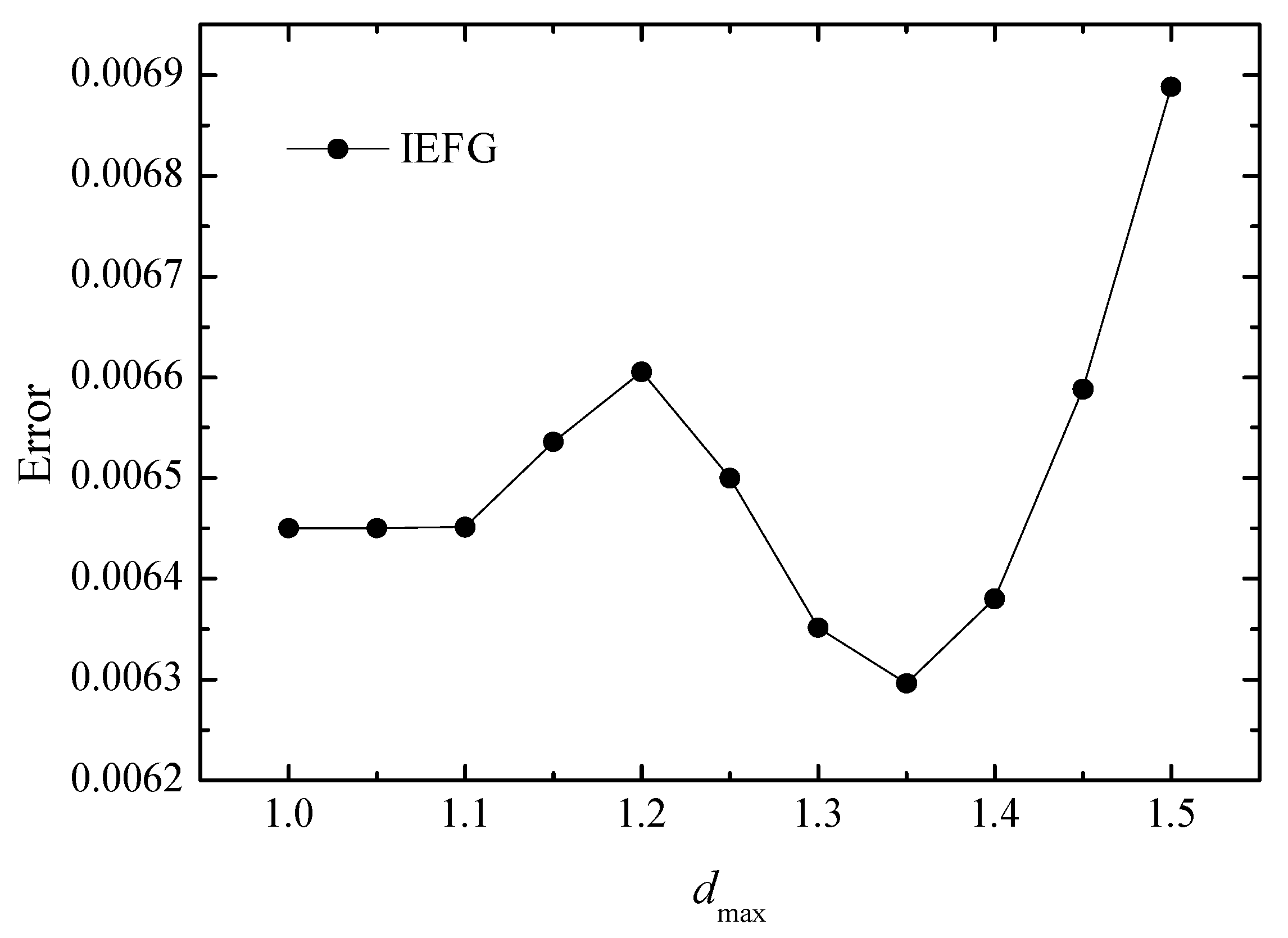
- Scale parameter
- (3)
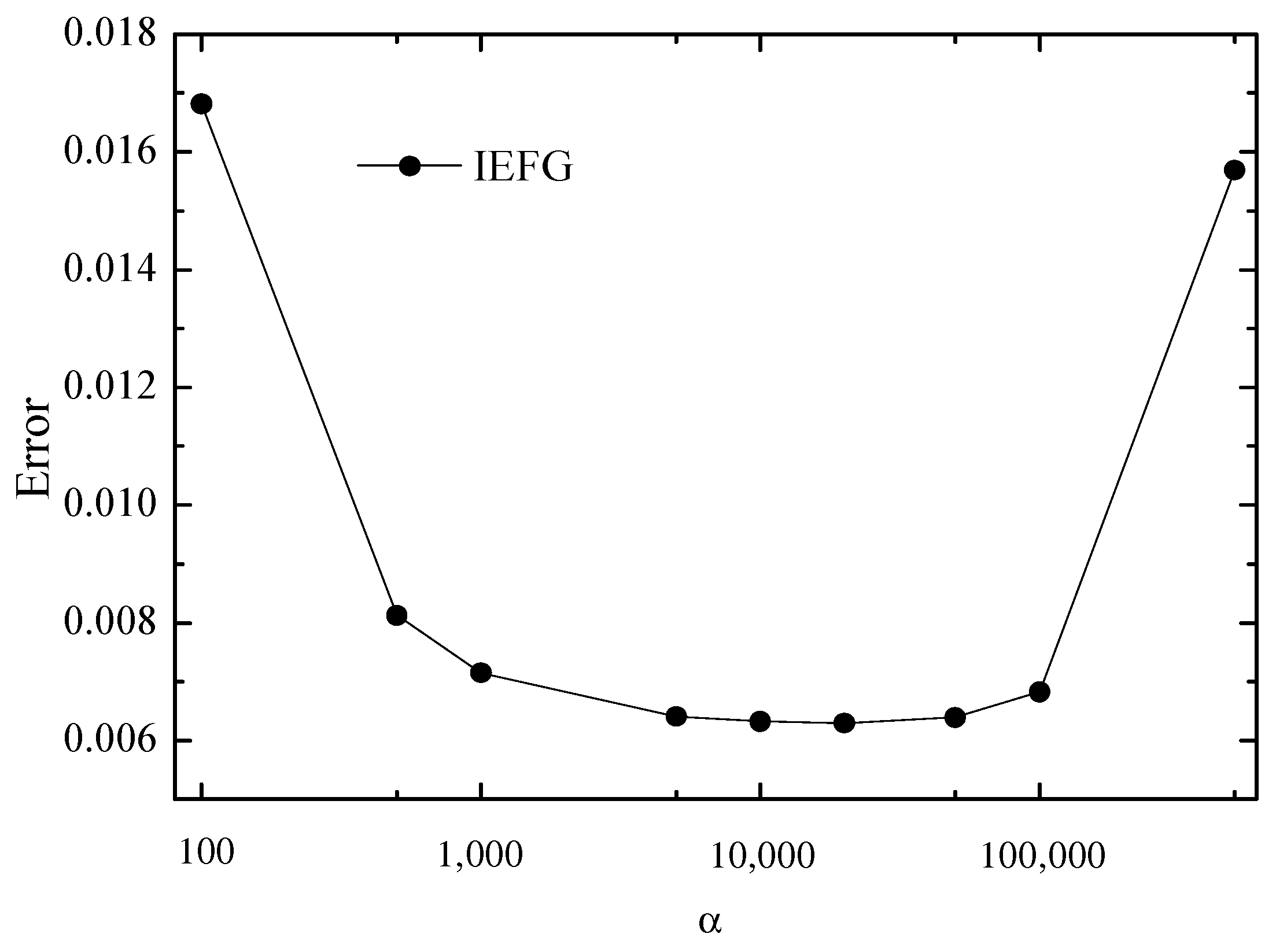
- Penalty factor
5. Conclusions
Author Contributions
Funding
Institutional Review Board Statement
Informed Consent Statement
Data Availability Statement
Conflicts of Interest
References
- Bouillarda, P.H.; Suleaub, S. Element-Free Galerkin solutions for Helmholtz problems: Formulation and numerical assessment of the pollution effect. Comput. Methods Appl. Mech. Eng. 1998, 162, 317–335. [Google Scholar] [CrossRef]
- Zeng, H.; Peng, L.; Zhao, G.; Han, C. A meshless Galerkin least-square method for the Helmholtz equation. Eng. Anal. Bound. Elem. 2011, 35, 868–878. [Google Scholar]
- Miao, Y.; Wang, Y.; Wang, Y.H. A meshless hybrid boundary-node method for Helmholtz problems. Eng. Anal. Bound. Elem. 2009, 33, 120–127. [Google Scholar] [CrossRef]
- Chen, L.C.; Liu, X.; Li, X.L. The boundary element-free method for 2D interior and exterior Helmholtz problems. Comput. Math. Appl. 2019, 77, 846–864. [Google Scholar]
- Li, X.L.; Zhang, S.G.; Wang, Y.; Chen, H. A complex variable boundary element-free method for potential and Helmholtz problems in three dimensions. Int. J. Comput. Methods 2020, 17, 1850129. [Google Scholar] [CrossRef]
- Chen, L.C.; Li, X.L. A complex variable boundary element-free method for the Helmholtz equation using regularized combined field integral equations. Appl. Math. Lett. 2020, 101, 106067. [Google Scholar] [CrossRef]
- Savovic, S.; Djordjevich, A. Numerical solution of diffusion equation describing the flow of radon through concrete. Appl. Radiat. Isot. 2008, 66, 552–555. [Google Scholar] [CrossRef] [PubMed]
- Ashyralyev, A.; Aggez, N. Finite Difference Method for Hyperbolic Equations with the Nonlocal Integral Condition. Discret. Dyn. Nat. Soc. 2011, 2011, 562385. [Google Scholar] [CrossRef] [Green Version]
- Ivanovic, M.; Svicevic, M.; Savovic, S. Numerical solution of Stefan problem with variable space grid method based on mixed finite element/finite difference approach. Int. J. Numer. Methods Heat Fluid Flow 2017, 27, 2682–2695. [Google Scholar] [CrossRef]
- Sowmiya, G.K.; Revathi, M. Numerical Method of Linear Hyperbolic Partial Differential Equation by Finite Difference Method with Conservation Law. Int. J. Adv. Sci. Technol. 2020, 29, 14–23. [Google Scholar]
- Thounthong, P.; Khan, M.N.; Hussain, I.; Ahmad, I.; Kumam, P. Symmetric radial basis function method for simulation of elliptic partial differential equations. Mathematics 2018, 6, 327. [Google Scholar] [CrossRef] [Green Version]
- Ahmad, I.; Ahsan, M.; Din, Z.U.; Ahmad, M.; Kumam, P. An efficient local formulation for time-dependent PDEs. Mathematics 2019, 7, 216. [Google Scholar] [CrossRef] [Green Version]
- Ahmad, I.; Ahmad, H.; Thounthong, P.; Chu, Y.M.; Cesarano, C. Solution of multi-term time-fractional PDE models arising in mathematical biology and physics by local meshless method. Symmetry 2020, 12, 1195. [Google Scholar] [CrossRef]
- Wang, F.Z.; Zheng, K.H.; Ahmad, I.; Ahmad, H. Gaussian radial basis functions method for linear and nonlinear convection-diffusion models in physical phenomen. Open Phys. 2021, 19, 69–76. [Google Scholar] [CrossRef]
- Dai, B.D.; Cheng, Y.M. Local boundary integral equation method based on radial basis functions for potential problems. Acta Phys. Sin. 2007, 56, 597–603. [Google Scholar]
- Belytschko, T.; Lu, Y.Y.; Gu, L. Element-free Galerkin Methods. Int. J. Numer. Methods Eng. 1994, 37, 229–256. [Google Scholar] [CrossRef]
- Cheng, R.J.; Cheng, Y.M. Error estimates of element-free Galerkin method for potential problems. Acta Phys. Sin. 2008, 57, 6037–6046. [Google Scholar]
- Cheng, J. Residential land leasing and price under public land ownership. J. Urban Plan. Dev. 2021, 147, 05021009. [Google Scholar] [CrossRef]
- Cheng, J. Analysis of commercial land leasing of the district governments of Beijing in China. Land Use Policy 2021, 100, 104881. [Google Scholar] [CrossRef]
- Cheng, J. Analyzing the factors influencing the choice of the government on leasing different types of land uses: Evidence from Shanghai of China. Land Use Policy 2020, 90, 104303. [Google Scholar] [CrossRef]
- Cheng, J. Data analysis of the factors influencing the industrial land leasing in Shanghai based on mathematical models. Math. Probl. Eng. 2020, 2020, 9346863. [Google Scholar] [CrossRef] [Green Version]
- Cheng, J. Mathematical models and data analysis of residential land leasing behavior of district governments of Beijing in China. Mathematics 2021, 9, 2314. [Google Scholar] [CrossRef]
- Cheng, Y.M.; Chen, M.J. A boundary element-free method for linear elasticity. Acta Mech. Sin. 2003, 35, 181–186. [Google Scholar]
- Zhang, Z.; Zhao, P.; Liew, K.M. Analyzing three-dimensional potential problems with the improved element-free Galerkin method. Comput. Mech. 2009, 44, 273–284. [Google Scholar] [CrossRef]
- Zhang, Z.; Wang, J.F.; Cheng, Y.M.; Liew, K.M. The improved element-free Galerkin method for three-dimensional transient heat conduction problems. Sci. China Phys. Mech. Astron. 2013, 56, 1568–1580. [Google Scholar] [CrossRef]
- Zhang, Z.; Li, D.M.; Cheng, Y.M.; Liew, K.M. The improved element-free Galerkin method for three-dimensional wave equation. Acta Mech. Sin. 2012, 28, 808–818. [Google Scholar] [CrossRef]
- Cheng, R.J.; Cheng, Y.M. Solving unsteady Schrödinger equation using the improved element-free Galerkin method. Chin. Phys. B 2016, 25, 020203. [Google Scholar] [CrossRef]
- Cheng, H.; Zheng, G.D. Analyzing 3D advection-diffusion problems by using the improved element-free Galerkin method. Math. Probl. Eng. 2020, 2020, 4317538. [Google Scholar] [CrossRef]
- Zhang, Z.; Hao, S.Y.; Liew, K.M.; Cheng, Y.M. The improved element-free Galerkin method for two-dimensional elastodynamics problems. Eng. Anal. Bound. Elem. 2013, 37, 1576–1584. [Google Scholar] [CrossRef]
- Yu, S.Y.; Peng, M.J.; Cheng, H.; Cheng, Y.M. The improved element-free Galerkin method for three-dimensional elastoplasticity problems. Eng. Anal. Bound. Elem. 2019, 104, 215–224. [Google Scholar] [CrossRef]
- Peng, M.J.; Li, R.X.; Cheng, Y.M. Analyzing three-dimensional viscoelasticity problems via the improved element-free Galerkin (IEFG) method. Eng. Anal. Bound. Elem. 2014, 40, 104–113. [Google Scholar] [CrossRef]
- Zheng, G.D.; Cheng, Y.M. The improved element-free Galerkin method for diffusional drug release problems. Int. J. Appl. Mech. 2020, 12, 2050096. [Google Scholar] [CrossRef]
- Zhang, Z.; Liew, K.M.; Cheng, Y.M.; Lee, Y.Y. Analyzing 2D fracture problems with the improved element-free Galerkin method. Eng. Anal. Bound. Elem. 2008, 32, 241–250. [Google Scholar] [CrossRef]
- Cai, X.J.; Peng, M.J.; Cheng, Y.M. The improved element-free Galerkin method for elastoplasticity large deformation problems. Sci. Sin. Phys. Mech. Astron. 2018, 48, 024701. [Google Scholar] [CrossRef]
- Lancaster, P.; Salkauskas, K. Surfaces generated by moving least squares methods. Math. Comput. 1981, 37, 141–158. [Google Scholar] [CrossRef]
- Ren, H.P.; Cheng, Y.M.; Zhang, W. Researches on the improved interpolating moving least-squares method. Chin. J. Eng. Math. 2010, 27, 1021–1029. [Google Scholar]
- Ren, H.P.; Cheng, Y.M. The interpolating element-free Galerkin (IEFG) method for two-dimensional potential problems. Eng. Anal. Bound. Elem. 2012, 36, 873–880. [Google Scholar] [CrossRef]
- Liu, D.; Cheng, Y.M. The interpolating element-free Galerkin method for three-dimensional transient heat conduction problems. Results Phys. 2020, 19, 103477. [Google Scholar] [CrossRef]
- Wu, Q.; Liu, F.B.; Cheng, Y.M. The interpolating element-free Galerkin method for three-dimensional elastoplasticity problems. Eng. Anal. Bound. Elem. 2020, 115, 156–167. [Google Scholar] [CrossRef]
- Wu, Q.; Peng, P.P.; Cheng, Y.M. The interpolating element-free Galerkin method for elastic large deformation problems. Sci. China Technol. Sci. 2021, 64, 364–374. [Google Scholar] [CrossRef]
- Cheng, Y.M.; Bai, F.N.; Liu, C.; Peng, M.J. Analyzing nonlinear large deformation with an improved element-free Galerkin method via the interpolating moving least-squares method. Int. J. Comput. Mater. Sci. Eng. 2016, 5, 1650023. [Google Scholar]
- Qin, Y.X.; Li, Q.Y.; Du, H.X. Interpolating smoothed particle method for elastic axisymmetrical problem. Int. J. Appl. Mech. 2017, 9, 1750022. [Google Scholar] [CrossRef]
- Wang, J.F.; Sun, F.X.; Cheng, Y.M. An improved interpolating element-free Galerkin method with nonsingular weight function for two-dimensional potential problems. Chin. Phys. B 2012, 21, 090204. [Google Scholar] [CrossRef]
- Liu, F.B.; Cheng, Y.M. The improved element-free Galerkin method based on the nonsingular weight functions for elastic large deformation problems. Int. J. Comput. Mater. Sci. Eng. 2018, 7, 1850023. [Google Scholar] [CrossRef]
- Liu, F.B.; Wu, Q.; Cheng, Y.M. A meshless method based on the nonsingular weight functions for elastoplastic large deformation problems. Int. J. Appl. Mech. 2019, 11, 1950006. [Google Scholar] [CrossRef]
- Liu, F.B.; Cheng, Y.M. The improved element-free Galerkin method based on the nonsingular weight functions for inhomogeneous swelling of polymer gels. Int. J. Appl. Mech. 2018, 10, 1850047. [Google Scholar] [CrossRef]
- Cheng, Y.M.; Peng, M.J.; Li, J.H. The complex variable moving least-square approximation and its application. Acta Mech. Sin. 2005, 37, 719–723. [Google Scholar]
- Peng, M.J.; Liu, P.; Cheng, Y.M. The complex variable element-free Galerkin (CVEFG) method for two-dimensional elasticity problems. Int. J. Appl. Mech. 2009, 1, 367–385. [Google Scholar] [CrossRef]
- Bai, F.N.; Li, D.M.; Wang, J.F.; Cheng, Y.M. An improved complex variable element-free Galerkin method for two-dimensional elasticity problems. Chin. Phys. B 2012, 21, 020204. [Google Scholar] [CrossRef]
- Chen, L.; Cheng, Y.M. Reproducing kernel particle method with complex variables for elasticity. Acta Phys. Sin. 2008, 57, 1–10. [Google Scholar] [CrossRef]
- Chen, L.; Cheng, Y.M. The complex variable reproducing kernel particle method for elasto-plasticity problems. Sci. China Phys. Mech. Astron. 2010, 53, 954–965. [Google Scholar] [CrossRef]
- Cheng, H.; Peng, M.J.; Cheng, Y.M. The dimension splitting and improved complex variable element-free Galerkin method for 3-dimensional transient heat conduction problems. Int. J. Numer. Methods Eng. 2018, 114, 321–345. [Google Scholar] [CrossRef]
- Cheng, H.; Peng, M.J.; Cheng, Y.M. A hybrid improved complex variable element-free Galerkin method for three-dimensional potential problems. Eng. Anal. Bound. Elem. 2017, 84, 52–62. [Google Scholar] [CrossRef]
- Cheng, H.; Peng, M.J.; Cheng, Y.M. A fast complex variable element-free Galerkin method for three-dimensional wave propagation problems. Int. J. Appl. Mech. 2017, 9, 1750090. [Google Scholar] [CrossRef]
- Cheng, H.; Peng, M.J.; Cheng, Y.M. A hybrid improved complex variable element-free Galerkin method for three-dimensional advection-diffusion problems. Eng. Anal. Bound. Elem. 2018, 97, 39–54. [Google Scholar] [CrossRef]
- Cheng, H.; Peng, M.J.; Cheng, Y.M.; Meng, Z.J. The hybrid complex variable element-free Galerkin method for 3D elasticity problems. Eng. Struct. 2020, 219, 110835. [Google Scholar] [CrossRef]
- Meng, Z.J.; Cheng, H.; Ma, L.D.; Cheng, Y.M. The dimension split element-free Galerkin method for three-dimensional potential problems. Acta Mech. Sin. 2018, 34, 462–474. [Google Scholar] [CrossRef]
- Meng, Z.J.; Cheng, H.; Ma, L.D.; Cheng, Y.M. The dimension splitting element-free Galerkin method for 3D transient heat conduction problems. Sci. China Phys. Mech. Astron. 2019, 62, 040711. [Google Scholar] [CrossRef]
- Meng, Z.J.; Cheng, H.; Ma, L.D.; Cheng, Y.M. The hybrid element-free Galerkin method for three-dimensional wave propagation problems. Int. J. Numer. Methods Eng. 2019, 117, 15–37. [Google Scholar] [CrossRef] [Green Version]
- Ma, L.D.; Meng, Z.J.; Chai, J.F.; Cheng, Y.M. Analyzing 3D advection-diffusion problems by using the dimension splitting element-free Galerkin method. Eng. Anal. Bound. Elem. 2020, 111, 167–177. [Google Scholar] [CrossRef]
- Peng, P.P.; Wu, Q.; Cheng, Y.M. The dimension splitting reproducing kernel particle method for three-dimensional potential problems. Int. J. Numer. Methods Eng. 2020, 121, 146–164. [Google Scholar] [CrossRef]
- Peng, P.P.; Cheng, Y.M. Analyzing three-dimensional transient heat conduction problems with the dimension splitting reproducing kernel particle method. Eng. Anal. Bound. Elem. 2020, 121, 180–191. [Google Scholar] [CrossRef]
- Peng, P.P.; Cheng, Y.M. Analyzing three-dimensional wave propagation with the hybrid reproducing kernel particle method based on the dimension splitting method. Eng. Comput. 2021, 1–17. [Google Scholar] [CrossRef]
- Peng, P.P.; Cheng, Y.M. A hybrid reproducing kernel particle method for three-dimensional advection-diffusion problems. Int. J. Appl. Mech. 2021, 13, 2150085. [Google Scholar] [CrossRef]
- Wu, Q.; Peng, M.J.; Cheng, Y.M. The interpolating dimension splitting element-free Galerkin method for 3D potential problems. Eng. Comput. 2021, 1–15. [Google Scholar] [CrossRef]
- Wang, J.F.; Sun, F.X. A hybrid generalized interpolated element-free Galerkin method for Stokes problems. Eng. Anal. Bound. Elem. 2020, 111, 88–100. [Google Scholar] [CrossRef]
- Marin, L. A meshless method for the numerical solution of the Cauchy problem associated with three-dimensional Helmholtz-type equations. Appl. Math. Comput. 2005, 165, 274–355. [Google Scholar] [CrossRef]
- Cheng, D.S.; Chen, B.W.; Chen, X.L. A robust optimal finite difference scheme for the three-dimensional Helmholtz equation. Math. Probl. Eng. 2019, 2019, 8532408. [Google Scholar] [CrossRef] [Green Version]


| Nodes | Relative Error | Time (s) | ||
|---|---|---|---|---|
| IEFG | EFG | IEFG | EFG | |
| 7 × 7 × 7 | 4.3092% | 4.3092% | 5.5 | 5.8 |
| 11 × 11 × 11 | 1.3234% | 1.3234% | 26.7 | 28.5 |
| 13 × 13 × 13 | 0.8832% | 0.8832% | 49.9 | 53.1 |
| 15 × 15 × 15 | 0.6296% | 0.6296% | 92.1 | 98.0 |
| 17 × 17 × 17 | 0.4706% | 0.4706% | 152.0 | 161.9 |
| 21 × 21 × 21 | 0.2905% | 0.2905% | 384.5 | 398.6 |
| 25 × 25 × 25 | 0.1967% | 0.1967% | 903.3 | 940.2 |
| 29 × 29 × 29 | 0.1520% | 0.1520% | 1907.2 | 1937.1 |
| 33 × 33 × 33 | 0.1075% | 0.1075% | 4287.2 | 4408.3 |
Publisher’s Note: MDPI stays neutral with regard to jurisdictional claims in published maps and institutional affiliations. |
© 2021 by the authors. Licensee MDPI, Basel, Switzerland. This article is an open access article distributed under the terms and conditions of the Creative Commons Attribution (CC BY) license (https://creativecommons.org/licenses/by/4.0/).
Share and Cite
Cheng, H.; Peng, M. The Improved Element-Free Galerkin Method for 3D Helmholtz Equations. Mathematics 2022, 10, 14. https://doi.org/10.3390/math10010014
Cheng H, Peng M. The Improved Element-Free Galerkin Method for 3D Helmholtz Equations. Mathematics. 2022; 10(1):14. https://doi.org/10.3390/math10010014
Chicago/Turabian StyleCheng, Heng, and Miaojuan Peng. 2022. "The Improved Element-Free Galerkin Method for 3D Helmholtz Equations" Mathematics 10, no. 1: 14. https://doi.org/10.3390/math10010014
APA StyleCheng, H., & Peng, M. (2022). The Improved Element-Free Galerkin Method for 3D Helmholtz Equations. Mathematics, 10(1), 14. https://doi.org/10.3390/math10010014