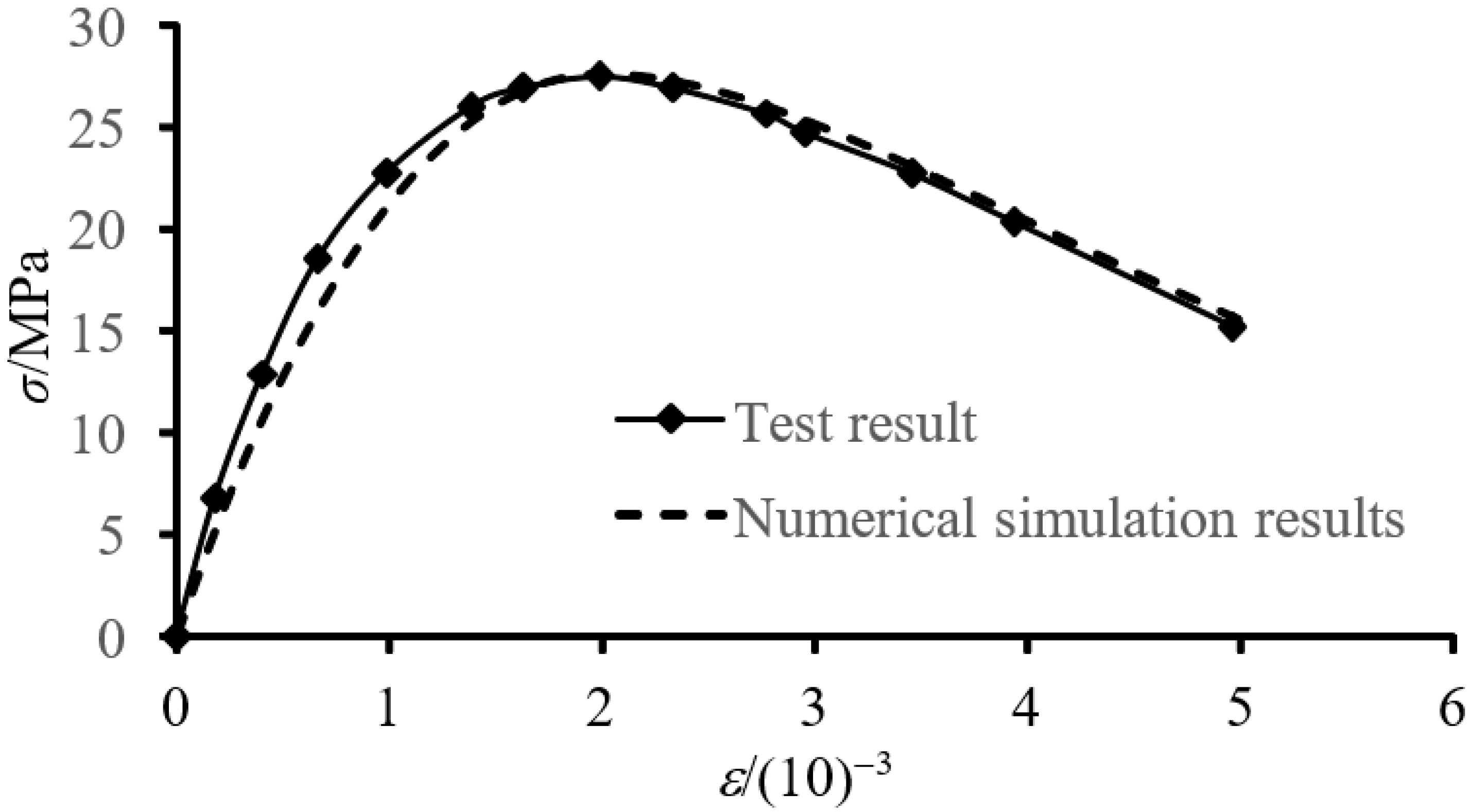
Figure 1.
Comparison of numerical simulation result and experimental result (uniaxial tensile test).
Figure 1.
Comparison of numerical simulation result and experimental result (uniaxial tensile test).
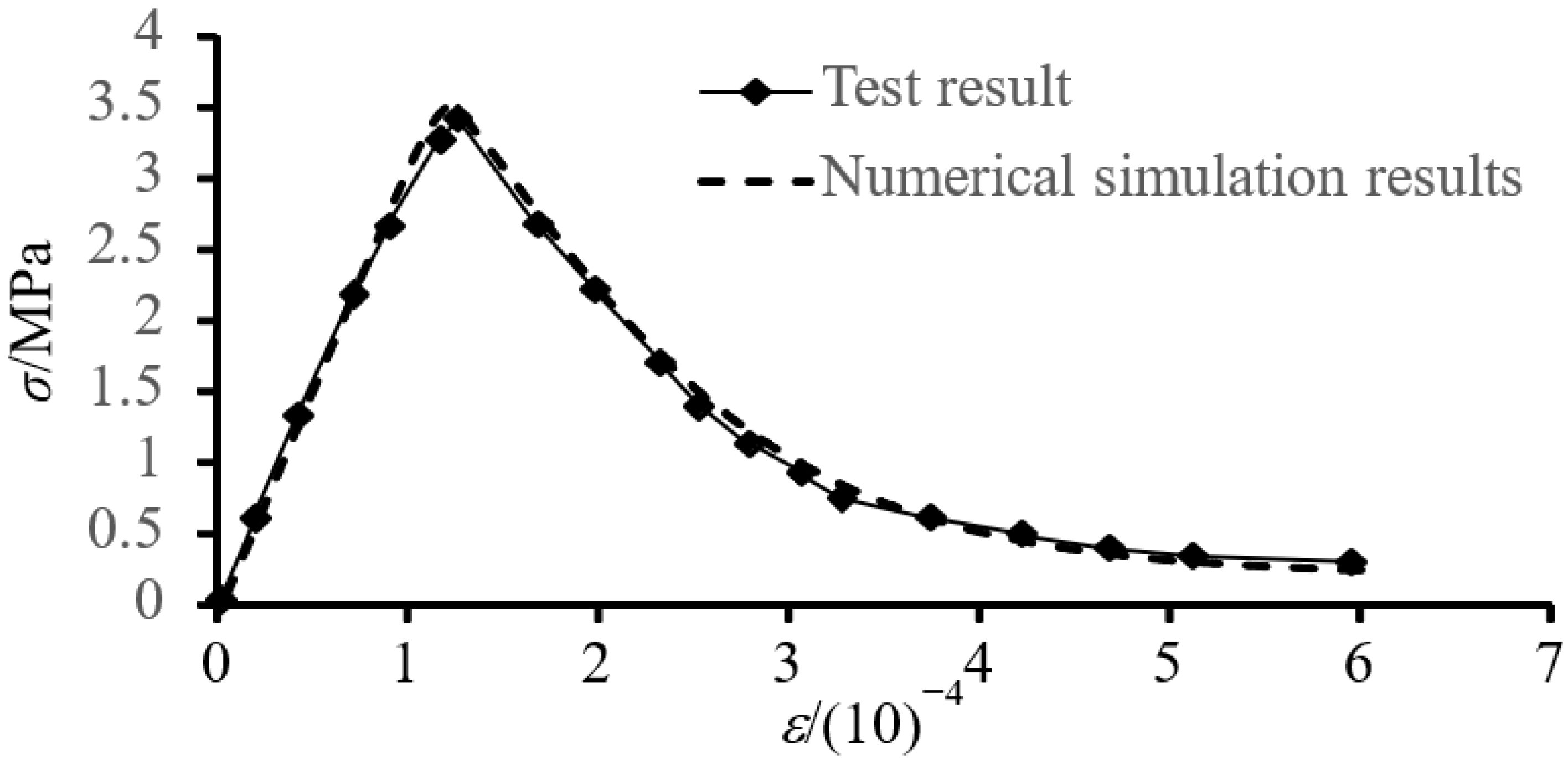
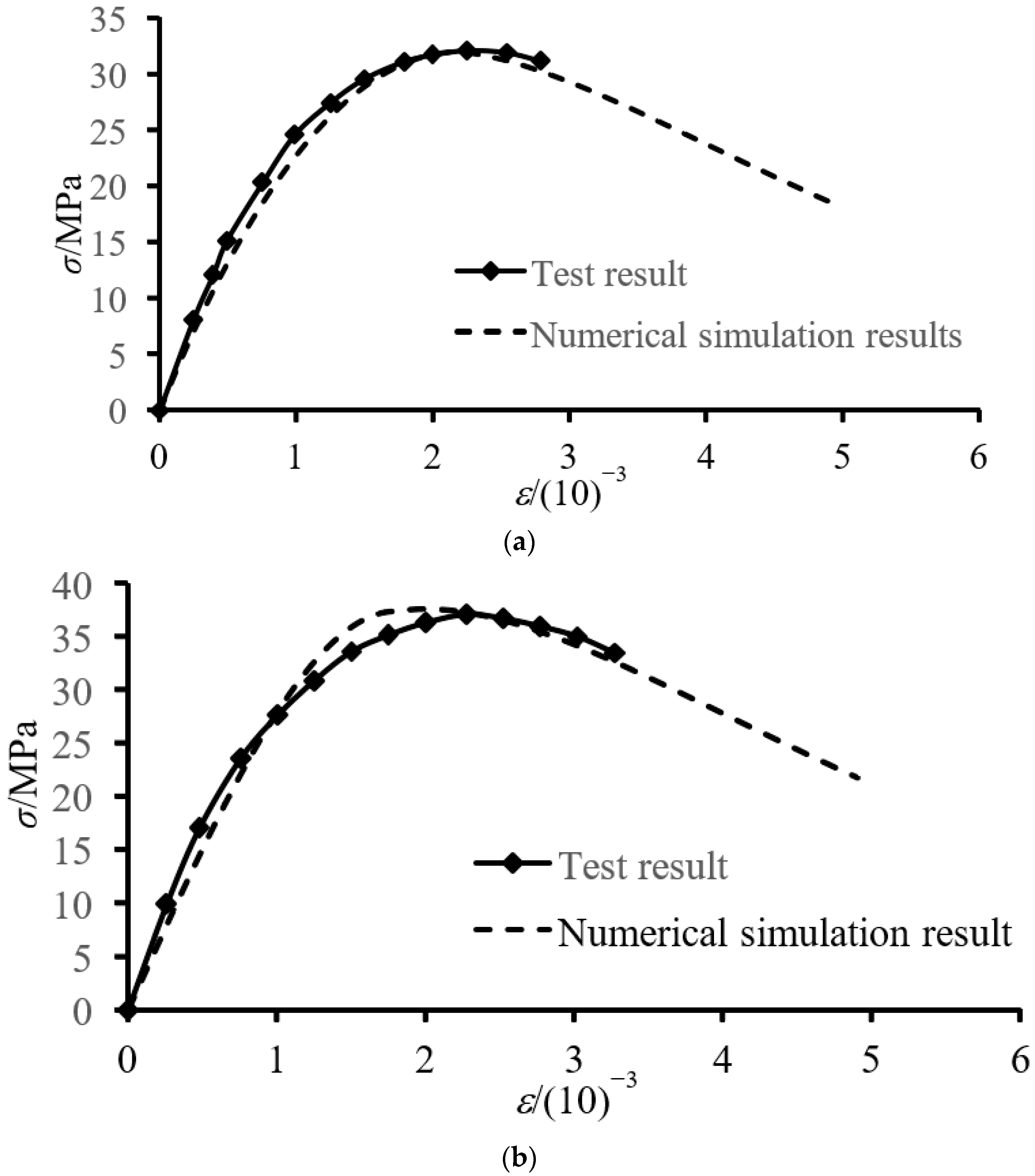
Figure 2.
Comparison of numerical simulation result and experimental result (uniaxial compression test).
Figure 2.
Comparison of numerical simulation result and experimental result (uniaxial compression test).
Figure 3.
Comparison of numerical simulation result and experimental result (biaxial stress test). (a) σ1/σ2= −1:0; (b) σ1/σ2= −1:−1.
Figure 3.
Comparison of numerical simulation result and experimental result (biaxial stress test). (a) σ1/σ2= −1:0; (b) σ1/σ2= −1:−1.
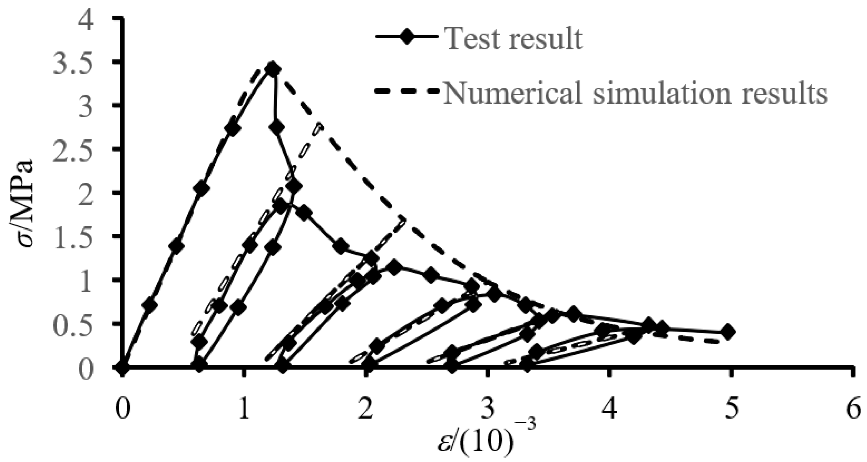
Figure 4.
Comparison of numerical simulation result and experimental result (cyclic tensile test).
Figure 4.
Comparison of numerical simulation result and experimental result (cyclic tensile test).
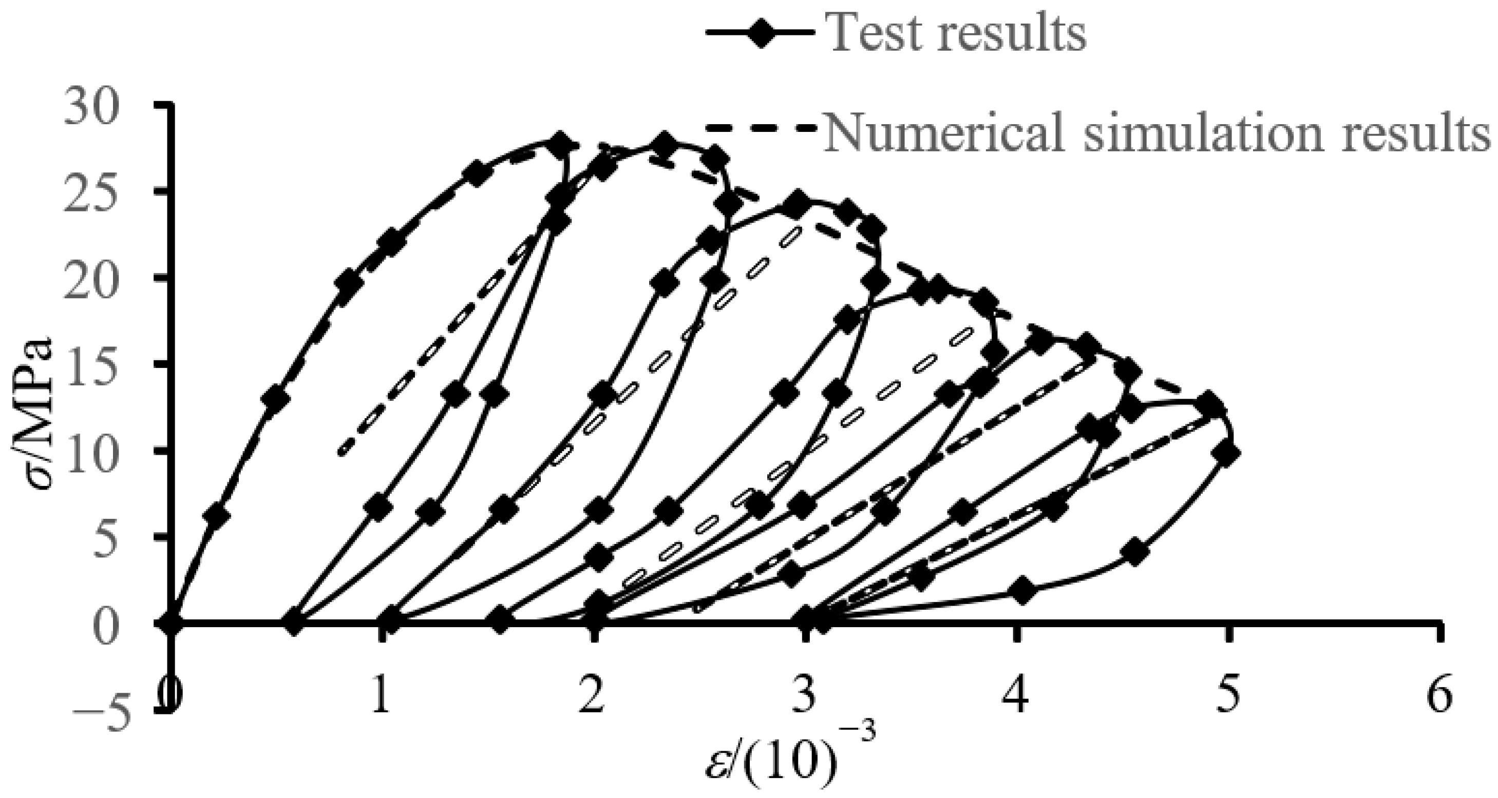
Figure 5.
Comparison of numerical simulation result and experimental result (cyclic compression test).
Figure 5.
Comparison of numerical simulation result and experimental result (cyclic compression test).
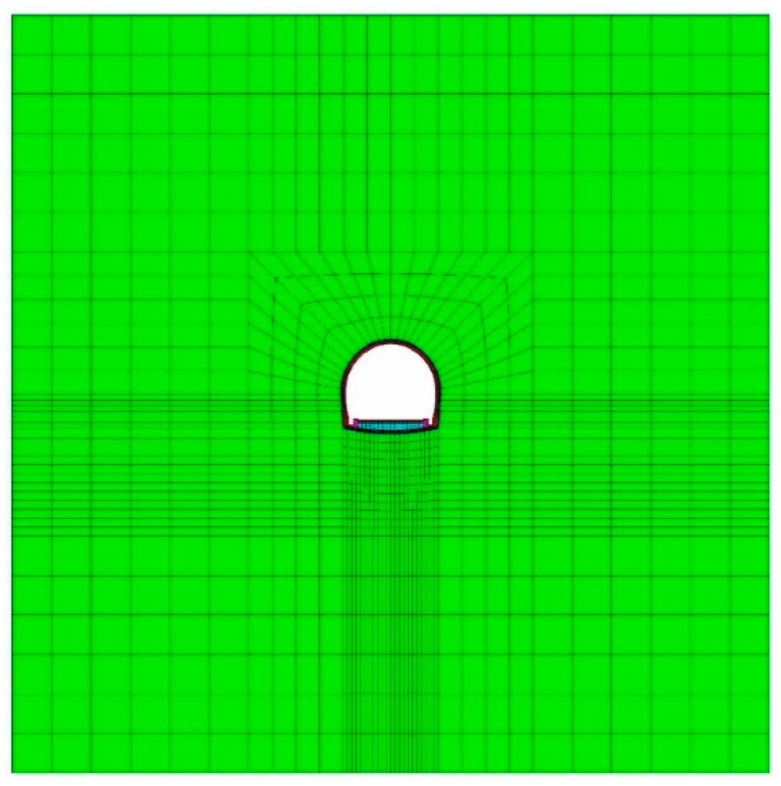
Figure 6.
Numerical simulation model.
Figure 6.
Numerical simulation model.
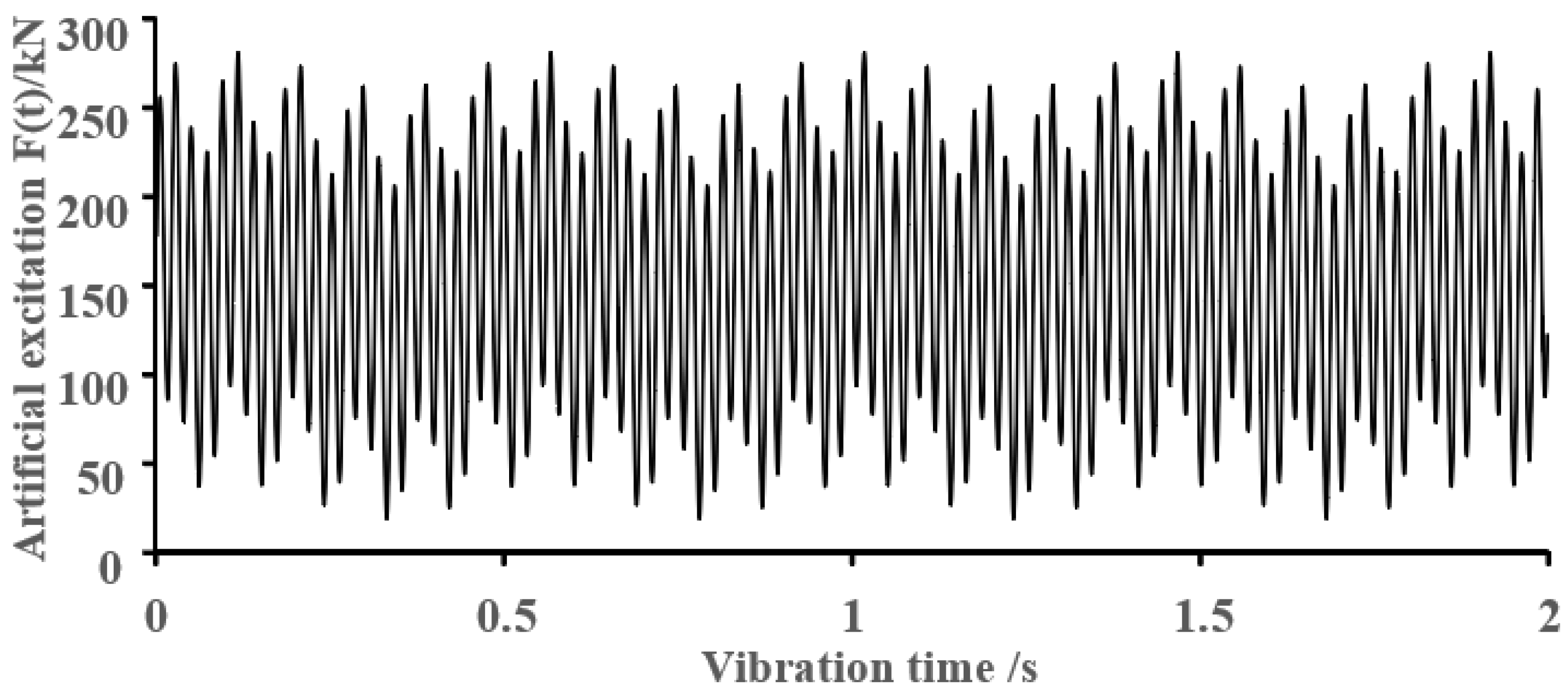
Figure 7.
Simulative train load time history curve.
Figure 7.
Simulative train load time history curve.
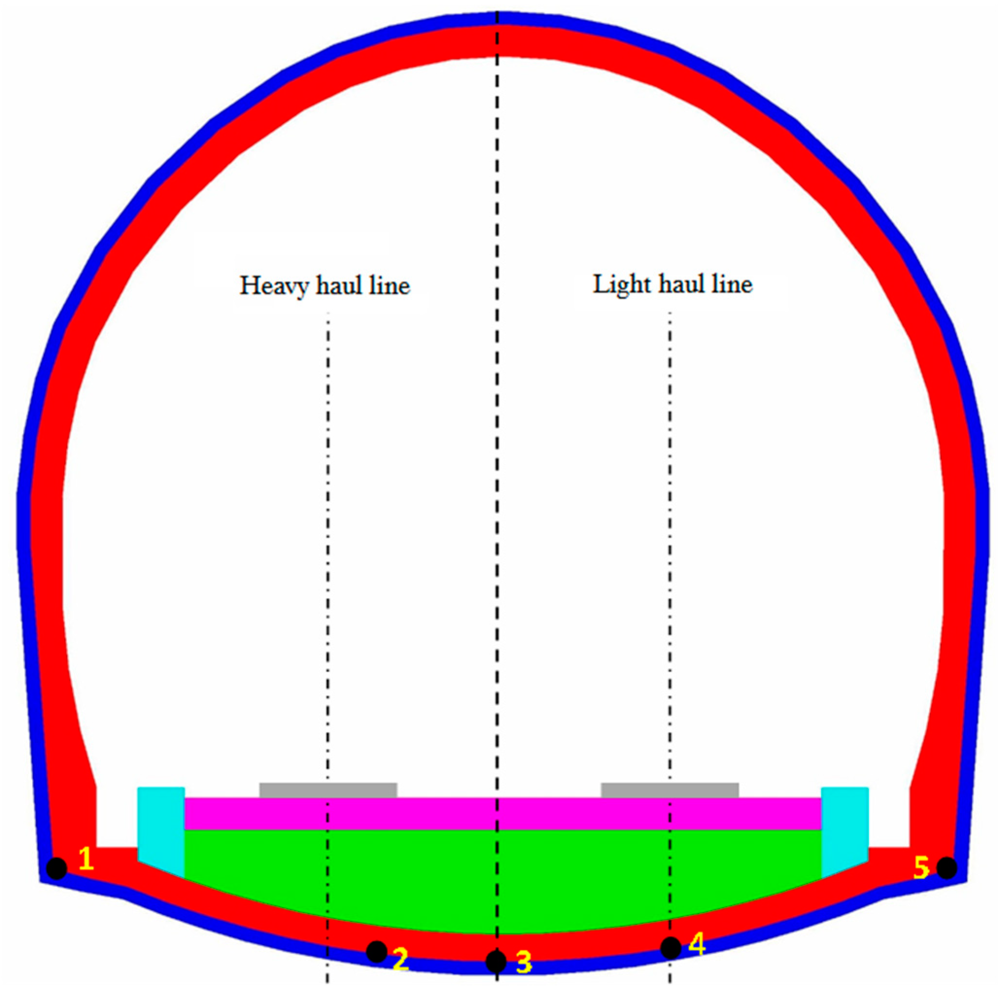
Figure 8.
Measuring point layout.
Figure 8.
Measuring point layout.
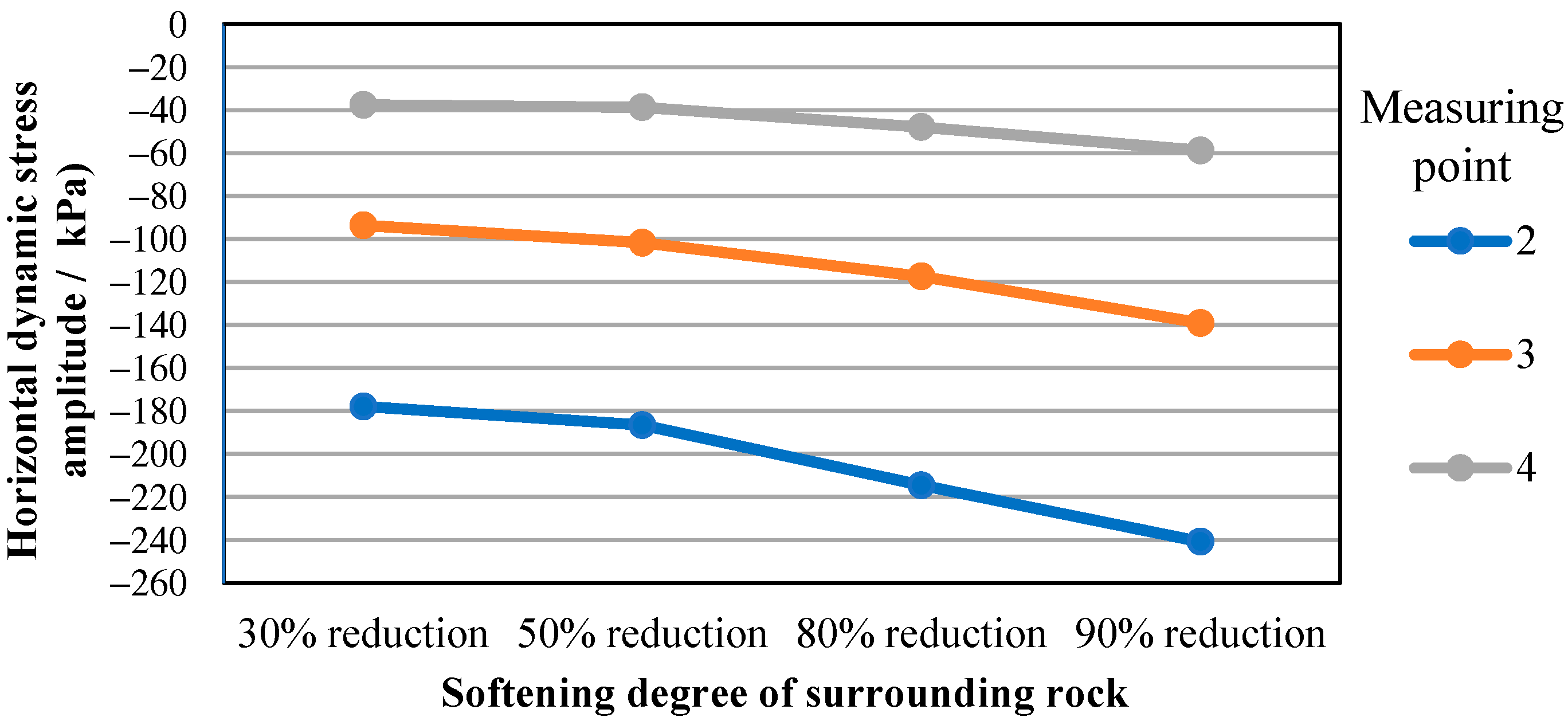
Figure 9.
Horizontal dynamic stress amplitudes of measuring points 2, 3, and 4 under different softening degrees of the basement surrounding rock.
Figure 9.
Horizontal dynamic stress amplitudes of measuring points 2, 3, and 4 under different softening degrees of the basement surrounding rock.
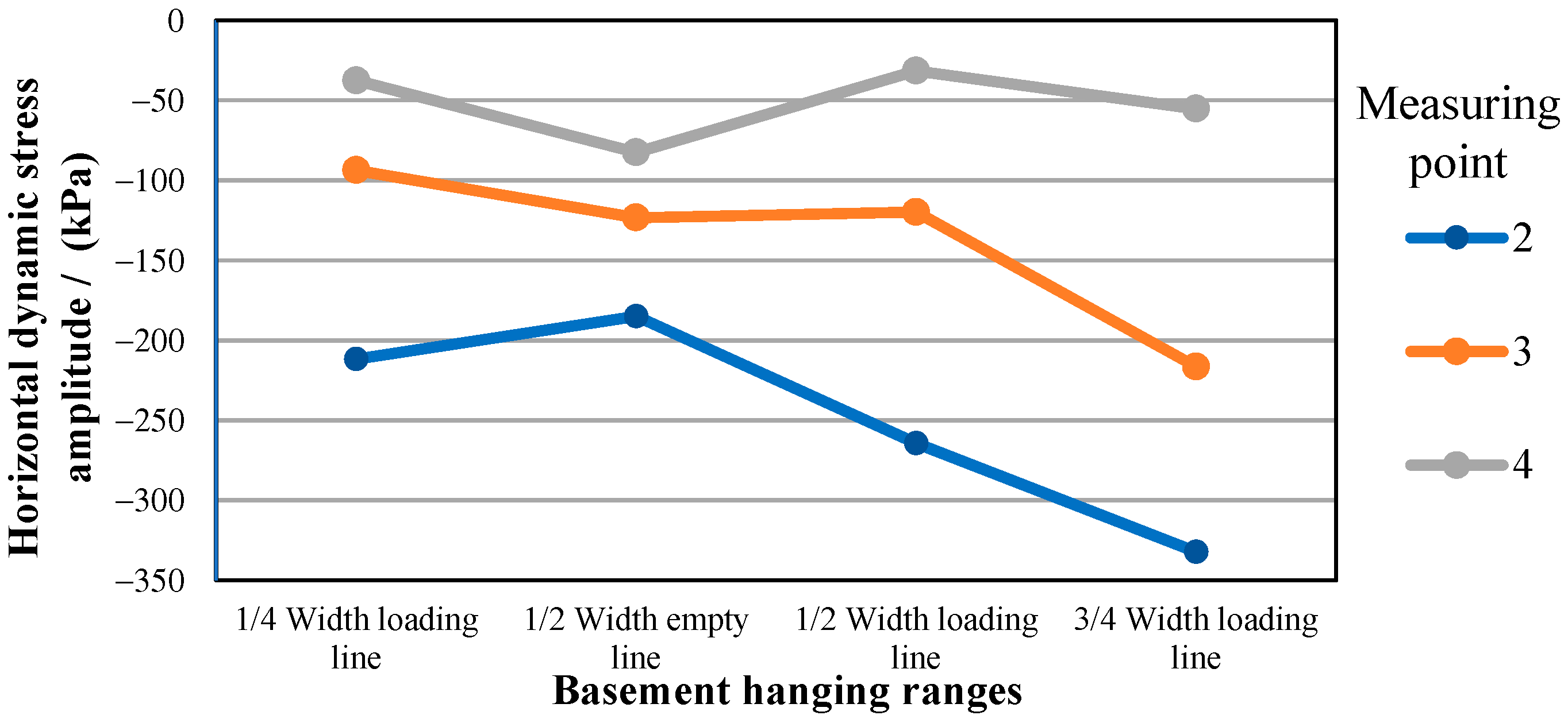
Figure 10.
Horizontal dynamic stress amplitudes diagram of measuring points 2, 3, and 4 under different basement hanging ranges.
Figure 10.
Horizontal dynamic stress amplitudes diagram of measuring points 2, 3, and 4 under different basement hanging ranges.
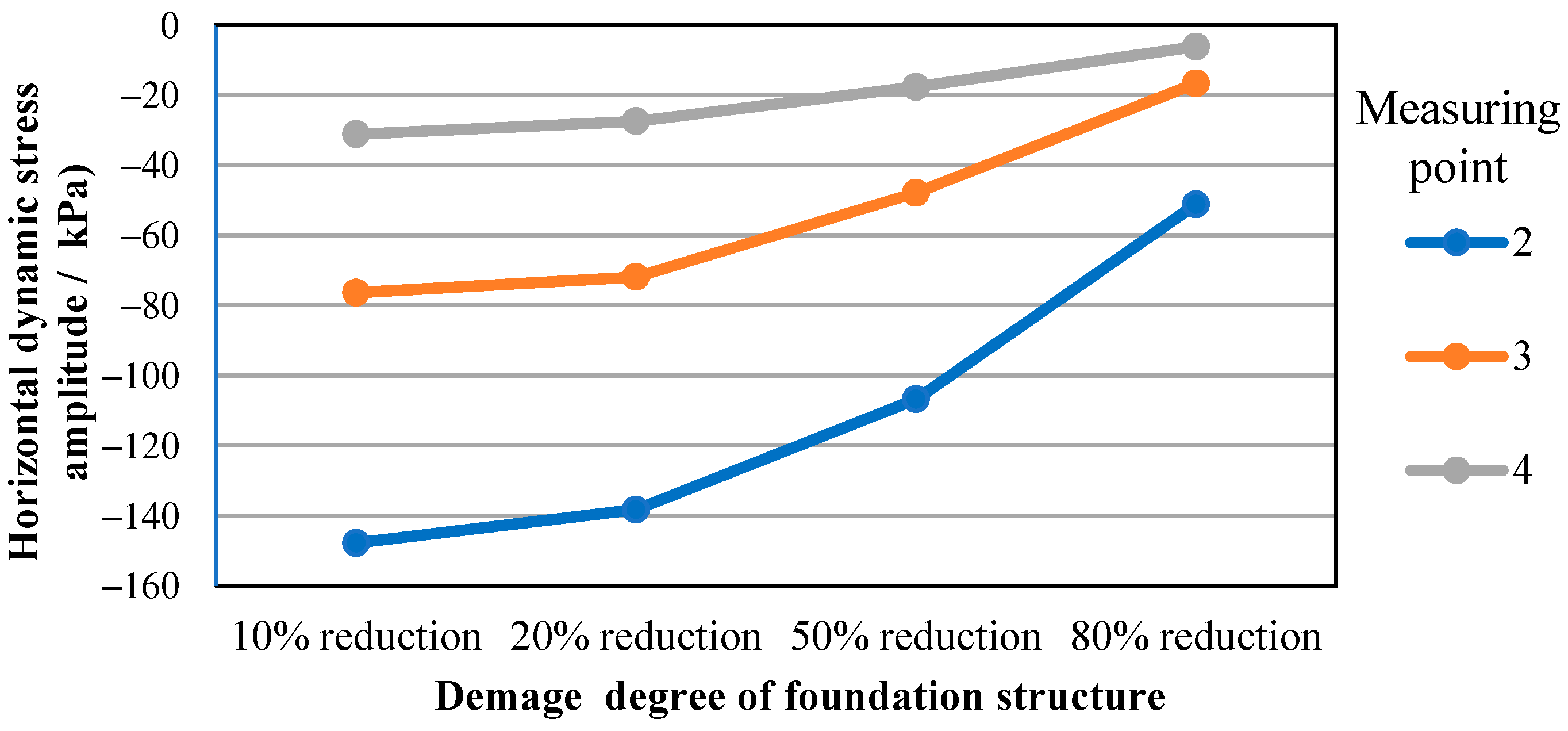
Figure 11.
Horizontal dynamic stress amplitudes diagram of measuring points 2, 3, and 4 under different degrees of damage to the foundation structure.
Figure 11.
Horizontal dynamic stress amplitudes diagram of measuring points 2, 3, and 4 under different degrees of damage to the foundation structure.
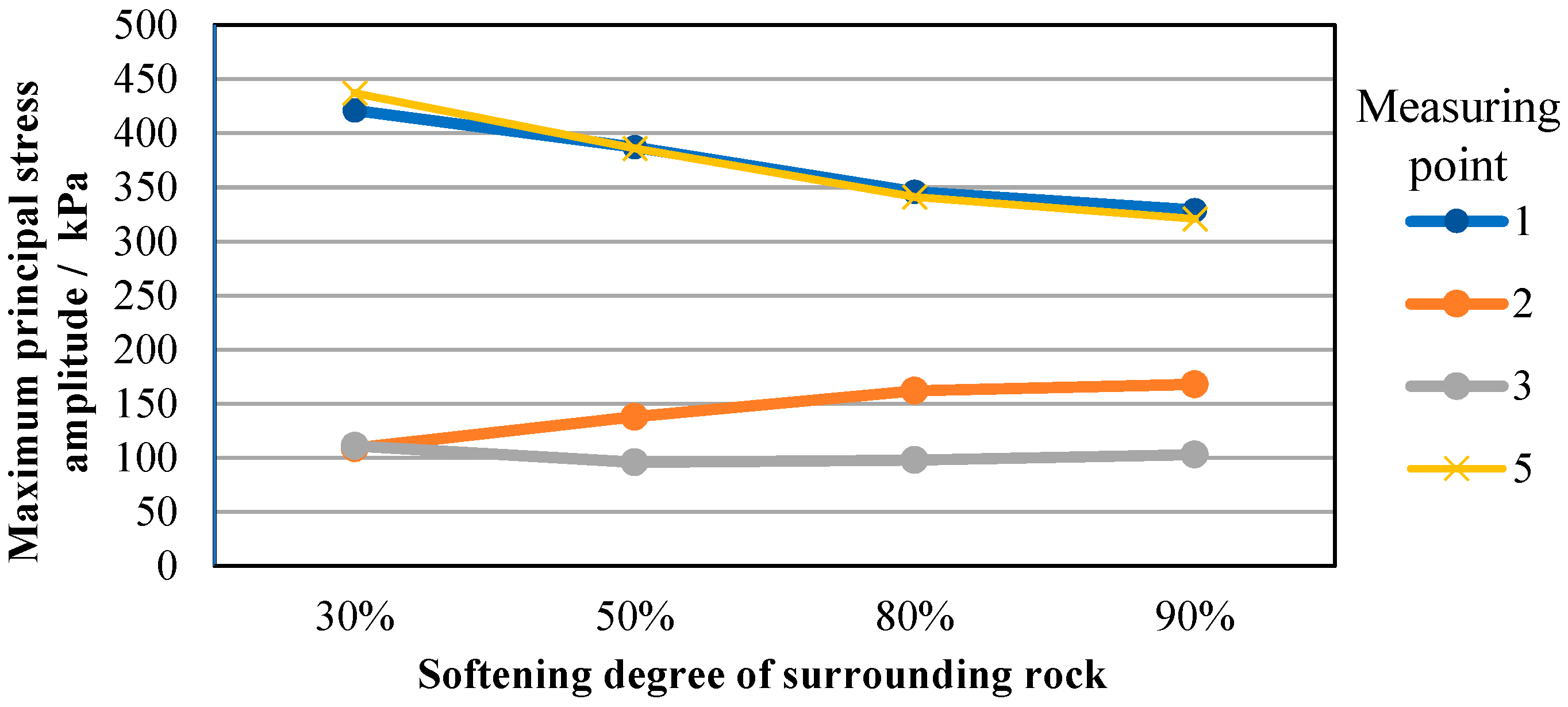
Figure 12.
Maximum principal stress amplitude diagram of measuring points 1, 2, 3, and 5 under different softening degrees of basement surrounding rock.
Figure 12.
Maximum principal stress amplitude diagram of measuring points 1, 2, 3, and 5 under different softening degrees of basement surrounding rock.
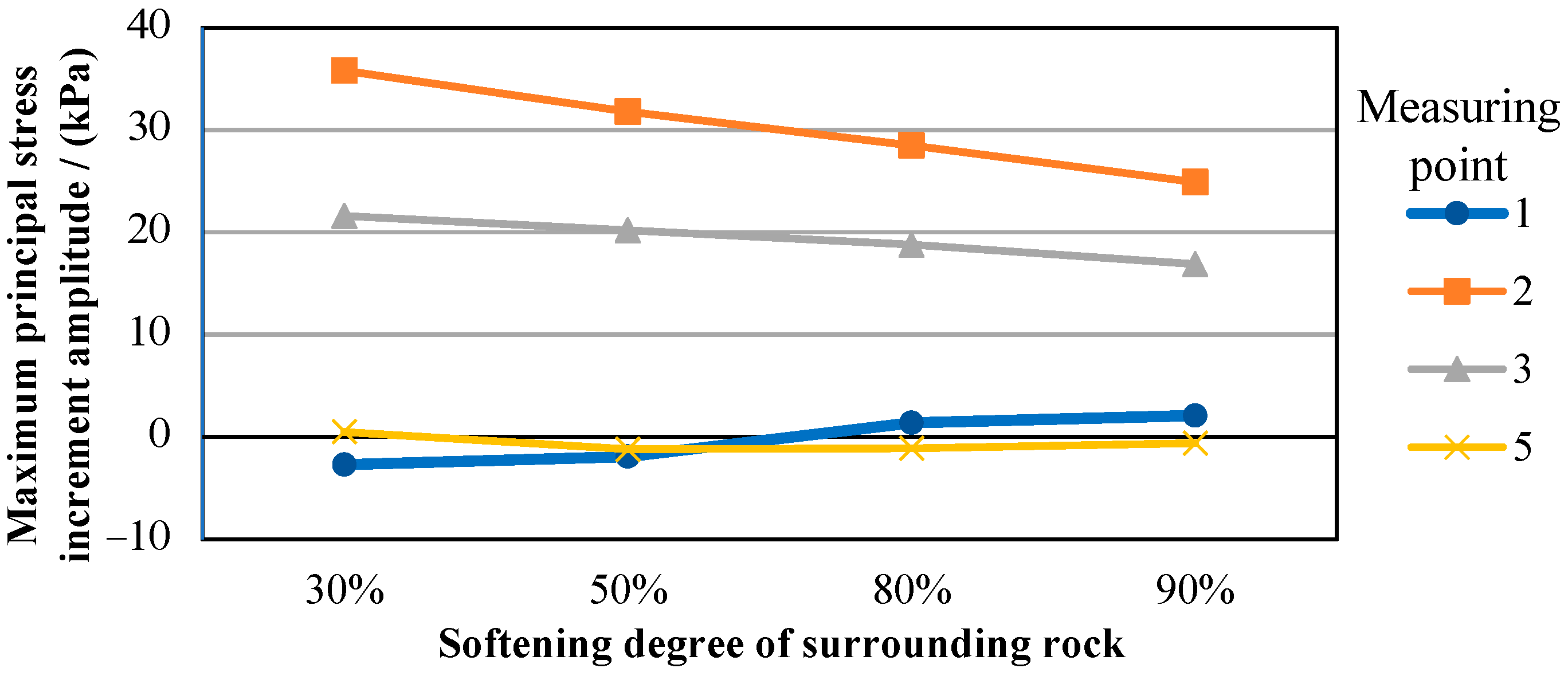
Figure 13.
Maximum principal stress increment amplitude of measuring points 1, 2, 3, and 5 under different softening degrees of basement surrounding rock.
Figure 13.
Maximum principal stress increment amplitude of measuring points 1, 2, 3, and 5 under different softening degrees of basement surrounding rock.
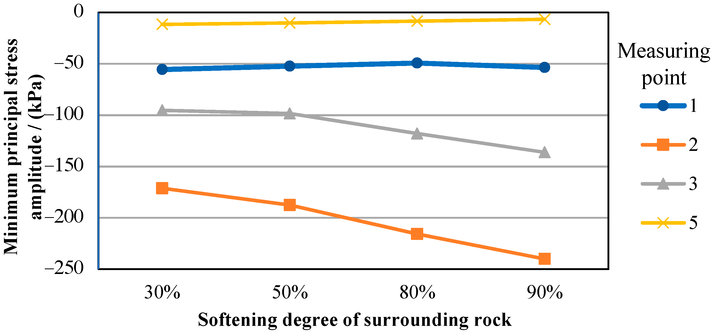
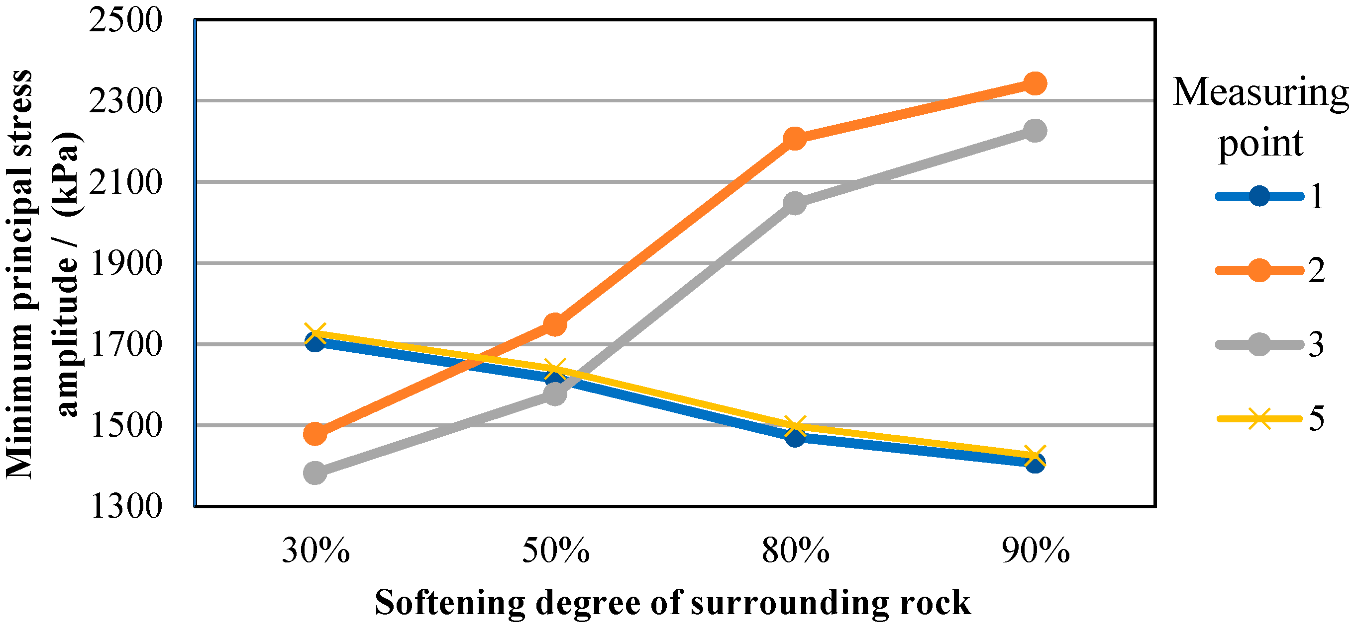
Figure 14.
Minimum principal stress amplitude diagram of measuring points 1, 2, 3, and 5 under different softening degrees of basement surrounding rock.
Figure 14.
Minimum principal stress amplitude diagram of measuring points 1, 2, 3, and 5 under different softening degrees of basement surrounding rock.
Figure 15.
Minimum principal stress increment amplitude diagram of measuring points 1, 2, 3, and 5 under different softening degrees of basement surrounding rock.
Figure 15.
Minimum principal stress increment amplitude diagram of measuring points 1, 2, 3, and 5 under different softening degrees of basement surrounding rock.
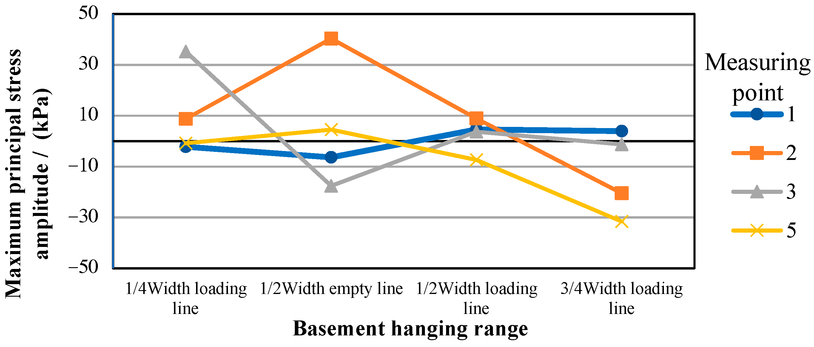
Figure 16.
Maximum principal stress increment amplitude diagram of measuring points 1, 2, 3, and 5 under different basement hanging ranges.
Figure 16.
Maximum principal stress increment amplitude diagram of measuring points 1, 2, 3, and 5 under different basement hanging ranges.
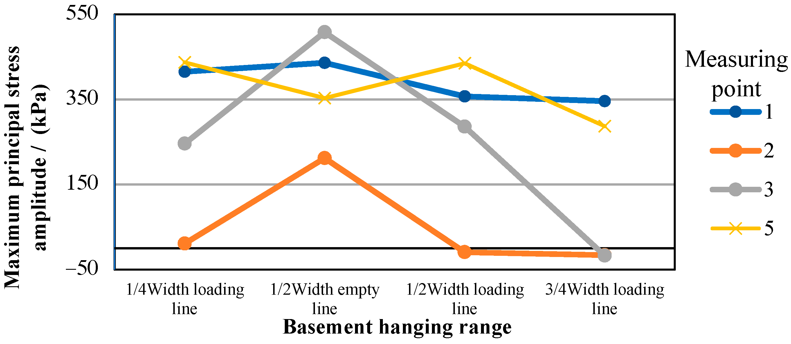
Figure 17.
Maximum principal stress amplitude diagram of measuring points 1, 2, 3, and 5 under different basement hanging ranges.
Figure 17.
Maximum principal stress amplitude diagram of measuring points 1, 2, 3, and 5 under different basement hanging ranges.
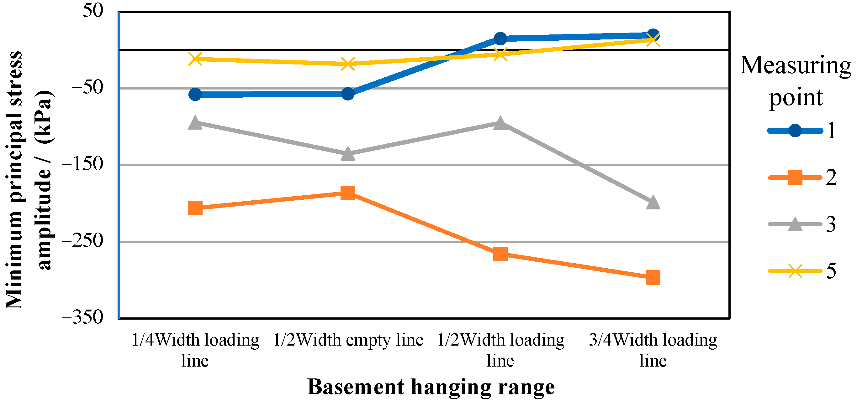
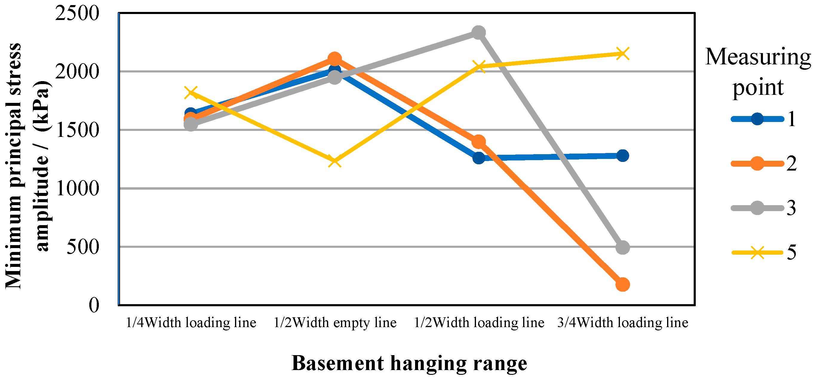
Figure 18.
Minimum principal stress amplitude diagram of measuring points 1, 2, 3, and 5 under different basement hanging ranges.
Figure 18.
Minimum principal stress amplitude diagram of measuring points 1, 2, 3, and 5 under different basement hanging ranges.
Figure 19.
Minimum principal stress increment amplitude diagram of measuring points 1, 2, 3, and 5 under different basement hanging ranges.
Figure 19.
Minimum principal stress increment amplitude diagram of measuring points 1, 2, 3, and 5 under different basement hanging ranges.
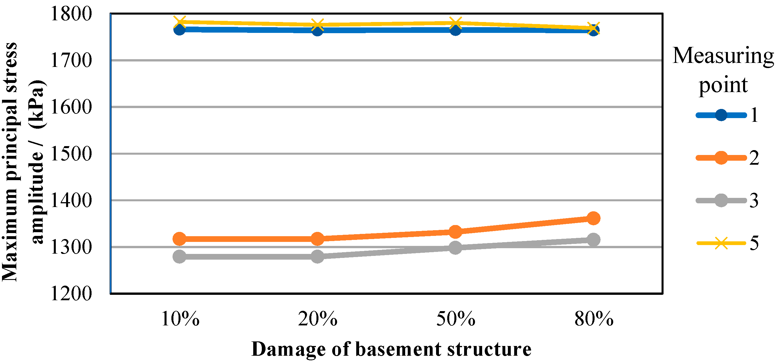
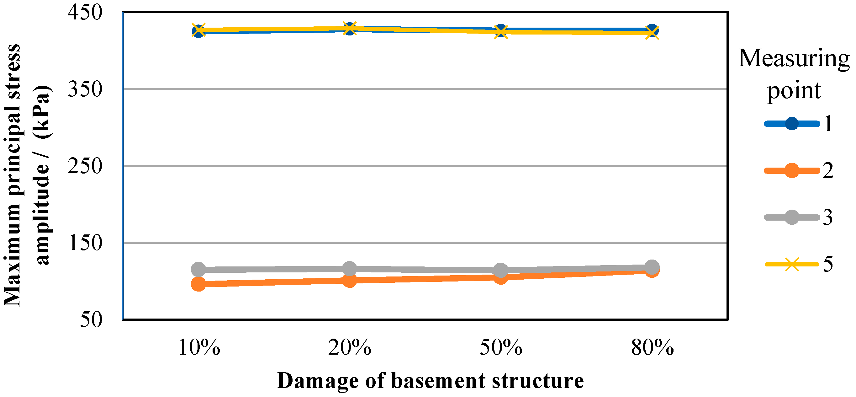
Figure 20.
Maximum principal stress amplitude diagram of measuring points 1, 2, 3, and 5 under different degrees of damage to the basement structure.
Figure 20.
Maximum principal stress amplitude diagram of measuring points 1, 2, 3, and 5 under different degrees of damage to the basement structure.
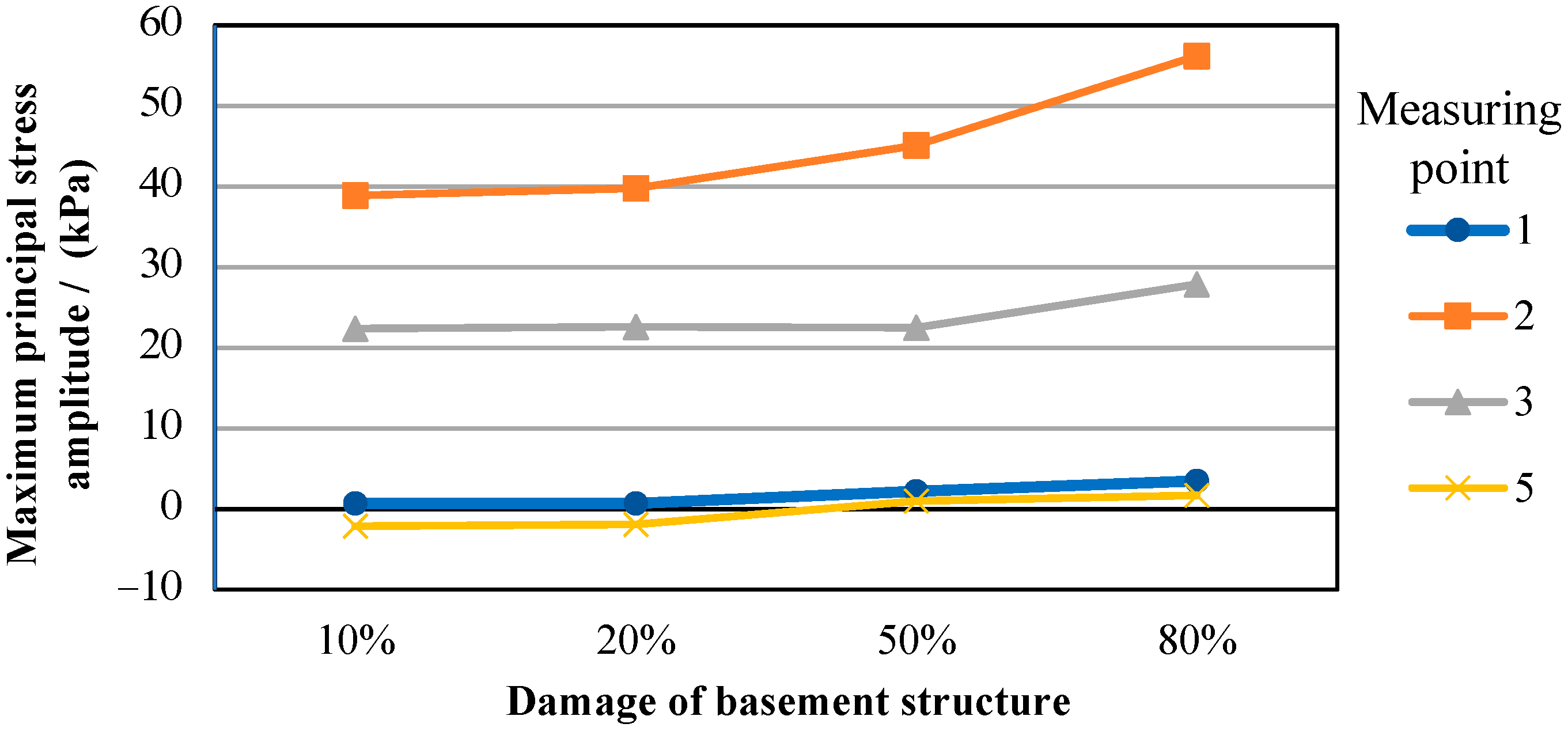
Figure 21.
Maximum principal stress increment amplitude diagram of measuring points 1, 2, 3, and 5 under different degrees of damage to the basement structure.
Figure 21.
Maximum principal stress increment amplitude diagram of measuring points 1, 2, 3, and 5 under different degrees of damage to the basement structure.
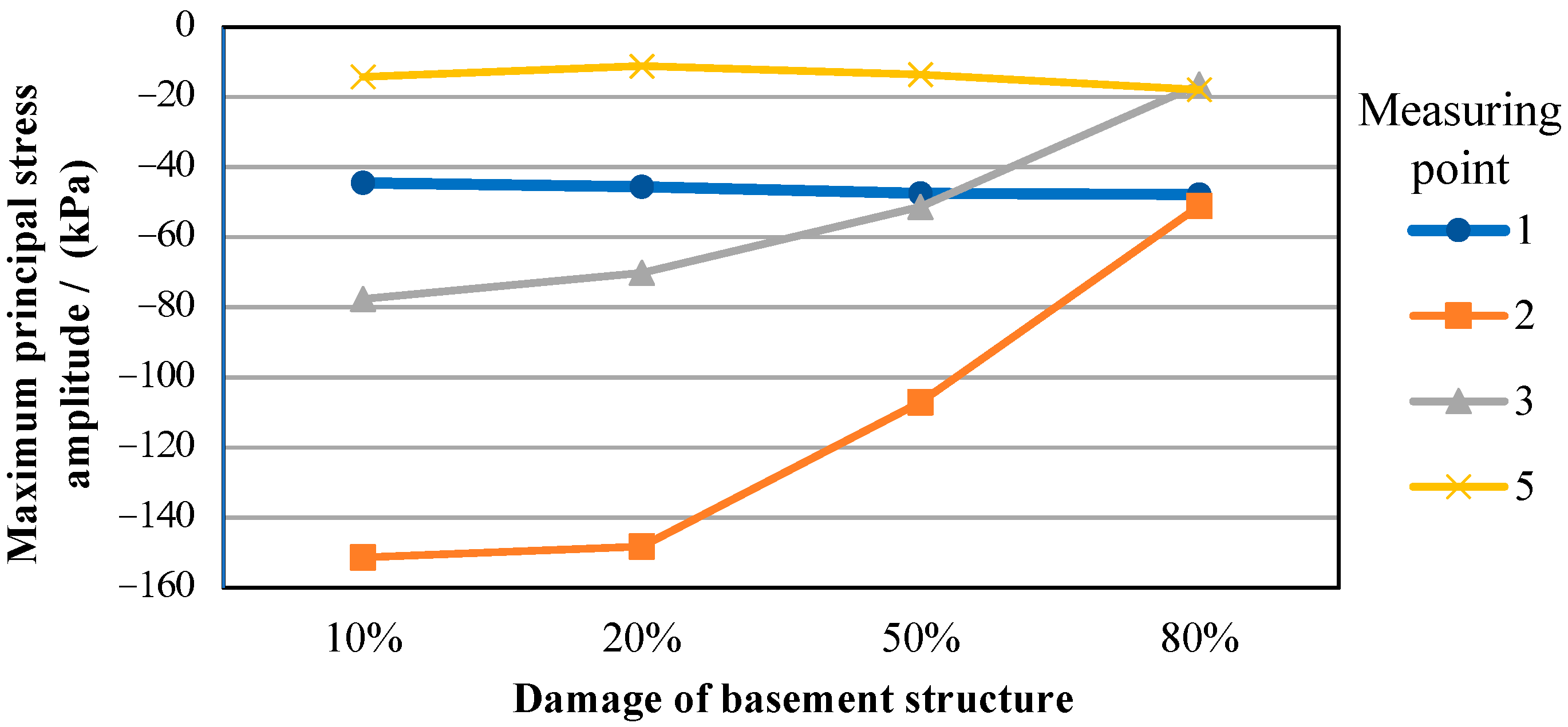
Figure 22.
Minimum principal stress amplitude diagram of measuring points 1, 2, 3, and 5 under different degrees of damage to the basement structure.
Figure 22.
Minimum principal stress amplitude diagram of measuring points 1, 2, 3, and 5 under different degrees of damage to the basement structure.
Figure 23.
Minimum principal stress increment amplitude diagram of measuring points 1, 2, 3, and 5 under different degrees of damage to the basement structure.
Figure 23.
Minimum principal stress increment amplitude diagram of measuring points 1, 2, 3, and 5 under different degrees of damage to the basement structure.
Table 1.
Simulation parameters of the uniaxial tensile test.
Table 1.
Simulation parameters of the uniaxial tensile test.
| | | | |
|---|
| 3.1 × 10⁴ | 3.48 | 1.0 | 0.518 | 0.52 |
Table 2.
Simulation parameters of uniaxial compression test.
Table 2.
Simulation parameters of uniaxial compression test.
| | | | |
|---|
| 3.17 × 10⁴ | 10.2 | 1.0 | 0.16 | 0.42 |
Table 3.
Simulation parameters of biaxial stress test.
Table 3.
Simulation parameters of biaxial stress test.
| | | | |
|---|
| 3.10 × 10⁴ | 15.0 | 1.0 | 0.19 | 0.37 |
Table 4.
Simulation parameters of the cyclic tensile test.
Table 4.
Simulation parameters of the cyclic tensile test.
| | | | |
|---|
| 3.17 × 10⁴ | 3.47 | 1.0 | 0.518 | 0.52 |
Table 5.
Simulation parameters of cyclic compression test.
Table 5.
Simulation parameters of cyclic compression test.
| | | | |
|---|
| 3.0 × 10⁴ | 13.8 | 1.0 | 0.16 | 0.42 |
Table 6.
Calculation cases with different design parameters of the tunnel base structure.
Table 6.
Calculation cases with different design parameters of the tunnel base structure.
| Influence Factor | Grade of Surrounding Rock | Thickness Invert | Rise Span Ratio of Invert |
|---|
| Specific parameters | III | 30 cm | 1/15 |
| IV | 40 cm | 1/12 |
| V | 50 cm | 1/10 |
| VI | 60 cm | 1/8 |
Table 7.
Basic mechanical parameters of concrete and surrounding rock.
Table 7.
Basic mechanical parameters of concrete and surrounding rock.
| Structure | Elasticity Modulus/GPa | Poisson’s Ratio | Weight/(kN·m−3) | Cohesion/kPa | Friction Angle/° |
|---|
| Ballast | 32.0 | 0.18 | 25.0 | / | / |
| Filling layer | 29.0 | 0.18 | 25.0 | / | / |
| Invert | 30.0 | 0.18 | 25.0 | / | / |
| Second lining | 30.0 | 0.18 | 25.0 | / | / |
| First branch | 27.5 | 0.18 | 25.0 | / | / |
| Surrounding rock | 1.5 | 0.36 | 19.5 | 200 | 42 |
Table 8.
Mechanical damage parameters of concrete.
Table 8.
Mechanical damage parameters of concrete.
| Structure | | | | | | | |
|---|
| Ballast | 8.44 | 1.26 | 1.15 | 0.23 | 1.0 | 0.58 | 0.35 |
| Filling layer | 4.76 | 0.89 | 0.98 | 0.16 | 1.0 | 0.51 | 0.41 |
| Invert | 6.68 | 1.10 | 1.05 | 0.18 | 1.0 | 0.54 | 0.39 |
| Second lining | 6.68 | 1.10 | 1.05 | 0.18 | 1.0 | 0.54 | 0.39 |
| First branch | 3.84 | 0.77 | 0.94 | 0.14 | 1.0 | 0.46 | 0.43 |
Table 9.
Track geometry irregularity management value in the UK.
Table 9.
Track geometry irregularity management value in the UK.
| Control Conditions | Wavelength/m | Normal Vector/mm |
|---|
| According to ride comfort ① | 50.00 | 16.00 |
| 20.00 | 9.00 |
| 10.00 | 5.00 |
| According to the dynamic additional load acting on the line ② | 5.00 | 2.50 |
| 2.00 | 0.60 |
| 1.00 | 0.30 |
| Wave abrasion ③ | 0.50 | 0.10 |
| 0.05 | 0.005 |
Table 10.
Horizontal dynamic stress amplitudes of measuring points 2, 3, and 4 under different softening degrees of the basement surrounding rock.
Table 10.
Horizontal dynamic stress amplitudes of measuring points 2, 3, and 4 under different softening degrees of the basement surrounding rock.
| Measuring Point | Horizontal Dynamic Stress Amplitude/kPa under Different Softening Degrees of the Basement Surrounding Rock |
|---|
| 30% Reduction | 50% Reduction | 80% Reduction | 90% Reduction |
|---|
| 2 | −177.9 | −186.6 | −214.6 | −240.8 |
| 3 | −93.6 | −101.7 | −117.4 | −139.1 |
| 4 | −37.6 | −38.7 | −47.9 | −58.8 |
Table 11.
Horizontal dynamic stress amplitudes of measuring points 2, 3, and 4 under different basement hanging ranges.
Table 11.
Horizontal dynamic stress amplitudes of measuring points 2, 3, and 4 under different basement hanging ranges.
| Measuring Point | Horizontal Dynamic Stress Amplitude/kPa under Different Basement Hanging Ranges |
|---|
| 1/4 Width Loading Line | 1/2 Width Empty Line | 1/2 Width Loading Line | 3/4 Width Loading Line |
|---|
| 2 | −211.8 | −184.9 | −264.3 | −332.2 |
| 3 | −93.7 | −123.3 | −119.8 | −216.5 |
| 4 | −37.6 | −82.5 | −31.6 | −55.3 |
Table 12.
Horizontal dynamic stress amplitudes of measuring points 2, 3, and 4 under different degrees of damage to the foundation structure.
Table 12.
Horizontal dynamic stress amplitudes of measuring points 2, 3, and 4 under different degrees of damage to the foundation structure.
| Measuring Point | Horizontal Dynamic Stress Amplitude/kPa under Different Degrees of Damage to the Basement Structure |
|---|
| 10% Reduction | 20% Reduction | 50% Reduction | 80% Reduction |
|---|
| 2 | −147.8 | −138.3 | −106.8 | −51.2 |
| 3 | −76.4 | −71.9 | −47.9 | −16.7 |
| 4 | −31.2 | −27.5 | −17.7 | −6.2 |
Table 13.
Maximum principal stress amplitude of measuring points 1, 2, 3, and 5 under different softening degrees of basement surrounding rock.
Table 13.
Maximum principal stress amplitude of measuring points 1, 2, 3, and 5 under different softening degrees of basement surrounding rock.
| Measuring Point | Maximum Principal Stress Amplitude/kPa under Different Softening Degrees of Basement Surrounding Rock |
|---|
| Maximum Principal Stress | Maximum Principal Stress Increment |
|---|
| 30% | 50% | 80% | 90% | 30% | 50% | 80% | 90% |
|---|
| 1 | 421 | 387 | 346 | 329 | −2.7 | −1.9 | 1.4 | 2.1 |
| 2 | 109 | 138 | 162 | 168 | 35.8 | 31.8 | 28.5 | 24.9 |
| 3 | 111 | 96 | 98 | 103 | 21.6 | 20.2 | 18.8 | 16.9 |
| 5 | 437 | 386 | 341 | 321 | 0.5 | −1.2 | −1.1 | −0.6 |
Table 14.
Minimum principal stress amplitude of measuring points 1, 2, 3, and 5 under different softening degrees of basement surrounding rock.
Table 14.
Minimum principal stress amplitude of measuring points 1, 2, 3, and 5 under different softening degrees of basement surrounding rock.
| Measuring Point | Minimum Principal Stress Amplitude/kPa under Different Softening Degrees of Basement Surrounding Rock |
|---|
| Minimum Principal Stress | Minimum Principal Stress Increment |
|---|
| 30% | 50% | 80% | 90% | 30% | 50% | 80% | 90% |
|---|
| 1 | 1706 | 1615 | 1471 | 1407 | −55.5 | −52.3 | −49.2 | −53.6 |
| 2 | 1478 | 1748 | 2206 | 2342 | −171.2 | −187.6 | −215.8 | −240.1 |
| 3 | 1382 | 1576 | 2047 | 2226 | −95.3 | −98.4 | −117.9 | −136.2 |
| 5 | 1727 | 1639 | 1498 | 1425 | −11.5 | −10.1 | −8.4 | −6.5 |
Table 15.
Maximum principal stress amplitude of measuring points 1, 2, 3, and 5 under different basement hanging ranges.
Table 15.
Maximum principal stress amplitude of measuring points 1, 2, 3, and 5 under different basement hanging ranges.
| Measuring Point | Maximum Principal Stress Amplitude/kPa under Different Basement Hanging Ranges |
|---|
| Maximum Principal Stress | Maximum Principal Stress Increment |
|---|
| 1/4 Width Loading Line | 1/2 Width Empty Line | 1/2 Width Loading Line | 3/4 Width Loading Line | 1/4 Width Loading Line | 1/2 Width Empty Line | 1/2 Width Loading Line | 3/4 Width Loading Line |
|---|
| 1 | 415 | 436 | 357 | 346 | −2.2 | −6.4 | 4.6 | 3.9 |
| 2 | 11 | 212 | −9 | −16 | 8.7 | 40.3 | 8.9 | −20.5 |
| 3 | 246 | 508 | 286 | −17 | 35.2 | −17.6 | 3.7 | −1.3 |
| 5 | 437 | 353 | 435 | 287 | −0.8 | 4.5 | −7.4 | −31.6 |
Table 16.
Minimum principal stress amplitude of measuring points 1, 2, 3, and 5 under different basement hanging ranges.
Table 16.
Minimum principal stress amplitude of measuring points 1, 2, 3, and 5 under different basement hanging ranges.
| Measuring Point | Minimum Principal Stress Amplitude/kPa under Different Basement Hanging Ranges |
|---|
| Minimum Principal Stress | Minimum Principal Stress Increment |
|---|
| 1/4 Width Loading Line | 1/2 Width Empty Line | 1/2 Width Loading Line | 3/4 Width Loading Line | 1/4 Width Loading Line | 1/2 Width Empty Line | 1/2 Width Loading Line | 3/4 Width Loading Line |
|---|
| 1 | 1638 | 2009 | 1259 | 1279 | −58.1 | −57.2 | 14.6 | 19.2 |
| 2 | 1590 | 2106 | 1397 | 176 | −206.3 | −186.4 | −265.8 | −296.7 |
| 3 | 1547 | 1947 | 2332 | 492 | −94.5 | −135.3 | −94.9 | −198.4 |
| 5 | 1819 | 1235 | 2041 | 2154 | −11.8 | −18.2 | −5.8 | 13.3 |
Table 17.
Maximum principal stress amplitude of measuring points 1, 2, 3, and 5 under different degrees of damage to the basement structure.
Table 17.
Maximum principal stress amplitude of measuring points 1, 2, 3, and 5 under different degrees of damage to the basement structure.
| Measuring Point | Maximum Principal Stress Amplitude/kPa under Different Degrees of Damage to the Basement Structure |
|---|
| Maximum Principal Stress | Maximum Principal Stress Increment |
|---|
| 10% | 20% | 50% | 80% | 10% | 20% | 50% | 80% |
|---|
| 1 | 425 | 428 | 426 | 426 | 0.7 | 0.7 | 2.2 | 3.5 |
| 2 | 96 | 101 | 105 | 114 | 38.9 | 39.8 | 45.1 | 56.2 |
| 3 | 115 | 116 | 114 | 118 | 22.4 | 22.6 | 22.5 | 27.9 |
| 5 | 427 | 429 | 424 | 423 | −2.1 | −1.9 | 1.0 | 1.7 |
Table 18.
Minimum principal stress amplitude of measuring points 1, 2, 3, and 5 under different degrees of damage to the basement structure.
Table 18.
Minimum principal stress amplitude of measuring points 1, 2, 3, and 5 under different degrees of damage to the basement structure.
| Measuring Point | Minimum Principal Stress Amplitude/kPa under Different Degrees of Damage to the Basement Structure |
|---|
| Minimum Principal Stress | Minimum Principal Stress Increment |
|---|
| 10% | 20% | 50% | 80% | 10% | 20% | 50% | 80% |
|---|
| 1 | 1766 | 1764 | 1765 | 1764 | −44.5 | −45.6 | −47.5 | −47.8 |
| 2 | 1317 | 1317 | 1332 | 1361 | −151.3 | −148.2 | −107.1 | −51.1 |
| 3 | 1279 | 1279 | 1298 | 1315 | −77.6 | −70.2 | −51.3 | −16.5 |
| 5 | 1782 | 1776 | 1780 | 1769 | −14.3 | −11.2 | −13.6 | −17.9 |


