Abstract
Based on the present studies about the application of approximative fractional Brownian motion in the European option pricing models, our goal in the article is that we adopt the creative model by adding approximative fractional stochastic volatility to double Heston model with jumps since approximative fractional Brownian motion is more proper for application than Brownian motion in building option pricing models based on financial market data. We are the first to adopt the creative model. We derive the pricing formula for the options and the formula for the characteristic function. We also estimate the parameters with the loss function for the model and two nested models and compare the performance among those models based on the market data. The outcome illustrates that the model offers the best performance among the three models. It demonstrates that approximative fractional Brownian motion is more proper for application than Brownian motion.
1. Introduction
We aim to derive European option pricing formula under the framework of double Heston model including approximative fractional stochastic volatility and jumps. Considering the present studies, we are first to adopt this creative model. Option pricing has become a crucial issue in financial modeling since Black and Scholes [1] did the creative work in this field. However, the assumption that the volatility is a random variable is more appropriate than constant volatility assumption since the market data shows that the volatility smile exists. Meanwhile, some studies have presented that stochastic volatility models given the interpretation about volatility smile. Therefore, the models under this framework have become an essential issue in the field of option pricing. The most favored stochastic volatility model is the Heston [2] model. The Cox-Ingersoll-Ross (CIR) [3] process is adopted in the model. The model has advantages of mean-reverting and non-negative characteristics. Another advantage of the model is that it only needs to explore the characteristic functions for obtaining the pricing formula for the options. Schöbel and Zhu [4] also presented a stochastic volatility model. Compared with Heston [2], they explored the characteristic functions with a new approach which is called expectation approach that they obtained the solution for the characteristic functions directly by deriving the expectation functions. In some cases, one-factor volatility process cannot explain the shape of the volatility smile, and therefore is not always suitable to be adopted in building option pricing models. Christoffersen et al. [5] claimed that since the correlation between the stock returns and variance could be nonconstant, one-factor models cannot interpret the shape of the volatility smile. One way to solve this issue is to build two-factor models. Based on results from the one-factor model, they presented a two-factor model to describe the variance process. Their empirical results demonstrated that their model provides more flexibility in modeling the shape of the smile and the term structure of the volatility. Moreover, the two factors represent the relationships between short-term returns, long-term returns and the variance respectively. Therefore, the models under this framework have also become an essential issue in the field of option pricing.
Jumps explain the discontinuous nature. Merton [6] presented that empirical data shows the existence of the discontinuous behavior, and therefore developed a model with lognormally distributed jumps. Kou [7] developed a model with double exponentially distributed jumps. It has the characteristics of explaining the leptokurtic feature and smile. Besides the European options, it can also provide explanations and solutions for other types of derivatives. Some empirical studies have showed that jumps are needed to improve the performance of the models. Bates [8] developed a stochastic volatility model with lognormally distributed jumps. The empirical study demonstrated that jumps can capture the volatility smile and the models under this framework can offer reasonable prices. Bakshi et al. [9] presented several models including stochastic volatility model with lognormally distributed jumps to explore the performance among those several models. They found that the model with stochastic volatility has limit in pricing short-term options and the model with jumps has more flexibility than it. Their empirical study also demonstrated that stochastic volatility model with jumps gives better performance on short-term options.
With regard to the derivation of the characteristic functions, two methods are usually adopted to fulfill it. The first one is based on the affine jump-diffusion (AJD) models. Duffie et al. [10]. synthesized the option pricing models meeting some distinct requirements under the framework of the AJD models. The closed-form of the Fourier transform of the securities can be obtained by adopting the Feynman-Kac theorem. The second one is the modular method [11], it is based on expectation method [4]. To be specific, the modular method is the extension of expectation method which means that the solution of the characteristic function is a framework composed of different modules, one can use expectation method to obtain the solutions of those modules. Moreover, several authors studied foreign exchange (FX) options under option pricing models and adopted expectation method to derive the characteristic functions [12,13,14]. Based on those studies, Ahlip et al. [15] developed an option pricing model under the framework of the forward stock price. They adopted expectation method to derive the characteristic functions.
Fractional Brownian motion has become an important engine in financial modeling since it has characteristics of self-similarity and long-range dependence to coincide with financial data. It has also been discussed in other fields [16]. The name of it was first given by Mandelbrot and Van Ness [17]. They presented the expression of it with a stochastic integral. It is a Gaussian process with a Hurst parameter [18]. Though it can replace Brownian motion in modeling the dynamics of stock price, it was proved to have the possibility of arbitrage [19]. Moreover, since one cannot apply Itô theory on it, Wick products were adopted to study it [18]. However, Björk and Hult [20] proved that the model is lack of the economic explanation. There are two methods to solve this issue. The first method is to adopt the mixed fractional Brownian motion as a substitute. Cheridito [21] has proved that if the Hurst parameter is in a specific interval, it is equivalent to Brownian motion. Several authors developed option pricing models with the mixed fractional Brownian motion [22,23]. It can also be applied in building FX option pricing models [24,25]. The second method is to use approximative fractional Brownian motion as a substitute and it was developed by Thao [26]. Fractional Brownian motion can be presented with two terms and the gamma function, since the first one has continuous trajectories, one can only consider the second one with the characteristic of long-range dependence [26]. Thao [26] approximated the second term with approximative fractional Brownian motion. Thao [26] has proved that approximative fractional Brownian motion is a semi-martingale. Besides modeling the dynamics of stock price with the above three kinds of motions, one can also model the dynamics of the volatility with them. Fractional Brownian motion has been discussed in stochastic volatility models [27]. Approximative fractional Brownian motion has also been used in building stochastic volatility models in recent years. Intarasit and Sattayatham [28] adopted an approximation of fractional stochastic volatility model with jumps. The simulation showed that the performance of the model is better than the stochastic volatility model with jumps. Sattayatham and Intarasit [29] developed a model by adopting an approximation of fractional stochastic volatility model with jumps. They derived pricing formula for the options. Several authors offered empirical results that they used market prices for calibration [30,31]. Some authors also developed option pricing model with approximative fractional Brownian motion under a creative framework. Kang et al. [32] presented a FX option pricing model, and the dynamics of FX and the variance are specified with an approximative fractional process.
In consideration of the present studies, we adopt a double Heston model with approximative fractional stochastic volatility and jumps. We are first to adopt the creative model. We derive the pricing formula, estimate the parameters with the loss function for the model and two nested models and compare the performance among those models. Our innovation in the article is that we adopt this creative model by adding approximative fractional stochastic volatility to double Heston model with jumps since no one has developed this model before.
2. The Model
We present some specific knowledge about approximative fractional Brownian motion. We present some review of fractional Brownian motion with the Hurst index in the first place. It is a Gaussian process with zero mean and the following covariance . It coincides with standard Brownian motion when . When , it exhibits long-range dependence, so one can only consider the situation when for financial studies. It is also known to have the following expression [17]
where , indicates standard Brownian motion, and indicates the gamma function. One can only deal with since it exhibits the characteristic of long-range dependence [26,29,30,31]. The approximation of is which can be expressed as [26]
where is an approximative fractional Brownian motion. as and is a semi-martingale, the proof can be found in Thao [26]. It can also be expressed as
where H indicates the long-memory parameter, indicates the positive approximation factor. is a stochastic processes expressed as
where and , are independent standard Brownian motions.
Let be a probability space. is the filtration and is the risk-neutral probability measure. Stock price process and variance processes , are given by the following dynamics
where and are mean reversion rates, and are mean reversion levels, and are the volatilities of the variances. , are correlated Brownian motions that . , are correlated Brownian motions that . denotes Poisson process, denotes the intensity, and J denotes jump size. follows an asymmetric double exponential distribution with the density
where , , . p and q are the probabilities for upward and downward abnormalities. One can get the following equation .
We give the call option pricing formula by using Radon-Nikodym derivative and the expression of the characteristic function. The call option price under is the expectation of the discounted value of the payoff
where , , and K is the strike.
We convert to the measure by applying the Radon-Nikodym derivative [33]
where .
Accordingly, we can have the following expression
The density function and the characteristic function satisfy the following equations
and we define
where denotes the characteristic function under and denotes the characteristic function under . We adopt the Radon-Nikodym derivative to have
Accordingly, we can have the following expression
Accordingly, we only need to derive the formula for to have the pricing formula.
3. The Characteristic Function
We give the derivation on the characteristic function formula in this part.
Theorem 1.
If the asset price follows the process expressed in the dynamics of the model, the formula for is expressed as
where
Proof of Theorem 1.
satisfies the following PIDE using Feynman-Kac theorem according to Christoffersen et al. [5] and Pospíšil and Sobotka [31]
We speculate that is under the following framework
with initial conditions , , and . Reorganizing the above PIDE, we can have the following expression
where .
Since is martingale and , we have four differential equations by sorting out the similar items in the above equation
We can have the formulae for , , and by dealing with the solutions of the above equations. Accordingly, we can have the solution of . The proof is complete. □
4. Calibration
The loss function is usually adopted to estimate the parameters in option pricing models and the goal is to minimize the value of it [33]. It relates to the error between the market and model prices or implied volatilities. It means one can estimate the parameters in option pricing models as long as one can obtain the market prices or implied volatilities. When one can obtain the market implied volatilities, the loss functions usually used are to minimize the absolute and relative value of the mean-squared error (MSE) between market and model implied volatilities. When one can obtain the market prices, there are two loss functions one usually uses to estimate the parameters. The first loss function is to minimize the absolute value of MSE between market and model prices, the other one is to minimize the relative value of MSE between market and model prices. Because there is a high weight on the assignment for the options with high values in the first function, sometimes the second loss function is the first choice [34]. Some authors also developed some new loss functions. The absolute value of the error, the absolute value of the root squared error and the squared error between the ask and bid market prices can be considered to be the weights [31]. The Black-Scholes sensitivity can also be considered to be the weight [5]. Rouah [33] developed a loss function based on the first loss function that he considered the market prices as the denominator. There is no consensus between the authors about which loss function is the best one to estimate the parameters, but one should consider the consistency when using the loss functions. In the first place, the loss function for estimation and evaluation should be identical among different models. In the second place, one should adopt the same loss function when comparing the effects of different option pricing models [34].
In this section, we adopt the market data to calibrate the parameters for three models. The loss function that is to minimize the absolute value of MSE between the market and model prices is adopted in the calibration. We consider the market prices of S&P 500 index call options quoted on 3 January 2019, we obtain the market data from the website of CBOE. We choose 0.024 to be the risk-free interest rate and fix = 1. We follow some principles to filter the market data. We eliminate the call options with zero trading volume and the call options with prices lower than 3 to alleviate the impact of the discreteness on valuation. We eliminate the call options violating the arbitrage restriction [9]. We also impose some restrictions on the maturities that we choose the maturities bigger than 30 days and smaller than 365 days, and therefore there are six maturities in the market data. The parameters we need to calibrate are given by
Assuming that we have a set of N call options, the market prices are (), we can obtain the model prices () with needed for calibration. The approach to calibrate is to adopt the loss function
We also adopt a criterion for the performance on calibration, we adopt the root mean-squared error (RMSE) which is given by the following equation
The estimation outcome is illustrated in Table 1. It shows that the model gives the smallest RMSE, and the double Heston model gives better approximation than the Heston model. The estimation outcomes of the double Heston model and the model are also in accordance with the results in Christoffersen et al. [5] that the two factors of the variance have different mean reversion levels and they show the correlations between the two returns and the variance. We also plot the market implied volatilities and the model implied volatilities to compare the effects of different models based on the market data [35]. We adopt the bisection algorithm [33] to discover the market and model implied volatilities. Because the Heston model gives the worst performance on RMSE among the three models, we only plot the market implied volatilities, double Heston model and the model implied volatilities to compare the effects of the two models for the maturities. Figure 1 demonstrates the outcome, the horizontal axis represents the strikes and the vertical axis represents implied volatilites. It illustrates that the model gives better approximation than double Heston model in accordance with the market implied volatilities for almost all the maturities.

Table 1.
Calibration results of the parameters.
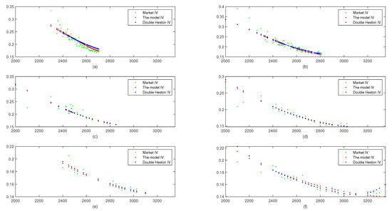
Figure 1.
Market and model implied volatilities for different maturities. (a) Maturity 43 days. (b) Maturity 71 days. (c) Maturity 105 days. (d) Maturity 169 days. (e) Maturity 260 days. (f) Maturity 351 days.
5. Conclusions
Fractional Brownian motion has become an important tool in financial modeling since it has the characteristics of self-similarity and long-range dependence to coincide with financial data. Though it can replace Brownian motion in modeling the dynamics of stock price, it was proved to be lacking the economic explanation. One method to solve this problem is to use approximative fractional Brownian motion as a substitute. Besides modeling the dynamics of a stock price with the above motions, one can also model the dynamics of the volatility with them. Fractional Brownian motion has been discussed in stochastic volatility models. Approximative fractional Brownian motion has also been used in building stochastic volatility models in recent years. Therefore, in consideration of the present studies about the application of it in the European option pricing models, we adopted a double Heston model with approximative fractional stochastic volatility and jumps. We are first to adopt the creative model. We did some pioneering work to fill the gap in developing European option pricing models. To be specific, our contribution in the article is that we adopted this creative model by adding approximative fractional stochastic volatility to double Heston model with jumps since no one has developed this model before. We derived the pricing formula and the characteristic function formula. We estimated the parameters with the loss function and compared the performance of different models on the call option prices. The outcome illustrates that the model gives the smallest RMSE, double Heston model gives better approximation than the Heston model. The estimation outcomes of double Heston model and the model are also in accordance with the results in Christoffersen et al. [5] that the two factors of the variance show the correlations between the different returns and the variance. We also plotted the market implied volatilities and the model implied volatilities to compare the effects of different models based on the market data. Because the Heston model gives the worst performance among the three models on RMSE, we only plotted the market implied volatilities, double Heston model and the model implied volatilities to compare the effects of the two models for the maturities. The outcome illustrates that the model offers better approximation than double Heston model in accordance with the market implied volatilities for almost all the maturities. Based on the market data on one day, it shows that approximative fractional Brownian motion maybe more proper for financial application than Brownian motion. However, the model may have different performance based on other market data that it may perform better or worse than the other models. Therefore, some other models also based on approximative fractional Brownian motion can be developed in the future.
Author Contributions
Conceptualization, Y.C., Y.W. and S.Z.; data curation, Y.C., Y.W. and S.Z.; formal analysis, Y.C., Y.W. and S.Z.; funding acquisition, Y.W. and S.Z.; investigation, Y.C.; methodology, Y.C., Y.W. and S.Z.; project administration, Y.W. and S.Z.; resources, Y.C.; software, Y.C., Y.W. and S.Z.; supervision, Y.W. and S.Z.; validation, Y.W. and S.Z.; visualization, Y.C., Y.W. and S.Z.; Writing—original draft, Y.C.; Writing—review editing, Y.W. and S.Z. All authors have read and agreed to the published version of the manuscript.
Funding
This research was funded by the National Natural Science Foundation of China [grant number 11601420] and the Natural Science Foundation of Shaanxi Province, China [grant number 2020JM-577].
Institutional Review Board Statement
Not applicable.
Informed Consent Statement
Not applicable.
Data Availability Statement
The data used to support the findings of this study are available from the corresponding authors upon request.
Conflicts of Interest
The authors declare no conflict of interest.
References
- Black, F.; Scholes, M. The pricing of options and corporate liabilities. J. Polit. Econ. 1973, 81, 637–654. [Google Scholar] [CrossRef]
- Heston, S. A closed-form solution for options with stochastic volatility with application to bond and currency options. Rev. Financ. Stud. 1993, 6, 327–343. [Google Scholar] [CrossRef]
- Cox, J.C.; Ingersoll, J.E.; Ross, S.A. A theory of the term structure of interest rates. Econometrica 1985, 53, 385–407. [Google Scholar] [CrossRef]
- Schöbel, R.; Zhu, J.W. Stochastic volatility with an Ornstein-Uhlenbeck process: An extension. Rev. Financ. 1999, 3, 23–46. [Google Scholar] [CrossRef]
- Christoffersen, P.; Heston, S.; Jacobs, K. The shape and term structure of the index option smirk: Why multifactor stochastic volatility models work so well. Manag. Sci. 2009, 55, 1914–1932. [Google Scholar] [CrossRef]
- Merton, R. Option pricing when underlying stock returns are discontinuous. J. Financ. Econ. 1976, 3, 125–144. [Google Scholar] [CrossRef]
- Kou, S.G. A jump-diffusion model for option pricing. Manag. Sci. 2002, 48, 1086–1101. [Google Scholar] [CrossRef]
- Bates, D. Jumps and stochastic volatility: Exchange rate processes implicit in deutsche mark options. Rev. Financ. Stud. 1996, 9, 69–107. [Google Scholar] [CrossRef]
- Bakshi, G.; Cao, C.; Chen, Z. Empirical performance of alternative option pricing models. J. Financ. 1997, 52, 2003–2049. [Google Scholar] [CrossRef]
- Duffie, D.; Pan, J.; Singleton, K. Transform analysis and asset pricing for affine jump-diffusions. Econometrica 2000, 68, 1343–1376. [Google Scholar] [CrossRef]
- Zhu, J. Stochastic volatility models. In Applications of Fourier Transform to Smile Modeling: Theory and Implementation; Springer: Berlin/Heidelberg, Germeny, 2010; pp. 45–76. [Google Scholar]
- Ahlip, R. Foreign exchange options under stochastic volatility and stochastic interest rates. Int. J. Theor. Appl. Financ. 2008, 11, 277–294. [Google Scholar] [CrossRef]
- Ahlip, R.; Rutkowski, M. Pricing of foreign exchange options under the Heston stochastic volatility model and CIR interest rates. Quant. Financ. 2013, 13, 955–966. [Google Scholar] [CrossRef]
- Ahlip, R.; Park, L.A.F.; Prodan, A. Pricing currency options in the Heston/CIR double exponential jump-diffusion model. Int. J. Financ. Eng. 2017, 4, 1–30. [Google Scholar] [CrossRef]
- Ahlip, R.; Park, L.A.F.; Prodan, A. Semi-Analytical option pricing under double Heston jump-diffusion hybrid model. J. Math. Sci. Model. 2018, 1, 138–152. [Google Scholar] [CrossRef]
- Wang, W.; Seno, F.; Sokolv, L.M.; Chechkin, A.V.; Metzler, R. Unexpected crossovers in correlated random-diffusivity processes. New. J. Phys. 2020, 22, 1–16. [Google Scholar] [CrossRef]
- Mandelbrot, B.B.; Van Ness, J.W. Fractional Brownian motions, fractional noises and applications. SIAM Rev. 1968, 10, 422–437. [Google Scholar] [CrossRef]
- Hu, Y.; Øksendal, B. Fractional white noise calculus and application to finance. Infin. Dimens. Anal. Quantum Probab. Relat. Top. 2003, 6, 1–32. [Google Scholar] [CrossRef]
- Rogers, L.C.G. Arbitrage with fractional Brownian motion. Math. Financ. 1997, 7, 95–105. [Google Scholar] [CrossRef]
- Björk, T.; Hult, H. A note on Wick products and the fractional Black-Scholes model. Finance Stoch. 2005, 9, 197–209. [Google Scholar] [CrossRef]
- Cheridito, P. Mixed fractional Brownian motion. Bernoulli 2001, 7, 913–934. [Google Scholar] [CrossRef]
- Wang, X.; Zhu, E.; Tang, M.; Yan, H. Scaling and long-range dependence in option pricing II: Pricing European option with transaction costs under the mixed Brownian-fractional Brownian model. Physica A 2010, 389, 445–451. [Google Scholar] [CrossRef]
- Guo, Z.; Yuan, H. Pricing European option under the time-changed mixed Brownian-fractional Brownian model. Physica A 2014, 406, 73–79. [Google Scholar] [CrossRef]
- Sun, L. Pricing currency options in the mixed fractional Brownian motion. Physica A 2013, 392, 3441–3458. [Google Scholar] [CrossRef]
- Kim, K.; Yun, S.; Kim, N.; Ri, J. Pricing formula for European currency option and exchange option in a generalized jump mixed fractional Brownian motion with time-varying coefficients. Physica A 2019, 522, 215–231. [Google Scholar] [CrossRef]
- Thao, T.H. An approximate approach to fractional analysis for finance. Nonlinear Anal. Real World Appl. 2006, 7, 124–132. [Google Scholar] [CrossRef]
- El Euch, O.; Rosenbaum, M. The characteristic function of rough Heston models, Mathematical Finance. Math. Financ. 2019, 29, 3–38. [Google Scholar] [CrossRef]
- Intarasit, A.; Sattayatham, P. A geometric Brownian motion model with compound Poisson process and fractional stochastic volatility. Adv. Appl. Stat. 2010, 16, 25–47. [Google Scholar]
- Sattayatham, P.; Intarasit, A. An approximate formula of European option for fractional stochastic volatility jump-diffusion model. J. Math. Stat. 2011, 7, 230–238. [Google Scholar] [CrossRef]
- Mrázek, M.; Pospíšil, J.; Sobotka, T. On calibration of stochastic and fractional stochastic volatility models. Eur. J. Oper. Res. 2016, 254, 1036–1046. [Google Scholar]
- Pospíšil, J.; Sobotka, T. Market calibration under a long memory stochastic volatility model. Appl. Math. Financ. 2016, 23, 323–343. [Google Scholar]
- Kang, J.; Yang, B.; Huang, N. Pricing of FX options in the MPT/CIR jump-diffusion model with approximative fractional stochastic volatility. Physica A 2019, 532, 121871. [Google Scholar] [CrossRef]
- Rouah, F.D. Parameter estimation. In The Heston Model and Its Extensions in Matlab and C#; John Wiley & Sons: Hoboken, NJ, USA, 2013; pp. 147–176. [Google Scholar]
- Christoffersen, P.; Jacobs, K. The Heston model for European options and The importance of the loss function in option valuation. J. Financ. Econ. 2004, 72, 291–318. [Google Scholar] [CrossRef]
- Zhong, Y.; Bao, Q.; Li, S. FX options pricing in logarithmic mean-reversion jump-diffusion model with stochastic volatility, Applied Mathemamtics and Computation. Appl. Math. Comput. 2015, 251, 1–13. [Google Scholar]
Publisher’s Note: MDPI stays neutral with regard to jurisdictional claims in published maps and institutional affiliations. |
© 2021 by the authors. Licensee MDPI, Basel, Switzerland. This article is an open access article distributed under the terms and conditions of the Creative Commons Attribution (CC BY) license (http://creativecommons.org/licenses/by/4.0/).