Demographic Dynamics in Multitype Populations with Migrations

Abstract

This research work deals with mathematical modeling in complex biological systems in which several types of individuals coexist in various populations. Migratory phenomena among the populations are allowed. We propose a class of mathematical models to describe the demographic dynamics of these type of complex systems. The probability model is defined through a sequence of random matrices in which rows and columns represent the various populations and the several types of individuals, respectively. We prove that this stochastic sequence can be studied under the general setting provided by the multitype branching process theory. Probabilistic properties and limiting results are then established. As application, we present an illustrative example about the population dynamics of biological systems formed by long-lived raptor colonies.

1. Introduction

The motivation behind this research is the interest in developing new classes of mathematical models to describe the demographic dynamics of complex biological systems. We focus our attention on systems formed by several populations in which different types of individuals of the same species coexist and they can migrate to other populations of the system. Note that, in such biological systems, due to several random factors (weather conditions, food supply, fertility parameters, predators, human activities, etc.) the reproduction process occurs in a non-predictable environment. Hence, deterministic models are not appropriated to describe its demographics dynamics. On the other hand, methodologies based on population viability analysis, considered in conservation biology and in the management of threatened or endangered species (see e.g., [1] or [2]), or compartmental modeling, which has been specially applied in epidemiology, physiology, pharmacology, and other related medical sciences (see e.g., [3] or [4]), usually require information about mortality rates, growth rates, environmental variables, etc. In practice, real data about such variables are difficult to obtain. Thus, such methodologies are not usually feasible to apply. Mathematical models based on others methodologies have not been sufficiently investigated in the literature on stochastic modeling for biological systems. In this work, we will approach they from the general context provided by the multitype branching process theory.

Branching processes are mathematical models with theoretical and practical interest. They are simple to analyze and have wide applicability as models for a great variety of phenomena, especially for biological phenomena, playing a crucial role in studies on population dynamics. These studies have great importance, for instance, in population ecology, wildlife management, or conservation biology. For a detailed study on branching processes and their applications, we refer the reader to classical books, e.g., [5,6], or [7].

In particular, multitype branching processes are stochastic models describing the dynamics of populations where several types of individuals coexist and each individual, independently of the rest, can produce new individuals of all the types. The theory about such processes has been widely developed, see e.g., monograph [8]. Migratory phenomena in multitype branching processes were first considered in [9]. From then on, they have been treated by various authors under very different frameworks. For instance, branching processes with immigration as models of two-type cell populations in vivo have been investigated in [10,11]. In a genetics context, see e.g., [12], the spacial dispersion of a neutral allele has been described through multitype branching processes in which the corresponding types represent colonies among which individuals can migrate, see also [13]. By considering two-type branching processes in random environments, optimal population growth when migrations between habitats occur has been studied in [14], see also the related papers [15,16]. Multitype branching processes with immigration in a random environment have been used as model for a class of polling systems in [17].

In this paper, we consider biological systems where migratory phenomena take place among observed populations. Therefore, we know from where immigrants come and to where emigrants go. The work is structured as follows: In Section 2, we mathematically describe the class of proposed models. Section 3 is devoted to presenting the results. We first prove that the class of models introduced can be studied under the general setting provided for the theory on multitype branching processes. We then establish some probabilistic properties and limiting results. To illustrate the proposed models and results, in Section 4, we present a simulated example about the demographic dynamic of biological systems formed by several colonies of long-lived raptor species. We include the concluding remarks and some questions for research in Section 5.

2. Model Description

Consider a biological system where $d>1$ types of individuals coexist in $c>1$ geographically separated populations. Assume that, over time, migratory phenomena among populations occur. Each individual, independently of the population in which it lives, produce new individuals of all types according to certain offspring probability distribution.

Given $n\in \{0,1,\dots \}$ and $j\in \{1,\dots ,c\}$, let the random vector $X_n^j:=(X_n^{j,1},\dots ,X_n^{j,d})$, where $X_n^{j,l}$ represents the number of type-l individuals living at population j in the nth-generation, $l=1,\dots ,d$. In order to describe the demographic dynamics for this class of biological systems, we introduce the sequence ${\left\{{\mathbf{X}}_{\mathbf{n}}\right\}}_{n=0}^{\infty }$, being ${\mathbf{X}}_{\mathbf{n}}$ the $c\times d$ random matrix whose rows are the vectors $X_n^j$, $j=1\dots c$. Assuming ${\mathbf{X}}_{\mathbf{n}}$ is known, the matrix ${\mathbf{X}}_{\mathbf{n}+\mathbf{1}}$ of this stochastic sequence can be recursively determined as follows:

1.

Let ${\xi }_{n,i}^{j,k}=({\xi }_{n,i}^{j,k,1},\dots ,{\xi }_{n,i}^{j,k,d})$, $i=1,\dots ,X_n^{j,k}$; $j=1,\dots ,c$; $k=1,\dots ,d$, be independent random vectors, with ${\xi }_{n,i}^{j,k,l}$ representing the number of type-l individuals produced by the ith type-k individual living at population j in generation n. For fixed k, we also assume that:

$${\xi }_{n,i}^{j,k},i=1,\dots ,X_n^{j,k};j=1,\dots ,c;n=0,1,\dots$$

are identically distributed with probability generating function (pgf),

$$f_k\left(t\right)=f_k(t_1,\dots ,t_d):=E\left[\prod _{l=1}^d{t}_l^{{\xi }_{0,1}^{1,k,l}}\right],t=(t_1,\dots ,t_d)\in {[0,1]}^d$$

Thus, individuals of the same type reproduce according to a common offspring probability distribution, independently of the generation and the population where they live.

2.

Consider the random vector $Y_n^j=(Y_n^{j,1},\dots ,Y_n^{j,d})$, with $Y_n^{j,l}$ denoting the number of type-l individuals born at population j in generation n. Hence,

$$Y_n^j=\sum _{k=1}^d\sum _{i=1}^{X_n^{j,k}}{\xi }_{n,i}^{j,k},j=1,\dots ,c;n=0,1,\dots$$

Note that, conditioned on ${\mathbf{X}}_{\mathbf{n}}$, requirements on ${\xi }_{n,i}^{j,k}$, $j=1,\dots ,c$; $k=1,\dots ,d$; $i=1,\dots ,X_n^{j,k}$, guarantee that $Y_n^j$, $j=1,\dots ,c$, are independent and identically distributed with pgf given by:

$$E\left[\left.\prod _{k=1}^d{t}_k^{Y_n^{1,k}}\right|{\mathbf{X}}_{\mathbf{n}}\right]=\prod _{k=1}^d{\left(f_k\left(t\right)\right)}^{X_n^{1,k}},t=(t_1,\dots ,t_d)\in {[0,1]}^d$$

(1)

3.

Let us introduce the random vectors $Z_n^{j,k}=(Z_n^{j,k,1},\dots ,Z_n^{j,k,c})$, where the variable $Z_n^{j,k,l}$ is the number of individuals that emigrate to population l, among the $Y_n^{j,k}$ type-k individuals born at population j in generation n. Clearly,

$$\sum _{l=1}^c{Z}_n^{j,k,l}=Y_n^{j,k},j=1,\dots ,c;k=1,\dots ,d$$

4.

Given $j,h\in \{1,\dots ,c\}$, denote by $q_{jh}$ the probability for an individual born at population j to emigrate to population h ($q_{jj}$ will represent the probability that an individual born at population j stays at such a population). Notice that ${\sum }_{h=1}^c{q}_{jh}=1$, $j=1,\dots ,c$.

We will assume that $Z_n^{j,k}$, conditioned upon $Y_n^{j,k}$, is distributed according to a multinomial probability law with parameters $Y_n^{j,k},q_{j1},\dots ,q_{jc}$. It is assumed also that, conditioned on $Y_n^j$, the vector $Z_n^{j,k}$, $k=1,\dots ,d$, are independent vectors.

On the other hand, since emigration events take place independently in each population, if ${\mathbf{Z}}_{\mathbf{n}}^{\mathbf{j}}$ is the $c\times d$ matrix with columns the vectors $Z_n^{j,1},\dots ,Z_n^{j,d}$ then, conditioned on ${\mathbf{X}}_{\mathbf{n}}$, it is derived that ${\mathbf{Z}}_{\mathbf{n}}^{\mathbf{1}},\dots ,{\mathbf{Z}}_{\mathbf{n}}^{\mathbf{c}}$ are independent random matrices. In particular, for fixed k, conditioned on ${\mathbf{X}}_{\mathbf{n}}$, $Z_n^{1,k},\dots ,Z_n^{c,k}$ are independent random vectors.

5.

Finally, in generation $n+1$,

$${\mathbf{X}}_{\mathbf{n}+\mathbf{1}}={\left(X_{n+1}^{h,k}\right)}_{c\times d},X_{n+1}^{h,k}:=\sum _{j=1}^c{Z}_n^{j,k,h},h=1,\dots ,c;k=1,\dots ,d$$

3. Results

Let ${\left\{{\mathbf{X}}_{\mathbf{n}}\right\}}_{n=0}^{\infty }$ be the sequence of random matrices introduce in previous section. We shall prove that such a stochastic sequence can be studied under the general setting provided by the theory on Multitype Branching Processes, with the corresponding types being all the possible combinations among populations and types of individuals in the biological system. By simplicity, the new types, denoted as $[j,k]$, $j\in \{1,\dots ,c\}$; $k\in \{1,\dots d\}$, will be sorted using the lexicographic order in the form: $[1,1],\dots ,[1,d],\dots ,[c,1],\dots ,[c,d]$. In this Section, we will study some probabilistic properties and limiting results for the underlying Multitype Branching Process (MBP) associated to ${\left\{{\mathbf{X}}_{\mathbf{n}}\right\}}_{n=0}^{\infty }$.

3.1. Properties

Let us introduce the sequence of random vectors ${\{\overrightarrow{{\mathbf{X}}_{\mathbf{n}}}\}}_{n=0}^{\infty }$, where:

$$\overrightarrow{{\mathbf{X}}_{\mathbf{n}}}:=\left(X_n^{1,1},\dots ,X_n^{1,d},\dots ,X_n^{c,1},\dots ,X_n^{c,d}\right),n=0,1,\dots$$

Denote by $F_n$ the pgf of $\overrightarrow{{\mathbf{X}}_{\mathbf{n}}}$, namely,

$$F_n\left(s\right):=E\left[\prod _{h=1}^c\prod _{k=1}^d{s}_{[h,k]}^{X_n^{h,k}}\right],s=(s_{[1,1]},\dots ,s_{[1,d]},\dots ,s_{[c,1]},\dots ,s_{[c,d]})\in {[0,1]}^{c\times d}$$

We also introduce function g, defined on ${[0,1]}^{c\times d}$, as:

$$g\left(s\right)=(g_{[1,1]}\left(s\right),\dots ,g_{[1,d]}\left(s\right),\dots ,g_{[c,1]}\left(s\right),\dots ,g_{[c,d]}\left(s\right))$$

$$g_{[j,k]}\left(s\right):=f_k\left(\sum _{h=1}^c{q}_{jh}{s}_{[h,1]},\dots ,\sum _{h=1}^c{q}_{jh}{s}_{[h,d]}\right),j=1,\dots ,c;k=1,\dots ,d$$

(2)

In order to show that ${\{\overrightarrow{{\mathbf{X}}_{\mathbf{n}}}\}}_{n=0}^{\infty }$ is a MBP, in next Proposition we prove that ${\left\{F_n\right\}}_{n=0}^{\infty }$ satisfies the recursive relation that characterizes a MBP, see e.g., [6], p. 183.

Proposition 1.

${\left\{F_n\right\}}_{n=0}^{\infty }$ satisfies:

$$F_{n+1}\left(s\right)=F_n\left(g\left(s\right)\right),s=(s_{[1,1]},\dots ,s_{[1,d]},\dots ,s_{[c,1]},\dots ,s_{[c,d]})\in {[0,1]}^{c\times d};n=0,1,\dots$$

Proof. 

$$F_{n+1}\left(s\right)=E\left[E\left[\left.\prod _{h=1}^c\prod _{k=1}^d{s}_{[h,k]}^{X_{n+1}^{h,k}}\right|\overrightarrow{{\mathbf{X}}_{\mathbf{n}}}\right]\right]=E\left[E\left[\left.\prod _{h=1}^c\prod _{k=1}^d\prod _{j=1}^c{s}_{[h,k]}^{Z_n^{j,k,h}}\right|\overrightarrow{{\mathbf{X}}_{\mathbf{n}}}\right]\right]$$

(3)

Now, conditioned on $\overrightarrow{{\mathbf{X}}_{\mathbf{n}}}$, vectors $Z_n^{1,k},\dots ,Z_n^{c,k}$ are independent. Therefore,

$$E\left[\left.\prod _{h=1}^c\prod _{k=1}^d\prod _{j=1}^c{s}_{[h,k]}^{Z_n^{j,k,h}}\right|\overrightarrow{{\mathbf{X}}_{\mathbf{n}}}\right]=\prod _{j=1}^{c}E\left[\left.E\left[\left.\prod _{h=1}^c\prod _{k=1}^d{s}_{[h,k]}^{Z_n^{j,k,h}}\right|Y_n^j\right]\right|\overrightarrow{{\mathbf{X}}_{\mathbf{n}}}\right]a.s.$$

Since $Z_n^{j,k}$, $k=1,\dots ,d$, conditioned on $Y_n^j$, are independent vectors distributed according to multinomial laws with parameters $Y_n^{j,k}$, $q_{j1},\dots ,q_{jc}$, we get,

$$E\left[\left.\prod _{h=1}^c\prod _{k=1}^d{s}_{[h,k]}^{Z_n^{j,k,h}}\right|Y_n^j\right]=\prod _{k=1}^{d}E\left[\left.\prod _{h=1}^c{s}_{[h,k]}^{Z_n^{j,k,h}}\right|Y_n^j\right]=\prod _{k=1}^d{\left(\sum _{h=1}^c{q}_{jh}{s}_{[h,k]}\right)}^{Y_n^{j,k}}a.s.$$

(4)

Hence, taking into account (3) and using (1), (2) and (4),

$$F_{n+1}\left(s\right)=E\left[\prod _{j=1}^c\prod _{k=1}^d{f}_k{\left(\sum _{h=1}^c{q}_{jh}{s}_{[h,1]},\dots ,\sum _{h=1}^c{q}_{jh}{s}_{[h,d]}\right)}^{X_n^{j,k}}\right]=E\left[\prod _{j=1}^c\prod _{k=1}^d{g}_{[j,k]}{\left(s\right)}^{X_n^{j,k}}\right]=F_n\left(g\left(s\right)\right)$$

$$s=(s_{[1,1]},\dots ,s_{[1,d]},\dots ,s_{[c,1]},\dots ,s_{[c,d]})\in {[0,1]}^{c\times d}$$

and the proof is completed. □

Next result determines the mean matrix associated to the MBP ${\{\overrightarrow{{\mathbf{X}}_{\mathbf{n}}}\}}_{n=0}^{\infty }$. This matrix will play a crucial role in the research about limiting results. Let the matrices:

$$\mathbf{Q}={\left(q_{jh}\right)}_{c\times c},\mathbf{M}={\left(m_{kl}\right)}_{d\times d},m_{kl}:=E\left[{\xi }_{0,1}^{1,k,l}\right],k,l=1,\dots ,d$$

(5)

Since ${\sum }_{h=1}^c{q}_{jh}=1$, $j=1,\dots ,c$, $\mathbf{Q}$ is a stochastic matrix.

Proposition 2.

The mean matrix associated to the MBP ${\{\overrightarrow{{\mathbf{X}}_{\mathbf{n}}}\}}_{n=0}^{\infty }$ is given by $\mathbf{Q}\otimes \mathbf{M}$, with ⊗ denoting the Kronecker product.

Proof. 

Note that, for each $j\in \{1,\dots ,c\}$ and $k\in \{1,\dots ,d\}$, the function $g_{[j,k]}$ defined in (2) is the pgf corresponding to the offspring probability distribution associated to the type-$[j,k]$ individual of ${\{\overrightarrow{{\mathbf{X}}_{\mathbf{n}}}\}}_{n=0}^{\infty }$. Therefore, in order to compute the mean number of type-$[h,l]$ descendants produced by a type-$[j,k]$ individual, we have to determine:

$$\frac{\partial g_{[j,k]}\left(s\right)}{\partial s_{[h,l]}}{|}_{s=(1,\dots ,1)},j,h\in \{1,\dots ,c\};k,l\in \{1,\dots ,d\}$$

Let us denote by:

$$t_{[j,\nu ]}:=t_{[j,\nu ]}(s_{[1,\nu ]},\dots ,s_{[c,\nu ]})=\sum _{i=1}^c{q}_{ji}{s}_{[i,\nu ]},j=1,\dots ,c;\nu =1,\dots ,d$$

Then:

$$\frac{\partial g_{[j,k]}\left(s\right)}{\partial s_{[h,l]}}=\sum _{\nu =1}^d\frac{\partial f_k}{\partial t_{[j,\nu ]}}\left(\sum _{i=1}^c{q}_{ji}{s}_{[i,1]},\dots ,\sum _{i=1}^c{q}_{ji}{s}_{[i,d]}\right)\frac{\partial t_{[j,\nu ]}(s_{[1,\nu ]},\dots ,s_{[c,\nu ]})}{\partial s_{[h,l]}}$$

Now,

$$\frac{\partial t_{[j,\nu ]}(s_{[1,\nu ]},\dots ,s_{[c,\nu ]})}{\partial s_{[h,l]}}=\left\{\begin{array}{ccc}0& \mathrm{if}& \nu \ne l\\ q_{jh}& \mathrm{if}& \nu =l\end{array}\right.$$

Therefore,

$$\frac{\partial g_{[j,k]}\left(s\right)}{\partial s_{[h,l]}}=\frac{\partial f_k}{\partial t_{[j,l]}}\left(\sum _{i=1}^c{q}_{ji}{s}_{[i,1]},\dots ,\sum _{i=1}^c{q}_{ji}{s}_{[i,d]}\right)q_{jh}.$$

(6)

Since ${\displaystyle \sum _{i=1}^c}{q}_{ji}=1$, $j=1,\dots ,c$, from (6), we obtain:

$$\frac{\partial g_{[j,k]}\left(s\right)}{\partial s_{[h,l]}}{|}_{s=(1,\dots ,1)}=m_{kl}{q}_{jh}.$$

Hence, from (5), the mean matrix associated to the MBP ${\{\overrightarrow{{\mathbf{X}}_{\mathbf{n}}}\}}_{n=0}^{\infty }$ is given by:

$$\left(\begin{array}{cccccccc}{q}_{11}{m}_{11}& \dots & q_{11}{m}_{1d}& \dots & \dots & q_{1c}{m}_{11}& \dots & q_{1c}{m}_{1d}\\ \dots & \dots & \dots & \dots & \dots & \dots & \dots & \dots \\ q_{11}{m}_{d1}& \dots & q_{11}{m}_{dd}& \dots & \dots & q_{1c}{m}_{d1}& \dots & q_{1c}{m}_{dd}\\ \dots & \dots & \dots & \dots & \dots & \dots & \dots & \dots \\ \dots & \dots & \dots & \dots & \dots & \dots & \dots & \dots \\ q_{c1}{m}_{11}& \dots & q_{c1}{m}_{1d}& \dots & \dots & q_{cc}{m}_{11}& \dots & q_{cc}{m}_{1d}\\ \dots & \dots & \dots & \dots & \dots & \dots & \dots & \dots \\ q_{c1}{m}_{d1}& \dots & q_{c1}{m}_{dd}& \dots & \dots & q_{cc}{m}_{d1}& \dots & q_{cc}{m}_{dd}\end{array}\right)=\left(\begin{array}{ccc}{q}_{11}\mathbf{M}& \dots & q_{1c}\mathbf{M}\\ \dots & \dots & \dots \\ q_{c1}\mathbf{M}& \dots & q_{cc}\mathbf{M}\end{array}\right)=\mathbf{Q}\otimes \mathbf{M}.$$

which concludes the proof. □

To determine next properties, we previously recall some topics about non-negative matrices, see for details [18]. Let $\mathbf{A}={\left(a_{ij}\right)}_{b\times b}$ be a matrix with non-negative elements. Let us denote by ${\mathbf{A}}^n={\left(a_{ij}^{\left(n\right)}\right)}_{b\times b}$ the nth power of $\mathbf{A}$, $n=2,3,\dots$.

• $\mathbf{A}$ is said to be irreducible if, for every $i,j\in \{1,\dots ,b\}$, there exists $n=n(i,j)>1$ such that $a_{ij}^{\left(n\right)}>0$. Otherwise, it is said that $\mathbf{A}$ is reducible.
• $\mathbf{A}$ is said to be positively regular if there exists $n>1$ such that $a_{ij}^{\left(n\right)}>0$, for all $i,j\in \{1,\dots ,b\}$, i.e., $\mathbf{A}$ is irreducible and n does not depend on i and j.

In this context, a MBP is said to be irreducible (resp. reducible or positively regular) if its mean matrix is irreducible (resp. reducible or positively regular).

Proposition 3. 

The following statements hold:

(a) 

If either $\mathbf{Q}$ or $\mathbf{M}$ are reducible matrices then the MBP ${\{\overrightarrow{{\mathbf{X}}_{\mathbf{n}}}\}}_{n=0}^{\infty }$ is also reducible.

(b) 

${\{\overrightarrow{{\mathbf{X}}_{\mathbf{n}}}\}}_{n=0}^{\infty }$ is positively regular if and only if matrices $\mathbf{Q}$ and $\mathbf{M}$ are positively regular.

Proof. 

Let us consider the matrices:

$${\mathbf{Q}}^n={\left(q_{jh}^{\left(n\right)}\right)}_{c\times c}{\mathbf{M}}^n={\left(m_{kl}^{\left(n\right)}\right)}_{d\times d}$$

By using the properties of Kronecker product we have that ${(\mathbf{Q}\otimes \mathbf{M})}^n={\mathbf{Q}}^n\otimes {\mathbf{M}}^n$. Thus, elements of matrix ${(\mathbf{Q}\otimes \mathbf{M})}^n$ are given by:

$$q_{jh}^{\left(n\right)}{m}_{kl}^{\left(n\right)},j,h=1,\dots ,c;k,l=1,\dots ,d$$

$\left(a\right)$

Assume that $\mathbf{M}$ is reducible. Then, for some $k,l\in \{1,\dots ,d\}$, $m_{kl}^{\left(n\right)}=0$ for all n. Hence, $q_{jh}^{\left(n\right)}{m}_{kl}^{\left(n\right)}=0$ for all n whatever $j,h\in \{1,\dots ,c\}$ be. Consequently, $\mathbf{Q}\otimes \mathbf{M}$ is also reducible. We proceed analogously if $\mathbf{Q}$ is reducible.

$\left(b\right)$

Let us assume that $\mathbf{Q}\otimes \mathbf{M}$ is positively regular. Then, there exists n such that $q_{jh}^{\left(n\right)}{m}_{kl}^{\left(n\right)}>0$, for all $j,h=1,\dots ,c$; $k,l=1,\dots ,d$. Using again that ${\left(\mathbf{Q}\otimes \mathbf{M}\right)}^n={\mathbf{Q}}^n\otimes {\mathbf{M}}^n$, we have that $q_{jh}^{\left(n\right)}>0$, for all $j,h=1,\dots ,c$, and $m_{kl}^{\left(n\right)}>0$, for all $k,l=1,\dots ,d$. Thus, $\mathbf{Q}$ and $\mathbf{M}$ are positively regular.

Reciprocally, assume $\mathbf{Q}$ and $\mathbf{M}$ positively regular. Therefore, there exists $n_1$ and $n_2$ such that all elements of ${\mathbf{Q}}^{n_1}$ and of ${\mathbf{M}}^{n_2}$ are positive. Since:

$${(\mathbf{Q}\otimes \mathbf{M})}^{n_1\times n_2}={\left({\mathbf{Q}}^{n_1}\right)}^{n_2}\otimes {\left({\mathbf{M}}^{n_2}\right)}^{n_1}$$

it is determined that all elements of ${(\mathbf{Q}\otimes \mathbf{M})}^{n_1\times n_2}$ are positive. Hence, ${\{\overrightarrow{{\mathbf{X}}_{\mathbf{n}}}\}}_{n=0}^{\infty }$ is a positively regular MBP.

□

3.2. Limiting Results

Taking into account properties satisfied by matrices $\mathbf{Q}$ and $\mathbf{M}$, we now study some limiting results for ${\{{\overrightarrow{\mathbf{X}}}_n\}}_{n=0}^{\infty }$.

Assume that $\mathbf{Q}$ and $\mathbf{M}$ are positively regular and aperiodic matrices. Let $\rho$ the Perron-Fröbenius eigenvalue of $\mathbf{M}$. Let us denote by ${\mu }_{\mathbf{M}}$ and ${\nu }_{\mathbf{M}}$, respectively, the right and left eigenvectors of $\mathbf{M}$ associated to $\rho$ such that all the elements of ${\nu }_{\mathbf{M}}$ are positive and ${\nu }_{\mathbf{M}}·{\mu }_{\mathbf{M}}^{\prime }=1$.

Since $\mathbf{Q}$ is a stochastic matrix, its Perron-Fröbenius eigenvalue is 1 and $I:=(1,\dots ,1)$ is an associated right eigenvector. Let ${\nu }_{\mathbf{Q}}$ be a left eigenvector of $\mathbf{Q}$ with positive elements and such that ${\nu }_{\mathbf{Q}}·I^{\prime }=1$.

By considering Theorem 4.2.12 in [18], it is deduced that eigenvalues of $\mathbf{Q}\otimes \mathbf{M}$ are determined by multiplying eigenvalues of $\mathbf{Q}$ and eigenvalues of $\mathbf{M}$. Thus, $\rho$ is a dominant eigenvalue for $\mathbf{Q}\otimes \mathbf{M}$. Using again Theorem 4.2.12 in [18], it is derived that $I\otimes {\mu }_{\mathbf{M}}$ and ${\nu }_{\mathbf{Q}}\otimes {\nu }_{\mathbf{M}}$ are, respectively, the right and the left eigenvectors of $\mathbf{Q}\otimes \mathbf{M}$ associated to $\rho$. Consequently, from Kesten-Stigum theorem, see for details [19], next result about the extinction/survival of ${\{{\overrightarrow{\mathbf{X}}}_n\}}_{n=0}^{\infty }$ can be established.

Theorem 1. 

It is verified that:

$\left(a\right)$

${\{{\overrightarrow{\mathbf{X}}}_n\}}_{n=0}^{\infty }$ becomes extinct if and only if $\rho \le 1$.

$\left(b\right)$

If $\rho >1$ and

$$\underset{j,k,h,l}{sup}{\int }_1^{\infty }xlogx{F}_{[j,k]}^{[h,l]}\left(dx\right)<\infty ,j,h\in \{1,\dots ,c\};k,l\in \{1,\dots ,d\}$$

then, there exists a non-negative non-degenerate random variable W such that:

$$\frac{{\overrightarrow{\mathbf{X}}}_n}{{\rho }^n}\stackrel{a.s.}{\to }W({\nu }_{\mathbf{Q}}\otimes {\nu }_{\mathbf{M}})asn\to \infty$$

where $F_{[j,k]}^{[h,l]}$ denotes the $[h,l]$-marginal distribution function obtained from the distribution function associated to $g_{[j,k]}$.

Remark 1.

It is interesting to note that, in the particular case when $\mathbf{Q}$ and $\mathbf{M}$ are positively regular, a similar behavior in all the populations considered in the biological system is obtained, irrespectively of the migratory phenomena among them. In fact, in this situation, the populations forms a system which can be viewed as a single big population.

Assume now $\mathbf{Q}$ reducible and $\mathbf{M}$ positively regular and aperiodic. By reordering the c populations we can rewrite matrix $\mathbf{Q}$, for some positive integer $b\le c$, in the form:

$$\mathbf{Q}=\left(\begin{array}{cccc}{\mathbf{Q}}_{\mathbf{11}}& \mathbf{0}& \dots & \mathbf{0}\\ {\mathbf{Q}}_{\mathbf{21}}& {\mathbf{Q}}_{\mathbf{22}}& \dots & \mathbf{0}\\ ⋮& ⋮& \ddots & ⋮\\ {\mathbf{Q}}_{\mathbf{b}\mathbf{1}}& {\mathbf{Q}}_{\mathbf{b}\mathbf{2}}& \dots & {\mathbf{Q}}_{\mathbf{bb}}\end{array}\right)$$

(7)

where, for $i\in \{1,\dots ,b\}$, ${\mathbf{Q}}_{\mathbf{ii}}$ is a irreducible or null matrix.

Intuitively, in this situation, there are some groups of populations whose individuals emigrate to other populations (source-populations), there are some groups of populations who receive individuals from other populations (receptor-populations), and there are also some source and receptor populations. Since ${\mathbf{Q}}_{\mathbf{ii}}$ is irreducible, migratory phenomena occur among populations belonging to the same group. Note that, matrix $\mathbf{Q}\otimes \mathbf{M}$ is also reducible. It can be rewritten as:

$$\mathbf{Q}\otimes \mathbf{M}=\left(\begin{array}{cccc}{\mathbf{Q}}_{\mathbf{11}}\otimes \mathbf{M}& \mathbf{0}& \dots & \mathbf{0}\\ {\mathbf{Q}}_{\mathbf{21}}\otimes \mathbf{M}& {\mathbf{Q}}_{\mathbf{22}}\otimes \mathbf{M}& \dots & \mathbf{0}\\ ⋮& ⋮& \ddots & ⋮\\ {\mathbf{Q}}_{\mathbf{b}\mathbf{1}}\otimes \mathbf{M}& {\mathbf{Q}}_{\mathbf{b}\mathbf{2}}\otimes \mathbf{M}& \dots & {\mathbf{Q}}_{\mathbf{bb}}\otimes \mathbf{M}\end{array}\right)$$

Without loss of generality, we can take $b=2$. Matrices $\mathbf{Q}$ and $\mathbf{Q}\otimes \mathbf{M}$ are then rewritten in the form:

$$\mathbf{Q}=\left(\begin{array}{cc}{\mathbf{Q}}_{\mathbf{11}}& \mathbf{0}\\ {\mathbf{Q}}_{\mathbf{21}}& {\mathbf{Q}}_{\mathbf{22}}\end{array}\right)\mathbf{Q}\otimes \mathbf{M}=\left(\begin{array}{cc}{\mathbf{Q}}_{\mathbf{11}}\otimes \mathbf{M}& \mathbf{0}\\ {\mathbf{Q}}_{\mathbf{21}}\otimes \mathbf{M}& {\mathbf{Q}}_{\mathbf{22}}\otimes \mathbf{M}\end{array}\right)$$

${\mathbf{Q}}_{\mathbf{11}}$, ${\mathbf{Q}}_{\mathbf{21}}$, and ${\mathbf{Q}}_{\mathbf{22}}$, being $c_1\times c_1$, $c_2\times c_1$, and $c_2\times c_2$ matrices, respectively, $0<c_i<c$, $i=1,2$; $c_1+c_2=c$.

We can also split matrix ${\mathbf{X}}_n$ as:

$${\mathbf{X}}_{\mathbf{n}}=\left(\begin{array}{c}{\mathbf{X}}_{\mathbf{n}\mathbf{1}}\\ {\mathbf{X}}_{\mathbf{n}\mathbf{2}}\end{array}\right),n=0,1,\dots$$

where ${\mathbf{X}}_{\mathbf{n}\mathbf{1}}$ and ${\mathbf{X}}_{\mathbf{n}\mathbf{2}}$ are, respectively, the $c_1\times d$ and $c_2\times d$ matrices formed by the first $c_1$ and the last $c_2$ rows of ${\mathbf{X}}_{\mathbf{n}}$. Note that, for the biological system under consideration, ${\left\{{\mathbf{X}}_{\mathbf{n}\mathbf{1}}\right\}}_{n=0}^{\infty }$ and ${\left\{{\mathbf{X}}_{\mathbf{n}\mathbf{2}}\right\}}_{n=0}^{\infty }$ would be appropriate stochastic models to describe the demographic dynamics corresponding to the two biological subsystems formed, respectively, by the first $c_1$ and the last $c_2$ populations. It is immediate to check that,

$${\overrightarrow{\mathbf{X}}}_n=\left(\overrightarrow{{\mathbf{X}}_{\mathbf{n}\mathbf{1}}},\overrightarrow{{\mathbf{X}}_{\mathbf{n}\mathbf{2}}}\right),n=0,1,\dots$$

with ${\{\overrightarrow{{\mathbf{X}}_{\mathbf{n}\mathbf{1}}}\}}_{n=0}^{\infty }$ and ${\{\overrightarrow{{\mathbf{X}}_{\mathbf{n}\mathbf{2}}}\}}_{n=0}^{\infty }$ being the stochastic processes associated to the sequences ${\{{\mathbf{X}}_{\mathbf{n}\mathbf{1}}\}}_{n=0}^{\infty }$ and ${\{{\mathbf{X}}_{\mathbf{n}\mathbf{2}}\}}_{n=0}^{\infty }$, respectively. In order to investigate their probabilistic evolutions, we will assume that ${\mathbf{Q}}_{\mathbf{11}}$ and ${\mathbf{Q}}_{\mathbf{22}}$ are positively regular, and ${\mathbf{Q}}_{\mathbf{21}}\ne \mathbf{0}$. Denote by $\rho$ and $\lambda$ the respective Perron-Fröbenius eigenvalues of $\mathbf{M}$ and ${\mathbf{Q}}_{\mathbf{22}}$.

Since $\mathbf{Q}$ is a stochastic matrix, we deduce that matrix ${\mathbf{Q}}_{\mathbf{11}}$ is also stochastic. Therefore, its Perron-Fröbenius eigenvalue is 1, and an associated right eigenvector is $I_{11}=(1,\dots ,1)$. Denote by ${\nu }_{{\mathbf{Q}}_{\mathbf{11}}}$ a left eigenvector of ${\mathbf{Q}}_{\mathbf{11}}$, with positive elements, and such that ${\nu }_{{\mathbf{Q}}_{\mathbf{11}}}·I_{11}^{\prime }=1$.

Since ${\mathbf{Q}}_{\mathbf{21}}\ne \mathbf{0}$, we deduce that ${\mathbf{Q}}_{\mathbf{22}}$ is a sub-stochastic matrix (the sum of the elements of at least one row is less than 1). From next Lemma, we will derive that the Perron-Fröbenius eigenvalue of ${\mathbf{Q}}_{\mathbf{22}}$ is less than 1. The proof we present can be found in [20].

Lemma 1.

If $\mathbf{A}={\left(A_{jk}\right)}_{n\times n}$ is an irreducible sub-stochastic matrix and λ is the Perron-Fröbenius eigenvalue of $\mathbf{A}$, then $\lambda <1$.

Proof. 

Since $\lambda$ is the Perron-Fröbenius eigenvalue, we can take $\nu =({\nu }_1,\dots ,{\nu }_n)$ a left eigenvector of $\mathbf{A}$ associated to $\lambda$, such that ${\nu }_i>0$, $i=1,\dots ,n$, and ${\displaystyle \sum _{i=1}^n}{v}_i=1$. Therefore, we derive that:

$$\lambda =\sum _{j=1}^n\sum _{k=1}^n{\nu }_j{A}_{jk}$$

(8)

Let

$${ϵ}_j:=\frac{1}{n}\left(1-\sum _{k=1}^n{A}_{jk}\right),j=1,\dots ,n$$

Since $\mathbf{A}$ is a sub-stochastic matrix, we deduce that ${ϵ}_j\ge 0$ for all j and there exists $j^{*}\in \{1,\dots ,n\}$ such that ${ϵ}_{j^{*}}>0$.

Let us introduce matrix $\widehat{A}={(\widehat{A_{jk}})}_{n\times n}$, with $\widehat{A_{jk}}:=A_{jk}+{ϵ}_j$. Clearly;

$$\sum _{k=1}^n\widehat{A_{jk}}=1,j=1,\dots ,n$$

Thus, $\widehat{A}$ is a stochastic matrix and, from (8),

$$\lambda =\sum _{j=1}^n\sum _{k=1}^n{\nu }_j(\widehat{A_{jk}}-{ϵ}_j)=\sum _{j=1}^n\sum _{k=1}^n{\nu }_j\widehat{A_{jk}}-\sum _{j=1}^n\sum _{k=1}^n{\nu }_j{ϵ}_j=1-n\sum _{j=1}^n{\nu }_j{ϵ}_j$$

Since ${\nu }_j>0$, for all $j\in \{1,\dots ,n\}$, and there exists $j^{*}\in \{1,\dots ,n\}$ such that ${ϵ}_{j^{*}}>0$, we get that ${\displaystyle \sum _{j=1}^n}{\nu }_j{ϵ}_j>0$. Consequently, $\lambda <1$. □

Theorem 2. 

If ρ is simple and the largest eigenvalue of $\mathbf{M}$, and

$$\underset{j,k,h,l}{sup}{\int }_1^{\infty }xlogx{F}_{[j,k]}^{[h,l]}\left(dx\right)<\infty ,j,h\in \{1,\dots ,c\},k,l\in \{1,\dots ,d\}$$

then:

(a) 

There exists a non-negative non-degenerate random variable W such that

$$\frac{{\overrightarrow{\mathbf{X}}}_n}{{\rho }^n}\stackrel{a.s.}{\to }W\nu asn\to \infty$$

(9)

with $\nu =({\nu }_{{\mathbf{Q}}_{\mathbf{11}}}\otimes {\nu }_{\mathbf{M}},\mathbf{0})$. Therefore,

$$\frac{\overrightarrow{{\mathbf{X}}_{\mathbf{n}\mathbf{1}}}}{{\rho }^n}\stackrel{a.s.}{\to }W({\nu }_{{\mathbf{Q}}_{\mathbf{11}}}\otimes {\nu }_{\mathbf{M}})asn\to \infty$$

(b) 

There exists a non-negative non-degenerate random variable $W_{22}$ such that

$$\frac{\overrightarrow{{\mathbf{X}}_{\mathbf{n}\mathbf{2}}}}{{\left(\lambda \rho \right)}^n}\stackrel{a.s.}{\to }{W}_{22}({\nu }_{{\mathbf{Q}}_{\mathbf{22}}}\otimes {\nu }_{\mathbf{M}})as$$

(10)

Proof. 

From Theorem 4.2.12 in [18], we deduce that $\rho$ and $\lambda \rho$, respectively, are the Perron-Fröbenius eigenvalues associated to matrices ${\mathbf{Q}}_{\mathbf{11}}\otimes \mathbf{M}$ and ${\mathbf{Q}}_{\mathbf{22}}\otimes \mathbf{M}$. By considering previous Lemma, we derive that $\rho >\lambda \rho$. Then, from Theorem 2.1 in [21], result in (9) hold. On the other hand, using that ${\{\overrightarrow{{\mathbf{X}}_{\mathbf{n}\mathbf{2}}}\}}_{n=0}^{\infty }$ is a MBP with mean matrix ${\mathbf{Q}}_{\mathbf{22}}\otimes \mathbf{M}$, taking into account Theorem 1, result in (10) is obtained. □

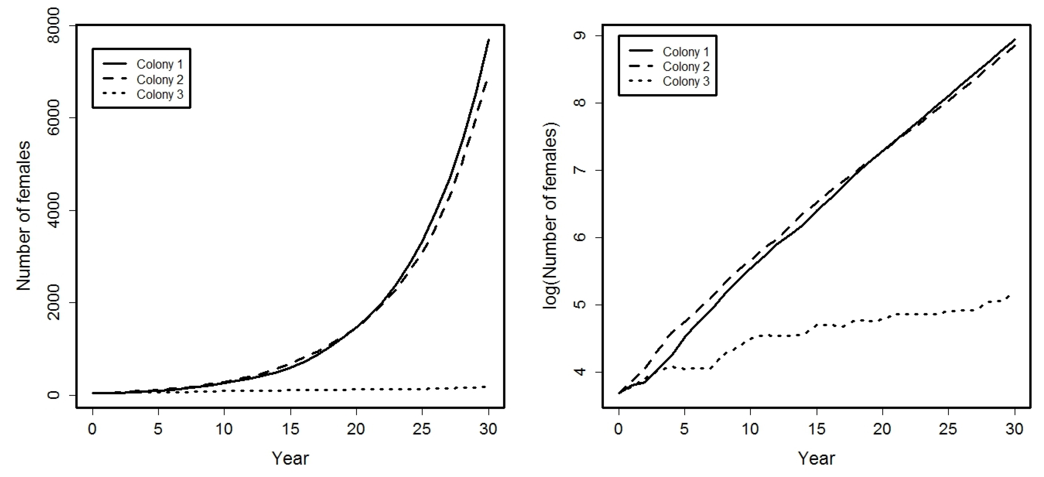
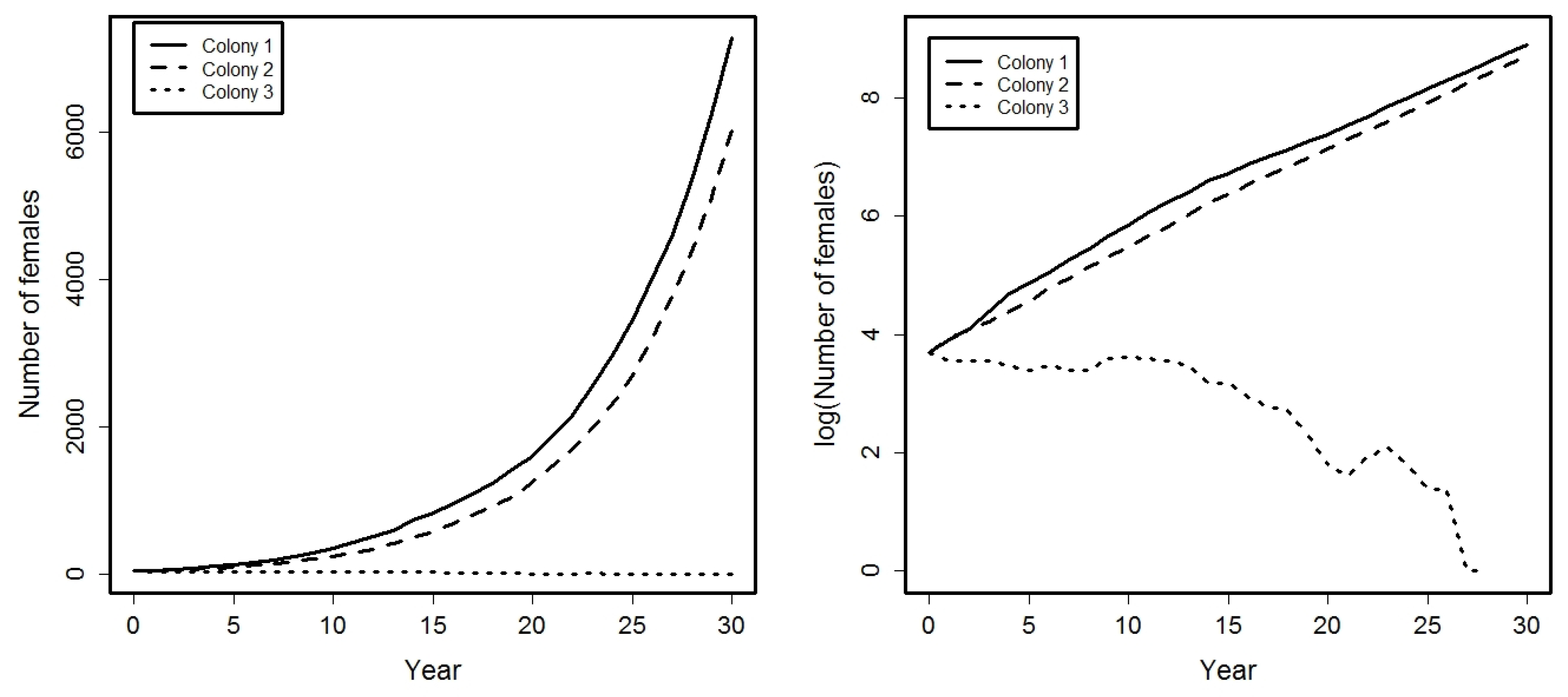
4. Application

We now consider an application of the proposed mathematical model to investigate the demographic dynamics of systems formed by several colonies of large and long-lived raptor species. These type of raptors share several common features, including:

•

The monogamous behavior throughout their life span.

•

The tendency to return to their birthplace or proximity in order to reproduce.

•

The common reproductive behavior. In fact, they have relatively stable populations and tend to produce a low numbers of offspring. The probability of breeding success depends on the age of the female.

•

The viability of their populations depends on the survival rate of the birds. Really, mortality rate in these raptor species during their reproductive life is very low.

For more information about these raptor species see, e.g., [1,22], or [2].

By simplicity, because the stability of the pairs throughout the long life span of these raptor species, the demographic dynamics of their colonies can be described through the female individuals. We will assume a fertile period of d years for a female; a clutch size of one egg and a negligible mortality rate during their fertile period. Suppose that this species is distributed in c geographically separated colonies, being $q_{jh}$ the probability that a female emigrates from colony j to colony h, $j,h\in \{1,\dots ,c\}$.

Notice that, in a first mathematical approximation, the demographic dynamics in such a biological system can be described through the probability model introduced in Section 2, ${\left\{{\mathbf{X}}_{\mathbf{n}}\right\}}_{n=0}^{\infty }$, ${\mathbf{X}}_{\mathbf{n}}={(X_n^{j,k})}_{c\times d}$ where the types in this case are the ages. In this context, $X_n^{j,k}$ denotes the number of k years old females in colony j at year n.

In this biological context, since the clutch size is one egg, the offspring probability distributions are Bernoulli laws. For $k\in \{1,\dots ,d\}$, let $p_k$ be the corresponding success probability for the reproduction of a k years old female (understanding by success to have a female chick that reach adult age). It is derived the mean matrix:

$$\mathbf{M}=\left(\begin{array}{ccccc}{p}_1\hfill & 1& 0& \dots & 0\\ p_2\hfill & 0& 1& \dots & 0\\ ⋮\hfill & ⋮& ⋮& & ⋮\\ p_{d-1}\hfill & 0& 0& \dots & 1\\ p_d\hfill & 0& 0& \dots & 0\end{array}\right)$$

By way of illustration, consider $c=3$ colonies. Though the fertile period of these species is much longer, in order to simplify the example, consider also $d=4$. Finally, assume that:

• Success probabilities at different ages for the females are: $p_1=0.4$, $p_2=0.5$, $p_3=0.3$, $p_4=0.2$.
• A small percentage of females from colonies 1 and 2 emigrate among them: $q_{12}=q_{21}=0.01$.
• Females from colony 3 can emigrate to colonies 1 or 2, being: $q_{31}=q_{32}=0.05$

In this case, we deduce that:

$$\mathbf{M}=\left(\begin{array}{cccc}0.4\hfill & 1& 0& 0\\ 0.5\hfill & 0& 1& 0\\ 0.3\hfill & 0& 0& 1\\ 0.2\hfill & 0& 0& 0\end{array}\right)\mathbf{Q}=\left(\begin{array}{ccc}0.99\hfill & 0.01\hfill & 0\hfill \\ 0.01\hfill & 0.99\hfill & 0\hfill \\ 0.05\hfill & 0.05\hfill & 0.9\hfill \end{array}\right)$$

It can be verified that $\mathbf{M}$ has as Perron-Frobeniüs eigenvalue $\rho =1.17$ and $\mathbf{Q}$ is a reducible matrix.

Also, taking into account (10),

$$\mathbf{Q}=\left(\begin{array}{cc}{\mathbf{Q}}_{\mathbf{11}}& \mathbf{0}\\ {\mathbf{Q}}_{\mathbf{21}}& {\mathbf{Q}}_{\mathbf{22}}\end{array}\right)$$

where:

$${\mathbf{Q}}_{\mathbf{11}}=\left(\begin{array}{cc}0.99\hfill & 0.01\hfill \\ 0.01\hfill & 0.99\hfill \end{array}\right),{\mathbf{Q}}_{\mathbf{21}}=\left(\begin{array}{cc}0.05& 0.05\end{array}\right),{\mathbf{Q}}_{\mathbf{22}}=0.9$$

Thus, it is deduced as eigenvalue of ${\mathbf{Q}}_{\mathbf{22}}$, the value $\lambda =0.9$.

By using the language and environment for statistical computing and graphic R, see [23], initially taking:

$${\mathbf{X}}_{\mathbf{0}}=\left(\begin{array}{cccc}10& 10& 10& 10\\ 10& 10& 10& 10\\ 10& 10& 10& 10\end{array}\right)$$

we simulated a sequence of data from the mathematical model during a period of 30 years.

See Figure 1 where, in left graphic, is showed the evolution of the total number of females in each colony, i.e., ${\displaystyle \sum _{k=1}^4}{X}_n^{j,k}$, $j=1,2,3$, and in the right graphic, the logarithms of those values. Note that, in the left graphic, is observed a faster growth rate in colonies 1 and 2. In fact, right graphic shows a growth rate $\rho =1.17$ at these two colonies, and a growth rate $\lambda \rho =1.053$ at the colony 3.

If the proportion of immigrants towards other colonies increases, “source” colonies can become extinct whereas “receptor” colonies keep growing at the same rate. This fact can be shown by modifying the matrix $\mathbf{Q}$ of the previous example. In fact, if we set

$$q_{31}=q_{32}=0.1q_{33}=0.8$$

then $\rho =1.17$ and $\lambda \rho =0.936$, so colony 3 will become eventually extinct. This can be observed in Figure 2. Right graphic shows clearly how the growth rate at colonies 1 and 2 is $\rho =1.17$, but the graphic of logarithms for colony 3 reach the value 0 at the year 28 and then can not be computed for the subsequent years due to the extinction of the population.

5. Conclusions

This paper proposes a new class of stochastic models to describe the demographic dynamics of complex biological systems formed by various populations in which several types of individuals live, and immigration-emigration phenomena among the involved populations are allowed. The novelty we introduce is that these migratory phenomena take place among several observed populations. Thus, we know from where immigrants come and to where emigrants go. The introduced models are mathematically described through a sequence of random matrices in which rows and columns represent the various populations and the several types of individuals, respectively. By considering a methodology based on multitype branching process theory, several probabilistic properties are established and some limit results are derived. The results obtained have interest in biology and ecology, especially in studies about population dynamics of species.

An open problem for research, is to study results on statistical inference about the more informative parameters involved in the probability model. In particular, it is of great theoretical and practical interest to determine appropriate estimators for the elements of the matrices $\mathbf{M}$ and $\mathbf{Q}$. To this end, some estimation procedures based on Bayesian analysis, such as Approximated Bayesian Computation (ABC) methods or Markov Chain Monte Carlo (MCMC) algorithm, will be useful tools.

References

- Margalida, A.; Colomer, M.A.; Oro, D.; Arlettaz, R.; Donázar, J.A. Assesing the impact of removal scenarios on population viability of a threatened long-lived avian scavenger. Sci. Rep. 2015, 5, 16962. [Google Scholar] [CrossRef] [PubMed]
- Tauler, H.; Real, J.; Hernández-Matías, A.; Aymerich, P.; Baucells, J.; Martorell, C.; Santandreu, J. Identifying key demographic parameters for the viability of a growing population of the endangered Egyptian Vulture Neophron Pernopterus. Bird Conserv. Int. 2015, 25, 246–439. [Google Scholar] [CrossRef]
- Faddy, M.J. Stochastic compartmental models as approximations to more general stochastic systems with the general stochastic epidemic as an example. Adv. Appl. Prob. 1977, 9, 448–461. [Google Scholar] [CrossRef]
- Matis, J.H.; Wehrly, T.E. Stochastic models of compartmental systems. Biometrics 1979, 35, 199–220. [Google Scholar] [CrossRef]
- Asmussen, S.; Hering, H. Branching Processes; Birkhauser Boston, Inc.: Boston, MA, USA, 1983. [Google Scholar]
- Athreya, K.B.; Ney, P.E. Branching Processes; Springer: New York, NY, USA, 1972. [Google Scholar]
- Haccou, P.; Jagers, P.; Vatutin, V. Branching Processes: Variation, Growth and Extinction of Populations; Cambridge University Press: Cambridge, UK, 2005. [Google Scholar]
- Mode, C.J. Multitype Branching Processes. Theory and Applications; American Elsevier Publishing Co., Inc.: New York, NY, USA, 1971. [Google Scholar]
- Quine, M.P. The multi-type Galton-Watson process with immigration. J. Appl. Prob. 1970, 7, 411–422. [Google Scholar] [CrossRef]
- Yakovlev, A.Y.; Yanev, N.M. Branching stochastic processes with immigration in analysis of renewing cell populations. Math. Biosci. 2006, 203, 37–63. [Google Scholar] [CrossRef] [PubMed]
- Yakovlev, A.Y.; Yanev, N.M. Limiting distributions for multitype branching processes. Stoch. Anal. Appl. 2010, 28, 1040–1060. [Google Scholar] [CrossRef] [PubMed]
- Crump, K.S.; Gillespie, J.H. The dispersion of a neutral allele considered as a branching process. J. Appl. Prob. 1976, 13, 208–218. [Google Scholar] [CrossRef]
- Pollak, E. Survival probabilities for some multitype branching processes in genetics. J. Math. Biol. 1992, 30, 583–596. [Google Scholar] [CrossRef]
- Durhan, S.D. An optimal branching migration process. J. Appl. Prob. 1975, 12, 569–573. [Google Scholar] [CrossRef]
- Dawson, D.A.; Greven, A. State dependent multitype spatial branching processes and their longtime behavior. Electron. J. Prob. 2003, 8, 1–93. [Google Scholar]
- Fairweather, D.W.; Shimi, I.N. A Multi-type branching process with immigration and random environment. Math. Biosci. 1972, 13, 299–324. [Google Scholar] [CrossRef]
- Vatutin, V.A. Multitype branching processes with immigration in random environment and polling systems. Siberian Adv. Math. 2011, 21, 42–72. [Google Scholar] [CrossRef]
- Horn, R.A.; Johnson, C.R. Topic in Matrix Analysis; Cambridge University Press: Cambridge, UK, 1994. [Google Scholar]
- Kesten, H.; Stigum, B.P. A limit theorem for multidimensional Galton-Watson processes. Ann. Math. Statist. 1966, 37, 1211–1223. [Google Scholar] [CrossRef]
- Johnson, D. Substochastic Matrix Spectral Radius. Version: 2014-02-07. Available online: https://math.stackexchange.com/q/666603 (accessed on 18 December 2020).
- Kesten, H.; Stigum, B.P. Limit theorems for decomposble multi-dimensional Galton-Watson processes. J. Math. Anal. Appl. 1967, 17, 309–338. [Google Scholar] [CrossRef]
- Newton, I. Population Ecology of Raptors; T and AD Poyser Ltd.: London, UK, 1979. [Google Scholar]
- R Development Core Team. A Language and Environment for Statistical Computing. R Foundation for Statistical Computing. 2009. Available online: http://www.r-project.org (accessed on 18 December 2020).
Publisher’s Note: MDPI stays neutral with regard to jurisdictional claims in published maps and institutional affiliations. |
© 2021 by the authors. Licensee MDPI, Basel, Switzerland. This article is an open access article distributed under the terms and conditions of the Creative Commons Attribution (CC BY) license (http://creativecommons.org/licenses/by/4.0/).
Share and Cite
Molina-Fernández, M.; Mota-Medina, M. Demographic Dynamics in Multitype Populations with Migrations. Mathematics 2021, 9, 246. https://doi.org/10.3390/math9030246
Molina-Fernández M, Mota-Medina M. Demographic Dynamics in Multitype Populations with Migrations. Mathematics. 2021; 9(3):246. https://doi.org/10.3390/math9030246
Chicago/Turabian StyleMolina-Fernández, Manuel, and Manuel Mota-Medina. 2021. "Demographic Dynamics in Multitype Populations with Migrations" Mathematics 9, no. 3: 246. https://doi.org/10.3390/math9030246
APA StyleMolina-Fernández, M., & Mota-Medina, M. (2021). Demographic Dynamics in Multitype Populations with Migrations. Mathematics, 9(3), 246. https://doi.org/10.3390/math9030246