Assessing Efficiency of Public Poverty Policies in UE-28 with Linguistic Variables and Fuzzy Correlation Measures

Abstract

The present study analyzes the efficiency of social expenditure by EU-28 countries within the period 2014–2018 to reduce poverty. The data are provided by programs European Union Statistics on Income and Living Conditions (EU-SILC) and European System of Integrated Social Protection Statistics (ESSPROS) of Eurostat. We first calculate the Debreu–Farrell (DF) productivity measure similarly to our previous work, published in 2020, for each EU-28 country and rank these poverty policies (PPPs) on the basis of that efficiency index. We also quantify the intensity of the relationship between efficiency and the proportion that each item of social expending suppose within the overall. When evaluating public policies within a given number of years, we have available a longitudinal set of crisp observations (usually annual) for each embedded variable and country. The observed value of variables for any country for the whole period 2014–2018 is quantified as fuzzy numbers (FNs) that are built up by aggregating crisp annual observations on those variables within that period. To rank the efficiency of PPPs, we use the concept of the expected value of an FN. To assess the relation between DF index and the relative effort done in each type of social expense, we interpret Pearson’s correlation as a linguistic variable and also use Pearson’s correlation index between FNs proposed by D.H. Hong in 2006.

1. Introduction

This paper assesses public poverty policies (PPPs) in European Union by considering not only attained a diminution of poverty, which obviously is directly linked with social expenditure (SE), but also the productivity of this expenditure. Likewise, we quantify the relationship of every kind of social expenditure (health and sickness benefits, pensions benefits, family and children benefits, …) with the efficiency of overall SE.

There are many papers on the productivity of public policies from the point of view of fiscal systems [1,2,3], but also from the perspective of nonmonetary social benefits, such as health and education [4,5,6]. The productivity of SE to reduce inequality and poverty indexes have also been investigated in for EU-27 countries (EU-28 less Croatia) [7]; within OECD countries [8]; in EU-15 countries [9] and within EU-28 [10,11,12]. Our analysis shows a new perspective on this topic since we analyze a different period, and moreover, we use fuzzy set theory tools to analyze data.

The key question we address here is the relationship between SE, on one hand, and poverty rates on the other in EU-28. It is well known that there is an inverse relation of SE with poverty and inequality indexes [13,14]. However, ref. [15] showed that despite there is a great negative correlation of SE and poverty levels in EU-28 states, it cannot be concluded that increases in SE lead directly to reductions in poverty. Therefore, ref. [15] suggests that more efforts in social benefits suppose unequal results of poverty policies. Hence, convergence in SE does not imply converging in poverty levels. This fact comes clear in the case of Mediterranean countries as, e.g., Spain where a growth of social expenses could end up absorbed by middle-income households instead lower-income ones due to Mathew effect [16]. Indeed, ref. [17] point out that whereas tax systems and in-cash benefits could generate a diminution of income inequality indexes, they may also produce undesired consequences. It is well known that pensions for the elderly people have a small redistributive effect.

Although family and housing benefits are more progressive than pensions, they have a limited impact since they do not suppose a great proportion of SE. On the other hand, ref. [18] indicates that the results of unemployment policies objected to the Lisbon strategy. That paper outlines that unemployment expenses have not had expected results, and also redistribution programs have not been effective enough in poverty elimination. Likewise, several papers found that the benefits of social assistance policies have not a great effect in many countries [19,20,21,22,23]. Hence, we feel justified assessing productivity of SE on poverty diminutions within EU-28 countries. It could lead us to understand why several countries, after making a similar budgetary effort in social policies, obtain different results in poverty reduction due to the unequal productivity of their social programs.

Our analysis on EU-28 PPPs is done within 2014–2018 by using annual data from the Eurostat programs: European Union Statistics on Income and Living Conditions (EU-SILC) and European System of Integrated Social Protection Statistics (ESSPROS). To assess the results of social policies within a period of several years, a usual practice consists of taking the average value of annual observations as variable observations [8,10,12] or, alternatively, limiting the analysis to a concrete year [7,12]. Clearly, those procedures suppose using limited information. This drawback leads us to propose modeling observations on variables in a period of multiple years by means of fuzzy numbers (FNs). Fuzzy data analysis will allow using all the information in the sample and, in addition, structuring the value of observations in such a way that we may obtain results with an intuitive interpretation. With fuzzy data on evaluated PPPs, we perform two analyses. First, we rank EU-28 countries taking into account the productivity of their PPP. To do it we calculate the fuzzy Debreu–Farrell index for each country and face a problem of FN ordering. Second, we calculate and evaluate the correlation of PPP efficiency with the way SE has been split into items as health expenditure, pensions payments, … by using fuzzy tools.

The motivations of our research and its novelty can be summarized as follows:

• Periodic assessment of public policies is a must for their improvement. That explains the existence of a wide literature on social policy evaluation, which has been summarized in above paragraphs. Our analysis complement these papers by showing a different perspective on this topic since we cover a different period and in some cases we use a different sample of countries and database. Likewise, we also use a novel (in this kind of analysis) mathematical instruments. Likewise, our results are compared with those from precedent literature.
• The methodology proposed to deal with the variability in longitudinal data supposes a novelty in the field of public policy evaluation. To the best of our knowledge in this field, there is a scarcity of papers that model uncertainty in data by using soft computing tools as fuzzy sets. In most of the studies on this topic, when an observation is given by a set of crisp results, these are reduced to a real number (e.g., the arithmetical mean) to model the observation. Hence, subsequent analysis is done ignoring actual data uncertainty. The use of fuzzy numbers lets modeling and structuring observed uncertainty and also provides a developed mathematical core that allows handling these data linked with their uncertainty in similar way to we do with real numbers.
• The literature on productivity measurement under fuzziness is built up by adapting conventional data envelopment analysis to fuzzy mathematics, and then so-called fuzzy data envelopment analysis (FDEA) methods reach. Our paper also uses a fuzzy efficient frontier to evaluate productivity, but it is built over the basis of the Debreu–Farrell index that is fitted with a regression method. This way to fit efficient frontier is very common in economics (see [24]) but supposes a novel approach from fuzzy sets literature perspective.

The following section describes the mathematical instruments from fuzzy set theory used in this paper. Methodological aspects of our article: variables, database and methodology that lead to assess the efficiency of SE in poverty reduction are exposed in the third section. In the fourth section, we establish a hierarchy of PPPs in EU-28 by using the concept of the expected value of an FN. Likewise, we evaluate the influence of the composition of SE over the efficiency of PPPs. This last issue is done with the concept of fuzzy correlation and modeling Pearson’s correlation coefficient (PCC) as a fuzzy linguistic variable. The last section presents the principal conclusions from our paper.

2. Concepts of Fuzzy Set Mathematics

2.1. Fuzzy Numbers

A fuzzy number (FN) is a fuzzy set $\tilde{A}$ defined over the set of real numbers, and it is a fundamental concept of FST for representing uncertain quantities. Let us symbolize as ${\mu }_{\tilde{A}}(x)$ the membership function of a fuzzy set $\tilde{A}$. Hence, $\tilde{A}$ is also a FN if it is normal, i.e., $\underset{x\in X }{\max }{\mu }_{\tilde{A}}(x)=1$, and convex, that is, its α-cuts are closed and bounded intervals. Hence, it can be represented as confidence intervals $A_{}=\left[\underset{\_}{A}\left(\alpha \right),\overline{A}\left(\alpha \right)\right]$, where $\underset{\_}{A}\left(\alpha \right)$ ($\overline{A}\left(\alpha \right)$) increases (decreases) monotonously respect the membership degree $\alpha \in \left[0,1\right]$. A FN $\tilde{A}$ is a fuzzy quantity that matches “more or less” the real number A, such that ${\mu }_{\tilde{A}}A)=1$. This paper uses triangular fuzzy numbers (TFNs), that are symbolized as $\tilde{A}=\left(A,l_A,r_A\right)$. Hence, A is the core, and it is the most reliable value: ${\mu }_{\tilde{A}}(A)=1$. Likewise, $l_A,r_A\ge 0$ are the left and right radius and measure the variability of $\tilde{A}$ respect A. Membership function and α-cuts of a FN are:

$${\mu }_{\tilde{A}}(x)=\{\begin{array}{cc}\frac{x-A+l_A}{l_A}& A-l_A<x\le A\\ \frac{A+r_A-x}{r_A}& A<x\le A+r_A\\ 0& \mathrm{otherwise}\end{array}$$

(1a)

$$A_{}=\left[\underset{\_}{A}\left(\alpha \right),\overline{A}\left(\alpha \right)\right]=\left[A-l_A\left(1-\alpha \right),A+r_A\left(1-\alpha \right)\right]$$

(1b)

The hypothesis of a triangular shape for uncertain variables is commonplace in papers on practical applications of FNs. We are aware that this hypothesis may suppose simplifying the complexity of available information. However, we feel that this drawback is balanced by several benefits:

• TFNs are well-adapted to how humans think about imprecise quantities. For example, a prediction as “I expect that for the next two years the GPD growth rate will be 1.5% and deviations no greater than 0.05%” may be quantified in a very natural way as (0.015, 0.005, 0.005). Notice that it is not needed to be a fuzzy set practitioner to interpret and understand the information provided by that FN;
• When the information about a variable is vague and imprecise, as that in this paper, representing the information as simple as possible is desirable, and the linear shape of TFNs meets that requirement;
• TFNs are easier to handle arithmetically than other more complex shapes. From a soft-computing perspective, they provide a good balance between precision on one hand and computational effort and interpretability of results on the other. This fact explains the great deal of literature about approximating triangular shapes to non-TFNs.

In some cases, it will be useful to transform a fuzzy number $\tilde{A}$ into a crisp equivalent. For example, when we are ranking alternatives from their scores in a variable that are done by FNs. Fuzzy literature provides a great deal of ordering methods (see [25]). In this paper, we will use the concept of the expected value of an FN in [26]. Let be an FN $\tilde{A}$ and a parameter $\lambda \in \left[0,1\right]$ that quantifies the evaluator’s optimism grade. The expected value of $\tilde{A}$ for a given λ is:

$$EV(\tilde{A};\lambda )=\left(1-\lambda \right)\underset{0}{\overset{1}{{\displaystyle \int }}}\underset{\_}{A}\left(\alpha \right)d\alpha +\lambda \underset{0}{\overset{1}{{\displaystyle \int }}}\overline{A}\left(\alpha \right)d\alpha$$

(1c)

Hence, for a TFN:

$$EV(\tilde{A};\lambda )=A-\frac{l_A}{2}\left(1-\lambda \right)+\frac{r_A}{2}$$

(1d)

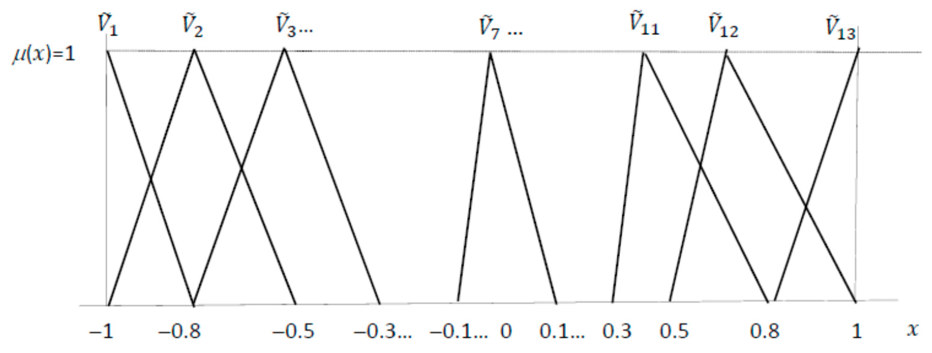
2.2. Modeling the Value of the Pearson Correlation Coefficient as a Linguistic Variable

Linguistic variables are variables whose values are sentences from natural or artificial languages named linguistic labels [27]. They are built up by segmenting a universal set in a set of FNs where each one represents a linguistic label. For example, the variable coefficient of correlation has a reference set [−1, 1] and may be partitioned in several linguistic labels as, e.g., “no correlation”, “low(−)”, “medium(−)”, “high(−)”…}. Hence, “no correlation” may be quantified with the TFN (0, 0.005, 0.005).

Let be a linguistic variable V with a reference set $\left[V_{min}, V_{max}\right]$. It is built up by granulating the reference set into J levels (i.e., J fuzzy numbers), j = 1, 2, …, J, which in this paper are assumed to be TFNs. Then, by considering $V_{min}=V_1<V_2<V_3<\dots <V_{J-1}<V_J=V_{max}$ we obtain:

$$\begin{gathered} \{{\tilde{V}}_{k_1}=\left(V_1,0,V_2-V_1\right); {\tilde{V}}_j=\left(V_j,V_j-V_{j-1},V_{j+1}-V_j\right), j=2,3,\dots ,J-1; \\ {\tilde{V}}_J=\left(V_J,V_J-V_{J-1},0\right)\}. \end{gathered}$$

(2)

Notice that it is accomplished that ${{\displaystyle \sum }}_j{\mu }_{{\tilde{V}}_j}\left(x\right)=1$ for any crisp value $x$∈$\left[V_{min},V_{max}\right].$

The association of a given kind of social expense with the efficiency of PPPs is done by means of a correlation index. As far as decision-making is concerned, it is usual to interpret the value of the correlation coefficient qualitatively by means of linguistic labels as “high (+) correlation” or “weak (−) correlation” that may depend on the context.

Table 1. Interpretation of the Pearson’s and Spearman correlation coefficients.

Correlation Coefficient		Dancey and Reidy (Psychology)	Quinnipiac University (Politics)	Chan (Medicine)
−1	1	Perfect	Perfect	Perfect
−0.9	0.9	Strong	Very Strong	Very Strong
−0.8	0.8	Strong	Very Strong	Very Strong
−0.7	0.7	Strong	Very Strong	Moderate
−0.6	0.6	Moderate	Strong	Moderate
−0.5	0.5	Moderate	Strong	Fair
−0.4	0.4	Moderate	Strong	Fair
−0.3	0.3	Weak	Moderate	Fair
−0.2	0.2	Weak	Weak	Poor
−0,1	0.1	Weak	Negligible	Poor
0	0	Zero	None	None

Source: [28], Akoglu, H. (2018). User’s guide to correlation coefficients. Turkish Journal of Emergency Medicine, 18(3), 91–93.

shows three scales exposed in [27] that are used in psychology, political science and medicine.

By applying (2) on the scale by the Department of Politics at Quinnipiac University in Figure 1, we built up the fuzzy linguistic variable “correlation coefficient” used in this paper to qualitatively interpret the correlation. It is shown in

Table 2. Fuzzy linguistic variable “coefficient of correlation” built up from de Quinnipiac University scale.

Negative Correlation		Positive Correlation
Fuzzy Number	Linguistic Label	Fuzzy Number	Linguistic Label
${\tilde{V}}_1=\left(-1,0,0.2\right)$	Perfect (−)	${\tilde{V}}_{13}=\left(1,0.2,0\right)$	Perfect (+)
${\tilde{V}}_2=\left(-0.8,0.2,0.3\right)$	Very strong (−)	${\tilde{V}}_{12}=\left(0.8,0.3,0.2\right)$	Very strong (+)
${\tilde{V}}_3=\left(-0.5,0.3,0.2\right)$	Strong (−)	${\tilde{V}}_{11}=\left(0.5,0.2,0.3\right)$	Strong (+)
${\tilde{V}}_4=\left(-0.3,0.2,0.1\right)$	Moderate (−)	${\tilde{V}}_{10}=\left(0.3,0.1,0.2\right)$	Moderate (+)
${\tilde{V}}_5=\left(-0.2,0.1,0.1\right)$	Weak (−)	${\tilde{V}}_9=\left(0.2,0.1,0.1\right)$	Weak (+)
${\tilde{V}}_6=\left(-0.1,0.1,0.1\right)$	Negligible (−)	${\tilde{V}}_8=\left(0.1,0.1,0.1\right)$	Negligible (+)
${\tilde{V}}_7=\left(0,0.1,0.1\right)$	No correlation	${\tilde{V}}_7=\left(0,0.1,0.1\right)$	No correlation

Source: own elaboration by using Table 1 in [28], Akoglu, H. (2018). User’s guide to correlation coefficients. Turkish Journal of Emergency Medicine, 18(3), 91–93.

.

2.3. Aggregating Crisp Observations by Means of a Triangular Fuzzy Number

In this paper, we capture the uncertainty in data by using FNs. We are aware that Soft Computing Science provides several tools apart from fuzzy sets to represent uncertain data: rough sets, gray sets, intuitionistic and neutrosophic sets… Using FNs instead other alternatives presents pros and cons. In any case we feel that using TFN in our analysis is suitable for the following reasons:

• Tools as intuitionistic fuzzy sets (IFSs) or neutrosophic fuzzy sets (NFSs) provide an analytical framework to quantify uncertainty more precisely than FNs. Therefore, they are able to capture more nuances from data and its imprecision. For example, NFS state for any element not only a truth membership degree but also an indeterminacy and a falsity degree. However, their estimation implies a greater cost since the number of parameters to fit for each uncertain observation is three times that number than in the case of FNs. On the other hand, gray numbers (GNs) provide a simpler representation of uncertain quantities than FNs. To define a GN is enough to fit its kernel and a grayness measure. Hence, in several circumstances GNs may oversimplify information. For example, GNs suppose a symmetrical structure for a uncertain quantity when perhaps available information does not suggest so. TFNs balances capturing much of the uncertainty in available information (less than, e.g., NFS, but more than GNs), but with a smooth shape (less than GNs, but more than NFSs).
• In many circumstances, rough sets also could provide accurate quantification of uncertainty. However, as we will explain below, our problem is more linked to vagueness in observations than with their indiscernibility.
• Our analysis needs implementing arithmetical operations with uncertain variables, ranking them and evaluating Pearson’s correlation with uncertain observations. Fuzzy sets literature has developed these questions widely, and so the use of TFNs allows making these analyses similar to real numbers. Likewise, fuzzy arithmetic allows results conserving the triangular shape as well as the uncertainty within data throughout calculations.

Cheng in [29] proposes a method that allows transforming a set of crisp observations on a given variable in an FN. Let us symbolizing as {a₁, a₂, …, a_n} the set of crisp observations and $\tilde{A}=\left(A,l_A,r_A\right)$ the TFN than will embed these observations. To fit $\tilde{A}$ the following steps must be followed:

Step 1. Calculate the distance between ith and jth value as $d_{ij}=\left|a_i-a_j\right|$. Of course, $d_{ii}=0, d_{ij}=d_{ji}$. Hence, we can build up a distance matrix $\mathit{D}={\left[d_{ij}\right]}_{n\times n}$.

Step 2. Calculate the mean distance of ith opinion the other n − 1 as:

$${\overline{d}}_i=\frac{{{\displaystyle \sum }}_{i=1}^n{d}_{ij}}{n-1}$$

(3a)

Hence, ${\overline{d}}_i$ measures the distance of ith opinion to the center of gravity of the opinion pool. Of course, the weight of the value a_i to determine A is decreasing respect to ${\overline{d}}_i$.

Step 3. Find the matrix $\mathit{P}={\left[p_{ij}\right]}_{n\times n}$ that indicates the importance of ith opinion over the jth to fix A by doing:

$$p_{ij}=\frac{{\overline{d}}_j}{{\overline{d}}_i}$$

(3b)

Moreover, so, $p_{ii}=1$ and $p_{ij}=\frac{1}{ p_{ji}}$. Notice that P is obtained from a comparison of distances and so, it ensures its consistency, i.e., that there is a coherent judgment in specifying the pairwise comparison of score importance.

Step 4. Fit coefficients w_i, i = 1, 2, …, n, which measure the degree of importance of ith observation to fit $\tilde{A}$, in such a way $0\le w_i\le 1,$ i = 1, 2, …, n. These weights are adjusted by taking into account the relative degree of importance of ith observation respect jth, j = 1, 2, …, n (3b). Following [29], if we symbolize as w the vector of weights nx1, Pw = nw, where n is an eigenvalue of P and w an eigenvector. Likewise, given that it must accomplished that ${{\displaystyle \sum }}_{i=1}^n{w}_i=1$, the weights are solved from (3b) by doing:

$$w_i=\frac{1}{{{\displaystyle \sum }}_{j=1}^n{p}_{ji}}$$

(3c)

Hence, ref. [29] indicates that the consistency of P lead to:

$$p_{ij}=\frac{w_i}{w_j}$$

(3d)

Step 5. Calculate the center of $\tilde{A}$ as:

$$A={\displaystyle \sum }_{i=1}^n{w}_i{a}_i$$

(3e)

Step 6. Estimate so-called mean deviation $(\sigma )$ of the FN $\tilde{A}$ as a first step to adjusting their spreads. Hence, ref. [29] defines the mean deviation of a FN as $\sigma =\frac{{{\displaystyle \int }}_{A-l_A}^{A+r_A}\left|x-A\right|{\mu }_{\tilde{A}}x)dx}{{{\displaystyle \int }}_{A-l_A}^{A+r_A}{\mu }_{\tilde{A}}x)dx}$ and then for a TFN $\sigma =\frac{l_A^2+r_A^2}{3\left(l_A+r_A\right)}$ By using the rate of the left spread respect to the right $\eta =\frac{l_A}{r_A}$:

$$l_A=\frac{3 \left(1+\eta \right)\eta \sigma }{1+{\eta }^2} \mathrm{and} r_A=\frac{3 \left(1+\eta \right)\sigma }{1+{\eta }^2}$$

(3f)

Notice that $\sigma$ and $\eta$ are, in fact, unknown parameters because they are built up from $l_A$ and $r_A$. Hence, ref. [29] proposes the following approximation for $\sigma , \widehat{\sigma }$:

$$\widehat{\sigma }={{\displaystyle \sum }}_{i=1}^n{w}_i\left|A-a_i\right|$$

(3g)

Step 7. Find the estimate of $\eta , \widehat{\eta }$. By defining as $a^l=\frac{{{\displaystyle \sum }}_{\begin{array}{c}i=1\\ a_i<A\end{array}}^n{w}_i{a}_i}{{{\displaystyle \sum }}_{\begin{array}{c}i=1\\ a_i<A\end{array}}^n{w}_i}$ and $a^r=\frac{{{\displaystyle \sum }}_{\begin{array}{c}i=1\\ a_i>A\end{array}}^n{w}_i{a}_i}{{{\displaystyle \sum }}_{\begin{array}{c}i=1\\ a_i>A\end{array}}^n{w}_i}$, $\widehat{\eta }$ is:

$$\widehat{\eta }=\frac{A-a^l}{a^r-A}$$

(3h)

Step 8. Find l_A and r_A by doing

$$l_A=\frac{3 \left(1+\widehat{\eta }\right)\widehat{\eta }\widehat{\sigma }}{1+{\widehat{\eta }}^2} \mathrm{and} r_A=\frac{3 \left(1+\widehat{\eta }\right)\widehat{\sigma }}{1+{\widehat{\eta }}^2}$$

(3i)

Numerical Application 1

Table 3. Annual social expenses (over GPD) by Belgium in the period 2014–2018.

Year	2014	2015	2016	2017	2018
SER	30	29.8	29.2	28.8	28.8

Source: own elaboration from data provided by EU-SILC (2008–2018) and ESSPROS (2008–2017).

shows the values provided by Eurostat within 2014–2018 of the social expenses over GPD, SER = SE/GPD for Belgium. Let us fitting that variable for the quinquennium as a TFN $\widetilde{SER}=\left(SER,l_{SER},r_{SER}\right)$ by using (3a)–(3i).

The matrix of distances between observations is exposed in

Table 4. Matrix of distances to build up the fuzzy number “Belgian SER within 2014–2018”.

	2014	2015	2016	2017	2018
2014	0	0.2	0.8	1.2	1.2
2015	0.2	0	0.6	1	1
2016	0.8	0.6	0	0.4	0.4
2017	1.2	1	0.4	0	0
2018	1.2	1	0.4	0	0

Source: own elaboration from data provided by EU-SILC (2008–2018) and ESSPROS (2008–2017).

, and the relative importance of each annual value of SER in the final TFN is provided in

Table 5. Relative importance of social expenses over GPD (SER) in each year in the triangular fuzzy numbers (TFN) “Belgian SER in 2014–2018”.

	2014	2015	2016	2017	2018
2014	1	0.824	1.294	0.765	0.765
2015	1.214	1	1.571	0.929	0.929
2016	0.773	0.636	1	0.591	0.591
2017	1.308	1.077	1.692	1	1
2018	1.308	1.077	1.692	1	1

Source: own elaboration from data provided by EU-SILC (2008–2018) and ESSPROS (2008–2017).

.

Then, the vector of weights is: $w=\left(0.178, 0.217, 0.138, 0.233, 0.233\right)$ and, therefore SER = 29.286. To fit the spreads, $l_{SER}$ and $r_{SER}$ we find that $\widehat{\sigma }=0.478$, $SE{R}^l=28.89$ and $SE{R}^r=29.89$. Hence, $\widehat{\eta }=\frac{29.286-28.89}{29.89-29.286}=0.654$, $l_{SER}=\frac{3 \left(1+0.654\right)·0.654·0.478}{1+{0.654}^2}$ = 1.085 and $r_{SER}=\frac{3 \left(1+0.654\right)·0.478}{1+{0.654}^2}$ = 1.660. Hence, annual SER by Belgium for 2014–2018 is fitted as $\widetilde{SER}=\left(29.286\%,1.085\%,1.660\%\right)$.

Notice that quantifying Belgian SER as the TFN $\widetilde{SER}=\left(29.286\%,1.085\%,1.660\%\right)$ is very suited to the intuition that comes after a visual inspection of Table 3 “Belgium SER has been around 29% within 2014–2018”. Of course, more sophisticated representations of uncertainty as IFSs or NFSs can capture a greater amount of information. However, the cost of fitting these kind of sets is much greater and not very reliable with the information available for our analysis (identical to that in Table 3 for Belgium SER). On the other hand, if information came from an extended and structured questionnaire submitted to experts, surely NFSs will provide a better representation of that information than FNs.

Belgium SER in Table 3 admits a gray number representation. Following the exposition in [30] and taking into account that SER in Table 3 is within the interval [28.8, 30] since is the discrete set {28.8, 28.8, 29.2, 29.8, 30}, the kernel of SER is $S\widehat{E}R=$ (28.8 + 28.8 + … +30)/5 = 29.32. Grayness degree can be estimated by taking into account that SER for any country must be within [0, 100] and so its value is (30 − 28.8)/100 = 0.012. By using notation in [30], SER is 29.32_(0.012). Notice that this parameterization is simpler than $\widetilde{SER}=\left(29.286\%,1.085\%,1.660\%\right)$, but on the other hand, the TFN captures the asymmetric distribution of values around the gravity center of the data that GN does not.

Due to the kind of data that we will use in our analysis, we feel that using TFN parameterization from [29] provides an adequate compromise between applying the principle of parsimony in vagueness modeling and avoiding unnecessary loss of information.

2.4. Correlation Coefficients for Fuzzy Data

Pearson’s correlation coefficient (PCC) is a real-valued function in ℜ²ⁿ of the pairwise observations over the variables X and Y$:$ $\left\{\left(x_1,y_1\right);\left(x_2,y_2\right);\dots ;\left(x_n,y_n\right)\right\}$. Hence, PCC between X and Y is estimated as:

$$cor{r}_{X.Y}=f\left(x_1,\dots ,x_n;y_1,\dots ,y_n\right)=\frac{{{\displaystyle \sum }}_{i=1}^n\left(x_i-\frac{{{\displaystyle \sum }}_{i=1}^n{x}_i}{n}\right)\left(y_i-\frac{{{\displaystyle \sum }}_{i=1}^n{y}_i}{n}\right)}{\sqrt{{{\displaystyle \sum }}_{i=1}^n{\left(x_i-\frac{{{\displaystyle \sum }}_{i=1}^n{x}_i}{n}\right)}^2{{\displaystyle \sum }}_{i=1}^n{\left(y_i-\frac{{{\displaystyle \sum }}_{i=1}^n{y}_i}{n}\right)}^2}}$$

(4a)

i.e., $cor{r}_{X.Y}$ is a function $f\left(x_1,\dots ,x_n;y_1,\dots ,y_n\right)$. Hence, if pairwise observations are given by FNs $\{({\tilde{X}}_1,{\tilde{Y}}_1); ({\tilde{X}}_2,{\tilde{Y}}_2);\dots ;({\tilde{X}}_n,{\tilde{Y}}_n)\}$, $cor{r}_{X.Y}$ induce a FN:

$${\widetilde{corr}}_{X.Y}=f({\tilde{X}}_1,\dots ,{\tilde{X}}_n;{\tilde{Y}}_1,\dots ,{\tilde{Y}}_n)=\frac{{{\displaystyle \sum }}_{i=1}^n\left({\tilde{X}}_i-\frac{{{\displaystyle \sum }}_{i=1}^n{\tilde{X}}_i}{n}\right)\left({\tilde{Y}}_i-\frac{{{\displaystyle \sum }}_{i=1}^n{\tilde{Y}}_i}{n}\right)}{\sqrt{{{\displaystyle \sum }}_{i=1}^n{\left({\tilde{X}}_i-\frac{{{\displaystyle \sum }}_{i=1}^n{\tilde{X}}_i}{n}\right)}^2}\sqrt{{{\displaystyle \sum }}_{i=1}^n{\left({\tilde{Y}}_i-\frac{{{\displaystyle \sum }}_{i=1}^n{\tilde{Y}}_i}{n}\right)}^2}}$$

(4b)

Fuzzy literature has proposed two ways to estimate PCC when the observations are done by FNs (FPCC). The first approach to FPCC, ref. [31], applies Zadeh’s extension principle to (4b). So:

$${\mu }_{{\widetilde{corr}}_{X,Y}}(z)=\underset{z=f\left(x_1,\dots ,x_n;y_1,\dots ,y_n\right)}{max}min[{\mu }_{{\tilde{X}}_1}{x}_1),\dots .,{\mu }_{{\tilde{X}}_n}{x}_n);{\mu }_{{\tilde{Y}}_1}{y}_1),\dots .,{\mu }_{{\tilde{Y}}_n}{y}_n)]$$

(5a)

Notice that it is often difficult computing the membership function of ${\widetilde{corr}}_{X.Y}$. Following [32], it may be easier computing $cor{r}_{X,Y}{}_{\alpha }$ such as:

$$\begin{array}{cc}\hfill cor{r}_{X,Y}{}_{\alpha }=& \left[\underset{\_}{cor{r}_{X,Y}}\left(\alpha \right),\overline{cor{r}_{X,Y}}\left(\alpha \right)\right]\hfill \\ & \hspace{1em}\hspace{1em}=\{z=f\left(x_1,\dots ,x_n;y_1,\dots ,y_n\right)|x_j\in \left[{\underset{\_}{X}}_j\left(\alpha \right),{\overline{X}}_j\left(\alpha \right)\right],y_j\hfill \\ & \hspace{1em}\hspace{1em}\in \left[{\underset{\_}{Y}}_j\left(\alpha \right),{\overline{Y}}_j\left(\alpha \right)\right], j=1,2,\dots ,n\}\hfill \end{array}$$

(5b)

Hence, in (5b) $\underset{\_}{cor{r}_{X,Y}}\left(\alpha \right)$ ($\overline{cor{r}_{X,Y}}\left(\alpha \right)$) are the global minimum (maximum) of f(·) within the rectangular domain in (5b).

$$\underset{\_}{cor{r}_{X,Y}}\left(\alpha \right)=\underset{j,k}{min}\left\{f\left(V_j\right),f\left(E_k\right)\right\} \mathrm{and} \overline{cor{r}_{X,Y}}\left(\alpha \right)=\underset{j,k}{max}\left\{f\left(V_j\right),f\left(E_k\right)\right\}$$

(5c)

Being the vector in ℜ²ⁿ $V_j$, j = 1, 2, …, 2²ⁿ a vertex of (5b), $f\left(E_k\right)$ k = 1, 2, …, K an extreme point of the function and $E_k$ an interior point of (5b). Hence, to find the lower (upper) extreme of α-cuts, a nonlinear minimizing (maximizing) mathematical program must be solved.

The second approach to fit fuzzy correlation uses the weakest T-norm (Tw -norm) in [33] instead of the min operator. So:

$$T_W\left(a,b\right)=\{\begin{array}{c}a \mathrm{if} b=1\\ b \mathrm{if} a=1\\ 0 \mathrm{otherwise}\end{array}$$

(6a)

where $T_W\left(a,b\right)\le min\left(a,b\right)$.

Since the max-operator is still the T-conorm to apply the use of the norm (6a), suppose we reformulate the membership function of the correlation between X and Y as:

$${\mu }_{{\widetilde{corr}}_{X,Y}}(z)=\underset{z=f\left(x_1,\dots ,x_n;y_1,\dots ,y_n\right)}{max}{T}_W[{\mu }_{{\tilde{X}}_1}{x}_1),\dots .,{\mu }_{{\tilde{X}}_n}{x}_n);{\mu }_{{\tilde{Y}}_1}{y}_1),\dots .,{\mu }_{{\tilde{Y}}_n}{y}_n)]$$

(6b)

Tw-norm lets obtaining less uncertain results than min-norm. Likewise, Tw-norm allows an easier computation of (4b) when the observations are LR fuzzy numbers [34] since ${\widetilde{corr}}_{X,Y}$ will conserve L-R shape. In the particular case of TFNs, the calculation of ${\widetilde{corr}}_{X.Y}$. is developed in [35]. In [33] following arithmetical rules to handle arithmetically two TFNs $\tilde{A}=\left(A,l_A,r_A\right)$ and $\tilde{B}=\left(B,l_B,r_B\right)$ are stated:

$$\tilde{A}+\tilde{B}=\left(A,l_A,r_A\right)+\left(B,l_B,r_B\right)=\left(A+B,max(l_A,l_B\right),max\left( r_A,r_B\right))$$

(6c)

$$\tilde{A}-\tilde{B}=\left(A,l_A,r_A\right)-\left(B,l_B,r_B\right)=\left(A-B,max(l_A,r_B\right),\left( r_A,l_B\right))$$

(6d)

$$\lambda \tilde{A}=\lambda \left(A,l_A,r_A\right)=\{\begin{array}{c}\left(\lambda A,\lambda l_A,\lambda r_A\right), \lambda >0\\ \left(\lambda A,-\lambda r_A,\lambda l_A\right), \lambda \le 0\end{array}$$

(6e)

$$\sqrt{\tilde{A}}\approx \left(\sqrt{A},\frac{l_A}{\sqrt{A}},\frac{r_A}{\sqrt{A}}\right), A-l_A>0$$

(6f)

$$\frac{1}{\tilde{A}}\approx \left(\frac{1}{A},\frac{r_A}{A^2},\frac{l_A}{A^2}\right), A-l_A>0$$

(6g)

$$\begin{array}{cc}\hfill \tilde{A}·\tilde{B}& =\left(A,l_A,r_A\right)·\left(B,l_B,r_B\right)=\hfill \\ & =\{\begin{array}{c}\left(A·B,max\left(A·l_B,B·l_A\right),max\left(A·r_B,B·r_A\right)\right) if A,B\ge 0\\ \left(A·B,-max\left(A·l_B,B·l_A\right),-max\left(A·r_B,B·r_A\right)\right) if A,B\le 0\\ \left(A·B,max\left(-A·r_B,B·l_A\right),max\left(-A·l_B,B·r_A\right)\right) if A\le 0,B\ge 0\\ \left(A·B,-max\left(A·l_B,-B·r_A\right),-max\left(A·r_B,-B·l_A\right)\right) if A,B\le 0\end{array}\hfill \end{array}$$

(6h)

$$\begin{array}{c}\frac{\tilde{A}}{\tilde{B}}=\left(A,l_A,r_A\right)\left(\frac{1}{B},\frac{r_B}{B^2},\frac{l_B}{B^2}\right)\\ =\{\begin{array}{c}\left(A·B,max\left(\frac{A·r_B}{B^2},B·l_A\right),max\left(\frac{A·l_B}{B^2},B·r_A\right)\right) if A,B\ge 0\\ \left(A·B,max\left(-A\frac{A·l_B}{B^2},B·l_A\right),max\left(-\frac{A·r_B}{B^2},B·r_A\right)\right) if A\le 0,B\ge 0\end{array}\\ \mathrm{being} B-l_B>0\end{array}$$

(6i)

Hence, to fit ${\widetilde{corr}}_{X.Y}=\left(cor{r}_{X.Y}, l_{cor{r}_{X.Y}},r_{cor{r}_{X.Y}}\right)$. We must evaluate (4b) with (6c)–(6i).

Of course, FPCC may be interpreted qualitatively by using the linguistic variable defined in Table 2. If min T-norm is used, the compatibility grade of ${\widetilde{corr}}_{X.Y}$ with the jth linguistic label ${\tilde{V}}_j$ $C({\widetilde{corr}}_{X.Y},{\tilde{V}}_j)$ can be found by using the max-min rule as:

$$C({\widetilde{corr}}_{X.Y},{\tilde{V}}_j)=\underset{x}{max} min\left[{\mu }_{{\widetilde{corr}}_{X.Y}}x),{\mu }_{{\tilde{V}}_j}x)\right]$$

(7a)

On the other hand, if Tw-norm is used and so the correlation is calculated by following (6c)–(6h), the compatibility between ${\widetilde{corr}}_{X.Y}$ and ${\tilde{V}}_j$ is measured by using a max-Tw rule:

$$C({\widetilde{corr}}_{X.Y},{\tilde{V}}_k)=\underset{}{max}\left[{\mu }_{{\widetilde{corr}}_{X.Y}}{V}_j),{\mu }_{{\tilde{V}}_j}{corr}_{X.Y})\right]$$

(7b)

In both cases, we can find the closest linguistic label in Table 1 to ${\widetilde{corr}}_{X.Y}$, ${\tilde{V}}_k$, by doing:

$${\tilde{V}}_k=\arg max{\{C({\widetilde{corr}}_{X.Y},{\tilde{V}}_j)\}}_{k=1\le j\le n}$$

Numerical Application 2

We fit for 2014–2018 FPCC between social expenses over GPD (SER) and the percentual diminution of poverty risk index (RRP) in EU-28 countries. Fuzzy observations of these variables are shown in

Table 6. Fuzzy observations on social expenses over GPD, relative reduction of poverty-at risk index and Debreu–Farrell measure in the period 2014–2018.

	${\widetilde{\mathit{S}\mathit{E}\mathit{R}}}_{\mathit{i}}=\left(\mathit{S}\mathit{E}{\mathit{R}}_{\mathit{i}},{\mathit{l}}_{\mathit{S}\mathit{E}{\mathit{R}}_{\mathit{i}}},{\mathit{r}}_{\mathit{S}\mathit{E}{\mathit{R}}_{\mathit{i}}}\right)$			${\widetilde{\mathit{R}\mathit{R}\mathit{P}}}_{\mathit{i}}=\left(\mathit{R}\mathit{R}{\mathit{P}}_{\mathit{i}},{\mathit{l}}_{\mathit{R}\mathit{R}{\mathit{P}}_{\mathit{i}}},{\mathit{r}}_{\mathit{R}\mathit{R}{\mathit{P}}_{\mathit{i}}}\right)$			${\widetilde{\mathit{D}\mathit{F}}}_{\mathit{i}}=\left(\mathit{D}{\mathit{F}}_{\mathit{i}},{\mathit{l}}_{\mathit{D}{\mathit{F}}_{\mathit{i}}},{\mathit{r}}_{\mathit{D}{\mathit{F}}_{\mathit{i}}}\right)$
Country	$\mathit{S}\mathit{E}{\mathit{R}}_{\mathit{i}}$	${\mathit{l}}_{\mathit{S}\mathit{E}{\mathit{R}}_{\mathit{i}}}$	${\mathit{r}}_{\mathit{S}\mathit{E}{\mathit{R}}_{\mathit{i}}}$	$\mathit{R}\mathit{R}{\mathit{P}}_{\mathit{i}}$	${\mathit{l}}_{\mathit{R}\mathit{R}{\mathit{P}}_{\mathit{i}}}$	${\mathit{r}}_{\mathit{R}\mathit{R}{\mathit{P}}_{\mathit{i}}}$	$\mathit{D}{\mathit{F}}_{\mathit{i}}$	${\mathit{l}}_{\mathit{D}{\mathit{F}}_{\mathit{i}}}$	${\mathit{r}}_{\mathit{D}{\mathit{F}}_{\mathit{i}}}$
Belgium	29.29	1.09	1.66	41.43	8.19	5.15	0.590	0.030	0.003
Denmark	32.82	2.10	3.22	51.86	5.74	3.77	0.728	0.046	0.033
Germany	29.52	0.82	0.51	33.36	0.23	0.59	0.538	0.056	0.040
Ireland	15.82	2.38	3.95	53.42	3.61	5.92	1.000	0.000	0.000
Greece	25.67	1.72	0.88	16.13	0.23	2.36	0.295	0.017	0.063
Spain	24.09	1.34	2.36	25.09	3.63	6.03	0.399	0.031	0.028
France	34.22	0.60	0.36	44.15	2.49	0.95	0.607	0.074	0.118
Italy	29.28	0.85	1.29	21.37	1.02	0.09	0.302	0.038	0.031
Luxembourg	22.19	0.74	1.03	40.35	3.39	1.50	0.656	0.039	0.064
Netherlands	29.59	1.00	1.54	42.73	5.62	6.58	0.599	0.037	0.054
Austria	29.66	0.94	0.49	44.28	4.07	2.69	0.623	0.019	0.054
Portugal	25.19	1.65	2.56	24.65	3.30	5.08	0.454	0.020	0.049
Finland	31.24	2.21	1.18	54.51	1.52	4.48	0.774	0.110	0.089
Sweden	28.98	1.04	0.64	45.71	3.08	2.18	0.767	0.052	0.014
UK	26.62	1.01	1.68	42.18	4.67	2.36	0.680	0.060	0.037
Bulgaria	17.39	1.45	1.29	21.12	3.60	6.38	0.400	0.061	0.106
Czechia	18.90	0.51	0.82	41.84	4.38	1.45	0.661	0.049	0.071
Estonia	16.00	0.46	0.91	24.94	4.62	6.02	0.456	0.065	0.019
Croatia	21.76	0.21	0.10	29.59	6.13	7.69	0.485	0.090	0.095
Cyprus	19.39	2.47	1.71	36.53	0.22	2.55	0.637	0.055	0.070
Latvia	14.93	0.22	0.51	20.57	5.13	2.69	0.386	0.099	0.057
Lithuania	15.47	0.58	0.86	23.33	0.36	3.96	0.464	0.007	0.080
Hungary	18.76	1.97	1.36	44.72	4.12	6.88	0.817	0.065	0.079
Malta	16.66	2.22	1.69	30.64	0.49	1.71	0.517	0.072	0.047
Poland	19.79	1.29	1.02	29.95	6.79	8.98	0.497	0.096	0.110
Romania	14.73	0.23	0.41	14.56	3.32	4.90	0.303	0.109	0.079
Slovenia	23.20	2.21	1.43	42.85	1.19	1.99	0.636	0.077	0.108
Slovakia	18.17	0.59	0.39	32.42	5.35	8.34	0.492	0.057	0.088

Source: own elaboration from data provided by EU-SILC (2008–2018) and ESSPROS (2008–2017). Variables SER and RRP are expressed over 100 and DF over 1.

. Likewise, we also fit crisp PCC by considering as observations the core triangular shapes SER and RRP (3e).

The α-cut representation of two FPCCs is given in

Table 7. α-cut representation of [31,34] FPPC between SER and relative reduction of poverty in EU-28 countries within the period 2014–2018.

	Max–Min Correlation		Max-Tw Correlation
α	$\underset{\_}{cor{r}_{X,Y}}\left(\alpha \right)$	$\overline{cor{r}_{X,Y}}\left(\alpha \right)$	$\underset{\_}{cor{r}_{X,Y}}\left(\alpha \right)$	$\overline{cor{r}_{X,Y}}\left(\alpha \right)$
0	−0.0643	0.7635	0.4196	0.4819
0.25	0.0762	0.7040	0.4294	0.4761
0.5	0.2140	0.6332	0.4391	0.4702
0.75	0.3427	0.5511	0.4488	0.4644
1	0.4585	0.4585	0.4585	0.4585

Source: own elaboration from data provided by EU-SILC (2008–2018) and ESSPROS (2008–2017).

. Of course, crisp PCC is simply the 1-cut of both FPCCs, i.e., 0.4585. Hence, FPCC generalizes the results of crisp PCC since this last is the core of FPCCs. Likewise, $\alpha$-cuts of FPCCs can be understood as an structured set of simulations that range from maximum fuzziness scenario (generated by the 0-cut of fuzzy estimates of SER and RRP) to maximum reliability situation (that comes from the cores of the observations on SER and RRP).

FPCC in [31] does not preserve the triangular shape of input data. On the other hand, by using FPCC [34], we obtain ${\widetilde{corr}}_{X.Y}$ = (0.4585, 0.0389, 0.0413).

Table 8. Qualitative interpretation of max-min, max- Tw-conorm and crisp correlation between SER and relative reduction of poverty in EU 28 countries within the period 2014–2018 by using $C({\widetilde{corr}}_{X.Y},{\tilde{V}}_k)$.

Linguistic Label	Max–Min	Max-Tw	Crisp	Linguistic Label	Max–Min	Max-Tw
1 Perfect (−)	0	0	0	8 Negligible (+)	0.42	0	0
2 Very strong (−)	0	0	0	9 Weak (+)	0.58	0	0
3 Strong (−)	0	0	0	10 Moderate (+)	0.78	0.21	0.21
4 Moderate (−)	0	0	0	11 Strong (+)	0.92	0.79	0.79
5 Weak (−)	0.0	0	0	12 Very strong (+)	0.44	0	0
6 Negligible (−)	0.1	0	0	13 Perfect (+)	0	0	0
7 No correlation	0.26	0	0	$argmax[C({\widetilde{corr}}_{X.Y},{\tilde{V}}_j)]$	Strong (+) correlation	Strong (+) correlation	Strong (+) correlation

Source: own elaboration from data provided by EU-SILC (2008–2018) and ESSPROS (2008–2017).

shows that the closest linguistic label for both correlations is “strong (+) relation”. However, max-min correlation is extremely imprecise since embed values from −0.0643 (no correlation) to 0.7635 (very strong (+)), and so it is compatible with 4 linguistic levels in a truth level above 0.5. Those levels vary from “negligible (+) correlation” to “very strong (+) correlation”. On the other hand, the correlation [34] is clearly less uncertain and allows a better balance between maintaining all the information in the sample, which is not made by conventional PCC and providing a useful value to obtain conclusions.

2.5. Literature Revision

Evaluating the productivity of a set of entities (in this case, countries) with a Debreu–Farrell efficient frontier, as we do in this paper, is very common in standard economic literature [24], but not at all fuzzy literature. On the other hand, productivity evaluation has been developed extensively within fuzzy literature by means of fuzzy data envelopment analysis (DEA) methods. Zhou and Xu [36] show that only in year 2018 more than 700 papers on fuzzy DEA were published. Without aim to be extensive, let us point out some applications in Economics and Finance. Wu et al. [37] deal with the evaluation of bank efficiency; [38,39] are devoted with the assessment of sustainability in energy and transportation policies and [40] use fuzzy DEA to examine profits by foreign investment in transition Economies.

Similar problems as we address in this paper have been analyzed fruitfully by using fuzzy multiple criteria decision-making (FMCDM). However, usually these methods need using expert opinions as a input. Our study does not use this information. Fuzzy literature has provided a great deal of methods on this issue by mixing existing tools to represent uncertain quantities (fuzzy sets, hesitant fuzzy sets, IFSs…) with well-known Multiple Criteria Decision-Making schedules (AHP, PROMETHEE, ELECTREE, TOPSIS, …). A panoramic review on this matter can be consulted in [41]. Some applications in areas linked with public decision-making are energy policies [41,42], environmental decisions [43,44], healthcare evaluation [45,46], urbanism [47], public infrastructure management [48,49], assessment transparency by public organisms [50] or general economic policy analysis [51].

Fuzzy Pearson’s correlation coefficient has been used in several areas of Economics and Finance. Hence, ref. [52,53] use FPCC to model interactions between asset return in portfolio management and [31,54,55] apply FPCC in several business administration issues as, e.g., capital budgeting problems. Likewise, ref. [56,57] analyze the relationship between variables embedded in education policy. In [35,58] FPCC is used to evaluate attributes of hotel services. Finally, ref. [59] uses FCCC to state the linkage between price index and exchange rates in China.

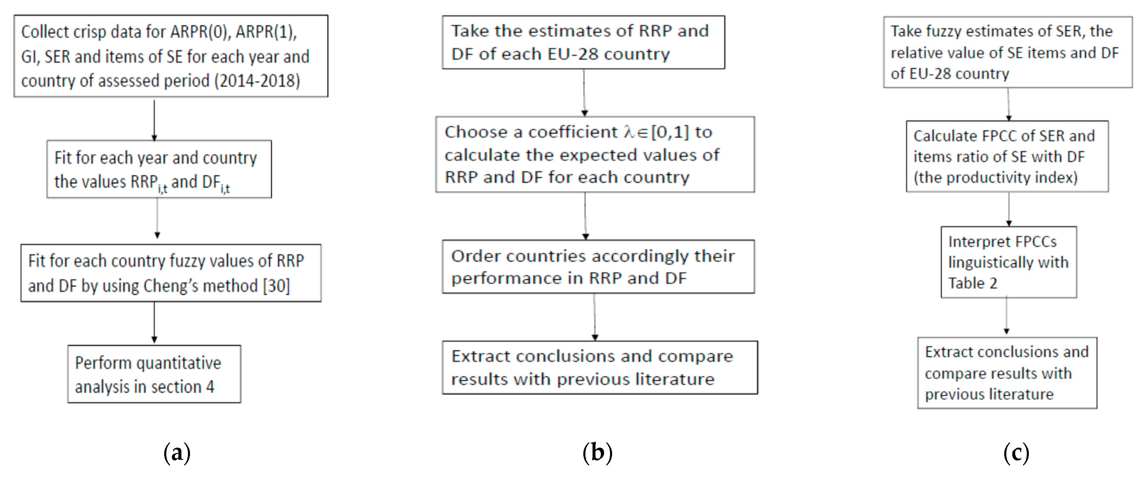
3. Data and Methodology

3.1. Data Description

The data we have used is provided by Eurostat programs EU-SILC and ESSPROS and embeds EU-28 countries in 2018 (i.e., it is included Great Britain). The data have annual periodicity and comprise the period 2014–2018. From the database, we directly obtain observations on the following variables for every country and year. Concretely:

• ARPR(0)_i,t = At-risk-of-poverty rate before social transfers including pensions for the ith country at year t;
• ARPR(1)_i,t = At-risk-of-poverty rate after social transfers for the ith country at year t;
• GI_i,t = Income inequality (measured as the Gini index) before social transfers for the ith country at year t;
• SER_i,t = Ratio social expenses/GDP before social transfers for the ith country at year t.

Likewise, our analysis also needs the observations on the proportion that each kind of social benefit supposes over whole social expending according to EU-SILC classification. These items are defined over the basis of eight protection functions linked with a set of needs [60]:

• Sickness/healthcare benefits (Sick_i,t)—Include, for example, medical assistance or the provision of pharmaceutical products;
• Disability benefits (Dis_i,t)—Pensions, goods and services for disabled persons;
• Old age benefits (Old_i,t)—Basically retirement pensions;
• Survivors’ benefits (Surv_i,t)—An example are survivors’ pensions;
• Family/children benefits (Fam_i,t)—Support programs linked to pregnancy assistance, childbirth, etc.;
• Unemployment benefits (Une_i,t)—Include unemployment in-cash benefits, but also vocational training services provided by public agencies;
• Housing benefits (Hou_i,t)—Interventions and programs from public agencies to help households reaching housing expenses;
• Social exclusion benefits not elsewhere classified (n.e.c.) (SocE_i,t)—A miscellanea of public interventions that may include, e.g., rehabilitation of drug abusers, etc.

From the variables indicated above, we derivate for each country and year the diminution of poverty and the productivity that SE has reached in such diminution. Following [10], we measure poverty reduction in relative terms. Hence, for the ith country at year t we obtain:

$${RRP}_{i,t}=\frac{ARPR{\left(0\right)}_{i,t}-ARPR{\left(1\right)}_{i,t}}{{ARPR\left(0\right)}_{i,t}}, i=1,2,\dots ,28$$

(8)

Hence, RRP_i,t ranks from 0 (and so ARPR(0)_i,t = ARPR(1)_i,t), to 1 (if poverty is completely eliminated).

When analyzing the productivity of SE in reducing poverty risk, we seek to determine to what extent the diminution of poverty (the assessed output) is adequate to the initial situation of poverty and SER (inputs). To measure the efficiency of public spending in achieving poverty reduction for the ith country in a year t we follow [10] that quantifies efficiency by means of a Debreu–Farrell coefficient, DF_i,t. Hence, we consider SE and, more concretely, its quantification by means of its ratio with GPD (SER) as the main input. We also use the GI before transfers as second input variable to reflect the social status of the population before executing the SE. Hence, GI is not strictly an input, but a contextual variable. Likewise, GI is clearly linked to economic context, social and demographical structure and public policy priorities of every state. A greater retired people supposes a larger population that depends on pensions. Likewise, higher unemployment rates imply a greater number of citizens with small (or null) personal income. The method used to evaluate the productivity of PPP in [10] is based on fitting the efficient productive frontier by mixing corrected least-squares method (CLS) and logit regression. Hence, for a year t it is estimated:

$$logit\left(RR{P}_{i.t}\right)={\beta }_{0,t}+{\beta }_{1,t}SE{R}_{i,t}+{\beta }_{2,t}G{I}_{i,t}+{\epsilon }_{i,t}$$

(9)

where the error term accomplishes ${\epsilon }_{i,t}$ ≥ 0, i = 1, 2, …, 28. After adjusting the value of ${\beta }_{0,t},{\beta }_{1,t} \mathrm{and} {\beta }_{2,t}$ with corrected least squares, ${\beta }_{0,t}^F,{\beta }_{1,t}^F,{\beta }_{2,t}^F$, the estimate of the productive frontier value of $RR{P}_{i.t}$, $RR{P}_{i,t}^F$ is:

$$RR{P}_{i,t}^F=\frac{1}{1+exp(-{\beta }_{0,t}^F-{\beta }_{0,t}^F{SER}_{i,t}-{\beta }_{0,t}^F{GI}_{i,t})}$$

(10a)

Hence, Debreu–Farrell efficiency measure for ith country in the year t, $D{F}_{i,t}$, is the ratio between its attained RRP $\left(RR{P}_{i.t}\right)$ in (8) and frontier value of RRP in (10a), $RR{P}_{i,t}^F:$

$$D{F}_{i,t}=\frac{RR{P}_{i.t}}{RR{P}_{i,t}^F}$$

(10b)

where $0\le D{F}_{i,t}\le 1$. Hence, $D{F}_{i,t}=1$ imply full efficiency and $D{F}_{i,t}=0$, complete nonefficiency.

Eurostat database provides the values of the variables related to the social protection benefits and poverty of EU-28 countries with an annual periodicity. Therefore, the variables RRP and DF are calculated with this periodicity. To evaluate the results of social policies within a period of more than one year (e.g., a quinquennium), a usual practice consists of taking for the variables the average of their annual observations [8,10,12]. Other papers reduce the analysis to a concrete year [7,11]. A complete analysis consists of repeating it in every year of the period of interest as it is done in Lefevre et al. (2010). Alternatively, we propose quantifying the variables in a period of multiple years by means of TFNs that are built up from observed longitudinal point values of those variables.

Our analysis is done by using SER, the proportion that each kind of social expense suppose over whole SE, the relative reduction of poverty RRP (8) and Debreu–Farrell efficiency index (10) of all countries throughout 2014–2018. We fit for the ith country the value of any variable “A” (e.g., SER) for the whole period 2014–2018 as an FN ${\tilde{A}}_i=\left(A_i,l_{A_i},r_{A_i}\right)$ i = 1, 2, …, 28. They are fitted from the point observations in each year of the period that we are analyzing, {a₂₀₁₄, a₂₀₁₅, a₂₀₁₆, a₂₀₁₇, a₂₀₁₈} by following the method in Section 2.3. Figure 2a summarizes all the process followed to fit TFNs to the observations on variables embedded in the study. Table 6 shows the fuzzy estimates of SER (${\widetilde{SER}}_i$), RRP (${\widetilde{RRP}}_i$) and efficiency index DF, (${\widetilde{DF}}_i$) in EU-28 countries. Fuzzy values of the proportion that each item of social spending (Sick, Dis, Old, …) suppose in overall SE are in

Table A1. Proportion that 8 items of social benefits suppose in overall social expenditures (percentage).

	Sickness/Healthcare			Disability			Old Age			Survivors			Family/Children			Unemployment			Housing			Social Exclusion
Country	Center	Left	Right	Center	Left	Right	Center	Left	Right	Center	Left	Right	Center	Left	Right	Center	Left	Right	Center	Left	Right	Center	Left	Right
Belgium	27.019	0.097	1.07	8.458	1.18	0.755	38.439	4.508	5.208	6.525	0.306	0.206	7.498	0.177	0.22	5.492	1.221	0.939	1.51	0.017	0.037	2.425	0.543	0.371
Denmark	21.282	1.172	0.708	16.181	0.733	0.197	38.731	0.81	1.333	0.783	0.13	0.257	11.139	0.252	0.156	2.625	0.24	0.408	1.345	0.522	0.289	5.165	0.626	0.386
Germany	35.144	0.089	0.166	8.207	0.56	0.986	32.301	0.113	0.174	6.312	0.314	0.505	11.403	0.182	0.246	4.681	1.027	0.766	2.173	0.041	0.021	0.979	0.401	0.262
Ireland	36.908	3.55	2.537	5.443	0.248	0.41	31.465	0.824	1.301	2.723	0.077	0.022	9.053	0.873	0.61	2.792	0.254	0.164	0.335	0.363	0.204	0.769	0.056	0.085
Greece	19.421	0.883	1.824	4.371	0.086	1.028	55.4	0.986	2.994	10.107	0.418	1.121	4.874	1.626	2.953	10.12	5.252	3.744	3.534	0.673	0.99	1.285	1.358	0.538
Spain	26.683	0.711	1.001	7.174	0.071	0.208	41.002	3.669	2.356	9.84	0.049	0.12	5.368	0.162	0.261	3.736	0.197	0.332	0.054	0.148	0.096	0.999	0.028	0.013
France	28.564	0.39	0.258	6.449	0.048	0.021	40.17	0.02	0.194	5.384	0.192	0.262	7.68	0.229	0.368	8.345	2.059	3.276	0.443	0.045	0.027	3.068	0.239	0.347
Italy	23.132	0.086	0.276	5.713	0.2	0.175	48.987	0.093	0.039	9.492	0.123	0.31	4.1	0.192	0.057	2.895	0.45	1.114	0.106	0.032	0.019	2.728	0.967	0.627
Luxembourg	24.977	0.575	0.855	10.857	0.568	0.856	31.362	2.845	1.614	7.743	0.672	0.457	15.439	0.174	0.25	3.581	1.412	0.963	0.396	0.129	0.081	2.257	0.106	0.064
Netherlands	33.766	1.342	1.998	9.16	0.846	0.081	38.346	0.294	0.196	3.933	0.548	0.34	3.977	0.853	0.486	2.61	1.117	0.766	0.858	0.422	0.357	4.941	0.818	0.293
Austria	25.528	0.546	1.059	6.516	0.426	0.644	44.421	0.186	0.263	5.871	0.365	0.507	9.523	0.15	0.094	4.641	2.304	1.592	1.641	0.196	0.1	1.989	0.292	0.698
Portugal	24.994	2.525	1.759	7.223	0.417	0.293	50.339	0.655	0.994	7.6	0.063	0.154	4.834	0.519	0.347	1.235	0.309	0.472	0.224	0.102	0.146	0.905	0.125	0.073
Finland	23.023	1.057	1.958	9.943	0.814	1.393	40.985	3.512	4.921	2.702	0.083	0.135	10.02	0.319	0.52	2.887	0.122	0.073	0.253	0.066	0.109	2.926	0.15	0.404
Sweden	26.145	0.396	0.685	10.241	0.661	1.302	43.582	0.801	1.188	1.091	0.207	0.315	10.386	0.281	0.394	7.816	2.316	1.193	2.452	0.778	1.093	3.278	1.379	1.034
United Kingdom	32.463	0.775	0.427	6.324	0.762	0.518	42.446	0.469	0.724	0.311	0.023	0.033	9.968	0.399	0.54	3.623	0.238	0.104	1.498	0.126	0.177	2.318	0.217	0.162
Bulgaria	28.053	1.645	2.532	7.451	0.271	0.44	43.932	1.386	0.951	5.422	0.128	0.167	10.631	0.573	0.264	8.919	6.385	4.871	0.847	0.046	0.068	1.47	0.517	0.282
Czechia	32.281	2.131	1.574	6.464	0.323	0.399	43.783	0.265	0.373	3.312	0.277	0.377	8.811	0.102	0.343	3.005	0.309	0.215	0	0	0	1.332	0.705	0.503
Estonia	29.601	1.311	0.65	11.503	0.281	0.525	42.104	2.793	4.276	0.352	0.065	0.098	12.929	2.022	1.362	3.545	0.413	0.579	1.969	0.111	0.046	0.554	0.083	0.202
Croatia	32.987	1.502	0.516	11.046	1.498	2.377	33.636	0.464	0.179	8.981	0.809	1.221	8.79	0.304	0.57	6.132	0.219	0.11	2.55	0.176	0.097	1.498	0.704	0.453
Cyprus	17.912	2.278	1.598	4.116	1.522	1.059	48.577	1.015	1.585	7.227	0.11	0.081	6.816	0.28	0.496	5.723	0.423	0.679	0.13	0.049	0.026	6.696	1.184	0.696
Latvia	25.047	1.514	2.511	9.071	0.255	0.322	48.129	2.182	3.453	1.258	0.049	0.084	10.755	0.88	0.078	6.681	3.123	2.625	1.83	0.351	0.212	0.741	0.099	0.174
Lithuania	30.315	2.63	1.584	9.3	0.336	0.117	43.377	3.021	4.716	2.718	0.54	0.348	8.026	1.122	2.132	4.318	0.693	0.451	0.534	0.19	0.26	2.005	0.616	1.132
Hungary	27.18	2.944	1.617	6.364	1.235	1.77	44.766	0.64	1.243	5.518	0.859	0.604	11.949	0.114	0.174	5.949	1.157	1.669	1.585	0.501	0.342	0.565	0.109	0.169
Malta	33.927	2.388	1.649	3.647	0.235	0.34	43.323	1.827	1.161	8.274	0.107	0.19	5.963	1.002	1.743	1.785	0.198	0.341	1.894	1.02	1.514	1.302	0.318	0.558
Poland	22.952	0.65	1.455	7.553	1.217	0.845	47.42	4.599	1.978	9.328	1.08	1.8	11.102	8.806	5.041	5.668	0.101	0.245	0.379	0.149	0.082	0.623	0.158	0.219
Romania	27.116	0.806	1.307	6.907	1.606	1.212	50.284	0.694	0.065	4.467	0.319	0.526	9.513	2.525	1.649	3.954	1.788	2.842	0	0	0	1.056	0.466	0.248
Slovenia	33.015	3.168	1.867	5.309	1.698	1.314	41.847	0.631	0.486	6.169	0.9	0.614	7.963	0.667	1.008	0.591	0.396	0.615	0.103	0.039	0.05	3.103	0.157	0.253
Slovakia	31.739	0.838	2.036	8.809	0.282	0.189	40.67	0.362	0.477	4.996	0.238	0.356	9.088	0.374	0.14	2.598	0.432	0.664	0.107	0.016	0.005	1.56	0.54	0.808

Source: own elaboration from data provided by EU-SILC (2008–2018) and ESSPROS (2008–2017).

of annex.

3.2. Methodology

We first rank UE28 states by considering the efficiency of their PPP. To make this assessment, we defuzzify the values of DF with (1d) and state their hierarchy. Likewise, we relate our results with those in [7,10]. The flowchart of this analysis is depicted in Figure 2b.

The second analysis tries to determine the sign of the relation between the eight items that [60] differentiates in social expending and the efficiency of PPP. Figure 2c shows how we have implemented this assessment on European PPPs. As it is stated in [16] and also checked in [7,8,10], despite the clear negative linkage between SER and poverty indexes in EU-28, it cannot be concluded that a poverty reduction is reached automatically by increasing SER. Hence, we first measure the intensity of the relation between the effort in social policies (i.e., SER) with the results in reducing poverty (RRP) and with PPP efficiency measured by DF. Subsequently we investigate why two different countries with a similar SER will obtain different reductions of poverty indexes. Following [7,10] we perform this analysis with the FPCC of the proportion that each kind of social benefit supposes in overall social expenditure. Concretely we use FPCC in [34] (Equations (4b) and (6a)–(6i)) instead max-min fuzzy correlation due to the reasons exposed above. We have used the fuzzy version of PPC instead other correlation measure as, e.g., Spearman correlation by two reasons. First, we pretend comparing our results with those in [7,10] that evaluate the PPPs of the same set of countries, and they use Pearson’s correlation coefficient. To allow our results to be fully comparable, the same correlation measure must be used. Likewise, calculating Spearman correlation requires an early defuzzification of triangular observations in order to rank them, e.g., by calculating their expected value. Subsequently Spearman correlation index is a real valued number since that comes from applying a conventional PPC on the crisp rank of variables. Therefore, the fuzzy uncertainty of data is waived in that correlation measure.

Within EU-28, we can differentiate two types of countries whose history and political evolution from II World War to the end of the 20th century XX has been notably different. One on hand we have EU-15 countries, basically Western Europe countries, which are part of European Union from 20th-century. On the other hand, we find former communist republics plus Cyprus and Malta that belonged progressively in European Union during the 21st century.

Table 9. Mean values of SER, poverty risk index (RRP) and Debreu–Farrell index (DF) in EU-28, EU-15 and non-EU-15 in the period 2014–2018.

	${\widetilde{\mathit{S}\mathit{E}\mathit{R}}}^{\mathit{M}}$			${\widetilde{\mathit{R}\mathit{R}\mathit{P}}}^{\mathit{M}}$			${\widetilde{\mathit{D}\mathit{F}}}^{\mathit{M}}$
	$\mathit{S}\mathit{E}{\mathit{R}}^{\mathit{M}}$	${\mathit{l}}_{\mathit{S}\mathit{E}{\mathit{R}}^{\mathit{M}}}$	${\mathit{r}}_{\mathit{S}\mathit{E}{\mathit{R}}^{\mathit{M}}}$	$\mathit{R}\mathit{R}{\mathit{P}}^{\mathit{M}}$	${\mathit{l}}_{\mathit{R}\mathit{R}{\mathit{P}}^{\mathit{M}}}$	${\mathit{r}}_{\mathit{R}\mathit{R}{\mathit{P}}^{\mathit{M}}}$	$\mathit{D}{\mathit{F}}^{\mathit{M}}$	${\mathit{l}}_{\mathit{D}{\mathit{F}}^{\mathit{M}}}$	${\mathit{r}}_{\mathit{D}{\mathit{F}}^{\mathit{M}}}$
EU-28	23.190	0.088	0.141	34.796	0.292	0.321	0.563	0.004	0.004
Non EU-15	18.089	0.190	0.131	30.236	0.522	0.691	0.519	0.008	0.008
EU-15	27.612	0.165	0.263	38.748	0.546	0.598	0.601	0.007	0.008

Source: own elaboration from data provided by EU-SILC (2008–2018) and ESSPROS (2008–2017). Variables SER and RRP are expressed over 100 and E over 1.

shows the mean value of ${\widetilde{SE}}_i$, ${\widetilde{RRP}}_i$ and ${\widetilde{DF}}_i$, i = 1, 2, …, 28 in EU-28, but also, separately, the average value of EU-15 countries and non-EU-15 states. Those mean values have been obtained by using Max-Tw norm convolution in such a way that for a variable A, the mean value ${\tilde{A}}^M$ is:

$${\tilde{A}}^M=\left(A^M,l_{A^M},r_{A^M}\right)=\left(\frac{{{\displaystyle \sum }}_{i=1}^n{A}_i}{n},\frac{\underset{i}{\max }{l}_{A_i}}{n},\frac{\underset{i}{\max }{r}_{A_i}}{n}\right)$$

(11)

In Table 9 it can be checked that the mean value of EU-15 and non-EU-15 in SER, RRP and efficiency of PPP is completely different. EU-15 countries present a mean value of SER 10 points above non-EU-15 countries. Likewise, Table 9 shows that whereas EU-15 countries rarely have a value for SER below 25%, non-EU-15 states with SER greater than 20% are an exception. Consequently, the mean reduction of poverty in EU-15 countries is clearly above non-EU-15 states. It is also remarkable that the mean DF is notably greater in EU-15 countries than in non-EU-15 countries.

4. Results

4.1. Ranking Public Poverty Policies by the EU-28 States

The results of PPPs efficiency are given in

Table 10a. Ranking social policy in UE-28 countries on the basis of the expected value of RRP and DF in Table A2 for several values of λ.

Criteria	Relative Reduction of Poverty (RRP)				Debreu–Farrell Ratio (DF)
Country	λ = 1	λ = 0.5	λ = 0	V–F	λ = 1	λ = 0.5	λ = 0	V–F
Belgium	12	13	13	13	14	14	13	19
Denmark	3	3	3	5	5	5	5	7
Germany	16	15	15	14	15	15	15	10
Ireland	2	2	2	10	1	1	1	3
Greece	27	27	27	21	26	26	26	21
Spain	20	20	20	25	24	24	23	28
France	7	6	5	4	12	12	14	14
Italy	25	25	24	19	27	27	27	27
Luxembourg	13	12	12	11	7	8	7	5
Netherlands	9	9	9	3	13	13	12	8
Austria	6	7	8	8	11	9	9	16
Portugal	22	21	22	17	21	21	20	18
Finland	1	1	1	6	3	4	4	11
Sweden	5	4	4	12	4	3	3	6
United Kingdom	10	10	10	15	8	6	6	17
Bulgaria	24	24	25	27	23	23	24	26
Czechia	11	11	11	1	6	7	7	1
Estonia	21	23	23	26	22	22	22	23
Croatia	19	19	19	22	20	20	21	22
Cyprus	14	14	14	20	10	9	10	25
Latvia	26	26	26	28	25	25	25	24
Lithuania	23	22	21	23	19	18	18	15
Hungary	4	5	6	2	2	2	2	2
Malta	17	17	16	18	17	16	16	20
Poland	18	18	18	16	18	19	19	13
Romania	28	28	28	24	28	28	28	12
Slovenia	8	8	7	9	9	11	11	9
Slovakia	15	16	17	7	16	17	17	4

Source: own elaboration from data provided by EU-SILC (2008–2018) and ESSPROS (2008–2017). V–F stands for the rank in [10] within the period 2007–2015.

,

Table 10b. Spearman correlations between the expected values of RRP and/or DF for several values of the index of optimism λ.

	RRP (λ = 1)	RRP (λ = 0.5)	RRP (λ = 0)	RRP (V–F)	DF (λ = 1)	DF (λ = 0.5)	DF (λ = 0)	DF (V–F)
RRP (λ = 1)	1
RRP (λ = 0.5)	0.996	1
RRP (λ = 0)	0.991	0.997	1
RRP (V–F)	0.830	0.831	0.824	1
DF (λ = 1)	0.943	0.947	0.941	0.784	1
DF (λ = 0.5)	0.939	0.944	0.937	0.757	0.994	1
DF (λ = 0)	0.935	0.939	0.932	0.761	0.992	0.997	1
DF (V–F)	0.642	0.652	0.642	0.795	0.718	0.680	0.692	1

Source: own elaboration from data provided by EU-SILC (2008–2018) and ESSPROS (2008–2017). Note: As V–F, we symbolize the value of RRP and DF obtained by Valls-Fonayet et al. (2020) within the period 2007–2015.

and

Table A2. Expected value of fuzzy RRP (over 100) and E (over 1) for several values of the index of λ.

	Relative Reduction of Poverty (RRP)			Debreu–Farrell Ratio (DF)
Country	λ = 1	λ = 0.5	λ = 0	λ = 1	λ = 0.5	λ = 0
Belgium	39.91	38.62	37.34	0.577	0.576	0.575
Denmark	50.88	49.93	48.99	0.722	0.713	0.705
Germany	33.54	33.39	33.25	0.53	0.52	0.51
Ireland	54.58	53.10	51.62	1	1	1
Greece	17.20	16.61	16.02	0.318	0.302	0.287
Spain	26.29	24.78	23.28	0.398	0.391	0.384
France	43.38	43.14	42.91	0.629	0.600	0.570
Italy	20.91	20.88	20.86	0.299	0.291	0.283
Luxembourg	39.41	39.03	38.66	0.669	0.653	0.637
Netherlands	43.21	41.57	39.92	0.608	0.594	0.581
Austria	43.59	42.92	42.25	0.641	0.627	0.614
Portugal	25.54	24.27	23.00	0.469	0.456	0.444
Finland	55.99	54.87	53.75	0.764	0.741	0.719
Sweden	45.26	44.72	44.17	0.748	0.745	0.741
United Kingdom	41.03	40.44	39.85	0.669	0.659	0.650
Bulgaria	22.51	20.92	19.32	0.423	0.396	0.370
Czechia	40.38	40.01	39.65	0.672	0.654	0.637
Estonia	25.64	24.14	22.63	0.433	0.428	0.424
Croatia	30.37	28.45	26.53	0.488	0.464	0.440
Cyprus	37.70	37.06	36.42	0.645	0.627	0.610
Latvia	19.35	18.68	18.01	0.365	0.351	0.337
Lithuania	25.13	24.14	23.15	0.501	0.481	0.461
Hungary	46.10	44.38	42.66	0.824	0.804	0.785
Malta	31.25	30.82	30.40	0.505	0.493	0.481
Poland	31.05	28.80	26.56	0.504	0.477	0.449
Romania	15.35	14.13	12.90	0.288	0.268	0.249
Slovenia	43.25	42.75	42.26	0.652	0.625	0.598
Slovakia	33.92	31.83	29.75	0.508	0.486	0.464

Source: own elaboration from data provided by EU-SILC (2008–2018) and ESSPROS (2008–2017).

of the annex A. It can be checked in Table 10b that all hierarchies in RRP and DF index present a correlation close to 1. This fact does not depend on the coefficient λ used to defuzzify ${\widetilde{RRP}}_i$ and ${\widetilde{DF}}_i$, i = 1, 2, …, 28. Hence, by applying fuzzy linguistic interpretation of correlation proposed in Section 2.2, we can conclude that all the expected values of RRP and DF present a perfect(+) correlation.

The results that we have obtained are similar to those in [7,9,12]. Better performances are attained by Anglo-Saxon welfare states (Ireland and Great Britain), Scandinavian welfare states (Finland, Sweden and Denmark) and some Visegrad pact countries like Hungary and Czechia. The less efficient PPPs are those from the Mediterranean welfare states (Italy, Greece, Spain) and some Mediterranean and Baltic former communist republics as Romania, Bulgaria, Latvia or Estonia. In intermediate positions, we find continental welfare states (as, e.g., France, Belgium, etc.) and a heterogeneous set of non-UE-15 as, e.g., Cyprus, Malta or Slovakia. Table 10b shows that the hierarchies in Valls-Fonayet et al. in [10] and those in our paper present a Spearman correlation coefficient that Table 2 labels as very strong (+).

4.2. Fuzzy Assessment of the Relation between Social Expense Effort and Efficiency in Poverty Reduction

Table 11. Correlations of SER with RRP and DF efficiency index.

	EU-28			Non-EU-15 Countries			EU-15 Countries
	$\mathit{c}\mathit{o}\mathit{r}{\mathit{r}}_{\mathit{X}.\mathit{Y}}$	${\mathit{l}}_{\mathit{c}\mathit{o}\mathit{r}{\mathit{r}}_{\mathit{X}.\mathit{Y}}}$	${\mathit{r}}_{\mathit{c}\mathit{o}\mathit{r}{\mathit{r}}_{\mathit{X}.\mathit{Y}}}$	$\mathit{c}\mathit{o}\mathit{r}{\mathit{r}}_{\mathit{X}.\mathit{Y}}$	${\mathit{l}}_{\mathit{c}\mathit{o}\mathit{r}{\mathit{r}}_{\mathit{X}.\mathit{Y}}}$	${\mathit{r}}_{\mathit{c}\mathit{o}\mathit{r}{\mathit{r}}_{\mathit{X}.\mathit{Y}}}$	$\mathit{c}\mathit{o}\mathit{r}{\mathit{r}}_{\mathit{X}.\mathit{Y}}$	${\mathit{l}}_{\mathit{c}\mathit{o}\mathit{r}{\mathit{r}}_{\mathit{X}.\mathit{Y}}}$	${\mathit{r}}_{\mathit{c}\mathit{o}\mathit{r}{\mathit{r}}_{\mathit{X}.\mathit{Y}}}$
RRP	0.459	0.039	0.023	0.715	0.100	0.078	0.125	0.075	0.091
DF	0.194	0.062	0.038	0.569	0.086	0.078	−0.204	0.131	0.079

Source: own elaboration from data provided by EU-SILC (2008–2018) and ESSPROS (2008–2017).

and

Table 12. Value of the compatibility indexes (7b) of the correlations between SER with RRP and DF and the labels of linguistic variable “correlation coefficient”.

	EU-28		Non-EU-15		EU-15
Linguistic Label	SER vs. RRP	SER vs. DF	SER vs. RRP	SER vs. DF	SER vs. RRP	SER vs. DF
Perfect (−)	0	0	0	0	0	0
Very Strong (−)	0	0	0	0	0	0
Strong (−)	0	0	0	0	0	0
Moderate (−)	0	0	0	0	0	0.267
Weak (−)	0	0	0	0	0	0.970
Negligible (−)	0	0	0	0	0	0.207
No corr	0	0	0	0	0	0
Negligible (+)	0	0.065	0	0	0.750	0
Weak (+)	0	0.935	0	0	0.250	0
Moderate (+)	0.207	0	0	0	0	0
Strong (+)	0.793	0	0.283	0.771	0	0
Very Strong (+)	0	0	0.717	0.229	0	0
Perfect (+)	0	0	0	0	0	0
argmax	Strong (+)	Weak (+)	Very strong (+)	Strong (+)	Negligible (+)	Weak (−)

Source: own elaboration from data provided by EU-SILC (2008–2018) and ESSPROS (2008–2017).

show the relation of the volume of social expenses with the reduction of poverty and its efficiency. As we expected, in the whole EU-28, the relation between SER and RRP is positive (strong (+)). However, the behavior of that relation is completely different in EU-15 and non-EU 15. In non-EU 15 countries it is very strong (+), i.e., there is a direct relation between the volume of social expenses and poverty reduction. On the other hand, in EU-15 countries that relation is negligible. Hence, this result is in accordance with the statement in [16] that showed that despite there is a strong negative correlation between SER and poverty rates in several European countries, it cannot be concluded that increases in SER lead directly to reductions in poverty.

Likewise, in whole EU-28 countries, the relation between the volume of social expenditure and its efficiency is weak (+). Again, the relation between these variables in non-EU-15 countries and EU-15 states is completely different. In EU-15 countries, that relation is weak (−), whereas in non-EU-15 countries is strong (+). Notice that the value of SER in non-EU-15 countries is substantially lower than in EU-15 countries. Therefore, its marginal productivity of SER is clearly positive when social expenses are relatively low, and so a greater diminution of poverty comes fair from increasing SE. However, when a critical level of SER is reached, the relationship between increases in SER and diminutions in RRP is not so direct. This fact motivates a detailed analysis of the influence of the social expenditure composition over the value of DF reached by every PPP.

From

Table 13. Value of the correlations between DF and the proportion that each kind of social expense suppose in overall SER.

	EU-28			Non-EU-15			EU-15
Item	$\mathit{c}\mathit{o}\mathit{r}{\mathit{r}}_{\mathit{X}.\mathit{Y}}$	${\mathit{l}}_{\mathit{c}\mathit{o}\mathit{r}{\mathit{r}}_{\mathit{X}.\mathit{Y}}}$	${\mathit{r}}_{\mathit{c}\mathit{o}\mathit{r}{\mathit{r}}_{\mathit{X}.\mathit{Y}}}$	$\mathit{c}\mathit{o}\mathit{r}{\mathit{r}}_{\mathit{X}.\mathit{Y}}$	${\mathit{l}}_{\mathit{c}\mathit{o}\mathit{r}{\mathit{r}}_{\mathit{X}.\mathit{Y}}}$	${\mathit{r}}_{\mathit{c}\mathit{o}\mathit{r}{\mathit{r}}_{\mathit{X}.\mathit{Y}}}$	$\mathit{c}\mathit{o}\mathit{r}{\mathit{r}}_{\mathit{X}.\mathit{Y}}$	${\mathit{l}}_{\mathit{c}\mathit{o}\mathit{r}{\mathit{r}}_{\mathit{X}.\mathit{Y}}}$	${\mathit{r}}_{\mathit{c}\mathit{o}\mathit{r}{\mathit{r}}_{\mathit{X}.\mathit{Y}}}$
Sick	0.234	0.038	0.034	−0.008	0.078	0.115	0.443	0.053	0.041
Dis	0.117	0.037	0.026	−0.434	0.133	0.093	0.361	0.022	0.041
Old	−0.529	0.039	0.032	−0.128	0.133	0.140	−0.645	0.050	0.051
Surv	−0.429	0.032	0.028	0.229	0.097	0.085	−0.811	0.052	0.049
Fam	0.333	0.052	0.063	−0.090	0.166	0.108	0.590	0.058	0.105
Une	−0.202	0.133	0.094	−0.202	0.205	0.165	−0.209	0.246	0.176
Hou	−0.083	0.041	0.061	−0.068	0.103	0.098	−0.140	0.077	0.113
SocE	0.273	0.053	0.024	0.277	0.052	0.045	0.209	0.116	0.052

Source: own elaboration from data provided by EU-SILC (2008–2018) and ESSPROS (2008–2017).

and

Table 14a. Value of the compatibility indexes (7b) of the correlations between DF and the proportion that each kind of social expense suppose in overall SE and the labels of the linguistic variable “correlation coefficient” (EU-28).

	Sick	Dis	Old	Surv	Fam	Une	Hou	SocH
Perfect (−)	0.000	0.000	0.000	0.000	0.000	0.000	0.000	0.000
Very strong (−)	0.000	0.000	0.096	0.000	0.000	0.000	0.000	0.000
Strong (−)	0.000	0.000	0.904	0.647	0.000	0.000	0.000	0.000
Moderate (−)	0.000	0.000	0.000	0.353	0.000	0.261	0.000	0.000
Weak (−)	0.000	0.000	0.000	0.000	0.000	0.984	0.000	0.000
Negligible (−)	0.000	0.000	0.000	0.000	0.000	0.230	0.828	0.000
No corr	0.000	0.000	0.000	0.000	0.000	0.000	0.172	0.000
Negligible (+)	0.000	0.830	0.000	0.000	0.000	0.000	0.000	0.000
Weak (+)	0.663	0.170	0.000	0.000	0.000	0.000	0.000	0.265
Moderate (+)	0.337	0.000	0.000	0.000	0.836	0.000	0.000	0.735
Strong (+)	0.000	0.000	0.000	0.000	0.164	0.000	0.000	0.000
Very strong (+)	0.000	0.000	0.000	0.000	0.000	0.000	0.000	0.000
Perfect (+)	0.000	0.000	0.000	0.000	0.000	0.000	0.000	0.000
Argmax	Weak (+)	Negligible (+)	Strong (−)	Strong (−)	Moderate (+)	Weak (−)	Negligible (−)	Moderate (+)

Source: own elaboration from data provided by EU-SILC (2008–2018) and ESSPROS (2008–2017).

, we can state that in overall EU-28, there is not any SE item with a high positive relation with DF. Hence, the greater positive relation is reached by the expenses in family/children and social exclusion with a moderate (+) relation. Those results are in accordance with [19,20,21,22,23] where it is pointed out the limited impact in poverty reduction of social assistance policies as those for family and children or housing in a great deal of countries due to its reduced value. To consult those values, see Table A1.

On the other hand, pension expenses (old age and survivors, not disability) are strong (−) correlated with DF measure. That finding is in accordance with [17], where it is indicated that benefits for the elderly people generally have a low redistributive impact. However, Table 13,

Table 14b. Value of the compatibility indexes (7b) of the correlations between DF and the proportion that each kind of social expense suppose in overall SE and the labels of the linguistic variable “correlation coefficient” (Non-EU-15 countries).

	Sick	Dis	Old	Surv	Fam	Une	Hou	SocH
Perfect (−)	0.000	0.000	0.000	0.000	0.000	0.000	0.000	0.000
Very strong (−)	0.000	0.000	0.000	0.000	0.000	0.000	0.000	0.000
Strong (−)	0.000	0.668	0.000	0.000	0.000	0.000	0.000	0.000
Moderate (−)	0.000	0.332	0.000	0.000	0.000	0.520	0.000	0.000
Weak (−)	0.000	0.000	0.461	0.000	0.337	0.992	0.000	0.000
Negligible (−)	0.079	0.000	0.788	0.000	0.940	0.505	0.691	0.000
No corr	0.921	0.000	0.037	0.000	0.456	0.018	0.336	0.000
Negligible (+)	0.063	0.000	0.000	0.000	0.000	0.000	0.000	0.000
Weak (+)	0.000	0.000	0.000	0.705	0.000	0.000	0.000	0.233
Moderate (+)	0.000	0.000	0.000	0.295	0.000	0.000	0.000	0.767
Strong (+)	0.000	0.000	0.000	0.000	0.000	0.000	0.000	0.000
Very strong (+)	0.000	0.000	0.000	0.000	0.000	0.000	0.000	0.000
Perfect (+)	0.000	0.000	0.000	0.000	0.000	0.000	0.000	0.000
Argmax	No corr	Strong (−)	Negligible (−)	Weak (+)	Negligible (−)	Weak (−)	Negligible (−)	Moderate (+)

Source: own elaboration from data provided by EU-SILC (2008–2018) and ESSPROS (2008–2017).

and

Table 14c. Value of the compatibility indexes (7b) of the correlations between DF and the proportion that each kind of social expense suppose in overall SE and the labels of the linguistic variable “correlation coefficient” (EU-15 countries).

	Sick	Dis	Old	Surv	Fam	Une	Hou	SocH
Perfect (−)	0.000	0.000	0.000	0.055	0.000	0.000	0.000	0.000
Very strong (−)	0.000	0.000	0.483	0.945	0.000	0.000	0.000	0.000
Strong (−)	0.000	0.000	0.517	0.000	0.000	0.000	0.000	0.000
Moderate (−)	0.000	0.000	0.000	0.000	0.000	0.633	0.000	0.000
Weak (−)	0.000	0.000	0.000	0.000	0.000	0.961	0.395	0.000
Negligible (−)	0.000	0.000	0.000	0.000	0.000	0.556	0.605	0.000
No corr	0.000	0.000	0.000	0.000	0.000	0.150	0.000	0.000
Negligible (+)	0.000	0.000	0.000	0.000	0.000	0.000	0.000	0.062
Weak (+)	0.000	0.000	0.000	0.000	0.000	0.000	0.000	0.912
Moderate (+)	0.284	0.694	0.000	0.000	0.000	0.000	0.000	0.088
Strong (+)	0.716	0.306	0.000	0.000	0.700	0.000	0.000	0.000
Very Strong (+)	0.000	0.000	0.000	0.000	0.300	0.000	0.000	0.000
Perfect (+)	0.000	0.000	0.000	0.000	0.000	0.000	0.000	0.000
Argmax	Strong (+)	Moderate (+)	Strong (−)	Very Strong (−)	Strong (+)	Weak (−)	Negligible (−)	Weak (+)

Source: own elaboration from data provided by EU-SILC (2008–2018) and ESSPROS (2008–2017).

shows that those patterns are not uniform within EU-28.

There are clear differences in the relation between SE items and DF of PPP within EU-15 with respect to non-EU-15 countries. In non-EU-15 countries, six of eight types of expenses are low correlated with the productivity measure. Only social exclusion miscellanea (moderate(+)) and disability benefits (strong (−)) show a significant correlation. Notice that, in general, non-EU-15 countries present lower levels of SER than EU-15 states. Hence, it seems that the efficiency of social expenses within non-EU-15 is improved by simply increasing them. Hence, except in the case of disability benefits, increasing a given type of social expense may not lead to a greater result in poverty reduction than increasing any other.

On the other hand, in EU-15, the correlations of each type of social expense and DF is often more intense. Likewise, we can check that not necessarily a given kind of expense has the same sign in its correlation with DF within EU-15 and non-EU-15 countries. That is the case of Sick, Dis, Old and Surv. As [10] we also obtain that Sick, Fam and Dis expenses have a significant positive relationship with the efficiency pf PPPs (strong in two first cases and moderate in the third). Likewise, as [10] we find that benefits due to old age or survival have a significant negative relation with DF (strong and very strong, respectively). Likewise, we must point out that in the case of Une, Hou and Soc, the sign and the intensity of the correlation are essentially the same in EU-15 and non-EU-15 countries. Hence, the relation of DF with housing benefits is negligible, with unemployment is weak (−) and lastly, with Soc is weak/moderate(+) in both EU-15 non-EU-15 countries. Notice that results obtained for the correlation between unemployment benefits and DF are according with Cantillon [18] who outlines that financial aid for the unemployed has not the desired effects in reducing poverty.

5. Conclusions

This article evaluates the efficiency of public poverty policies (PPPs) in EU-28 countries on the basis of their effort measured as social expenditure over GPD (SE). We perform this analysis for the quinquennium 2014–2018 from annual observations on variables provided by programs EU-SILC and ESSPROS of Eurostat. To obtain a single observation for the whole period, 2014–2018 for a given variable and country longitudinal observations are aggregated by means of triangular fuzzy numbers with the method in [3].

As far as the ranking of PPPs is concerned, we have ordered a set of fuzzy efficiency indexes by using their expected value. The results that we have obtained are similar to those in [7,9,10]. Better performances are attained by Anglo-Saxon welfare states (Ireland and Great Britain), Scandinavian welfare states (Finland, Sweden and Denmark) and some Visegrad pact countries like Hungary and Czechia. The less efficient countries are the Mediterranean welfare states (Italy, Greece, Spain) and some Mediterranean and Baltic former communist republics as Romania, Bulgaria, Latvia or Estonia. In intermediate positions, we find continental welfare states (as, e.g., France, Germany….) and a heterogeneous set of non-UE-15 states as, e.g., Cyprus, Malta or Slovakia.

To measure the relation between the efficiency of PPP with SER or with the effort done in a concrete type of social benefit, we have used the fuzzy correlation index in [34] instead that in [31] since this last may provide too uncertain outputs. Likewise, we interpret the correlation index qualitatively as a linguistic variable. We have observed that the relation between the volume of social expending and the poverty diminution despite positive, is different between EU-15 countries (that have greater SE) and non-EU-15 countries. Hence, in EU-15 countries the results are in accordance with [16] that showed that in several European countries increases in social expenses do not lead directly to reductions in poverty.

The relation between the rate of each item of social benefits with Debreu–Farrell measure also shows different behavior in EU-15 and non-EU-15 countries. In non-EU-15 countries, six of eight types of expenses are low correlated with the productivity measure. Only social exclusion miscellanea (moderate(+)) and disability benefits (strong (−)) show a significant correlation. On the other hand, in EU-15 the correlations of each type of social expense and DF is often more intense. As [10] we have found that sickness/healthcare, family/children and disability benefits expenses have a significant positive relation with the efficiency index. We have also checked that benefits due to old age and survivors have a negative strong significant relation with the efficiency of PPP.

In the case of unemployment, housing and social exclusion, the sign and the intensity of the correlation are essentially the same in EU-15 and non-EU-15 countries. Hence, the relation of DF with housing benefits is negligible, with unemployment weak(−) and lastly with social exclusion weak/moderate(+).

We have also discussed the application of other tools connected with fuzzy sets as NFSs, rough sets or GNs to quantify the observations in our problem. Instruments as IFSs or NFSs provide a more complete capture of uncertainty than FNs. However, their adjustment has a greater cost than in the case of FNs. On the other hand, GNs provide more parsimonious representations of uncertain quantities than FNs. To define a GN, it is enough to estimate its kernel and a grayness measure. Therefore, in some circumstances it can be considered that information is too simplified by GNs. Our paper evaluates poverty policies of EU-28 countries within the quinquennium 2014–2018 in such a way that for each variable/country we actually have available five annual real valued observations. By using [29] we aggregate annual observations into one TFN observation that is addressed to the whole quinquennium. We feel justified the use of TFNs because they let modeling vague observations as smooth as possible without any loss of information.

We are aware that our study has limitations. First, it is done in a concrete period with a limited sample of countries. Hence, the conclusions in our paper must be carefully interpreted since they do not necessarily apply automatically to countries/periods out of the sample. Likewise, evaluating poverty policies by using exclusively Eurostat database and performing its analysis by means of fuzzy arithmetic has limitations. It may be of interesting complementing information in Eurostat database with experts’ opinion that may be extracted from structured questionnaires and/or interviews. The use of tools to deal with this kind of information that are beyond fuzzy numbers as, e.g., NFSs or hesitant fuzzy sets is fully justified. Hence, further research on the evaluation of PPPs by the use of experts’ opinions and the application of Fuzzy Multicriteria Decision Methods can be a suitable complement to the methodology presented in this paper.

References

1. Bárcena-Martín, E.; Blanco-Arana, M.; Pérez-Moreno, S. Social Transfers and Child Poverty in European Countries: Pro-poor Targeting or Pro-child Targeting? J. Soc. Policy 2018, 1–20. [Google Scholar] [CrossRef] [Green Version]
2. Marchal, S.; Marx, I.; Van Mechelen, N. The Great Wake-Up Call? Social Citizenship and MinimumIncome Provisions in Europe in Times of Crisis. J. Soc. Policy 2014, 43, 247–267. [Google Scholar] [CrossRef]
3. Smith, K.D.; Shone, B. Progressive State Taxes and Welfare. Poverty Public Policy 2016, 8, 430–437. [Google Scholar] [CrossRef]
4. Afonso, A.; St Aubyn, M. Non-parametric Approaches to Education and Health Efficiency in OECD Countries. J. Appl. Econ. 2005, 8, 227–246. [Google Scholar] [CrossRef] [Green Version]
5. Clements, B. How efficient is education spending in Europe? Eur. Rev. Econ. Financ. 2002, 1, 3–26. [Google Scholar]
6. Kapsoli, J.; Teodoru, I.R. Benchmarking Social Spending Using Efficiency Frontiers, International Monetary Fund Working Paper 17/197; International Monetary Fund: Washington, DC, USA, 2017. [Google Scholar]
7. Herrmann, P.; Tausch, A.; Heshmati, A.; Bajalan, C. Efficiency and Effectiveness of Social Spending; IZA Discussion Papers, No. 3482; Institute for the Study of Labor (IZA): Bonn, Germany, 2008; Available online: http://nbn-resolving.de/urn:nbn:de:101:1-2008052722 (accessed on 10 September 2020).
8. Afonso, A.; Schuknecht, L.; Tanzi, V. Income distribution determinants and public spending efficiency. J. Econ. Inequal. 2010, 8, 367–389. [Google Scholar] [CrossRef] [Green Version]
9. Lefebvre, M.; Coelli, T.; Pestieau, P. On the Convergence of Social Protection Performance in the European Union. CESifo Econ. Stud. 2010, 56, 300–322. [Google Scholar] [CrossRef] [Green Version]
10. Valls Fonayet, F.; Belzunegui Eraso, Á.; De Andrés Sánchez, J. Efficiency of Social Expenditure Levels in Reducing Poverty Risk in the EU-28. Poverty Public Policy 2020, 12, 43–62. [Google Scholar] [CrossRef]
11. Antonelli, M.A.; De Bonis, V. Social Spending, Welfare and Redistribution: A Comparative Analysis of 22 European Countries. Mod. Econ. 2017, 8, 1291–1313. [Google Scholar] [CrossRef] [Green Version]
12. Andrés-Sánchez, J.; Belzunegui-Eraso, Á.; Valls-Fonayet, F. Pattern recognition in social expenditure and social expenditure performance in EU 28 countries. Acta Oeconomica 2020, 70, 37–61. [Google Scholar] [CrossRef]
13. Ferrarini, T.; Nelson, K.; Palme, J. Social transfers and poverty in middle- and high-income countries—A global perspective. Glob. Soc. Policy 2016, 16, 22–46. [Google Scholar] [CrossRef]
14. Oxley, H.; Dang, T.-T.; Förster, M.; Pellizari, M. Income inequalities and poverty among children and households with children in selected OECD countries. In Child Well-Being, Child Poverty and Child Policy in Modern Nations: What Do We Know; Vleminckx, K., Smeeding, T., Eds.; Policy Press: Bristol, UK, 2001; pp. 371–405. [Google Scholar]
15. Cantillon, B.; Marx, I. Van den Bosch, K. The Puzzle of Egalitarianism: About the Relationships between Employment, Wage Inequality, Social Expenditures and Poverty; Working Papers No 337; Luxembourg Income Study: Luxembourg, 2002. [Google Scholar]
16. Wade, R.H. On the causes of increasing world poverty and inequality, or why the Matthew effect prevails. New Political Econ. 2004, 9, 163–188. [Google Scholar] [CrossRef]
17. European Economy. Report on Public Finances in EMU; Publications Office of the European Union: Luxemburg, 2018. [Google Scholar]
18. Cantillon, B. The Paradox of the Social Investment State. Growth, Employment and Poverty in the Lisbon Era; Working Paper No. 11/03; University of Antwerp: Antwerp, Belgium, 2011. [Google Scholar]
19. Cincinnato, S.; Nicaise, I. Minimum Income Schemes: Panorama and Assessment. A Study of National Policies (Belgium); European Commission: Brussels, Belgium, 2009. [Google Scholar]
20. Bogdanov, G.; Zahariev, B. Analysis of the Situation in Relation to Minimum Income Schemes in Bulgaria. A Study of National Policies; European Commission: Brussels, Belgium, 2009. [Google Scholar]
21. Ruoppila, S.; Lamminmäki, S. Minimum Income Schemes. A Study of National Policies; European Commission: Brussels, Belgium, 2009. [Google Scholar]
22. Legros, M. Minimum Income Schemes. From Crisis to Another, The French Experience of Means-Tested Benefits; European Commission: Brussels, Belgium, 2009. [Google Scholar]
23. Radu, M. Analysis of the Situation in Relation to Minimum Income Schemes in Romania. A Study of National Policies; European Commission: Brussels, Belgium, 2009. [Google Scholar]
24. Greene, W.H. The econometric approach to efficiency analysis. In The Measurement of Productive Efficiency and Productivity Growth; Fried, H.O., Knox Lovell, C.A., Schmidt, S.S., Eds.; Oxford Scholarship: Oxford, UK, 2008; pp. 92–250. [Google Scholar]
25. Brunelli, M.; Mezei, J. How different are ranking methods for fuzzy numbers? A numerical study. Int. J. Approx. Reason. 2013, 54, 627–639. [Google Scholar] [CrossRef]
26. Campos, L.M.; González, A. A subjective approach for ranking fuzzy numbers. Fuzzy Sets Syst. 1989, 29, 145–153. [Google Scholar]
27. Zadeh, L.A. The concept of a linguistic variable and its application to approximate reasoning—I. Inf. Sci. 1975, 8, 199–249. [Google Scholar] [CrossRef]
28. Akoglu, H. User’s guide to correlation coefficients. Turk. J. Emerg. Med. 2018, 18, 91–93. [Google Scholar] [CrossRef]
29. Cheng, C.B. Group opinion aggregation based on a grading process: A method for constructing triangular fuzzy numbers. Comput. Math. Appl. 2004, 48, 1619–1632. [Google Scholar] [CrossRef] [Green Version]
30. Liu, S.; Fang, Z.; Zang, Y.; Forrest, J. General grey numbers and their operations. Grey Syst. Theory Appl. 2012, 2, 341–349. [Google Scholar] [CrossRef]
31. Liu, S.T.; Kao, C. Fuzzy measures for correlation coefficient of fuzzy numbers. Fuzzy Sets Syst. 2002, 128, 267–275. [Google Scholar] [CrossRef]
32. Dong, W.; Shah, H.C. Vertex method for computing functions of fuzzy variables. Fuzzy Sets Syst. 1987, 24, 65–78. [Google Scholar] [CrossRef]
33. Mesiar, R. Shape preserving additions of fuzzy intervals. Fuzzy Sets Syst. 1997, 86, 73–78. [Google Scholar] [CrossRef]
34. Hong, D.H. Fuzzy measures for a correlation coefficient of fuzzy numbers under TW (the weakest t-norm-based fuzzy arithmetic operations. Inf. Sci. 2006, 176, 150–160. [Google Scholar] [CrossRef]
35. Ban, A.I.; Ban, O.I.; Tuse, D.A. Derived fuzzy importance of attributes based on the weakest triangular norm-based fuzzy arithmetic and applications to the hotel services. Iran. J. Fuzzy Syst. 2016, 13, 65–85. [Google Scholar] [CrossRef]
36. Zhou, W.; Xu, Z. An Overview of the Fuzzy Data Envelopment Analysis Research and Its Successful Applications. Int. J. Fuzzy Syst. 2020, 22, 1037–1055. [Google Scholar] [CrossRef]
37. Wu, D.S.; Yang, Z.J.; Liang, L. Efficiency analysis of crossregion bank branches using fuzzy data envelopment analysis. Appl. Math. Comput. 2006, 181, 271–281. [Google Scholar] [CrossRef]
38. Lee, S.K.; Mogi, G.; Hui, K.S. A fuzzy analytic hierarchy process (AHP)/data envelopment analysis (DEA) hybrid model for efficiently allocating energy R&D resources: In the case of energy technologies against high oil prices. Renew. Sustain. Energy Rev. 2013, 21, 347–355. [Google Scholar]
39. Gupta, P.; Mehlawat, M.K.; Aggarwal, U.; Charles, V. An integrated AHP–DEA multi-objective optimization model for sustainable transportation in mining industry. Resour. Policy 2018, 101180. [Google Scholar] [CrossRef]
40. Aydin, N.; Zortuk, M. Measuring efficiency of foreign direct investment in selected transition economies with fuzzy data envelopment analysis. Econ. Comput. Econ. Cybern. Stud. Res. 2014, 48, 273–286. [Google Scholar]
41. Kaya, İ.; Çolak, M.; Terzi, F. A comprehensive review of fuzzy multi criteria decision making methodologies for energy policy making. Energy Strategy Rev. 2019, 24, 207–228. [Google Scholar] [CrossRef]
42. Sengar, A.; Sharma, V.; Agrawal, R.; Dwivedi, A.; Dwivedi, P.; Joshi, K.; Barthwal, M. Prioritization of barriers to energy generation using pine needles to mitigate climate change: Evidence from India. J. Clean. Prod. 2020, 275, 123840. [Google Scholar] [CrossRef]
43. Kumar, A.; Wasan, P.; Luthra, S.; Dixit, G. Development of a framework for selecting a sustainable location of waste electrical and electronic equipment recycling plant in emerging economies. J. Clean. Prod. 2020, 122645. [Google Scholar] [CrossRef]
44. Rani, P.; Mishra, A.R.; Mardani, A.; Cavallaro, F.; Alrasheedi, M.; AlRashidi, A. A novel approach to extended fuzzy TOPSIS based on new divergence measures for renewable energy sources selection. J. Clean. Prod. 2020, 257, 120352. [Google Scholar] [CrossRef]
45. Büyüközkan, G.; Çifçi, G. A combined fuzzy AHP and fuzzy TOPSIS based strategic analysis of electronic service quality in healthcare industry. Expert Syst. Appl. 2012, 39, 2341–2354. [Google Scholar] [CrossRef]
46. Teresa, L.; Liern, V.; Pérez-Gladish, B. A multicriteria assessment model for countries’ degree of preparedness for successful impact investing. Manag. Decis. 2019, 58, 2455–2471. [Google Scholar] [CrossRef]
47. Chen, Y.; Yoo, S.; Hwang, J. Fuzzy multiple criteria decision-making assessment of urban conservation in historic districts: Case study of Wenming Historic Block in Kunming City, China. J. Urban Plan. Dev. 2017, 143, 105016008. [Google Scholar] [CrossRef]
48. Zyoud, S.H.; Fuchs-Hanusch, D. An Integrated Decision-Making Framework to Appraise Water Losses in Municipal Water Systems. Int. J. Inf. Technol. Decis. Mak. (IJITDM) 2020, 19, 1293–1326. [Google Scholar] [CrossRef]
49. Sari, I.U.; Behret, H.; Kahraman, C. Risk governance of urban rail systems using fuzzy AHP: The case of Istanbul. Int. J. Uncertain. Fuzziness Knowl.-Based Syst. 2012, 20 (Suppl. 01), 67–79. [Google Scholar] [CrossRef]
50. Perez-Arellano, L.A.; Blanco-Mesa, F.; León-Castro, E.; Alfaro-García, V. Bonferroni Prioritized Aggregation Operators Applied to Government Transparency. Mathematics 2021, 9, 24. [Google Scholar] [CrossRef]
51. González, A.; Ortigoza, E.; Llamosas, C.; Blanco, G.; Amarilla, R. Multi-criteria analysis of economic complexity transition in emerging economies: The case of Paraguay. Socio-Econ. Plan. Sci. 2019, 68, 100617. [Google Scholar] [CrossRef]
52. Zmeškal, Z. Value at risk methodology of international index portfolio under soft conditions (fuzzy-stochastic approach). Int. Rev. Financ. Anal. 2005, 14, 263–275. [Google Scholar] [CrossRef]
53. Nguyen, T.T.; Gordon-Brown, L.; Khosravi, A.; Creighton, D.; Nahavandi, S. Fuzzy portfolio allocation models through a new risk measure and fuzzy sharpe ratio. IEEE Trans. Fuzzy Syst. 2014, 23, 656–676. [Google Scholar] [CrossRef]
54. Tsao, C.T. Fuzzy net present values for capital investments in an uncertain environment. Comput. Oper. Res. 2012, 39, 1885–1892. [Google Scholar] [CrossRef]
55. Wu, B.; Sha, W.-S.; Chen, J.-C. Correlation Evaluation with Fuzzy Data and its Application in the Management Science. In Econometrics of Risk; Springer: Cham, Switzerland, 2015; pp. 273–285. [Google Scholar] [CrossRef]
56. Wu, B.; Lai, W.; Wu, C.L.; Tienliu, T.K. Correlation with fuzzy data and its applications in the 12-year compulsory education in Taiwan. Commun. Stat.-Simul. Comput. 2016, 45, 1337–1354. [Google Scholar] [CrossRef]
57. Chang, D.-F. Student Mobility in Higher Education Explained by Cultural and Technological Awareness in Taiwan. Multicultural Awareness and Technology in Higher Education: Global Perspectives. IGI Glob. 2014, 66–85. [Google Scholar] [CrossRef]
58. Kumar, M. Evaluation of the intuitionistic fuzzy importance of attributes based on the correlation coefficient under weakest triangular norm and application to the hotel services. J. Intelligent Fuzzy Syst. 2019, 36, 3211–3223. [Google Scholar] [CrossRef]
59. Yuan, J.; Li, X.; Shi, Y.; Chen, F.T.S.; Ruan, J.; Zhu, Y. Linkages Between Chinese Stock Price Index and Exchange Rates—An Evidence From the Belt and Road Initiative. IEEE Access 2020, 8, 95403–95416. [Google Scholar] [CrossRef]
60. Eurostat. Social Protection Statistics. Available online: https://ec.europa.eu/eurostat/statistics-explained/index.php?title=Archive:Social_protection_statistics&direction=next&oldid=503877#Expenditure_on_pensions (accessed on 10 September 2020).
Figure 1. Linguistic variable “coefficient of correlation” built up from the scale by the Department of politics of Quinnipiac University. Source: own elaboration by using [28], Akoglu, H. (2018). User’s guide to correlation coefficients. Turkish Journal of Emergency Medicine, 18(3), 91–93.
Mathematics 09 00128 g001
Figure 2. Flowcharts for the analysis of poverty policies in UE-28. (a) Fitting fuzzy estimates of variables for the while period 2014–2018. (b) Methodology used to rank PPPs. (c) Methodology followed to measure the influence of SER and its composition in the productivity of public poverty policies (PPPs).
Mathematics 09 00128 g002