Bioconvection Reiner-Rivlin Nanofluid Flow between Rotating Circular Plates with Induced Magnetic Effects, Activation Energy and Squeezing Phenomena

Abstract

This article deals with the unsteady flow in rotating circular plates located at a finite distance filled with Reiner-Rivlin nanofluid. The Reiner-Rivlin nanofluid is electrically conducting and incompressible. Furthermore, the nanofluid also accommodates motile gyrotactic microorganisms under the effect of activation energy and thermal radiation. The mathematical formulation is performed by employing the transformation variables. The finalized formulated equations are solved using a semi-numerical technique entitled Differential Transformation Method (DTM). Padé approximation is also used with DTM to present the solution of nonlinear coupled ordinary differential equations. Padé approximation helps to improve the accuracy and convergence of the obtained results. The impact of several physical parameters is discussed and gives analysis on velocity (axial and tangential), magnetic, temperature, concentration field, and motile gyrotactic microorganism functions. The impact of torque on the lower and upper plates are deliberated and presented through the tabular method. Furthermore, numerical values of Nusselt number, motile density number, and Sherwood number are given through tabular forms. It is worth mentioning here that the DTM-Padé is found to be a stable and accurate method. From a practical point of view, these flows can model cases arising in geophysics, oceanography, and in many industrial applications like turbomachinery.

1. Introduction

Nanofluids were first explained by Choi [1] in 1995. Nanofluids are a composition of nanoparticles and a base fluid including oil, water, ethylene-glycol, kerosene, polymeric solutions, bio-fluids, lubricants, oil, etc. The material of the nanoparticles [2] involves chemically stable metals, carbon in multiple forms, oxide ceramics, metal oxides, metal carbides, etc. The magnitude of the nanoparticles is substantially smaller (approx. less than 100 nm). Nanofluids have multitudinous applications in engineering and industry [3,4], such as smart fluids, nuclear reactors, industrial cooling, geothermal power extract, and distant energy resources, nanofluid coolant, nanofluid detergents, cooling of microchips, brake and distant vehicular nanofluids, and nano-drug delivery. In the light of these applications, numerical researchers discussed the nanofluids in different geometrical configurations. For instance, Gourarzi et al. [5] scrutinized the impact of thermophoretic force and Brownian motion on hybrid nanofluid. They concluded with the excellent point that nanoparticle formation on cold walls is more essential due to thermophoresis migration. Ghalandari et al. [6] used CFD to model silver/water nanofluid flow towards a root canal. The effects of injection height, nanofluid concentration, and the rate of volumetric flow were explored and addressed. Sheikholeslami and Vajravelu [7] studied the control volume-based finite element approach to determine magnetite nanofluid flow into the same heat flux in the whole cavity. The impact of Rayleigh number, Hartmann number, and volume friction of nanofluid flow magnetite (an iron oxide) and heat transfer features were discussed. Sheikholeslami and Ganji [8] addressed hydrothermal nanofluid in the existence of magnetohydrodynamics by using DTM. They discussed the impact of squeezing number and nanofluid volume fraction on heat transfer and fluid flow. Biswal et al. [9] deliberated fluid flow in a semi-permeable channel with the influence of a transverse magnetic field. Zhang et al. [10] considered the outcome of thermal diffusivity and conductivity of numerous nanofluids utilizing the transient short-hot-wire technique. Fakour et al. [11] inquired the laminar nanofluid flow in the channel using the least square approach with porous walls. This study shows that by enhancing Hartman and Reynolds number, the velocity of the nanofluid flow in the channel declines and an extreme amount of temperature is enhanced. More, enhancing the Prandtl number along with the Eckert number also increases the temperature distribution. Zhu et al. [12] inquired the second-order slip and migration of nanoparticles from a magnetically influenced annulus. They applied a well-known HAM technique for solving the equations, and a h-curve was drawn to validate the exactness of the obtained solution. Ellahi et al. [13] revealed the impact of Poiseuille nanofluid flow with Stefan blowing and second-order slip. The accuracy of the analytical solution is obtained by the HAM and verified by h-curve and residual error norm for each case. They claim that the ratio of buoyancy forces in the existence of a magnetic field played a vital role in velocity distribution.

Magnetohydrodynamic (MHD) has grabbed different researchers’ attention because of its multitudinous applications in the agricultural, physics, medicine, engineering, and petroleum industries, etc. For instance, applications of MHD involve bearing sand boundary layer control, MHD generators, rotating machines, viscometry, electronic storing components, turbomachines, lubrications, oceanographically processes, reactor chemical vapor deposition, and pumps. The magnetic field plays an essential role in controlling the boundary layer of momentum and heat transfer. The presence of magnetics is beneficial to control fluid movement. It is worthwhile to mention that the magnetic essential modified the outcomes of heat transfer in the flow by maneuvering the suspended nanoparticles and reorganized the fluid concentration. Khan et al. [14] studied the magnetohydrodynamic nanofluid flow between the pair of rotating plates. Zangooee et al. [15] analyzed the hydrothermal magnetized nanofluid flow between a pair of radiative rotating disks. From their studies, it is perceived that concentration decreases while increasing in Reynolds number, but on the other hand, the temperature is increasing for Reynolds number. By enhancing the value of the stretching parameter, the Reynolds number increases at the upper disc and decreases at the lower plates. Hatami et al. [16] analytically inquired the magnetized nanofluid flow in the porous medium. These results showed that the magnetic field opposes fluid flow in all directions. In addition, they claimed that the action of thermophoresis increases temperature and reduces the flow of heat from the disc. Nanoparticles shape effect on magnetized nanofluid flow over a rotating disc embedded in porous medium investigated by Rashid and Liang [17]. Abbas et al. [18] studied a fully developed flow of nanofluid with activation energy and MHD. The study’s main findings demonstrate that flow field and entropy rate are highly affected by a magnetic field. The results indicate that both the flow and entropy rates of the magnetic field are significantly affected. Rashidi et al. [19] inquired steady MHD nanofluid flow with entropy generation and due to permeable rotating plates. Alsaedi et al. [20] inquired the flow of copper-water nanofluid with MHD and partial slip due to a rotating disc. They contemplated water as a base fluid and copper nanoparticles. They concluded with the remark that for greater values of a nanoparticle volume fraction, the magnitude of skin friction coefficient had been increased both for radial and azimuthal profiles. Asma et al. [21] numerically discussed the MHD nanofluid flow over a rotating disk under the impact of activation energy. They observed that the concentration and temperature both show a growing tendency by increasing Hartman numbers. Aziz et al. [22] inquired the three-dimensional motion of viscous nanoparticles over rotating plates with slip effects. They showed that concentration profile and temperature distribution show enhancing behaviors for increasing values of Hartmann number. Hayat et al. [23] numerically inquired the nanofluid flow because of rotating disks with slip effects and magnetic field. These studies showed that more significant levels of the magnetic parameter indicate reduced velocity distribution behavior, whereas temperature and concentration distribution show opposite behavior. The hydromagnetic fluid flow of nanofluid due to stretchable/shrinkable disk with non-uniform heat generation/absorption is inquired by Naqvi et al. [24]. The graphical results of the studies showed that the higher values of the Prandtl number give an improved temperature, but when thermophoresis and Brownian motion parameters are reduced, the temperature distribution reduces.

Svante Arrhenius, a Swedish physicist, used the phrase energy for the first time in 1889. Activation energy is measured in KJ/mol and denoted by $E_a$, which means the minimum energy achieved by molecules/atoms to initiate the chemical process. For various chemical processes, the amount of energy activation is varying, even sometimes zero. The activation energy in heat transfer and mass transfer has its usages in chemical engineering, emulsions of different suspensions, food processing, geothermal reservoirs, etc. Bestman [25] published the first paper on activation energy with a binary chemical process. Discussion on the inclusion of chemical reaction into nanofluids flow and Arrhenius activation energy was determined by Khan et al. [26]. Zeeshan et al. [27] studied the Couette-Poiseuille flow with activation energy and analyzed convective boundary conditions. Bhatti and Michaelides [28] discussed the influence of activation energy on a Riga plate with gyrotactic microorganisms. Khan et al. [29] reveal that the impact of activation energy on the flow of nanofluid against stagnation point flow by considering it nonlinear with activation energy. Their investigation revealed that activation energy decline for the mass transfer phenomena. Hamid et al. [30] inquired about the effects of activation energy inflow of Williamson nanofluid with the influence of chemical reactions. The study concluded that the heat transfer rate in cylindrical surfaces declines when increasing the reaction rate parameter. Azam et al. [31] inquired about the impact of activation energy in the axisymmetric nanofluid flow. Waqas et al. [32] inquired the flow of Oldroyd-B bioconvection nanofluid numerically with nonlinear radiation through a rotating disc with activation energy.

Bioconvection characterizes the hydrodynamic instabilities and the forms of suspended biased swimming microorganisms. The hydrodynamics instabilities occur due to the coupling between the cell’s swimming performance and physical features of the cell, i.e., fluid flows and density. For example, a combination of gravitational and viscous torques tend to swim the cells in the direction of down welling fluid. A gyrotactic instability ensues if the fluid is less dense than the cells. Bioconvection portrays a classical structure where a macroscopic mechanism occurs due to the microscopic cellular ensuing in relatively dilute structures. There is also the ecological impact for bioconvection and its mechanisms, which is promising for industrial development. In the recent era, many scientists have discussed the mechanism of bioconvection using nanofluid models. For instance, Makinde et al. [33] examined the nanofluid flow due to rotating disk and thermal radiation with titanium and aluminum nanoparticles. They showed that the base liquid thermal efficiency is remarkable when the nanoparticles of titanium alloy are introduced in contrast to the nanoparticles of aluminum alloy. Reddy et al. [34] studied the Maxwell thermally radiative nanofluid flow on a double rotating disk. Waqas et al. [35] examined the effect of thermally bioconvection Sutterby nanofluid flow between two rotating disks along with microorganisms. The fluid speed with mixed convection parameters grew quicker but delayed the magnetic field parameter and the Rayleigh number bioconvection. Some important studies on the bioconvection mechanism can be found from the list of references [36,37,38,39].

For many industrial applications such as the production of glass, furnaces, space technologies, comic aircraft, space vehicles, propulsion systems, plasma physics, and reentry aerodynamics in the field of aero-structure flows, combustion processes, and other spacecraft applications, the role of thermal radiation is significant. Raju et al. [40] examined the flow of convective magnesium oxide nanoparticles with nonlinear thermal convective over a rotating disk. Sheikholeslami et al. [41] presented the analysis of thermally radiative MHD nanofluid through the porous cavity. Muhammad et al. [42] analyzed the characteristics of thermal radiation for Powell-Eyring nanofluid flow with additional effects of activation energy. Aziz et al. [43] numerically analyzed hybrid nanofluid with entropy analysis, thermal radiation, and viscous dissipation. Mahanthesh et al. [44] investigated the significance of radiation effects of the two-phase flow of nanoparticles over a vertical plate. Jawad et al. [45] investigated the bio-convection nanofluid flow of Darcy law through a channel (Horizontal) with magnetic field effects and thermal radiation. Majeed et al. [46] thermally analyzed magnetized bioconvection flow with additional effects of activation energy. Numerous fresh developments on this topic can be envisaged through [47,48,49,50,51,52].

After studying the preexistent literature, it is noticed that there is no addition to the research of Reiner-Rivlin fluid flow between rotating circular plates filled with microorganisms and nanoparticles. In the present study, we assume that the flow in the tangential and axial direction. The Reiner-Rivlin nanofluid with motile gyrotactic microorganisms is filled between the pair of rotating plates. The thermally radiative Reiner-Rivlin fluid is electrically conducted under the existence of activation energy. The famous Differential Transform scheme is used to obtain the solution of the ordinary differential equations. Padé approximation is also applied to enhance the convergence rate of the solution obtained by the Differential Transform Method. The impact of various parameters in nanoparticle concentration, velocity, temperature, and motile microorganism function is analyzed thoroughly using graphs and tabular forms.

2. Physical and Mathematical Structure of Three-Dimensional Flow

Let us anticipate incompressible three-dimensional, unsteady, axisymmetric squeezed film flow of Reiner-Rivlin nanofluid between a circular rotating parallel plate. The height of both plates is taken as $\stackrel{⌢}{\mathsf{\Gamma }}\left(t\right)\left[=D{(-\beta t+1)}^{1/2}\right]$ at time $t$. Let $\left(r,\theta ,z\right)$ be the cylindrical polar coordinates with velocity field $V=\left[v_r,v_{\theta },v_z\right]$. The lower circular plate is fixed while the upper circular plate is considered as moving towards the lower plate. The moving plate velocity is represented by ${\stackrel{⌢}{\mathsf{\Gamma }}}^{\prime }\left(t\right)$. Both plates are rotating at a symmetric axis, which is characterized by $Z$-axis. The components of the magnetic field applied $H$ on the moving plate in axial and azimuthal direction are:

$${\stackrel{⌢}{H}}_{\theta }=\frac{r{N}_0}{{\mu }_2}\sqrt{\frac{D}{\stackrel{⌢}{\mathsf{\Gamma }}(t)}},\hspace{1em}{\stackrel{⌢}{H}}_z=-\frac{\beta M_{0}D}{{\mu }_1\stackrel{⌢}{\mathsf{\Gamma }}(t)},$$

(1)

Here $N_0$, $M_0$ in Equation (1) denotes the dimensionless quantities, which results ${\stackrel{⌢}{H}}_{\theta }, {\stackrel{⌢}{H}}_z$ in dimensionless, and the magnetized permeability of medium inside and outside of both plates are characterized by ${\mu }_2$ and ${\mu }_1$, respectively. In the case of liquid metals, ${\mu }_2={\mu }_{\ell }$ where ${\mu }_{\ell }$ indicates the free space permeability. $H_{\theta },H_z$ on a fixed plate is expected to be zero. The extrinsic applied magnetic field $H$ tends to generate an induced magnetic field $\stackrel{⌢}{B}\left(r,\theta ,z\right)$ having components ${\stackrel{⌢}{B}}_r,{\stackrel{⌢}{B}}_{\theta },{\stackrel{⌢}{B}}_z$ between the two plates (see Figure 1). The temperature and the concentration at the lower plate is denoted as $\left(T_0,C_0\right)$ while at the upper plate is taken as $\left(T_1,C_1\right)$.

2.1. Mathematical Modeling of Reiner-Rivlin Fluid

The constitutive equation of Reiner-Rivlin fluid flow is defined as [53]:

$${\tau }_{ij}=-p{\delta }_{ij}+\mu e_{ij}+{\mu }_c{e}_{ik}{e}_{kj},\hspace{1em}{e}_{jj}=0,$$

(2)

where ${\tau }_{ij}$ represents stress tensor, $p$ denotes pressure, $\mu$ denotes the viscosity coefficient, ${\mu }_c$ denotes cross-viscosity coefficient, ${\delta }_{ij}$ denotes Kronecker symbol, and deformation rate tensor is represented by $e_{ij}=\left(\partial u_i/\partial x_j\right)+\left(\partial u_j/\partial x_i\right)$. Components of deformation rate tensor are:

$$\begin{array}{l}{e}_{rr}=2D_2{v}_r,e_{\theta \theta }=2\frac{v_r}{r},e_{zz}=2D_4{v}_z,e_{r\theta }=e_{\theta r}=r{D}_2\left(\frac{v_{\theta }}{r}\right)=D_2{v}_{\theta }-\frac{v_{\theta }}{r},\\ e_{z\theta }=e_{\theta z}=D_4{v}_{\theta },e_{rz}=e_{zr}=D_4{v}_r+D_2{v}_z\end{array}$$

(3)

with the help of Equation (2), components of stress tensor are attained as

$${\tau }_{rr}=-p+\mu e_{rr}+{\mu }_c\left({e_{rr}}^2+{e_{r\theta }}^2+{e_{rz}}^2\right),$$

(4)

$${\tau }_{rr}=-p+2\mu D_2{v}_r+{\mu }_c\left[4{\left(D_2{v}_r\right)}^2+{\left(D_2{v}_{\theta }-\frac{v_{\theta }}{r}\right)}^2+{\left(D_4{v}_r+D_2{v}_z\right)}^2\right],$$

(5)

$${\tau }_{r\theta }={\tau }_{\theta r}=0+\mu e_{r\theta }+{\mu }_c\left(e_{rr}{e}_{r\theta }+e_{r\theta }{e}_{\theta \theta }+e_{rz}{e}_{z\theta }\right),$$

(6)

$$\begin{array}{ll}{\tau }_{r\theta }=\mu \left(D_2{v}_{\theta }-\frac{v_{\theta }}{r}\right)+& {\mu }_c\left[2\left(D_2{v}_r\right)\left(D_2{v}_{\theta }-\frac{v_{\theta }}{r}\right)\right.\\ & \left.+\left(D_2{v}_{\theta }-\frac{v_{\theta }}{r}\right)\left(2\frac{v_r}{r}\right)+\left(D_4{v}_{\theta }\right)\left(D_4{v}_r+D_2{v}_z\right)\right]\end{array}$$

(7)

$${\tau }_{rz}=\mu e_{rz}+{\mu }_c\left(e_{rr}{e}_{rz}+e_{r\theta }{e}_{\theta z}+e_{rz}{e}_{zz}\right),$$

(8)

$$\begin{array}{ll}{\tau }_{rz}=\mu \left(D_4{v}_r+D_2{v}_z\right)+& {\mu }_c\left[2\left(D_2{v}_r\right)\left(D_4{v}_r+D_2{v}_z\right)\right.\\ & +\left.\left(D_2{v}_{\theta }-\frac{v_{\theta }}{r}\right)\left(D_4{v}_{\theta }\right)+2\left(D_4{v}_z\right)\left(D_4{v}_r+D_2{v}_z\right)\right]\end{array},$$

(9)

$${\tau }_{\theta \theta }=-p+\mu e_{\theta \theta }+{\mu }_c\left({e_{r\theta }}^2+{e_{\theta \theta }}^2+{e_{z\theta }}^2\right),$$

(10)

$${\tau }_{\theta \theta }=-p+\mu \left(2\frac{v_r}{r}\right)+{\mu }_c\left[{\left(D_2{v}_{\theta }-\frac{v_{\theta }}{r}\right)}^2+4{\left(\frac{v_r}{r}\right)}^2+{\left(D_4{v}_{\theta }\right)}^2\right],$$

(11)

$${\tau }_{\theta z}=\mu e_{\theta z}+{\mu }_c\left(e_{\theta r}{e}_{rz}+e_{\theta \theta }{e}_{\theta z}+e_{\theta z}{e}_{zz}\right),$$

(12)

$${\tau }_{\theta z}={\tau }_{z\theta }=\mu \left(D_4{v}_{\theta }\right)+{\mu }_c\left[\left(D_2{v}_{\theta }-\frac{v_{\theta }}{r}\right)\left(D_4{v}_r+D_2{v}_z\right)+2\left(D_4{v}_{\theta }\right)\left(\frac{v_r}{r}+D_4{v}_z\right)\right],$$

(13)

where $D_1=\frac{\partial }{\partial t}, D_2=\frac{\partial }{\partial r}, D_3=\frac{\partial }{\partial \theta }, D_4=\frac{\partial }{\partial z}$.

2.2. Proposed Governing Equations

Assuming the above-mentioned Reiner-Rivlin fluid model, the proposed governing equations for continuity and momentum in the direction of $r,\theta ,z$ read as

$$\frac{1}{r}{D}_2\left(r{v}_r\right)+\frac{1}{r}{D}_3\left(v_{\theta }\right)+D_4(v_z)=0,$$

(14)

$$\begin{array}{l}\rho \left(D_1\left(v_r\right)+v_r{D}_2\left(v_r\right)+\frac{v_{\theta }}{r}{D}_3\left(v_r\right)+v_z{D}_4\left(v_r\right)-\frac{v_{\theta }}{r}\right)=-D_{2}p\\ \hspace{1em}\hspace{1em}\hspace{1em}\hspace{1em}\hspace{1em}\hspace{1em}+\mu \left[\frac{1}{r}{D}_2\left(v_r\right)+\frac{1}{r^2}{D_3}^2(v_r)+{D_4}^2\left(v_r\right)-\frac{2}{r}{D}_3(v_{\theta })-\frac{v_r}{r^2}\right]\\ \hspace{1em}\hspace{1em}\hspace{1em}\hspace{1em}\hspace{1em}\hspace{1em}+\frac{1}{r}\frac{\partial }{\partial r}(r{\tau }_{rr})+\frac{1}{r}{D}_3\left({\tau }_{r\theta }\right)-\frac{{\tau }_{\theta \theta }}{r}+D_4\left({\tau }_{rz}\right)-D_4\left(B_r\right)B_z-D_4\left(B_{\theta }\right)B_{\theta }\end{array},$$

(15)

$$\begin{array}{l}\rho \left(D_1(v_{\theta })+v_r{D}_2(v_{\theta })+\frac{v_{\theta }}{r}{D}_3(v_{\theta })+v_z{D}_4(v_{\theta })-\frac{v_r{v}_{\theta }}{r}\right)=-\frac{1}{r}{D}_{3}p\\ \hspace{1em}\hspace{1em}\hspace{1em}\hspace{1em}\hspace{1em}\hspace{1em}+\mu \left[\frac{1}{r}{D}_2\left(r{D}_2(v_{\theta })\right)+\frac{1}{r^2}{D_3}^2(v_{\theta })+{D_4}^2(v_{\theta })+\frac{2}{r^2}{D}_3(v_r)-\frac{v_{\theta }}{r^2}\right]\\ \hspace{1em}\hspace{1em}\hspace{1em}\hspace{1em}\hspace{1em}\hspace{1em}+\frac{1}{r}{D}_3\left({\tau }_{\theta \theta }\right)+\frac{1}{r^2}{D}_2(r^2{\tau }_{r\theta })+D_4\left({\tau }_{\theta z}\right)-D_4\left(B_{\theta }\right)B_z-D_2\left(B_{\theta }\right)B_r\end{array},$$

(16)

$$\begin{array}{l}\rho \left(D_1(v_z)+v_r{D}_2(v_z)+\frac{v_{\theta }}{r}{D}_3(v_z)+v_z{D}_4(v_z)\right)=-D_{4}p\\ \hspace{1em}\hspace{1em}\hspace{1em}\hspace{1em}\hspace{1em}\hspace{1em}+\mu \left[\frac{1}{r}{D}_2\left(r{D}_2(v_z)\right)+\frac{1}{r^2}{D_3}^2(v_z)+{D_4}^2(v_z)\right]\\ \hspace{1em}\hspace{1em}\hspace{1em}\hspace{1em}\hspace{1em}\hspace{1em}+D_4\left({\tau }_{zz}\right)+\frac{1}{r}{D}_2(r{\tau }_{rz})+\frac{1}{r}{D}_3\left({\tau }_{\theta z}\right)-D_4\left(B_{\theta }\right)B_{\theta }+D_4\left(B_r\right)B_r\end{array},$$

(17)

where $p$ represents pressure, $\rho$ represents fluid density, stress tensor is denoted by $\tau$, and $\mu$ represents fluid viscosity. The equation of the magnetic field is

$$\frac{1}{r}{D}_{2}r{B}_r+\frac{1}{r}{D}_3{B}_{\theta }+D_4{B}_z=0,$$

(18)

$$D_1{B}_r+v_r{D}_2{B}_r+v_{\theta }{D}_3{B}_r+v_z{D}_4{B}_r=-D_4(v_r{B}_z-v_z{B}_r)+\frac{1}{\delta {\mu }_2}\left({D_4}^2{B}_r\right),$$

(19)

$$\begin{array}{ll}{D}_1{B}_{\theta }+v_r{D}_2{B}_{\theta }+v_{\theta }{D}_3{B}_{\theta }+v_z{D}_4{B}_{\theta }& =D_2(v_r{B}_{\theta }-v_{\theta }{B}_r)\\ & -D_4(v_{\theta }{B}_z-B_{\theta }{v}_z)+\frac{1}{\delta {\mu }_2}\left({D_4}^2{B}_{\theta }\right)\end{array},$$

(20)

$$D_1{B}_z+v_r{D}_2{B}_z+v_{\theta }{D}_3{B}_z+v_z{D}_4{B}_z=D_2(v_r{B}_z-v_z{B}_r)+\frac{1}{\delta {\mu }_2}\left({D_4}^2{B}_z\right),$$

(21)

where $\delta$ is the electrical conductivity.

The energy equation reads as:

$$\begin{array}{ll}{D}_1\stackrel{⌣}{T}+v_r{D}_2\stackrel{⌣}{T}+v_z{D}_4\stackrel{⌣}{T}& =\frac{\overline{k}}{{\left(\rho c\right)}_f}{D_4}^2\stackrel{⌣}{T}-\frac{1}{{\left(\rho c\right)}_f}\left(\frac{\partial q_r}{\partial r}\right)\\ & +\frac{{\left(\rho c\right)}_p}{{\left(\rho c\right)}_f}\left[D_B\left(D_2\stackrel{⌣}{T}\cdot D_2\stackrel{⌣}{C}+D_4\stackrel{⌣}{T}\cdot D_4\stackrel{⌣}{C}\right)+\frac{D_T}{{\stackrel{⌣}{T}}_u}\left[{\left(D_2\stackrel{⌣}{T}\right)}^2+{\left(D_4\stackrel{⌣}{T}\right)}^2\right]\right]\end{array},$$

(22)

where $\stackrel{⌣}{T}$ represents temperature, $\overline{k}$ the thermal conductivity, $\stackrel{⌣}{C}$ represents concentration, mean fluid temperature is represented by ${\stackrel{⌣}{T}}_m$, the specific heat capacity of nanofluid ${\left(\rho c\right)}_p$, ${\left(\rho c\right)}_f$ the specific heat capacity of the base fluid, Brownian diffusivity is represented by $D_B$, thermophoretic diffusion coefficient is represented by $D_T$. In accordance with Rosseland approximation radiation heat flux, which is uni-directional (acting axially) takes the form, $q_r=-\frac{4{\sigma }_e}{3{\beta }_r}\frac{\partial {\stackrel{⌣}{T}}^4}{\partial r},$ in which ${\sigma }_e$ represents the Stefan–Boltzmann constant and ${\beta }_r$ represents the mean absorption coefficient, respectively. Rosseland’s model applies for optically thick nanofluids and yields a reasonable estimate for radiative transfer effects, although it neglects non-gray effects.

The equation of nanoparticle concentration reads as [54]

$$D_1\stackrel{⌣}{C}+v_r{D}_2\stackrel{⌣}{C}+v_z{D}_4\stackrel{⌣}{C}=D_B{D}_4^2\stackrel{⌣}{C}+\frac{D_T}{{\stackrel{⌣}{T}}_u}{D}_4^2\stackrel{⌣}{T}-{k_r}^2\left(\stackrel{⌣}{C}-{\stackrel{⌣}{C}}_u\right){\left(\frac{\stackrel{⌣}{T}}{{\stackrel{⌣}{T}}_u}\right)}^{\overline{n}}{e}^{-\frac{E_a}{\kappa \stackrel{⌣}{T}}},$$

(23)

where $k_r^2$ is the reaction rate, $\overline{n}$ is the rate constant, $\kappa$ is the Boltzmann constant, and $E_a$ is the activation energy.

The microorganism conservation equation reads as

$$D_{1}n+v_r{D}_{2}n+v_{\theta }{D}_{3}n+v_z{D}_{4}n+\frac{\overline{b}{W}_{mo}}{{\stackrel{⌣}{C}}_l-{\stackrel{⌣}{C}}_u}\left[D_4\left(n{D}_4\stackrel{⌣}{C}\right)\right]=D_{mo}\left({D_4}^{2}n\right).$$

(24)

Here $\overline{b}{W}_{\mathrm{mo}}$ is considered constant, where $\overline{b}$ are chemotaxis constant, cell swimming maximal speed is denoted by $W_{\mathrm{mo}}$, and $D_{\mathrm{mo}}$ denotes diffusivity of microorganism. The corresponding boundary conditions are [54].

$$v_r=0,v_{\theta }={\mathsf{\Omega }}_{1}r\frac{D^2}{{\stackrel{⌢}{\mathsf{\Gamma }}}^2(t)},v_z=0,B_z=B_{\theta }=0,n=n_l,\stackrel{⌣}{T}={\stackrel{⌣}{T}}_l,\stackrel{⌣}{C}={\stackrel{⌣}{C}}_l,\mathrm{at}z=0,$$

(25)

$$\left.\begin{array}{l}{v}_r=0,v_{\theta }={\mathsf{\Omega }}_{2}r\frac{D^2}{{\stackrel{⌢}{\mathsf{\Gamma }}}^2(t)},B_{\theta }=N_{0}r\frac{D^2}{{\stackrel{⌢}{\mathsf{\Gamma }}}^2(t)},B_z=-\frac{\beta D{M}_0}{\stackrel{⌢}{\mathsf{\Gamma }}(t)},\\ \stackrel{⌣}{C}={\stackrel{⌣}{C}}_u,\stackrel{⌣}{T}={\stackrel{⌣}{T}}_u,n=n_u,v_z=-\frac{\beta D^2}{2\stackrel{⌢}{\mathsf{\Gamma }}(t)},\end{array}\right\}\mathrm{at}z=\stackrel{⌢}{\mathsf{\Gamma }}(t),$$

(26)

3. Similarity Transformations

Introducing the subsequent similarity variables satisfying the continuity equation, for instance:

$$\left\{\begin{array}{c}{v}_r=r\frac{\partial F}{\partial z}=\frac{\beta r}{2}\frac{D^2}{{\stackrel{⌢}{\mathsf{\Gamma }}}^2\left(t\right)}{f}^{\prime }\left(\lambda \right),v_{\theta }=G(z,t)r=r{\mathsf{\Omega }}_1\frac{D^2}{{\stackrel{⌢}{\mathsf{\Gamma }}}^2\left(t\right)}g\left(\lambda \right),\hfill \\ v_z=-2F(z,t)=-\frac{\beta D^{2}f\left(\lambda \right)}{\stackrel{⌢}{\mathsf{\Gamma }}\left(t\right)},\hfill \\ B_r=r\frac{\partial M}{\partial z}=\frac{\beta rD{M}_0}{2{\stackrel{⌢}{\mathsf{\Gamma }}}^2\left(t\right)}{m}^{\prime }\left(\lambda \right),B_{\theta }=rN(z,t)=r{N}_0\frac{D^2}{{\stackrel{⌢}{\mathsf{\Gamma }}}^2\left(t\right)}n\left(\lambda \right),\hfill \\ B_z=-2M(z,t)=-\frac{\beta D{M}_{0}m\left(\lambda \right)}{\stackrel{⌢}{\mathsf{\Gamma }}\left(t\right)},\hfill \\ \varphi \left(\lambda \right)=\frac{\stackrel{⌣}{C}-{\stackrel{⌣}{C}}_u}{{\stackrel{⌣}{C}}_l-{\stackrel{⌣}{C}}_u},\chi \left(\lambda \right)=\frac{n-n_u}{n_l-n_u},\theta =\frac{\stackrel{⌣}{T}-{\stackrel{⌣}{T}}_u}{{\stackrel{⌣}{T}}_l-{\stackrel{⌣}{T}}_u},\lambda =\frac{z}{\stackrel{⌢}{\mathsf{\Gamma }}\left(t\right)}.\hfill \end{array}\right.$$

(27)

where similarity variable is $\lambda$ and $f\left(\lambda \right),g\left(\lambda \right),m\left(\lambda \right),n\left(\lambda \right),\stackrel{⌣}{\theta }\left(\lambda \right),\varphi \left(\lambda \right) \mathrm{and}\chi \left(\lambda \right)$ are non-dimensional velocity in axial and tangential direction, the magnetic field in axial and tangential direction, temperature, concentration, and motile density function, respectively.

Now substituting the above-mentioned similarity transformation in Equations (6)–(16), following coupled, nonlinear ODE’s with independent variable $(\lambda )$ obtained as,

$$\begin{array}{r}{f}^{(iv)}\left(\eta \right)=4R_Q\left[3f^{″}-2{\left(\frac{R_{\mathsf{\Omega }}}{S_Q}\right)}^{2}g{g}^{\prime }+2F_T^2\left(m{m}^{‴}+m^{\prime }{m}^{″}\right)-\left(2f-\lambda \right)f^{‴}+2F_A^2{\left(\frac{R_{\mathsf{\Omega }}}{S_Q}\right)}^{2}n{n}^{\prime }\right]\\ -4K\left[\frac{2R_{\mathsf{\Omega }}}{R_Q}{g}^{\prime }{g}^{″}+\frac{R_Q}{R_{\mathsf{\Omega }}}\left[2f^{″}{f}^{‴}+2\left(f^{″}{f}^{‴}+f^{\prime }{f}^{iv}\right)\right]\right]\end{array},$$

(28)

$$g^{″}\left(\eta \right)=2{S_Q}^2\left[2g+\lambda g^{\prime }+2g{f}^{\prime }-f{g}^{\prime }+2F_A{F}_T\left(m{n}^{\prime }+n{m}^{\prime }\right)\right]-2K\left[g^{\prime }\left(\eta \right)f^{″}\left(\eta \right)-f^{\prime }\left(\eta \right)g^{″}\left(\eta \right)\right],$$

(29)

$$m^{″}={\mathrm{Re}}_M\left[m+\lambda m^{\prime }+2m{f}^{\prime }-2f{m}^{\prime }\right],$$

(30)

$$n^{″}={\mathrm{Re}}_M\left[2n-f{n}^{\prime }+\lambda n^{\prime }+2\left(\frac{F_A}{F_T}\right)m{g}^{\prime }\right],$$

(31)

$$\left(1+\frac{4}{3}{R}_d{(1+(T_r-1)\stackrel{⌣}{\theta })}^3\right)\stackrel{⌣}{{\theta }^{″}}+4Rd(T_r-1){(1+(T_r-1)\stackrel{⌣}{\theta })}^2{{\stackrel{⌣}{\theta }}^{\prime }}^2+S_Q{P}_{t}f\stackrel{⌣}{{\theta }^{\prime }}+T_t{\stackrel{⌣}{{\theta }^{\prime }}}^2+T_b\stackrel{⌣}{{\theta }^{\prime }}{\varphi }^{\prime }=0,$$

(32)

$${\varphi }^{″}+\frac{T_t}{T_b}\stackrel{⌣}{{\theta }^{″}}+S_Q{S}_{M}f{\varphi }^{\prime }-S_M\sigma {(1+\tilde{\delta }\stackrel{⌣}{\theta })}^{\overline{n}}\exp \left(-\frac{E}{1+\tilde{\delta }\stackrel{⌣}{\theta }}\right)\varphi =0,$$

(33)

$${\chi }^{″}-S_Q{B}_s\left(\frac{\lambda }{2}\right){\chi }^{\prime }+B_s{S}_{Q}f{\chi }^{\prime }-P_l\left[{\chi }^{\prime }{\varphi }^{\prime }+(\chi +\mathsf{\Phi }){\varphi }^{″}\right]=0.$$

(34)

where $S_Q$ represents the squeezed Reynolds number, $R_{\mathsf{\Omega }}$ the rotational Reynolds number, $F_A,F_T$, denote the strength of the magnetic field in axial and azimuthal direction, ${\mathrm{Re}}_M$ the magnetic Reynolds number, $K$ the material parameter of Reiner-Rivlin fluid, $T_b$ the Brownian motion, $P_t$ the Prandtl number, $T_t$ the Thermophoresis parameter, E the non-dimensional form of Arrhenius activation energy, $S_M$ the Schmidt number, $B_s$ the bioconvection Schmidt number, $\sigma$ the rate of chemical reaction, $P_l$ the Peclet number, $\tilde{\delta }$ represents the temperature ratio, $T_r$ the temperature ratio parameter, $R_d$ the radiation parameter, and $\mathsf{\Phi }$ the constant number, respectively. They can be written as

$$\left\{\begin{array}{c}{S}_Q=\frac{\beta D^2}{2\upsilon },R_{\mathsf{\Omega }}=\frac{{\mathsf{\Omega }}_1{D}^2}{\upsilon },F_T=\frac{M_0}{D\sqrt{{\mu }_2\rho }},F_A=\frac{N_0}{{\mathsf{\Omega }}_1\sqrt{{\mu }_2\rho }},K=\frac{{\mu }_c\mathsf{\Omega }}{\mu },\hfill \\ T_b=\frac{\tau D_B\left({\stackrel{⌣}{C}}_l-{\stackrel{⌣}{C}}_u\right)}{\tilde{\alpha }},T_t=\frac{\tau D_T({\stackrel{⌣}{T}}_l-{\stackrel{⌣}{T}}_u)}{\tilde{\alpha }{\stackrel{⌣}{T}}_u},P_t=\frac{\upsilon }{\tilde{\alpha }},\tilde{\alpha }=\frac{\overline{k}}{{\left(\rho c\right)}_p}{S}_M=\frac{\upsilon }{D_B},\hfill \\ B_s=\frac{\upsilon }{D_n},P_l=\frac{\overline{b}{W}_{\mathrm{mo}}}{D_{\mathrm{mo}}},\mathsf{\Phi }=\frac{n_u}{n_l-n_u},Bt=\delta {\mu }_2\upsilon ,{Re}_M=R_{Q}Bt,R_d=\frac{4{\stackrel{⌣}{T}}_u^3{\sigma }_e}{{\beta }_{r}k},\hfill \\ E=\frac{E_a}{\kappa {\stackrel{⌣}{T}}_u},\sigma =\frac{{k_r}^2\stackrel{⌢}{\mathsf{\Gamma }}{\left(t\right)}^2}{\upsilon },\tilde{\delta }=\frac{{\stackrel{⌣}{T}}_l-{\stackrel{⌣}{T}}_u}{{\stackrel{⌣}{T}}_u},\tau =\frac{{\left(\rho c\right)}_p}{{\left(\rho c\right)}_f},T_r=\frac{T_l}{T_u}\hfill \end{array}\right.$$

(35)

where $Bt$ represents Batchelor number.

The boundary conditions said in Equations (25) and (26) reduced as

$$\left\{\begin{array}{l}{f}^{\prime }(0)=0, f(0) =0,m(0)=0, g(0)=1, n\left(0\right)=1, \stackrel{⌣}{\theta }(0)=1, \chi (0)=1,\varphi (0)=1,\\ f(1)=\frac{1}{2}, m(1)=1, g(1)=\dot{\xi }, n(1)=1, \stackrel{⌣}{\theta }(1)=0, \varphi (1)=0,\chi (1)=0\end{array}\right.$$

(36)

where $f,g$, $n,m$, $\theta$, $\varphi$, $\chi$ denotes axial velocity and tangential velocity, magnetic field components in the tangential and axial direction, temperature distribution, nanoparticles concentration, motile gyrotactic microorganism profile, $\dot{\xi }\left(={\mathsf{\Omega }}_2/{\mathsf{\Omega }}_1\right)$ represents the angular velocity, and its range is in between the rotating plates $-1\le \dot{\xi }\le 1$. It is beneficial to investigate various revolving flow attributes of rotating plates in the reverse or same direction.

On the upper (moving) plate, the dimensionless torque can be calculated as

$${\hat{T}}_{\mathrm{up}}=2\pi \rho {{\displaystyle \underset{0}{\overset{b}{\int }}\left(\frac{\partial v}{\partial z}\right)}}_{z=\stackrel{⌢}{\mathsf{\Gamma }}(t)}\mathrm{d}r,$$

(37)

where the plate radius is signified by $b$.

Using Equation (27) in Equation (37), it becomes

$${\hat{T}}_{\mathrm{up}}=\frac{dg(1)}{d\lambda },$$

(38)

where the upper plate torque is designated by ${\hat{T}}_{\mathrm{up}}$, and the tangential velocity gradient on the upper (moving) plate is $dg(1)/d\lambda$.

In the same fashion, the lower plate torque in dimensionless form is achieved by similar calculation and it becomes for $\lambda =0$ as

$${\hat{T}}_{\mathrm{l}\mathrm{p}}=\frac{dg(0)}{d\lambda }.$$

(39)

4. Solution of the Problem by DTM-Padé

DTM was first introduced by Zhou [55] in an engineering analysis for electric circuit theory for linear and nonlinear problems. It is an extremely powerful method for finding the solutions of magnetohydrodynamics and complex material flow problem. The Differential Transform Method (DTM) is distinct from the conventional higher-order Taylor series scheme. It was also used in combination with Padé approximants very successfully. The purpose of applying Padé-approximation is to improve the convergence rate of series solutions. The reason behind this is that sometimes the DTM fails to converge. That is why most of the researchers’ merge DTM and Padé approximation to deal with the high order nonlinear differential equations. The Padé approximation is a rational function that can be thought of as a generalization of a Taylor polynomial. A rational function is the ratio of polynomials. Because these functions only use the elementary arithmetic operations, they are very easy to evaluate numerically. The polynomial in the denominator allows one to approximate functions that have rational singularities All the codes are developed on Mathematica software. The dimensionless Equations (28)–(36) are attained with the help of similar transformations stated in Equation (27), which are solved by virtue of the Differential Transform Method. To proceed further with the DTM technique, let us define $q^{th}$ derivative as:

$$F(\lambda )=\frac{1}{q!}{\left[\frac{d^{q}f}{d{\lambda }^q}\right]}_{\lambda ={\lambda }_0},$$

(40)

where $f(\lambda )$ are original and $F(\lambda )$ represent transformed functions. Now the differential inverse transform $F(\lambda )$ can be defined as

$$f(\lambda )={\displaystyle \sum _{q=0}^{\infty }F(\lambda ){(\lambda -{\lambda }_0)}^q,}$$

(41)

The objective of differential transformation has been achieved by the Taylor extension series, and in terms of the finite series, the function $f(\lambda )$ can be defined as

$$f(\lambda )\cong {\displaystyle \sum _{q=0}^{k}F(\lambda ){(\lambda -{\lambda }_0)}^q,}$$

(42)

The rate of convergence depends upon the value of $k$. Each BVP can be converted to IVP with the replacement of unknown initial conditions. Taking differential transformation of the separate term by term of Equations (28)–(36), the following transformations are attained:

$$\left.\begin{array}{c}{f}^{″}\to \left(1+\mathsf{ƛ}\right)\left(2+\mathsf{ƛ}\right)f(\mathsf{ƛ}+2),\hfill \\ {f^{″}}^3\to \left[{\displaystyle \sum _{\tilde{\upsilon }=0}^{\mathsf{ƛ}}}\left(\begin{array}{c}{\displaystyle \sum _{r=0}^{\omega }}\left(\omega +1\right)\left(\omega +2\right)\left(-\omega +\tilde{\upsilon }+1\right)\left(-\tilde{\upsilon }+\mathsf{ƛ}+1\right)\left(-\tilde{\upsilon }+\mathsf{ƛ}+2\right)\hfill \\ f\left(-\tilde{\upsilon }+\mathsf{ƛ}+2\right)f\left(2+\omega \right)f\left(-\omega +2+\mathsf{ƛ}\right)\hfill \end{array}\right)\right],\hfill \\ f^{\prime }{f}^{″}{f}^{‴}\to \left[{\displaystyle \sum _{\tilde{\upsilon }=0}^{\mathsf{ƛ}}}\left(\begin{array}{c}{\displaystyle \sum _{\tilde{\upsilon }=0}^{\mathsf{ƛ}-\omega }}\left(\omega +1\right)\left(1+\omega \right)\left(2+\omega \right)\left(-\omega +\mathsf{ƛ}-\tilde{\upsilon }+1\right)\left(-\omega +2+\mathsf{ƛ}-\tilde{\upsilon }\right)\hfill \\ \left(-\tilde{\upsilon }+\mathsf{ƛ}-\omega +3\right)f\left(1+\omega \right)f\left(2+\tilde{\upsilon }\right)f\left(-\omega +\mathsf{ƛ}-\tilde{\upsilon }+3\right)\hfill \end{array}\right)\right],\hfill \\ f^{″}{f^{‴}}^2\to \left[{\displaystyle \sum _{\tilde{\upsilon }=0}^{\mathsf{ƛ}}}\left(\begin{array}{c}{\displaystyle \sum _{\tilde{\upsilon }=0}^{\mathsf{ƛ}-\omega }}\left(1+\omega \right)\left(\omega +2\right)\left(3+\omega \right)\left(\tilde{\upsilon }+1\right)\left(2+\tilde{\upsilon }\right)\left(-\tilde{\upsilon }+\mathsf{ƛ}+1-\omega \right)\hfill \\ \left(-\tilde{\upsilon }+\mathsf{ƛ}+2-\omega \right)\left(-\tilde{\upsilon }+\mathsf{ƛ}-\omega +3\right)f\left(3+\omega \right)f\left(2+\tilde{\upsilon }\right)f\left(-\tilde{\upsilon }+\mathsf{ƛ}-\omega +3\right)\hfill \end{array}\right)\right],\hfill \end{array}\right\}$$

(43)

$$\left.\begin{array}{l}g\to g\left(l\right),\\ \lambda g^{\prime }\to {\displaystyle \sum _{\omega =0}^{\mathsf{ƛ}}}\left(\left(-\omega +1+\mathsf{ƛ}\right)\epsilon \left(\omega \right)g\left(-\omega +1+\mathsf{ƛ}\right)\right),\end{array}\right\}$$

(44)

$$\left.\begin{array}{c}f{g}^{\prime }\to {\displaystyle \sum _{\omega =0}^{\mathsf{ƛ}}}\left(-\omega +1+\mathsf{ƛ}\right)f\left(\omega \right)g\left(-\omega +1+\mathsf{ƛ}\right),g{f}^{\prime }\to {\displaystyle \sum _{\omega =0}^{\mathsf{ƛ}}}\left(-\omega +1+\mathsf{ƛ}\right)g\left(\omega \right)f\left(-\omega +1+\mathsf{ƛ}\right),\hfill \\ g^{\prime }{f}^{\prime }{g}^{″}\to {\displaystyle \sum _{\omega =0}^{\mathsf{ƛ}}}\left(\omega +1\right)\left(-\omega +1+\mathsf{ƛ}\right)\left(-\omega +2+\mathsf{ƛ}\right)f\left(1+\omega \right)g\left(1+\omega \right)g\left(-\omega +2+\mathsf{ƛ}\right),\hfill \\ g^{″}{g}^{\prime }{f}^{‴}\to {\displaystyle \sum _{\omega =0}^{\mathsf{ƛ}}}\left(1+\omega \right)\left(\omega +2\right)\left(-\omega +1+\mathsf{ƛ}\right)\left(-\omega +2+\mathsf{ƛ}\right)\left(-\omega +\mathsf{ƛ}+3\right)g\left(1+\omega \right)g\left(2+\omega \right)\hfill \\ g\left(-\omega +\mathsf{ƛ}+3\right),\hfill \\ g^{\prime }{f}^{\prime }{f}^{″}\to {\displaystyle \sum _{m=0}^{\mathsf{ƛ}}}\left(1+\omega \right)\left(-\omega +\mathsf{ƛ}+1\right)\left(-\omega +2+\mathsf{ƛ}\right)f\left(1+\omega \right)g\left(1+\omega \right)f\left(-\omega +2+\mathsf{ƛ}\right),\hfill \\ f^{‴}{g}^{\prime }{f}^{″}\to {\displaystyle \sum _{\omega =0}^{\mathsf{ƛ}}}\left(1+\omega \right)\left(2+\omega \right)\left(-\omega +1+\mathsf{ƛ}\right)\left(-\omega +2+\mathsf{ƛ}\right)\left(-\omega +\mathsf{ƛ}+3\right)g\left(\omega +1\right)f\left(2+\omega \right)\hfill \\ f\left(-\omega +3+\mathsf{ƛ}\right),\hfill \\ f^{″}{g^{\prime }}^2\to {\displaystyle \sum _{\omega =0}^{\mathsf{ƛ}}}\left(\begin{array}{c}{\displaystyle \sum _{\tilde{\upsilon }=0}^{\mathsf{ƛ}}}\left(1+\omega \right)\left(2+\omega \right)\left(1-\omega +\tilde{\upsilon }\right)\left(-\tilde{\upsilon }+1+\mathsf{ƛ}\right)g\left(-\tilde{\upsilon }+1+\mathsf{ƛ}\right)f\left(2+\omega \right)\\ g\left(-\omega +1+\mathsf{ƛ}\right)\hfill \end{array}\right),\hfill \\ {g^{″}}^2{f}^{″}\to {\displaystyle \sum _{\omega =0}^{\mathsf{ƛ}}}\left(\begin{array}{c}{\displaystyle \sum _{\tilde{\upsilon }=0}^{\mathsf{ƛ}-\omega }}\left(\omega +1\right)\left(2+\omega \right)\left(\tilde{\upsilon }+1\right)\left(\tilde{\upsilon }+2\right)\left(-\tilde{\upsilon }+1-\omega +\mathsf{ƛ}\right)\left(-\omega +2+\mathsf{ƛ}-\tilde{\upsilon }\right)\\ g\left(2+\omega \right)f\left(q+2\right)g\left(-\omega +2+\mathsf{ƛ}-\tilde{\upsilon }\right)\hfill \end{array}\right),\hfill \\ {f^{\prime }}^2{g}^{″}\to {\displaystyle \sum _{\tilde{\upsilon }=0}^{\mathsf{ƛ}}}\left(\begin{array}{c}{\displaystyle \sum _{\omega =0}^{\tilde{\upsilon }}}\left(1+\omega \right)\left(2+\omega \right)\left(-\omega +1+\tilde{\upsilon }\right)\left(-\tilde{\upsilon }+1+\mathsf{ƛ}\right)f\left(-\tilde{\upsilon }+1+\mathsf{ƛ}\right)g\left(2+\omega \right)\\ f\left(-\omega +\mathsf{ƛ}+1\right)\hfill \end{array}\right),\end{array}\right\}$$

(45)

$$\left.\begin{array}{l}{m}^{\prime }{m}^{″}\to {\displaystyle \sum _{\omega =0}^{\mathsf{ƛ}}}\left(\omega +1\right)\left(2+\omega \right)\left(-\omega +1+\mathsf{ƛ}\right)\left(-\omega +2+\mathsf{ƛ}\right)m\left(\omega +1\right)m\left(-\omega +2+\mathsf{ƛ}\right),\\ \lambda m^{\prime }\to {\displaystyle \sum _{\omega =0}^{\mathsf{ƛ}}}\left(\left(-\omega +1+\mathsf{ƛ}\right)\epsilon \left(\omega \right)m\left(-\omega +\mathsf{ƛ}+1\right)\right),\\ m{f}^{\prime }\to {\displaystyle \sum _{\omega =0}^{\mathsf{ƛ}}}\left(\left(-\omega +1+\mathsf{ƛ}\right)m\left(\omega \right)f\left(-\omega +1+\mathsf{ƛ}\right)\right),\\ f{m}^{\prime }\to {\displaystyle \sum _{\omega =0}^{\mathsf{ƛ}}}\left(\left(-\omega +1+\mathsf{ƛ}\right)f\left(\omega \right)m\left(-\omega +1+\mathsf{ƛ}\right)\right),\\ m{g}^{\prime }\to {\displaystyle \sum _{\omega =0}^{\mathsf{ƛ}}}\left(\left(-\omega +1+\mathsf{ƛ}\right)m\left(\omega \right)g\left(-\omega +1+\mathsf{ƛ}\right)\right),\end{array}\right\}$$

(46)

$$\left.\begin{array}{l}n{n}^{\prime }\to {\displaystyle \sum _{m=0}^{\mathsf{ƛ}}}\left(\left(-\omega +1+\mathsf{ƛ}\right)n\left(\omega \right)n\left(-\omega +1+\mathsf{ƛ}\right)\right),\\ f{n}^{\prime }\to {\displaystyle \sum _{\omega =0}^{\mathsf{ƛ}}}\left(\left(-\omega +1+\mathsf{ƛ}\right)f\left(\omega \right)n\left(-\omega +1+\mathsf{ƛ}\right)\right),\\ \lambda n^{\prime }\to {\displaystyle \sum _{\omega =0}^{\mathsf{ƛ}}}\left(\left(-\omega +1+\mathsf{ƛ}\right)\epsilon \left(\omega \right)n\left(-\omega +1+\mathsf{ƛ}\right)\right),\end{array}\right\}$$

(47)

$$\left.\begin{array}{l}f\stackrel{⌣}{{\theta }^{\prime }}\to {\displaystyle \sum _{\omega =0}^{\mathsf{ƛ}}}\left(\left(-\omega +1+\mathsf{ƛ}\right)f\left(\omega \right)\stackrel{⌣}{\theta }\left(-\omega +1+\mathsf{ƛ}\right)\right),\\ {\stackrel{⌣}{{\theta }^{\prime }}}^2\to {\displaystyle \sum _{\omega =0}^{\mathsf{ƛ}}}\left(\left(1+\omega \right)\left(-\omega +1+\mathsf{ƛ}\right)\stackrel{⌣}{\theta }\left(1+\omega \right)\stackrel{⌣}{\theta }\left(1-\omega +\mathsf{ƛ}\right)\right),\end{array}\right\}$$

(48)

$$\left.\begin{array}{l}\stackrel{⌣}{{\theta }^{\prime }}{\varphi }^{\prime }\to {\displaystyle \sum _{\omega =0}^{\mathsf{ƛ}}}\left(\left(1+\omega \right)\left(-\omega +1+\mathsf{ƛ}\right)\stackrel{⌣}{\theta }\left(1+\omega \right)\varphi \left(-\omega +1+\mathsf{ƛ}\right)\right),\\ f{\varphi }^{\prime }\to {\displaystyle \sum _{\omega =0}^{\mathsf{ƛ}}}\left(\left(-\omega +1+\mathsf{ƛ}\right)f\left(\omega \right)\varphi \left(-\omega +1+\mathsf{ƛ}\right)\right),\end{array}\right\}$$

(49)

$$\left.\begin{array}{l}\lambda {\chi }^{\prime }\to {\displaystyle \sum _{\omega =0}^{\mathsf{ƛ}}}\left(\left(-\omega +1+\mathsf{ƛ}\right)\epsilon \left(\omega \right)\chi \left(-\omega +1+\mathsf{ƛ}\right)\right),\\ f{\chi }^{\prime }\to {\displaystyle \sum _{\omega =0}^{\mathsf{ƛ}}}\left(\left(-\omega +1+\mathsf{ƛ}\right)f\left(\omega \right)\chi \left(-\omega +1+\mathsf{ƛ}\right)\right),\\ {\chi }^{\prime }{\varphi }^{\prime }\to {\displaystyle \sum _{\omega =0}^{\mathsf{ƛ}}}\left(\left(1+\omega \right)\left(-\omega +1+\mathsf{ƛ}\right)\chi \left(\omega +1\right)\varphi \left(-\omega +1+\mathsf{ƛ}\right)\right),\\ \chi {\varphi }^{″}\to {\displaystyle \sum _{\omega =0}^{\mathsf{ƛ}}}\left(\left(-\omega +1+\mathsf{ƛ}\right)\left(-\omega +2+\mathsf{ƛ}\right)\chi \left(\omega \right)\varphi \left(-\omega +2+\mathsf{ƛ}\right)\right),\end{array}\right\}$$

(50)

where $f(l),g(l),m(l),n(l),\stackrel{⌣}{\theta }(l),\varphi (l)$ and $\chi (l)$ are the transformed function of $f(\lambda ),g(\lambda ),m(\lambda ),n(\lambda ),\theta (\lambda ),\varphi (\lambda )$ and $\chi (\lambda )$, respectively, and are expressed as

$$f(\lambda )={\displaystyle \sum _{l=0}^{\infty }f(l){\lambda }^l},$$

(51)

$$g(\lambda )={\displaystyle \sum _{l=0}^{\infty }g(l){\lambda }^l},$$

(52)

$$m(\lambda )={\displaystyle \sum _{l=0}^{\infty }m(l){\lambda }^l},$$

(53)

$$n(\lambda )={\displaystyle \sum _{l=0}^{\infty }n(l){\lambda }^l},$$

(54)

$$\stackrel{⌣}{\theta }(\lambda )={\displaystyle \sum _{l=0}^{\infty }\stackrel{⌣}{\theta }(l){\lambda }^l},$$

(55)

$$\varphi (\lambda )={\displaystyle \sum _{l=0}^{\infty }\varphi (l){\lambda }^l},$$

(56)

$$\chi (\lambda )={\displaystyle \sum _{l=0}^{\infty }\chi (l){\lambda }^l}.$$

(57)

By applying differential transform on corresponding boundary conditions, we obtained

$$\left.\begin{array}{ccccc}f(0)=0,& f(1)=\frac{1}{2},& g(0)=1,& m(0)=0,& n(0)=0,\\ \stackrel{⌣}{\theta }(0)=1,& \varphi (0)=0,& \chi (0)=0,& f(2)={\Pi }_1,& f(3)={\Pi }_2,\\ g(1)={\Pi }_3,& m(1)={\Pi }_4,& n(1)={\Pi }_5,& \stackrel{⌣}{\theta }(1)={\Pi }_6,& \varphi (1)={\Pi }_6,\\ \chi (1)={\Pi }_8& & & & \end{array}\right\},$$

(58)

where ${\Pi }_e\left(e=1,\dots ,8\right)$ are the constants. Substituting transformations given in Equations (43)–(50) into Equations (30)–(36), and solved with support of associated boundary conditions shown in Equation (58), the resulting solutions in the form of the series are:

$$f(\lambda )={\dot{f}}_1{\lambda }^2+{\dot{f}}_2{\lambda }^3+{\dot{f}}_3{\lambda }^4+{\dot{f}}_4{\lambda }^5+\dots ,$$

(59)

$$g(\lambda )=1-{\dot{g}}_1\lambda +{\dot{g}}_2{\lambda }^2+{\dot{g}}_3{\lambda }^3+{\dot{g}}_4{\lambda }^4+\dots ,$$

(60)

$$m(\lambda )={\dot{m}}_1\lambda +{\dot{m}}_2{\lambda }^3+{\dot{m}}_3{\lambda }^4+{\dot{m}}_4{\lambda }^5+\dots ,$$

(61)

$$n(\lambda )={\dot{n}}_1\lambda +{\dot{n}}_2{\lambda }^3+{\dot{n}}_3{\lambda }^4+{\dot{n}}_4{\lambda }^5+\dots ,$$

(62)

$$\stackrel{⌣}{\theta }(\lambda )=1+{\dot{\theta }}_1\lambda +{\dot{\theta }}_2{\lambda }^2+{\dot{\theta }}_3{\lambda }^3+{\dot{\theta }}_4{\lambda }^4+\dots ,$$

(63)

$$\varphi (\lambda )=1+{\dot{\varphi }}_1\lambda +{\dot{\varphi }}_2{\lambda }^2+{\dot{\varphi }}_3{\lambda }^3+{\dot{\varphi }}_4{\lambda }^4+\dots ,$$

(64)

$$\chi (\lambda )=1+{\dot{\chi }}_1\lambda +{\dot{\chi }}_2{\lambda }^2+{\dot{\chi }}_3{\lambda }^3+{\dot{\chi }}_4{\lambda }^4+\dots ,$$

(65)

where ${\dot{f}}_i,{\dot{g}}_i,{\dot{m}}_i,{\dot{n}}_i,{\dot{\theta }}_i,{\dot{\varphi }}_i {\dot{\chi }}_i;\mathrm{where}i=(1,2,3,\dots )$ are constants. It is not easy to express them here because of their complex and long numerical values. With the assistance of Mathematica computational software, the equation as mentioned above is solved with 30 iterations. However, it failed to obtain a reasonable rate of convergence. The convergence rate of certain sequences can be improved with certain techniques. Many researchers used the Padé technique, which was used in the form of a rational fraction, i.e., ratio of two polynomials. The results obtained by DTM, owing to the non-linearity on the governing equations, do not satisfy the boundary conditions at infinity without applying the Padé approximation. The obtained solution by DTM must then be merged with Padé-approximation, which gives a substantial rate of convergence at infinity. According to one’s desired exactness, a higher order of approximation is required. Here, $[5\times 5]$ order approximation is applied to Equations (59)–(65), the Padé approximants are as follows.

$$f(\lambda )=\frac{1.744240{\lambda }^2-6.384709{\lambda }^3+7.800949{\lambda }^4-2.873131{\lambda }^5+\dots }{1-2.775474\lambda +1.798969{\lambda }^2+0.612641{\lambda }^3-0.047549{\lambda }^4-0.001808{\lambda }^5+\dots },$$

(66)

$$g(\lambda )=\frac{1-0.461931\lambda -0.480814{\lambda }^2-0.030027{\lambda }^3-0.036507{\lambda }^4-0.008722{\lambda }^5+\dots }{1+0.580516\lambda +0.110708{\lambda }^2+0.014909{\lambda }^3+0.003980{\lambda }^4+0.003613{\lambda }^5+\dots },$$

(67)

$$m(\lambda )=\frac{0.706586\lambda -0.052291{\lambda }^2-0.0453936{\lambda }^3+0.272736{\lambda }^4-0.322963{\lambda }^5+\dots }{1-0.074006\lambda -0.397576{\lambda }^2+0.119954{\lambda }^3-0.060980{\lambda }^4-0.027780{\lambda }^5+\dots },$$

(68)

$$n(\lambda )=\frac{0.767837\lambda +1.046017{\lambda }^2+0.365143{\lambda }^3+0.429179{\lambda }^4+0.171075{\lambda }^5+\dots }{1+1.362290\lambda +0.039499{\lambda }^2+0.254792{\lambda }^3+0.340033{\lambda }^4-0.212403{\lambda }^5+\dots },$$

(69)

$$\stackrel{⌣}{\theta }(\lambda )=\frac{1-0.794545\lambda -0.240481{\lambda }^2+0.053229{\lambda }^3-0.032680{\lambda }^4+0.014409{\lambda }^5+\dots }{1.0+0.038878\lambda -0.035237{\lambda }^2+0.050992{\lambda }^3-0.033598{\lambda }^4+0.00129{\lambda }^5+\dots },$$

(70)

$$\varphi (\lambda )=\frac{1-1.715367\lambda +0.560355{\lambda }^2+0.391456{\lambda }^3-0.354482{\lambda }^4+0.119370{\lambda }^5+\dots }{1+0.217143\lambda -0.068712{\lambda }^2+0.047085{\lambda }^3-0.043507{\lambda }^4-0.008306{\lambda }^5+\dots },$$

(71)

$$\chi (\lambda )=\frac{1-0.776897\lambda +0.662042{\lambda }^2-0.785269{\lambda }^3+0.099751{\lambda }^4-0.193734{\lambda }^5+\dots }{1+2.4876949\lambda +2.462925{\lambda }^2+1.100656{\lambda }^3+0.134289{\lambda }^4-0.0376572{\lambda }^5+\dots },$$

(72)

5. Graphical and Numerical Analysis

In this segment, graphical and numerical analysis is made on the solutions of resulting nonlinear ordinary differential equations mentioned in Equations (28)–(36). The differential transformation scheme is applied to present the solutions of the foregoing equations. Our principal focus is to inspect the physical characteristics of numerous physical parameters in the momentum equation, induced MHD equations, temperature distribution, motile microorganism density function, and mass transfer equation. For instance, the influence of squeezing and Rotational Reynolds number $S_Q, R_{\mathsf{\Omega }},$ Reiner-Rivlin fluid parameter $K$, Brownian motion $T_b$, magnetic Reynolds number ${\mathrm{Re}}_M$, Prandtl number $P_t$, thermophoresis parameter $T_t$, Schmidt number $S_M$, Bioconvection number $B_s$, and Peclet number $P_l$ are examined.

Table 1. Comparison of the torque values at the lower and upper plate with previous results [56] when the fluid behaves as a Newtonian model $\left(K=0\right)$ and the remaining values are $R_{\mathsf{\Omega }}=0.3, F_T=0.5, Bt=0.6, K=0, R_d=0, \sigma =0$ for various values of $S_Q$ and $R_{\mathsf{\Omega }}$.

${\mathit{S}}_{\mathit{Q}}$	$\frac{\mathit{d}\mathit{g}\mathbf{(}\mathbf{0}\mathbf{)}}{\mathit{d}\mathit{\lambda }}$		$\frac{\mathit{d}\mathit{g}(1)}{\mathit{d}\mathit{\lambda }}$
	Zhang et al. [56]	Present Results	Zhang et al. [56]	Present Results
0.1	−1.0929372214309236	−1.0929372214309236	−0.948663684660318	−0.948663684660318
0.2	−1.180889912821983	−1.180889912821983	−0.9013607839508947	−0.9013607839508947
$R_{\mathsf{\Omega }}$
0.1	−1.265492575299778	−1.265492575299778	−0.8533000683642988	−0.8533000683642988
0.2	−1.2652748717875888	−1.2652748717875888	−0.8549052425970227	−0.8549052425970227

shows the numerical comparison with previous results [56] against the torque values at the upper and the lower plate by taking $K=0,R_d=0,\sigma =0$ in the present results. It is found that the results obtained in the present study are not only correct but also converge rapidly. Furthermore, we can also say that the proposed methodology, i.e., DTM-Padé shows promising results against the coupled nonlinear different equations.

Table 2. Analysis of Nusselt number ${\theta }^{\prime }(0),$ for multiple values $T_t, T_b, P_t, S_Q$ by DTM-Padé $[5\times 5]$.

				$\mathit{K}=0$	$\mathit{K}=0.1$
${\mathit{T}}_{\mathit{t}}$	${\mathit{T}}_{\mathit{b}}$	${\mathit{P}}_{\mathit{t}}$	${\mathit{S}}_{\mathit{Q}}$	DTM-Padé
0.03	0.01	6.8	0.05	−0.8944762272711257	−0.8944824906474336
0.06				−0.8063777250952755	−0.806383306245722
0.09				−0.7253079370829076	−0.7253128728932438
0.05	0.2			−0.37080900827594065	−0.37081139690286175
	0.3			−0.2316716738652042	−0.23167310222667004
	0.4			−0.1411942252519443	−0.14119505897571566
	0.01	4		−0.8998893435594736	−0.899893033465222
		7		−0.8304624112857932	−0.8304683534204742
		10		−0.7656313391774631	−0.7656391365026328
		6.8	−0.01	−0.8068399501595973	−0.8068414709109244
			0.05	−0.8334251602591399	−0.8334257278827505
			0.10	−0.8553872157158188	−0.8553910187144096

,

Table 3. Analysis of Sherwood number ${\varphi }^{\prime }(0)$ for various values $T_t,T_b,S_Q,S_M,E,\sigma$ by DTM-Padé $[5\times 5]$.

						$\mathit{K}=0$	$\mathit{K}=0.1$
${\mathit{T}}_{\mathit{t}}$	${\mathit{T}}_{\mathit{b}}$	${\mathit{S}}_{\mathit{Q}}$	${\mathit{S}}_{\mathit{M}}$	$\mathit{E}$	$\mathit{\sigma }$	DTM-Padé	DTM-Padé
0.03	0.01	0.05	1	1	1	−1.423723583572087	−1.4237062656685955
0.06						−2.242251830648612	−2.24222066465715
0.09						−3.52021034762737	−3.5201695528198456
0.05	0.01					−1.915474205493601	−1.9154471661812198
	0.02					−1.5921974868312598	−1.5921851742637334
	0.03					−1.4831389820481062	−1.4831315689992728
	0.01	−0.01				−2.0517295527621053	−2.0517273504948057
		0.05				−1.9367842616882913	−1.9268295351904132
		0.10				−1.832060050336652	−1.8320099157048728
		0.05	2			−2.0146398467429014	−2.0241644922138637
			4			−2.2012470588694386	−2.2102937724970664
			6			−2.3744735466373146	−2.3831035839166357
			1	2		−1.8531063430623982	−1.8630765987997622
				3		−1.829718893888726	−1.8397573168178392
				4		−1.821048746320453	−1.8311125640363681
				1	2	−2.01093920918129	−2.020462840246665
					4	−2.19121593549506	−2.2002581288517207
					6	−2.359245916149752	−2.367866612938209

and

Table 4. Analysis of ${\chi }^{\prime }(0)$ for various values of $S_Q,B_s,P_l$ by DTM-Padé $[5\times 5]$.

			$\mathit{K}=0$	$\mathit{K}=0.1$
${\mathit{S}}_{\mathit{Q}}$	${\mathit{B}}_{\mathit{s}}$	${\mathit{P}}_{\mathit{l}}$	DTM-Padé	DTM-Padé
−0.01	1	1	−2.5484740630681886	−2.5484721652641165
0.05			−2.4422867164206274	−2.442278141197654
0.10			−2.3326945059751685	−2.3545141881576237
0.05	5		−2.4315407355757515	−2.4315225967036653
	10		−2.4300912988489185	−2.430083525231539
	15		−2.4286396339889302	−2.4286422222719586
	1	0.5	−1.6814808605966678	−1.6814680934795112
		1.0	−2.432698678642556	−2.4326722455225793
		1.5	−3.2408290233020116	−3.2407890961974375

shows the different physical parameters developed against Sherwood number, Nusselt number, and motile density function $\left[{\varphi }^{\prime }(0),{\theta }^{\prime }(0),{\chi }^{\prime }(0)\right]$. Moreover, the torque values at the lower plate $dg(0)/d\lambda ,$ and upper plate $dg(1)/d\lambda$ are also calculated numerically in

Table 5. Numerical computations of Torque at a fix circular and upper circular plates by DTM-Padé $[5\times 5]$ for various values of Squeezing Reynolds Number $S_Q$.

	$\frac{\mathit{d}\mathit{g}(0)}{\mathit{d}\mathit{\lambda }}$		$\frac{\mathit{d}\mathit{g}(1)}{\mathit{d}\mathit{\lambda }}$
${\mathit{S}}_{\mathit{Q}}$	$\mathit{K}=0$	$\mathit{K}=0.1$	$\mathit{K}=0$	$\mathit{K}=0.1$
0.1	−1.0944523632334688	−1.0885716574469078	−0.9499690408077309	−0.9876461173721226
0.2	−1.1811908734455248	−1.1746346120145237	−0.9071760445081409	−0.9777866647632717

and

Table 6. Numerical computations of Torque at a fix circular and upper circular plates by DTM-Padé $[5\times 5]$ for multiple values of Rotational Reynolds Number $R_{\mathsf{\Omega }}$.

	$\frac{\mathit{d}\mathit{g}(0)}{\mathit{d}\mathit{\lambda }}$		$\frac{\mathit{d}\mathit{g}(1)}{\mathit{d}\mathit{\lambda }}$
${\mathit{R}}_{\mathsf{\Omega }}$	$\mathit{K}=0$	$\mathit{K}=0.1$	$\mathit{K}=0$	$\mathit{K}=0.1$
0.1	−1.0470698634685973	−1.0416647863739605	−0.9735621738611226	−0.9805868144292514
0.2	−1.047887492344034	−1.0424472521086106	−0.9736078836468506	−0.9885069828641508

.

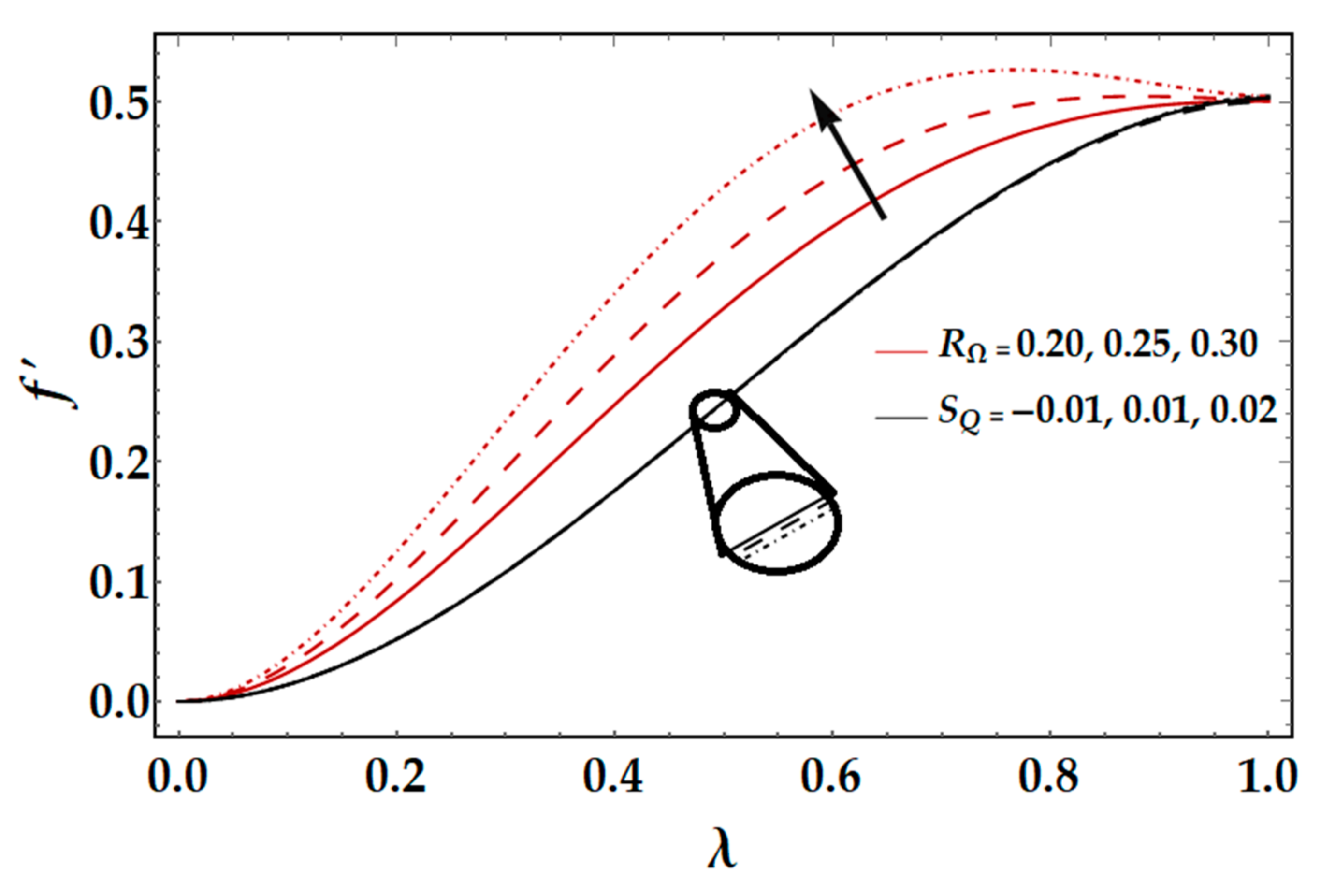
Figure 2 illustrates the influence of the velocity profile in the axial direction $f^{\prime }$ because of the squeezed Reynolds number $S_Q$, rotational Reynolds number $R_{\mathsf{\Omega }}$, and the material parameter of Reiner-Rivlin fluid $K$. From Figure 2 one can perceive that increasing the squeezed Reynolds number $S_Q$ axial velocity decreases, but increasing rotational Reynolds number $R_{\mathsf{\Omega }}$, the axial velocity profile increases. The physical reason behind this is that when we increase the value of Squeezing Reynolds number $S_Q$, the distance between the plates increases, the fluid velocity decreases, and the fluid accelerates by rotation of the plate when we increase the values of rotational Reynolds number $R_{\mathsf{\Omega }}$. Figure 3 depicts that increasing the values of the material parameter of the Reiner-Rivlin fluid increases the velocity distribution against axial direction $f^{\prime }$.

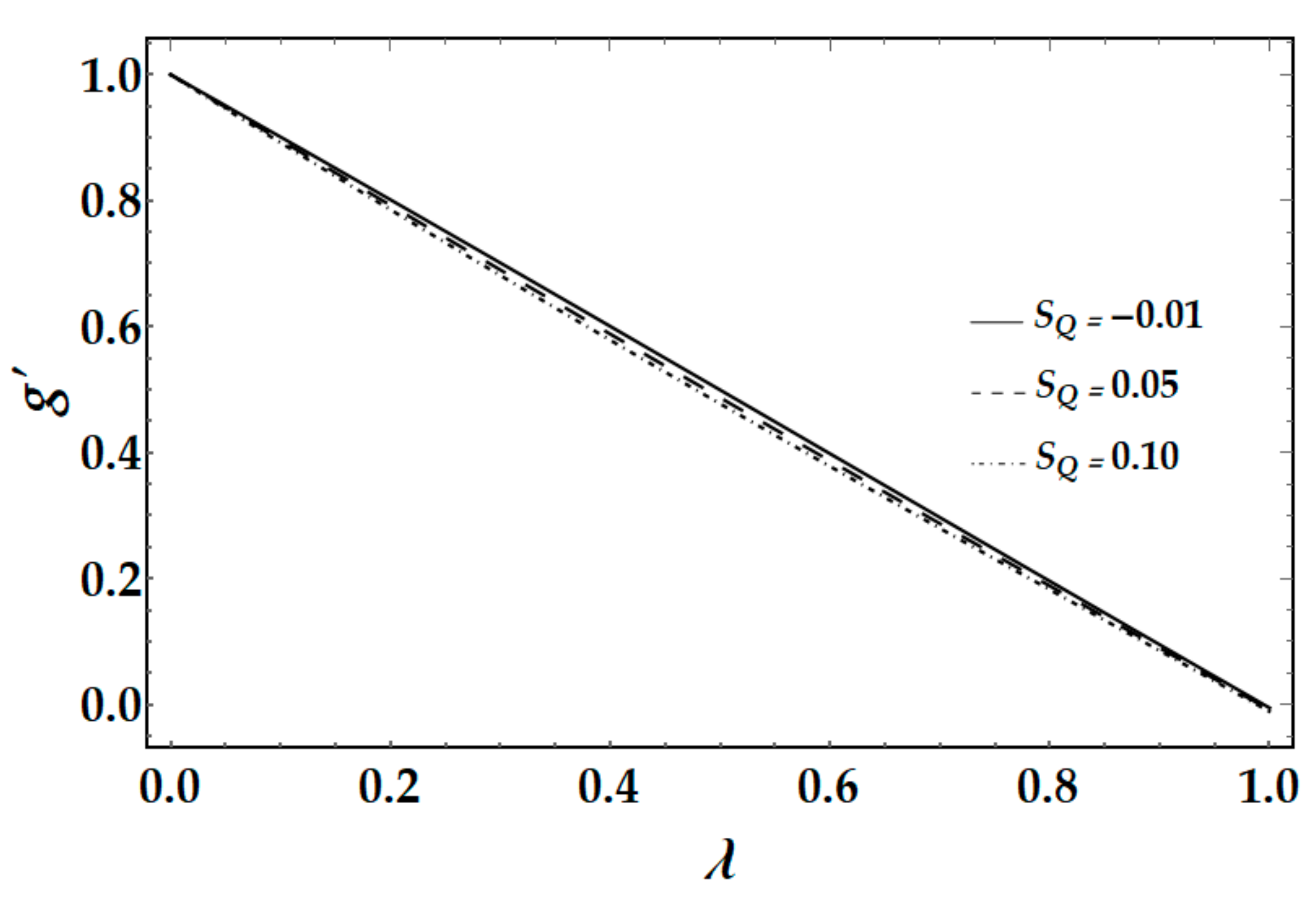
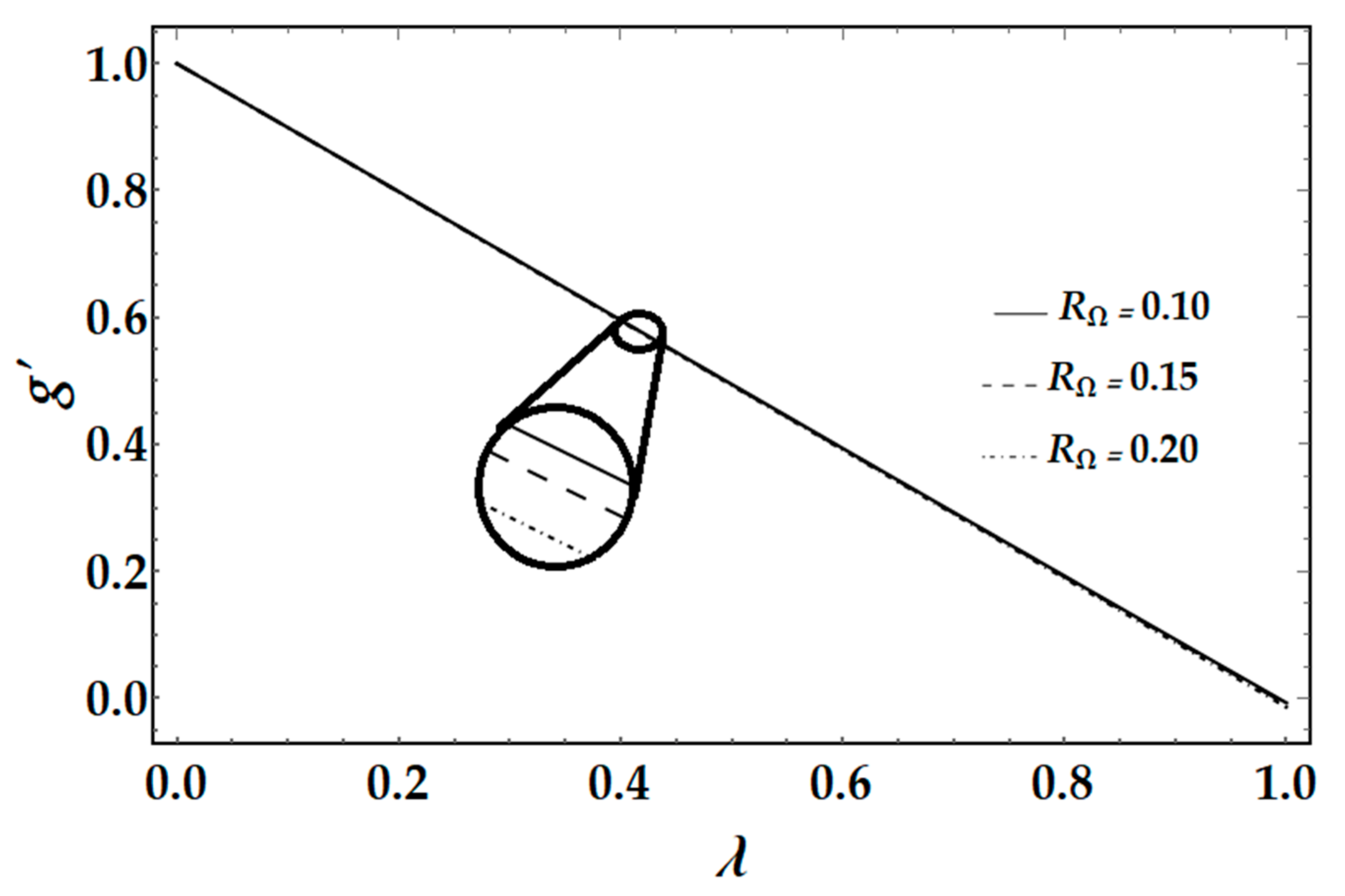
Figure 4 depicts the influence of squeezing Reynolds number $S_Q$ and Rotational Reynolds Number $R_{\mathsf{\Omega }}$ against tangential velocity distribution $g^{\prime }$. From Figure 4, it can be ascertained that by enhancing the values of the squeezed Reynolds number $S_Q$, the tangential velocity distribution decreases. Similar phenomena are observed in Figure 5, i.e., by increasing the values of the rotational Reynolds number, the tangential velocity profile declines.

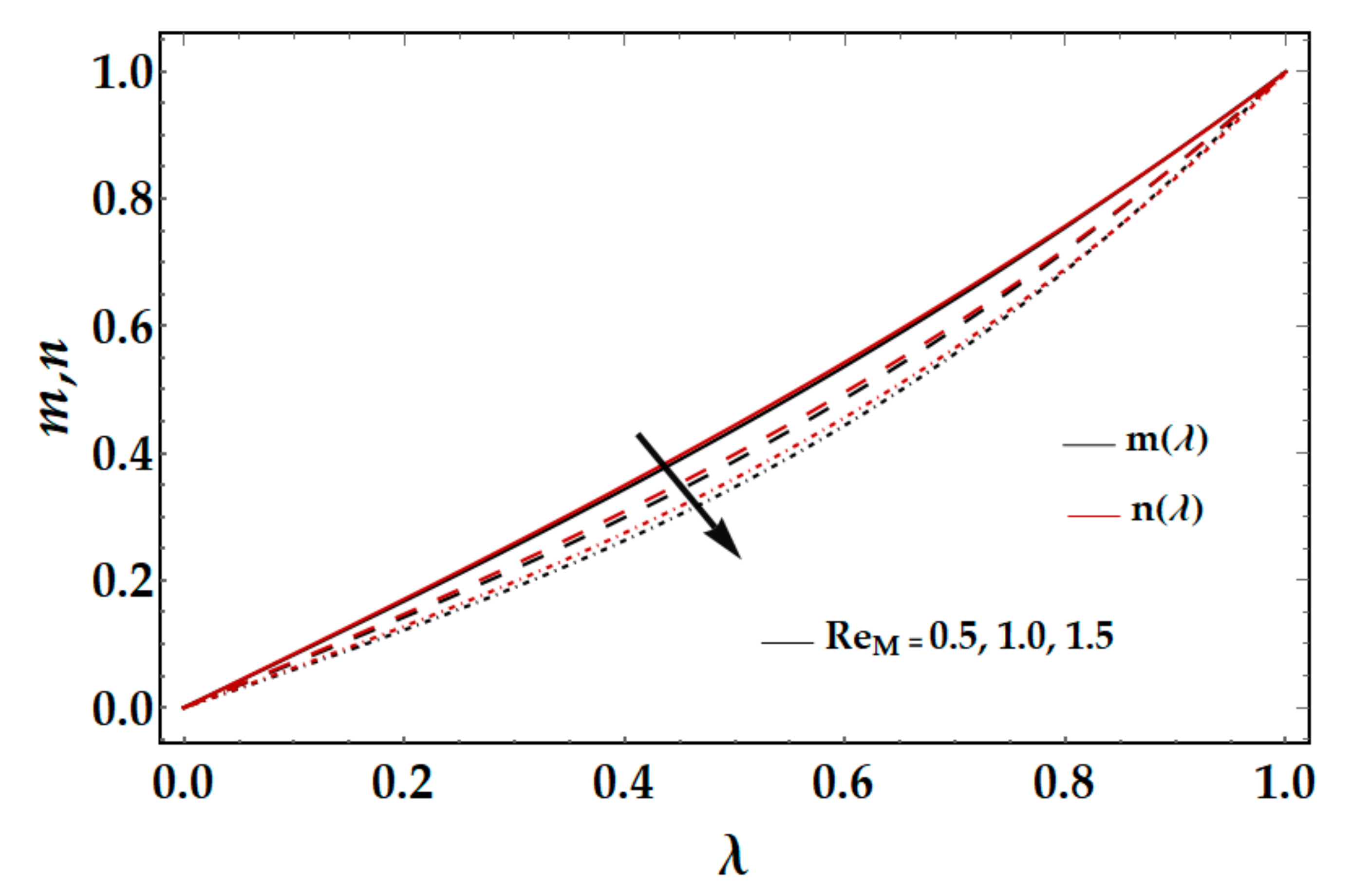
From Figure 6, it can be seen that by increasing the values of magnetic Reynolds number ${\mathrm{Re}}_M$, the tangential and axial magnetic field decreases, as the magnetic Reynolds number is the ratio of fluid flux to the mass diffusivity. So, by increasing the magnetic Reynolds number, a decrease in mass diffusivity and increase in fluid flux is seen. This decline in mass diffusivity disrupts the diffusion of the magnetic field and resulting, a decline in axial and tangential induced magnetic fields is observed.

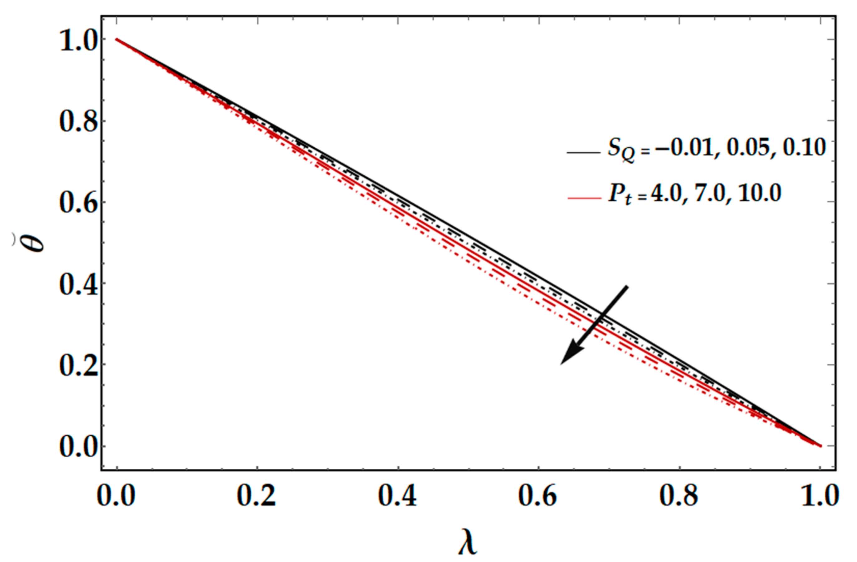
Figure 7 elucidates the consequences of the Brownian motion parameter and thermophoresis parameter $T_b,T_t$ on the temperature field $\stackrel{⌣}{\theta }$. The graph shows that intensifying the values of thermophoresis, Brownian motion parameter $T_t,T_b$ increases the temperature profile. The physical reason is that the fluid temperature increases due to strengthening the kinetic energy of nanoparticles. The effects of squeezing Reynolds number $S_Q$ and Prandtl number $P_t$ on temperature profile $\stackrel{⌣}{\theta }$ is displayed in Figure 8. One can notice that by enhancing the Prandtl number $P_t$ and the squeezing Reynolds number $S_Q$, the temperature profile $\stackrel{⌣}{\theta }$ diminishes. When the thermal conductivity reduces by intensifying the values of the Prandtl number $P_t$ then the temperature profile $\stackrel{⌣}{\theta }$ declines. 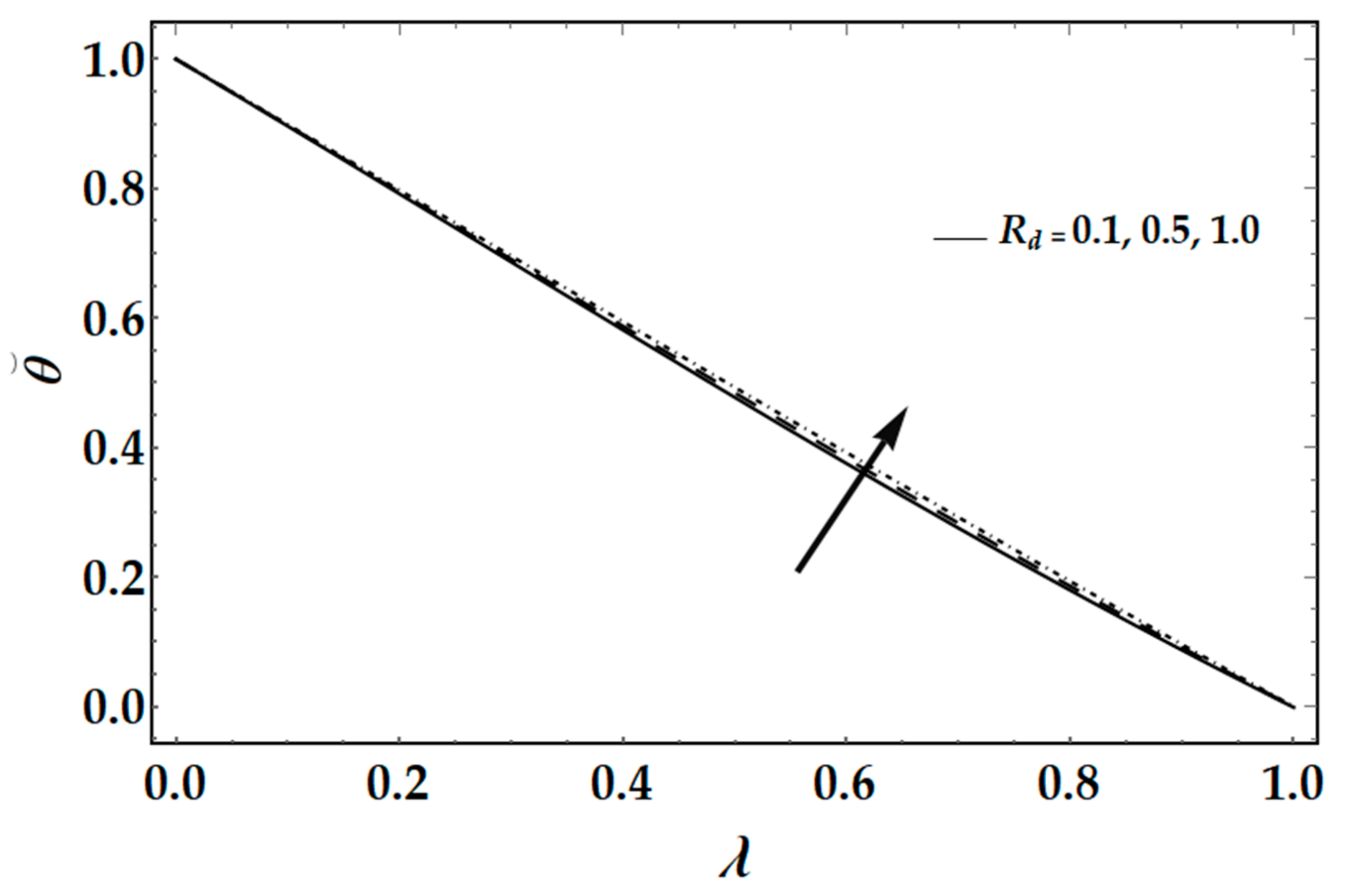The effects of radiation parameter $R_d$ on temperature profile $\stackrel{⌣}{\theta }$ are shown in Figure 9. It is observed that by enhancing the radiation parameter $R_d$ the temperature profile $\stackrel{⌣}{\theta }$ increases. The physical reason behind this is that an increase in radiation releases the heat energy from flow; hence there is an increase in temperature.

Figure 10 shows the consequences of thermophoresis parameter $T_t$ and Brownian motion $T_b$ on nanoparticle concentration $\varphi$. It is perceived that nanoparticle concentration declines by increasing the values of Brownian motion $T_b$, and concentration of nanoparticle intensifies by increasing values of thermophoresis parameter $T_t$. In fact, gradual growth in $T_b$ increases the random motion and collision among nanoparticles of the fluid, which produces more heat and eventually it results in a decrease in the concentration field. Due to increasing values of $T_t$, more nanoparticles are pulled towards the cold surface from the hot one, which ultimately results in increasing the concentration distributions. 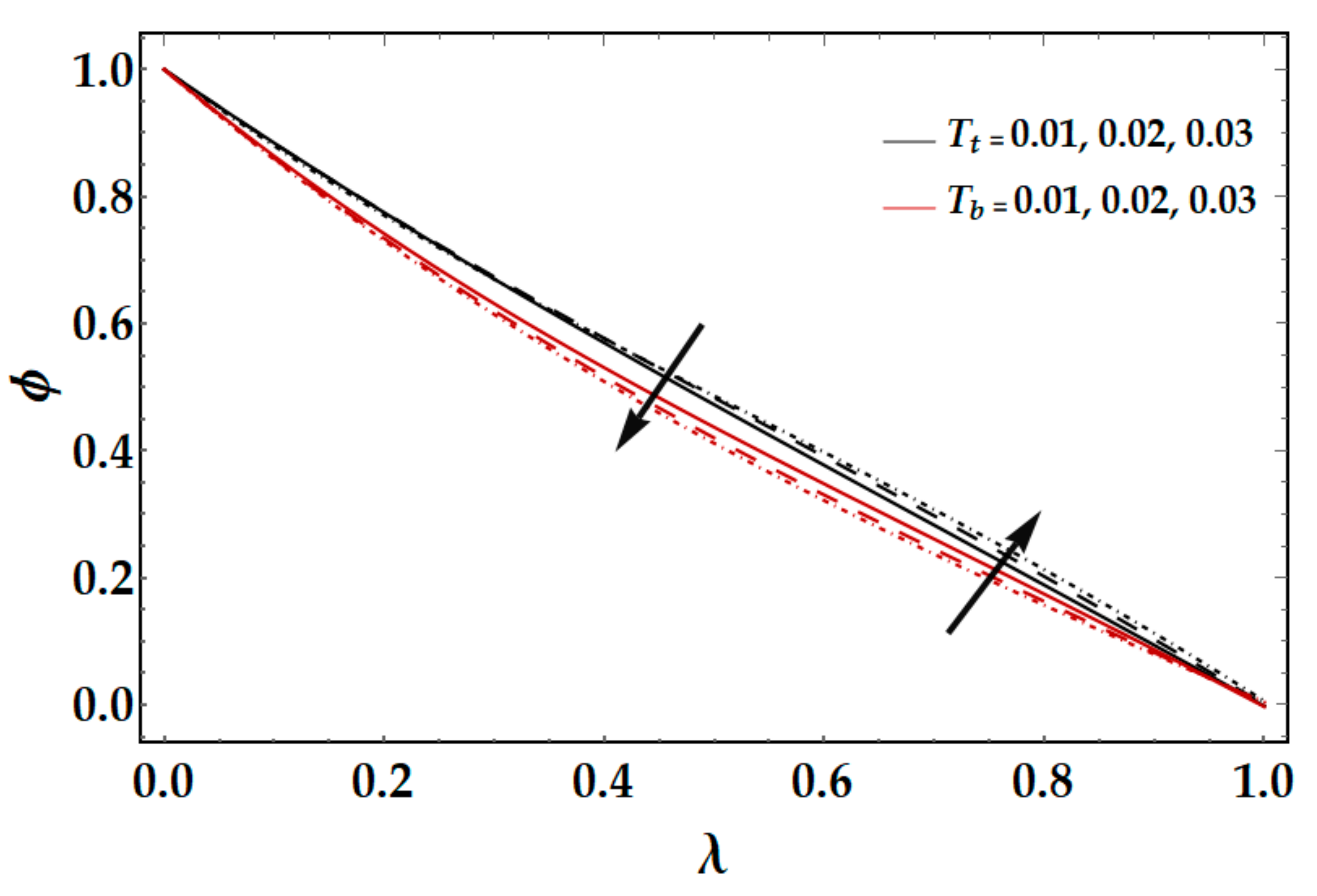Figure 11 shows the consequences of Schmidt number $S_M$ and squeezed Reynolds number $S_Q$ on nanoparticle concentration. By enlarging the values of squeezed Reynolds number $S_Q$, nanoparticle concentration $\varphi$ increases, on the other hand, converse phenomena are noticed by enhancing the values of Schmidt number $S_M$. 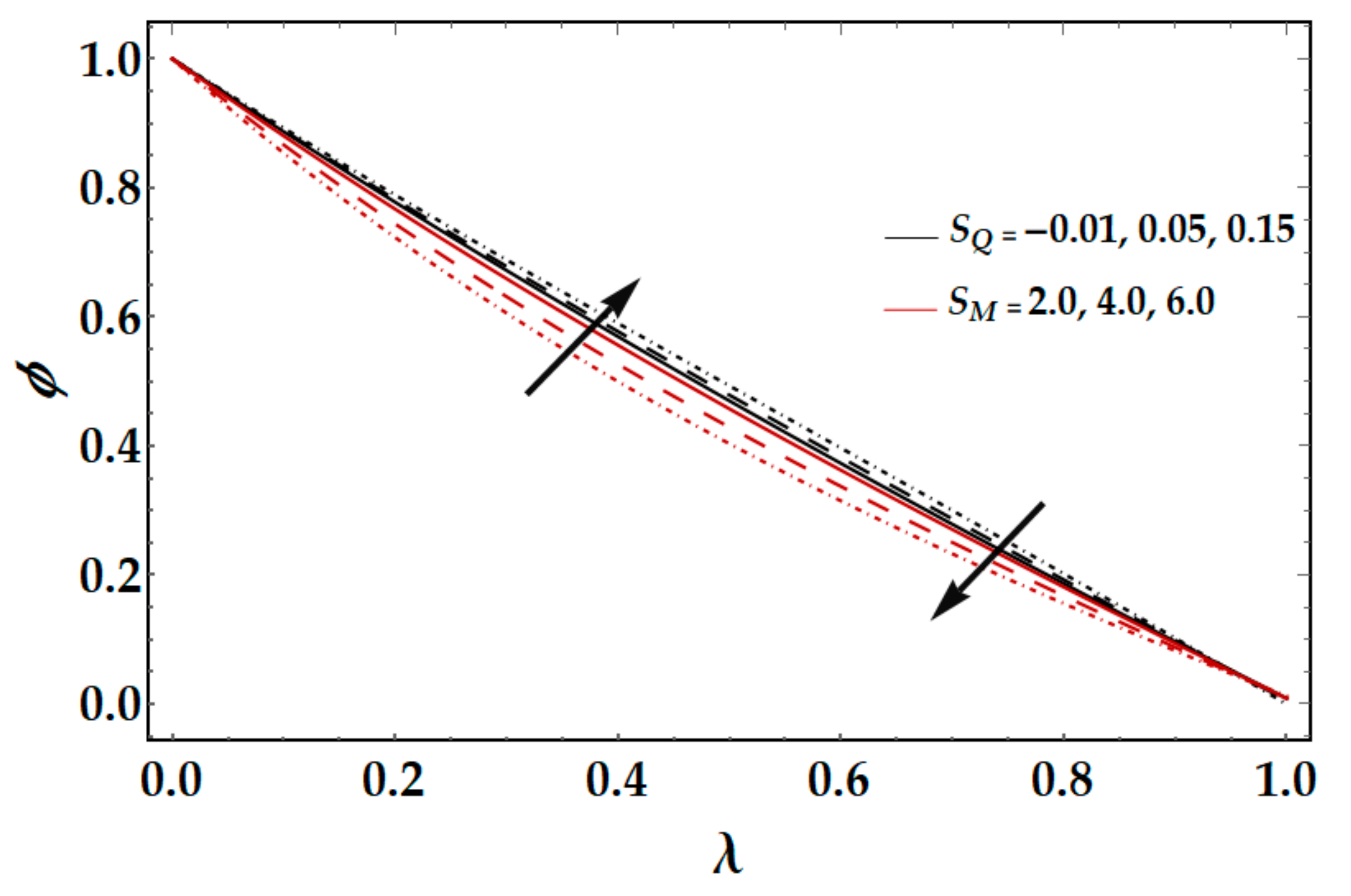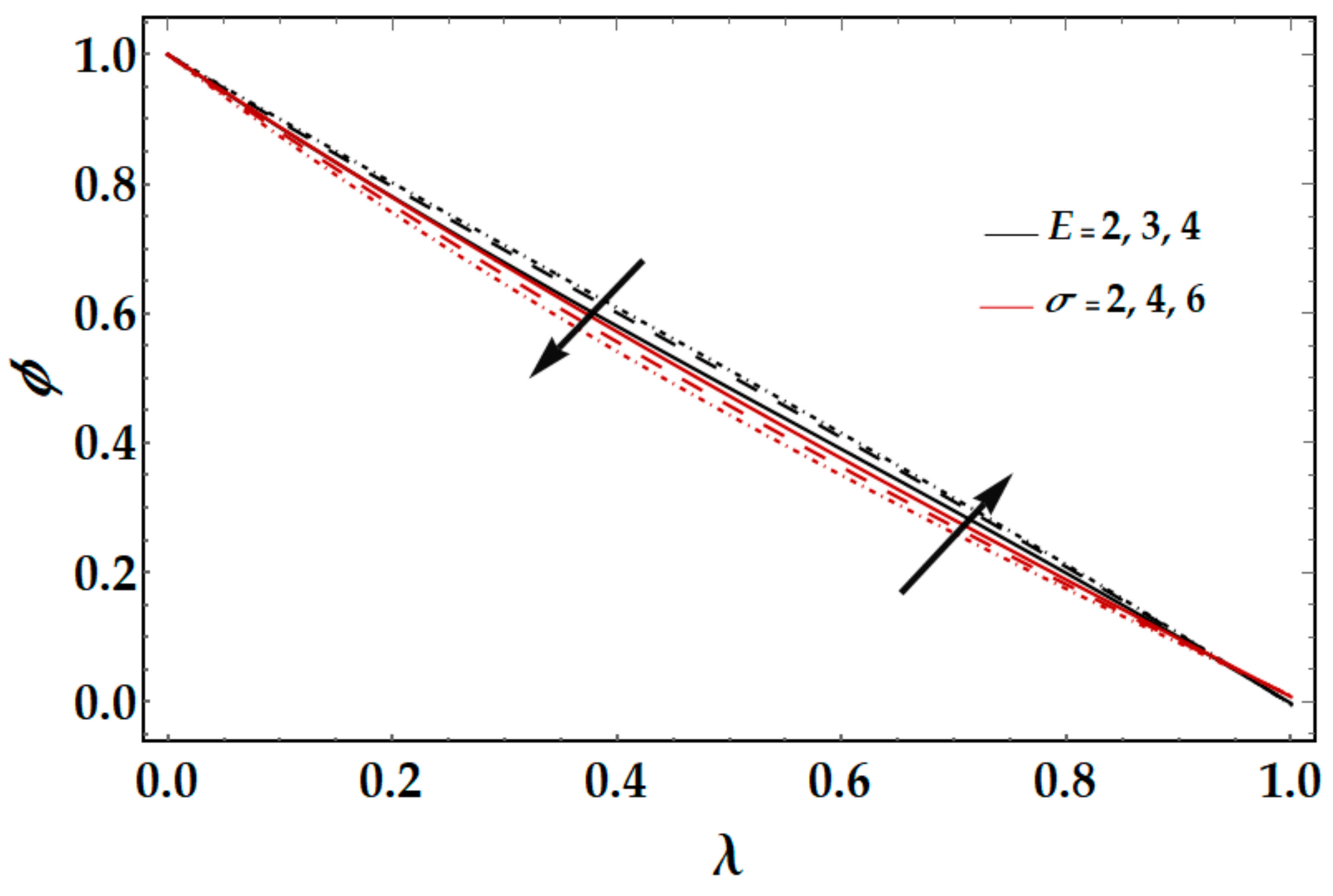Figure 12 deliberates the influence of reaction rate $\sigma$ and activation energy $E$ on the nanoparticle concentration $\varphi$. It may be observed that nanoparticle concentration displays a substantial rise by increasing values of $E$. Since high energy activation and low temperatures impart to a constant reaction rate, the resulting chemical reaction is therefore slowed down. Consequently, the concentration of the solute rises. On the other side, by increasing values of $\sigma$, the nanoparticle concentration decreases.

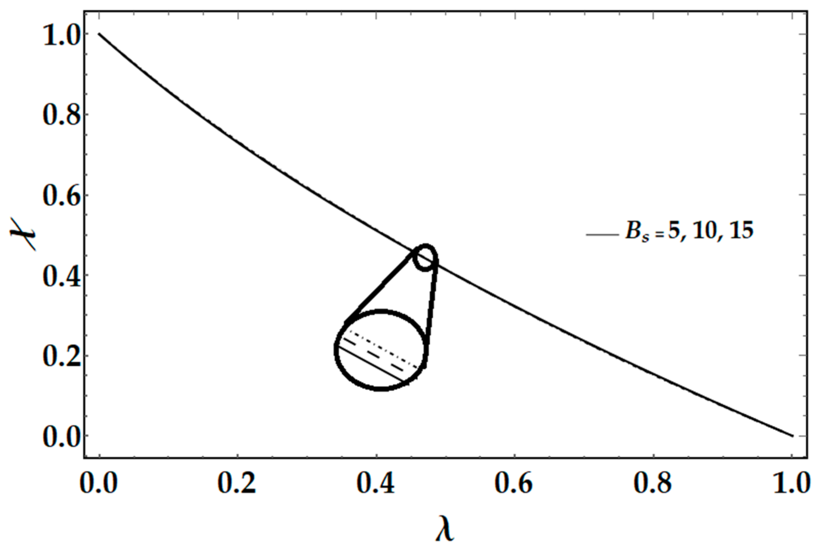
Figure 13 portrays the consequences of Peclet number $P_l$ and squeezed Reynolds number $S_Q$ on motile microorganism density function $\chi$. One can experience that enhancing values of squeezed Reynolds number $S_Q$ tends to boost the microorganism density function, while increasing the values of Peclet number $P_l$, the motile microorganism density function diminishes. The reason behind this is that the diffusivity of the microorganism reduces, then the speed of the microorganism also decreases. This is the physical fact and resulting in the microorganism density function decreasing while increasing the value of Peclet number $P_l$. Figure 14 is plotted to see the physical performance of the Bioconvection Schmidt number $B_s$. It is apparent that by enhancing values of bioconvection Schmidt number $B_s$ the motile microorganism density function rises, but the consequences are negligible.

6. Conclusions

In this study, we determined incompressible three-dimensional, unsteady, axisymmetric squeezed film flow of Reiner-Rivlin nanofluid between parallel circular plates. The impact of an induced magnetic field, the suspension of motile gyrotactic microorganisms, activation energy, and thermal radiation are also contemplated. DTM-Padé is applied to present the solutions of the ordinary differential equations after employing the similarity transformations. Padé approximant is applied because it provides a good rate of convergence and gives reliable results. Comparison is made for the values of toque on the lower and upper plates. The main findings are accomplished below:

• The opposite behavior is experienced for the rotational Reynolds number on tangential and axial velocity distribution.
• Enhancing the value of squeezing Reynolds number, the tangential and axial velocity distribution decreases.
• By enlarging the value of the magnetic Reynolds number, the magnetic field (induced) in tangential and axial directions decreases.
• The Reiner-Rivlin opposes the fluid motion; however, the impact is negligible.
• By increasing the Brownian motion and thermophoresis parameter, the temperature distribution rises.
• Temperature distribution decays due to the effects of the Prandtl number-like phenomenon is observed for enlarging the values of squeezed Reynolds number.
• The thermal radiation parameter enhances the temperature distribution.
• Nanoparticle concentration and motile density increase by enhancing the in value of squeezing Reynolds number.
• Nanoparticle concentration shows opposed phenomena for Brownian motion parameter compared with thermophoresis parameter.
• Increasing values of activation energy tends to intensify the nanoparticle concentration profile.
• The microorganism profile declines by increasing the values of Peclet number, but the microorganism profile rises by enlarging the bioconvection number.

Future Work: The present study shows perfect accuracy of the proposed methodology; however, attention has been given to non-Newtonian fluid with induced magnetic. Future studies may generalize the present study to consider applied magnetics effects, porosity effects, slip effects, entropy generation, and other non-Newtonian fluid models, etc., which are beneficial to bioreactor configurations and lubrication regimes and will be presented soon.