Abstract
The current article presents the entropy formation and heat transfer of the steady Prandtl-Eyring nanofluids (P-ENF). Heat transfer and flow of P-ENF are analyzed when nanofluid is passed to the hot and slippery surface. The study also investigates the effects of radiative heat flux, variable thermal conductivity, the material’s porosity, and the morphologies of nano-solid particles. Flow equations are defined utilizing partial differential equations (PDEs). Necessary transformations are employed to convert the formulae into ordinary differential equations. The implicit finite difference method (I-FDM) is used to find approximate solutions to ordinary differential equations. Two types of nano-solid particles, aluminium oxide (Al2O3) and copper (Cu), are examined using engine oil (EO) as working fluid. Graphical plots are used to depict the crucial outcomes regarding drag force, entropy measurement, temperature, Nusselt number, and flow. According to the study, there is a solid and aggressive increase in the heat transfer rate of P-ENF Cu-EO than Al2O3-EO. An increment in the size of nanoparticles resulted in enhancing the entropy of the model. The Prandtl-Eyring parameter and modified radiative flow show the same impact on the radiative field.
1. Introduction
Nanofluids, including nanomaterial dispersed in a pure fluid, are becoming applicable fluids in various systems due to their proved superior specification [1]. Augmented thermal conductivity is a remarkable property induced from nanofluid as compared with conventional fluids [2]. On the other hand, the viscosity of nanofluids is significantly varied depending on the type of nanoparticles, base fluid, and their interaction [3]. Some authors have observed Newtonian behaviour of nanofluids, while a non-Newtonian one has been widely revealed [4]. The non-Newtonian behaviours have practical implementations in wire and blade coating, molten plastic, dyeing of textile, some petroleum fluids, biological fluids movement, and food and slurries processing. In this regard, various kinds of rheological behaviours can be expected, defined by models such as power law, micropolar, Reiner–Philippoff, viscoelastic, Casson, Carreau, Giesekus, Prandtl, Prandtl–Eyring, and Powell–Eyring [5]. These models introduce special impendence on the momentum conservation equations to be compatible with the targeted behaviour. Indeed, in mathematical language, the relationship between shear stress and deformation rate is described by each model. Prandtl and Prandtl–Eyring are a function of sine inverse and sine hyperbolic, respectively [6,7]. The power law model characterizes the relation as nonlinear [8]. Sajid et al. [9] studied a micropolar Prandtl fluid for a porous stretching sheet situation. They assumed that the heat source is related to temperature and a chemical reaction occurs into the medium. Maleki et al. [10] performed numerical research on power law nanofluid, which flows on a porous plate. They found that using Newtonian nanofluid has no improvement effect on heat transfer.
In contrast, the non-Newtonian one had an essential role in boosting heat transfer. Shankar and Naduvinamani [11] worked on the transport phenomena of a Prandtl–Eyring fluid through a sensor surface under magnetic force conditions. The observation showed that magnetic parameter augmentation causes a velocity field increment and temperature profile reduction. At the same time, heat transfer diminished by the Prandtl number rose. Temperature and concentration variations on Prandtl–Eyring fluid heat transfer were investigated by Al-Kaabi and Al-Khafajy [12] in a porous medium. Finally, Hayat et al. [13] evaluated the efficacy of Prandtl–Eyring nanofluid on gyrotactic microorganisms in a stretching sheet. The results indicated that higher melting parameters hike the velocity and pull down the temperature.
Stretching surface is a well-known and habitual process in industrial situations, i.e., extrusion, fiberglass, cooling of the metallic plate, glass blowing, hot rolling, etc. Boundary layer flow and heat transfer is the theory that helps better understand the scientific phenomena underlying it [14]. Nonlinear equations are expected from practical problems which are experienced in engineering applications. The Keller box method is an implicit finite difference method used to solve these types of equations [15]. Munjam et al. [16] proposed a new technique to solve the fluid flow of a Prandtl–Eyring fluid on a stretched sheet and compared their results with the Keller box method. The analytical outcomes indicated that as the fluid parameter rises, velocity enhances. In addition, they found that the Prandtl–Eyring fluid induces a grosser velocity value as compared to the viscous one.
Jamshed et al. [17] explored the entropy generation of Casson nanofluid by considering the Tiwari and Das model and the Keller box method to solve ODEs. Two methanol-based nanofluids were used by introducing Cu and TiO2 nanoparticles; Cu nanofluids showed a better performance. In [18], they also used the same models and techniques for the same nanoparticles for engine oil base fluid. They concluded that entropy generation would enhance by Reynolds number and Brinkman numbers. Moreover, increasing nanofluid concentration led to shear rate enhancement. Abdelmalek et al. [19] discussed a Prandtl–Eyring nanofluid which influences Brownian motion and thermophoretic force through a stretched surface. It was proved that magnetic force is undesirable for the momentum. In contrast, Brownian motion and thermophoretic force raised the thermal energy.
In the viewpoint of heat transfer, thermal conductivity is a determinant parameter that is generally assumed to be unchanged. However, extensive studies emphasized that the efficacy of temperature changing the thermal conductivity would vary. Particularly, nanofluids have an intimate relation with temperature, which can considerably affect the heat transfer due to the higher aspect ratio that nanoparticles provide within the base fluid. It is proved that at higher temperatures, the thermal conductivity is typically more elevated. Thus, in a range of temperatures, the thermal conductivity is variable. Maleki et al. [20] studied the efficacy of different kinds of nanofluids on the heat transfer of a porous system. They claimed that the results are opposite with other researchers, i.e., adding more nanoparticles dwindled the heat transfer because it can alter radiation, viscous dissipation, and heat generation. In [21], they also surveyed the non-Newtonian nanofluids by considering the mixture of CMC and water as a base fluid. It was revealed that using non-Newtonian nanofluid in injection mode has a higher heat transfer efficiency as compared to the Newtonian one. Jamshed et al. [22] investigated Casson nanofluid in a stretching sheet system that included variable thermal conductivity. Keller box was the technique that solved ODEs. In this method, differential equations are solved numerically to reduce them into the 1st order differential equations. They used TiO2 and Cu as nanoparticles in water. Cu/water nanofluid had better heat conduction performance. Carreau–Yasuda nanofluid was researched by Waqas et al. [5] by considering gyrotactic motile microorganisms. Velocity, thermal, and temperature fields were amended by decreasing the bioconvection Rayleigh number, increasing the thermal Biot number, and decreasing the Prandtl number. In addition, the concentration field improved by reducing Brownian motion. Xiong et al. [23] explained that variable thermal conductivity has a determinant role in field quantities. They scrutinized a fibre-reinforced generalized thermoelasticity system by considering temperature-dependent thermal conductivity. Ibrahim and Negera [24] inspected an MHD Williamson nanofluid effect within a stretching cylinder by considering chemical reaction conditions. They asserted that the higher the parameter of variable thermal conductivity, the higher the Sherwood number and skin friction, while the lower the Nusselt number. Dada and Onwubuoya [25] analysed an MHD Williamson fluid over a stretchable surface of variable thickness and thermal conductivity. The conclusion indicated that rising changeable thermal conductivity improves temperature. Hasona et al. [26] described the variable thermal conductivity of a non-Newtonian nanofluid in a special geometry channel. They reported that rising thermal and electrical conductivities enhance the temperature of working fluid, which in turn augments heat transfer performance within the system. Fatunmbi and Okoya [27] presented an investigation on hydromagnetic Casson nanofluid at the attendance of thermophoresis, ohmic heating, and a nonuniform heat source with variable thermal conductivity for a stretching sheet system. They demonstrated that driving up the Casson fluid parameter dwindled the fluid flow velocity, albeit, it augmented the viscous drag.
After a glance into the erstwhile studies, since most industrial fluids include non-Newtonian fluids in a situation like stretching surface, the significant concerns of the current project are to discuss the Prandtl–Eyring nanofluid flow over a stretching sheet under three conditions of variable thermal conductivity, thermal radiative flow, and porous material. In addition, their effects on the entropy formation were elaborated by considering the Tiwari and Das model. In this way, Al2O3/EO and Cu/EO nanofluids were analysed at volume concentrations of 3% to 20%. Furthermore, this study implemented the implicit finite difference method to solve the boundary layer equations nicely. Therefore, it can be said that the valuable outcomes of this research can be a guideline for practical applications because it was conducted to select parameters close to actual industrial conditions.
2. Flow Model Formulations
A nonregular stretching velocity was used in the flow analysis to characterize horizontal surface movement (for instance, Reference [28]):
where m is a pilot spreading ratio. The temperature at the surface is For the sake of adaptability, it was fabricated as a perpetual at x = 0. m*, and provided the temperature variation rate, thermal disparity rate, and ambient temperature congruently.
2.1. Prandtl–Eyring Fluid Stress Tensor
Prandtl–Eyring fluid stress tensor can be expressed as follows (Qureshi [29]),
Here, signify extra stress tensor and indicates the flow velocity vector. and are fluid parameters. The complete derivation of this specific stress tensor and velocity field can found in Becker [30].
2.2. Model Assumptions and Restraints
The mathematical model was taken into account in the following presumptions and requirements:
- ✓
- 2D laminar flow
- ✓
- Boundary layer estimation
- ✓
- Tiwari and Das nanofluid model
- ✓
- Non-Newtonian Prandtl–Eyring nanofluid
- ✓
- Copper (Cu) and aluminium oxide (Al2O3) nanoparticles
- ✓
- Base fluid is engine oil (EO)
- ✓
- Variable thermal conductivity
- ✓
- Thermal radiation
- ✓
- Permeable stretching surface
- ✓
- Convective and slippery velocity conditions.
2.3. Geometry for Single-Phase Flow Model
Following is the geometric flow model: the flow goes over the sheet. Thermal leap was used to transfer heat from the fluid’s surface to the fluid’s inside as the velocity at the surface underwent the flow slip event. Alumina oxide nanoparticles and copper nanoparticles were mixed into the engine oil (see Figure 1).
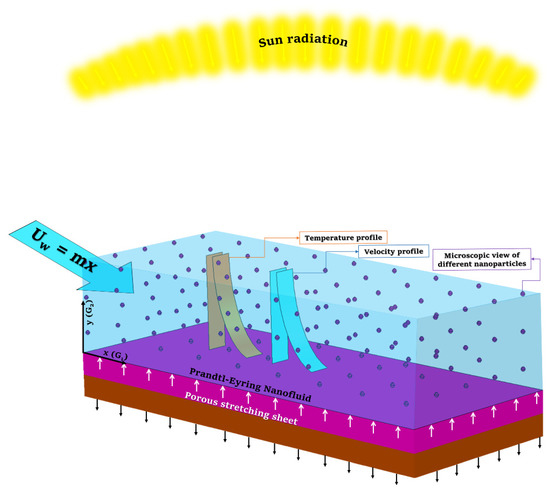
Figure 1.
Diagram of the single-phase flow model.
2.4. Classical Equations
The flow formulae of viscous and steady Prandtl–Eyring nanofluid (P-ENF) in combination with variant thermal conductivity, radiation, and porous material are [31,32,33].
the appropriate connection conditions were as follows (Aziz et al. [34]):
is the temperature of the nanofluid.
Other crucial parameters involved fluid parameters , slip length surface permeability , heat transfer coefficient , and porosity along with heat conductivity of firm . It considered physical elements such as the thermal loss from a conventionally heated surface due to conduction and velocity at the surface as a function of the shear stress applied to it (slip condition). Because of the thickness of non-Newtonian P-ENF, just a short distance was covered by the radiative flow. Therefore, radiation heat flux estimation obtained through Rosseland [35] was applied in Equation (5).
herein, represents the Stefan–Boltzmann constant. Table 1 summarizes the equations of P-ENF material variables [36,37]:

Table 1.
Formulae used for studied nanofluids [36,37].
Table 2.
Materials thermophysical properties [38,39].
3. Dimensionless Formulations Model
Similarity transformations that convert the governing PDEs into ODEs, and the BVP formulae (3)–(7) are modified. Familiarizing stream function in the equation [28]
The specified similarity quantities are ([28])
into Equations (3)–(7). We get
with
where is in formulae (11)–(12) signify the subsequent thermophysical structures for P-ENF [29].
Equation (2) is clearly shown to be valid. Table 3 shows the needed derivatives.
Table 3.
Entrenched Control Constraints.
Other parameters like skin friction , Nusselt number and entropy generation ( can be expressed as [31,32]:
4. Implicit Finite Difference Method
The implicit finite difference method (I-FDM) [40] was utilized to obtain the numerical solution for the equation set of models. I-FDM has an advantage as it has fast convergence. It is 2nd order convergent and inherently stable. I-FDM satisfies the Von Neumann stability test, which has the criterion of a real numerical solution for PDEs with the help of the stability and consistency of a numerical solution. I-FDM is employed to obtain the solution of Equations (11) and (12) using boundary conditions (13). This is a suitable method to obtain the approximated solution of boundary layer problems. I-FDM is widely applicable in the flow problems of the laminar boundary layer, and the obtained results are more effective than others.
To apply the implicit finite difference method [41], Equations (11) and (12) were written in the form of 1st order differential equations utilizing newly employed variables. Reduced equations are as follows [32]:
With the presence of newly employed variables, boundary conditions eventually changed to [31]
The different formulae were calculated using central differencing, and average functions were replaced. Thus, the 1st ODEs (16) and (20) order decreases to the next series of nonlinear algebraic formulae.
To linearize the resulting equations, Newton’s technique was used. As an example, consider iteration (i + 1)th
under the substitutition of the linear tridiagonal equational system into Equations (22)–(26), disregarding the elevated components.
where
The boundary conditions become
The following are the formulae (33)–(37) that produce the bulk tridiagonal array,
where
This matrix, , resembles the generalized size of , whereas the and indicate the column vectors order of . Afterward, a unique LU factorization approach was employed to get the solution for
5. Code Validity
The technique’s authenticity was assessed by comparing the thermal conveyance rate fallouts between the recent scheme and the previous results [42,43,44,45]. Table 4 summarises the consistency relationship found in all of the studies. Therefore, the findings of the present study are agreeable with previously published results and verified.
Table 4.
Comparison of with , whenever , , , , and .
6. Results and Discussion
The section discusses the numerical outcomes obtained on the model in consideration. The parameters involved in the results are , , , S, , and . Figure 2, Figure 3, Figure 4, Figure 5, Figure 6, Figure 7, Figure 8, Figure 9, Figure 10, Figure 11, Figure 12, Figure 13, Figure 14, Figure 15, Figure 16, Figure 17, Figure 18, Figure 19, Figure 20 and Figure 21 display the physical behavior of the mentioned parameters regarding energy, entropy formation, and velocity on the nondimensional entities of the model. Results for non-Newtonian Al2O3-EO and Cu-EO P-ENFs were obtained. Temperature differences and coefficient of skin fraction are detailed in Table 5. The values used for the parameters are , , , S , , and The power of Al2O3-EO and Cu-EO were decided with the fractional size of nanoparticles used in the working fluid. Flow stability of nanoparticles decreased when nanoparticles had a higher amount of fractional range. Al2O3-EO was favored more by fractional improvement than Cu-EO nanofluid. Figure 2 shows a lower flow of Cu-EO nanofluid than Al2O3-EO. As Al2O3 has a high heat transfer property, its primary purpose is to combine with EO. When the fractional volume of both fluids flows increases, thermal distribution transported to the domain from the surface is high, as shown in Figure 3. The increasing fractional volume also resulted in enhancing the fluctuations of the system entropy. Figure 4 shows the leading fluctuations of Cu-EO nanofluid, which settled down midway and increased further towards Al2O3-EO nanofluid. The thermal radiation parameter models the radiation procedure used in enhancing the entropy rate and heat regarding induced temperature, as shown in Figure 5 and Figure 6. Radiations had a negligible effect on the entropy variations caused by the prominent influence of flow conditions. Cu-EO had more control than the Al2O3-EO nanofluid. Regarding heat capability of Al2O3 and Cu-EO nanofluids, there was a dominant effect on entropy and thermal aspects of individual variations in i.e., thermal conductivity. Figure 7 and Figure 8 represent these effects. When the variation parameter tries to increase the ranges of entropy and heat, the nominal impact of is proved by close variations of entropy and thin layers of heat. In both behaviors of parameters, Al2O3-EO underestimated the Cu-EO nanofluid. Figure 9 and Figure 10 clearly show the increment in convective heat on thermal as well as entropy states from lower surfaces in the domain. Parametric values of Biot number represent the ordinary heating procedure . An increase in resulted in enhancing the thermal state in the flow domain, but this only had a negligible impact on the entropy generation. The entropy profile is smaller than the thermal boundary layer, which proves the above statement. According to the study, Al2O3-EO is better than Cu-EO nanofluid. Figure 11, Figure 12 and Figure 13 demonstrate the impact on the power, entropy, and velocity distributions of Prandtl–Eyring nanofluid . Figure 11 shows the speed () corresponding to . The velocity of both fluids increased with amplification in . However, the velocity of Al2O3-EO velocity was more incredible as compared to Cu-EO. Figure 12 shows the temperature curve concerning the Prandtl–Eyring parameter . An increment in resulted in reducing the temperatures of both fluids. However, the temperature profile of Cu-EO nanofluid is more critical than Al2O3-EO nanofluid. Figure 13 represents the entropy fluctuation of P-ENF caused by . An increase of resulted in lowering the entropy formation. The lower value of entropy of the Al2O3-EO fluid was used to represent Cu-EO nanofluid when both nanofluids were at the end of the graph. is strongly related to the profile of P-ENF. However, an increase of resulted in decreasing the entropy and temperature. Figure 14, Figure 15 and Figure 16 illustrate the efficacy of the Prandtl–Eyring parameter on the profiles of temperature, velocity, and entropy formation. The velocity change regarding was displayed in Figure 16. A decrease in the velocity profile was the result of an increment in Cu-EO while increasing Al2O3-EO and a high rate in . Figure 15 shows the fluctuations in the profile of temperature concerning . The temperature grows as is increased, and Cu-EO obtains a quick temperature. Figure 16 highlights the difference in entropy caused by the Prandtl–Eyring parameter . An increment in entropy is obtained with increasing . Results obtained from modifying the slip conditions on the nature of the flow, heat, and generation of entropy, respectively, are shown in Figure 17, Figure 18 and Figure 19. Viscous behavior was focused on the flow conditions in the combinations of the Prandtle-Eyring fluid. Variations in velocity, entropy formation, and thermal distributions have an essential role in slip conditions. The situation for fluidity becomes difficult when slip conditions of Prandtl–Eyring fluid flow are increased. Fluidity was reduced for Cu-EO than Al2O3-EO P-ENF. Such hierarchy mainly occurs in thermal distributions, i.e., Cu-EO has a higher thermal state than Al2O3-EO nanofluid, as depicted in Figure 18. Greater values of slip parameter resulted in decreasing the entropy generation. It was caused by slip flow, which acted opposite to entropy generation, as shown in Figure 19. Figure 20 shows the performed estimations for = 0.6, 1.6, and 2.6; meanwhile, parametric values of are 0.2, 0.4, and 0.6. An increment in the material parameter resulted in enhancing the coefficient of skin friction. Flow velocity was decreased due to an increase in skin friction as resistance in fluid increased. In Figure 21, calculations for = 0.1, 0.3, and 0.5 were employed while Prandtl number was kept fixed on 1.0, 6.2, and 7.38. The convective heat transfer rate rose whenever the radiation parameter is increased. The heat transfer rate was augmented when heat flux was increased.
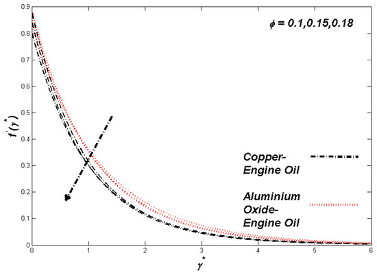
Figure 2.
Velocity variation with ϕ.
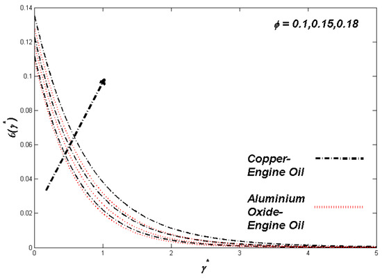
Figure 3.
Temperature variation with ϕ.
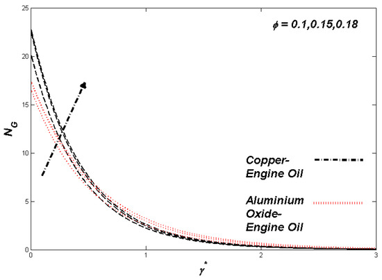
Figure 4.
Entropy variation with ϕ.
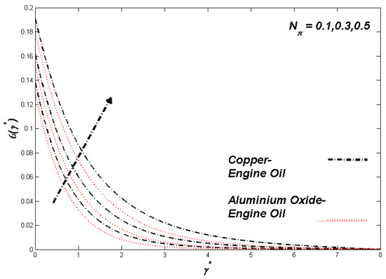
Figure 5.
Temperature variation with Nπ.
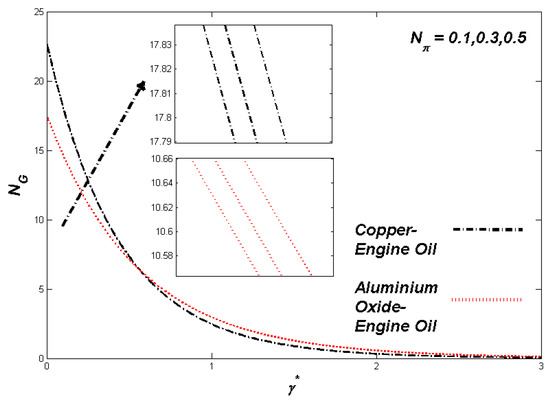
Figure 6.
Entropy variation with Nπ.
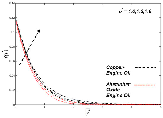
Figure 7.
Temperature variation with υ*.
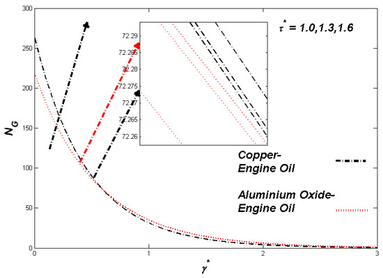
Figure 8.
Entropy variation with υ*.
Figure 9.
Temperature variation with Bπ.
Figure 10.
Entropy variation with Bπ.
Figure 11.
Velocity variation with τ*.
Figure 12.
Temperature variation with τ*.
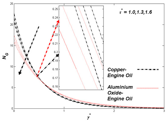
Figure 13.
Entropy variation with τ*.
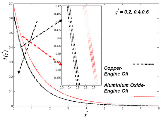
Figure 14.
Velocity variation with ς*.
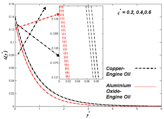
Figure 15.
Temperature variation with ς*.
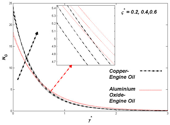
Figure 16.
Entropy variation with ς*.

Figure 17.
Velocity variation with Λπ.
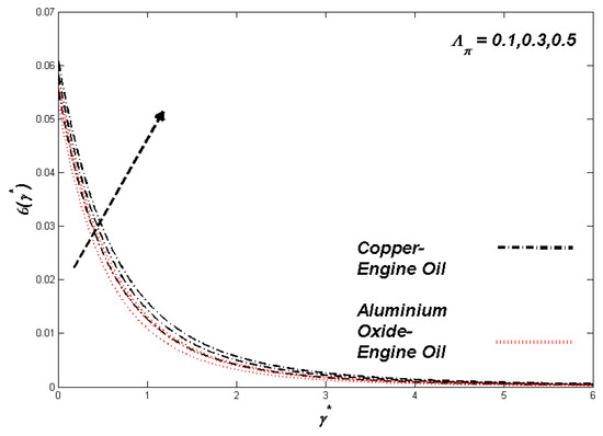
Figure 18.
Temperature variation with Λπ.
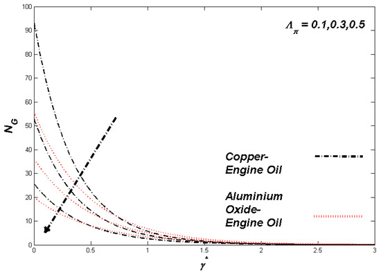
Figure 19.
Entropy variation with Λπ.
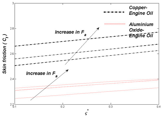
Figure 20.
Skin friction Cƒ against the parameter ς*.
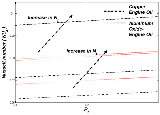
Figure 21.
Nusselt number Nux against the parameter Pr.
Table 5.
Values of and for .
7. Final Remarks
Investigations were made on HT properties and the entropy formation of P-ENF using a stretchable sheet. The single-phase method was employed to construct a computational model. Various physical parameters extract the results with the variations in energy, entropy, and velocity. The impacts of the thermal conductivity parameter , the thermal radiative parameter , Prandtl–Eyring parameters and the velocity slip parameter Biot number ,, and , as well as nanomolecular size and porous media parameter were examined in the study. Some of the main developments from the study were: The increment in the size of nanoparticles resulted in amplifying the heat transfer rate in engine oil. According to the analysis, copper nanofluid is a better heat conductor than aluminium oxide nanofluid. Increasing the porous media parameter , thermal radiative flow , size parameter , and Brinkman number the entropy was also enhanced. However, entropy was diminished with a rise in velocity slip parameter . An increment in the porous media parameter resulted in increasing the velocity. At the same time, it decreased with the nanoparticles’ size augmentation.
The results obtained from the present study can help future researchers improve the heat effect. Heating systems can be formed using various non-Newtonian nanofluids, including Casson, Carreau, second-grade, Maxwell, micropolar, etc. The efficacy of time-dependent porosity and viscosity along with magneto slip flow can be represented by expanding the study.
Author Contributions
Conceptualization, N.H.A.-H. and M.R.S.; methodology, N.H.A.-H.; software, K.H.A. and A.A.A.; validation, M.A.E.; formal analysis, K.A.A. and M.A.E.; investigation, resources, K.H.A.; visualization, A.A.A. and K.H.A.; data curation, K.A.A., writing—original draft preparation, A.M.A.; writing—review and editing, M.R.S. and K.A.A.; supervision, N.H.A.-H. and M.R.S.; project administration, A.A.A. and N.H.A.-H.; funding acquisition, M.R.S. and N.H.A.-H. All authors have read and agreed to the published version of the manuscript.
Funding
The authors extend their appreciation to the Deputyship for Research & Innovation, Ministry of Education in Saudi Arabia for funding this research work through the project number “IFPNC-006-135-2020” and King Abdulaziz University, DSR, Jeddah, Saudi Arabia.
Institutional Review Board Statement
Not applicable.
Informed Consent Statement
Not applicable.
Data Availability Statement
Not applicable.
Acknowledgments
The great help from King Abdulaziz University’s faculty members, including Radi A. Alsulami, Muhyaddin J. H. Rawa, Mashhour A. Alazwari, and Hatem F. Sindi are really appreciated.
Conflicts of Interest
The authors declare no conflict of interest.
References
- Zhang, X.; Tang, Y.; Zhang, F.; Lee, C.S. A novel aluminum–graphite dual-ion battery. Adv. Energy Mater. 2016, 6, 1502588. [Google Scholar] [CrossRef] [Green Version]
- Hosseini, S.M.; Safaei, M.R.; Goodarzi, M.; Alrashed, A.A.; Nguyen, T.K. New temperature, interfacial shell dependent dimensionless model for thermal conductivity of nanofluids. Int. J. Heat Mass Transf. 2017, 114, 207–210. [Google Scholar] [CrossRef]
- Ahmadi, M.H.; Mohseni-Gharyehsafa, B.; Ghazvini, M.; Goodarzi, M.; Jilte, R.D.; Kumar, R. Comparing various machine learning approaches in modeling the dynamic viscosity of CuO/water nanofluid. J. Therm. Anal. Calorim. 2020, 139, 2585–2599. [Google Scholar] [CrossRef]
- Bahiraei, M.; Salmi, H.K.; Safaei, M.R. Effect of employing a new biological nanofluid containing functionalized graphene nanoplatelets on thermal and hydraulic characteristics of a spiral heat exchanger. Energy Convers. Manag. 2019, 180, 72–82. [Google Scholar] [CrossRef]
- Waqas, H.; Farooq, U.; Khan, S.A.; Alshehri, H.M.; Goodarzi, M. Numerical analysis of dual variable of conductivity in bioconvection flow of Carreau–Yasuda nanofluid containing gyrotactic motile microorganisms over a porous medium. J. Therm. Anal. Calorim. 2021, 145, 2033–2044. [Google Scholar] [CrossRef]
- Wang, X.; Li, C.; Zhang, Y.; Said, Z.; Debnath, S.; Sharma, S.; Yang, M.; Gao, T. Influence of texture shape and arrangement on nanofluid minimum quantity lubrication turning. Int. J. Adv. Manuf. Technol. 2021, 1–16. [Google Scholar] [CrossRef]
- Xie, Y.; Meng, X.; Mao, D.; Qin, Z.; Wan, L.; Huang, Y. Homogeneously dispersed graphene nanoplatelets as long-term corrosion inhibitors for aluminum matrix composites. ACS Appl. Mater. Interfaces 2021, 13, 32161–32174. [Google Scholar] [CrossRef]
- Abu-Hamdeh, N.H.; Alsulami, R.A.; Rawa, M.J.; Alazwari, M.A.; Goodarzi, M.; Safaei, M.R. A Significant Solar Energy Note on Powell-Eyring Nanofluid with Thermal Jump Conditions: Implementing Cattaneo-Christov Heat Flux Model. Mathematics 2021, 9, 2669. [Google Scholar] [CrossRef]
- Sajid, T.; Jamshed, W.; Shahzad, F.; Eid, M.R.; Alshehri, H.M.; Goodarzi, M.; Akgül, E.K.; Nisar, K.S. Micropolar fluid past a convectively heated surface embedded with nth order chemical reaction and heat source/sink. Phys. Scr. 2021, 96, 104010. [Google Scholar] [CrossRef]
- Maleki, H.; Safaei, M.R.; Togun, H.; Dahari, M. Heat transfer and fluid flow of pseudo-plastic nanofluid over a moving permeable plate with viscous dissipation and heat absorption/generation. J. Therm. Anal. Calorim. 2019, 135, 1643–1654. [Google Scholar] [CrossRef]
- Shankar, U.; Naduvinamani, N. Magnetized squeezed flow of time-dependent Prandtl-Eyring fluid past a sensor surface. Heat Transf. Asian Res. 2019, 48, 2237–2261. [Google Scholar] [CrossRef]
- Al-Kaabi, W.; Al-Khafajy, D.G.S. Radiation and Mass Transfer Effects on Inclined MHD Oscillatory Flow for Prandtl-Eyring Fluid through a Porous Channel. Al-Qadisiyah J. Pure Sci. 2021, 26, 347–363. [Google Scholar] [CrossRef]
- Hayat, T.; Ullah, I.; Muhammad, K.; Alsaedi, A. Gyrotactic microorganism and bio-convection during flow of Prandtl-Eyring nanomaterial. Nonlinear Eng. 2021, 10, 201–212. [Google Scholar] [CrossRef]
- Waqas, H.; Farooq, U.; Alshehri, H.M.; Goodarzi, M. Marangoni-bioconvectional flow of Reiner–Philippoff nanofluid with melting phenomenon and nonuniform heat source/sink in the presence of a swimming microorganisms. Math. Methods Appl. Sci. 2021. [Google Scholar] [CrossRef]
- Alazwari, M.A.; Abu-Hamdeh, N.H.; Goodarzi, M. Entropy Optimization of First-Grade Viscoelastic Nanofluid Flow over a Stretching Sheet by Using Classical Keller-Box Scheme. Mathematics 2021, 9, 2563. [Google Scholar] [CrossRef]
- Munjam, S.R.; Gangadhar, K.; Seshadri, R.; Rajeswar, M. Novel technique MDDIM solutions of MHD flow and radiative Prandtl-Eyring fluid over a stretching sheet with convective heating. Int. J. Ambient. Energy 2021, 1–10. [Google Scholar] [CrossRef]
- Jamshed, W.; Kumar, V.; Kumar, V. Computational examination of Casson nanofluid due to a non-linear stretching sheet subjected to particle shape factor: Tiwari and Das model. Numer. Methods Partial. Differ. Equ. 2020. [Google Scholar] [CrossRef]
- Jamshed, W.; Mishra, S.; Pattnaik, P.; Nisar, K.S.; Devi, S.S.U.; Prakash, M.; Shahzad, F.; Hussain, M.; Vijayakumar, V. Features of entropy optimization on viscous second grade nanofluid streamed with thermal radiation: A Tiwari and Das model. Case Stud. Therm. Eng. 2021, 27, 101291. [Google Scholar] [CrossRef]
- Abdelmalek, Z.; Hussain, A.; Bilal, S.; Sherif, E.-S.M.; Thounthong, P. Brownian motion and thermophoretic diffusion influence on thermophysical aspects of electrically conducting viscoinelastic nanofluid flow over a stretched surface. J. Mater. Res. Technol. 2020, 9, 11948–11957. [Google Scholar] [CrossRef]
- Maleki, H.; Alsarraf, J.; Moghanizadeh, A.; Hajabdollahi, H.; Safaei, M.R. Heat transfer and nanofluid flow over a porous plate with radiation and slip boundary conditions. J. Cent. South Univ. 2019, 26, 1099–1115. [Google Scholar] [CrossRef]
- Maleki, H.; Safaei, M.R.; Alrashed, A.A.; Kasaeian, A. Flow and heat transfer in non-Newtonian nanofluids over porous surfaces. J. Therm. Anal. Calorim. 2019, 135, 1655–1666. [Google Scholar] [CrossRef]
- Jamshed, W.; Goodarzi, M.; Prakash, M.; Nisar, K.S.; Zakarya, M.; Abdel-Aty, A.-H. Evaluating the unsteady casson nanofluid over a stretching sheet with solar thermal radiation: An optimal case study. Case Stud. Therm. Eng. 2021, 26, 101160. [Google Scholar] [CrossRef]
- Xiong, C.-B.; Yu, L.-N.; Niu, Y.-B. Effect of variable thermal conductivity on the generalized thermoelasticity problems in a fiber-reinforced anisotropic half-space. Adv. Mater. Sci. Eng. 2019, 2019, 8625371. [Google Scholar] [CrossRef] [Green Version]
- Ibrahim, W.; Negera, M. Viscous dissipation effect on mixed convective heat transfer of MHD flow of Williamson nanofluid over a stretching cylinder in the presence of variable thermal conductivity and chemical reaction. Heat Transf. 2021, 50, 2427–2453. [Google Scholar] [CrossRef]
- Dada, M.S.; Onwubuoya, C. Variable viscosity and thermal conductivity effects on Williamson fluid flow over a slendering stretching sheet. World J. Eng. 2020, 17, 357–371. [Google Scholar] [CrossRef]
- Hasona, W.; Almalki, N.; ElShekhipy, A.; Ibrahim, M. Combined effects of variable thermal conductivity and electrical conductivity on peristaltic flow of pseudoplastic nanofluid in an inclined non-Uniform asymmetric channel: Applications to solar collectors. J. Therm. Sci. Eng. Appl. 2020, 12, 021018. [Google Scholar] [CrossRef]
- Fatunmbi, E.O.; Okoya, S.S. Quadratic Mixed Convection Stagnation-Point Flow in Hydromagnetic Casson Nanofluid over a Nonlinear Stretching Sheet with Variable Thermal Conductivity. In Defect and Diffusion Forum; Trans Tech Publications Ltd.: Bäch, Switzerland, 2021; pp. 95–109. [Google Scholar]
- Aziz, A.; Shams, M. Entropy generation in MHD Maxwell nanofluid flow with variable thermal conductivity, thermal radiation, slip conditions, and heat source. AIP Adv. 2020, 10, 015038. [Google Scholar] [CrossRef] [Green Version]
- Qureshi, M.A. A case study of MHD driven Prandtl-Eyring hybrid nanofluid flow over a stretching sheet with thermal jump conditions. Case Stud. Therm. Eng. 2021, 28, 101581. [Google Scholar] [CrossRef]
- Becker, E. Simple non-Newtonian fluid flows. Adv. Appl. Mech. 1980, 20, 177–226. [Google Scholar]
- Jamshed, W.; Aziz, A. A comparative entropy based analysis of Cu and Fe3O4/methanol Powell-Eyring nanofluid in solar thermal collectors subjected to thermal radiation, variable thermal conductivity and impact of different nanoparticles shape. Results Phys. 2018, 9, 195–205. [Google Scholar] [CrossRef]
- Jamshed, W.; Nasir, N.A.A.M.; Isa, S.S.P.M.; Safdar, R.; Shahzad, F.; Nisar, K.S.; Eid, M.R.; Abdel-Aty, A.-H.; Yahia, I. Thermal growth in solar water pump using Prandtl–Eyring hybrid nanofluid: A solar energy application. Sci. Rep. 2021, 11, 1–21. [Google Scholar] [CrossRef] [PubMed]
- Khan, M.I.; Khan, S.A.; Hayat, T.; Khan, M.I.; Alsaedi, A. Nanomaterial based flow of Prandtl-Eyring (non-Newtonian) fluid using Brownian and thermophoretic diffusion with entropy generation. Comput. Methods Programs Biomed. 2019, 180, 105017. [Google Scholar] [CrossRef] [PubMed]
- Aziz, A.; Jamshed, W.; Aziz, T. Mathematical model for thermal and entropy analysis of thermal solar collectors by using Maxwell nanofluids with slip conditions, thermal radiation and variable thermal conductivity. Open Phys. 2018, 16, 123–136. [Google Scholar] [CrossRef]
- Brewster, M.Q. Thermal Radiative Transfer and Properties; John Wiley & Sons: Hoboken, NJ, USA, 1992. [Google Scholar]
- Jamshed, W. Numerical investigation of MHD impact on Maxwell nanofluid. Int. Commun. Heat Mass Transf. 2021, 120, 104973. [Google Scholar] [CrossRef]
- Waqas, H.; Hussain, M.; Alqarni, M.; Eid, M.R.; Muhammad, T. Numerical simulation for magnetic dipole in bioconvection flow of Jeffrey nanofluid with swimming motile microorganisms. Waves Random Complex Media 2021, 1–18. [Google Scholar] [CrossRef]
- Iqbal, Z.; Azhar, E.; Maraj, E. Performance of nano-powders SiO2 and SiC in the flow of engine oil over a rotating disk influenced by thermal jump conditions. Phys. A Stat. Mech. Appl. 2021, 565, 125570. [Google Scholar] [CrossRef]
- Mohamed, M.K.A.; Ong, H.R.; Alkasasbeh, H.T.; Salleh, M.Z. Heat Transfer of Ag-Al2O3/Water Hybrid Nanofluid on a Stagnation Point Flow over a Stretching Sheet with Newtonian Heating. In Journal of Physics: Conference Series; IOP Publishing: Bristol, UK, 2020; p. 042085. [Google Scholar] [CrossRef]
- Keller, H.B. A new difference scheme for parabolic problems. In Numerical Solution of Partial Differential Equations–II; Elsevier: Amsterdam, The Netherlands, 1971; pp. 327–350. [Google Scholar]
- Hussain, S.M.; Jamshed, W. A comparative entropy based analysis of tangent hyperbolic hybrid nanofluid flow: Implementing finite difference method. Int. Commun. Heat Mass Transf. 2021, 129, 105671. [Google Scholar] [CrossRef]
- Wang, C. Free convection on a vertical stretching surface. ZAMM-J. Appl. Math. Mech./Z. Angew. Math. Und Mech. 1989, 69, 418–420. [Google Scholar] [CrossRef]
- Gorla, R.S.R.; Sidawi, I. Free convection on a vertical stretching surface with suction and blowing. Appl. Sci. Res. 1994, 52, 247–257. [Google Scholar] [CrossRef]
- Khan, W.; Pop, I. Boundary-layer flow of a nanofluid past a stretching sheet. Int. J. Heat Mass Transf. 2010, 53, 2477–2483. [Google Scholar] [CrossRef]
- Makinde, O.D.; Aziz, A. Boundary layer flow of a nanofluid past a stretching sheet with a convective boundary condition. Int. J. Therm. Sci. 2011, 50, 1326–1332. [Google Scholar] [CrossRef]
Publisher’s Note: MDPI stays neutral with regard to jurisdictional claims in published maps and institutional affiliations. |
© 2021 by the authors. Licensee MDPI, Basel, Switzerland. This article is an open access article distributed under the terms and conditions of the Creative Commons Attribution (CC BY) license (https://creativecommons.org/licenses/by/4.0/).