Sparse STATIS-Dual via Elastic Net

Abstract

Multi-set multivariate data analysis methods provide a way to analyze a series of tables together. In particular, the STATIS-dual method is applied in data tables where individuals can vary from one table to another, but the variables that are analyzed remain fixed. However, when you have a large number of variables or indicators, interpretation through traditional multiple-set methods is complex. For this reason, in this paper, a new methodology is proposed, which we have called Sparse STATIS-dual. This implements the elastic net penalty technique which seeks to retain the most important variables of the model and obtain more precise and interpretable results. As a complement to the new methodology and to materialize its application to data tables with fixed variables, a package is created in the R programming language, under the name Sparse STATIS-dual. Finally, an application to real data is presented and a comparison of results is made between the STATIS-dual and the Sparse STATIS-dual. The proposed method improves the informative capacity of the data and offers more easily interpretable solutions.

1. Introduction

Classic methods of multivariate analysis operate with two-way data [1], whose rows and columns collect, in a data matrix, the information provided by individuals and variables, respectively When this matrix is analyzed, all the variables are considered at the same time and, consequently, the information extracted represents a global vision of the system [2,3]. However, on many occasions, experiments are designed in which the variables are examined at different moments in time, giving rise to the application of multivariate data analysis techniques in three modes [4,5]. In this way, the organization of data in three ways is constituted by a first index to identify the individuals under study, a second index for the variables that are measured on said individuals, and a third index for the various situations (moments) in which the measurements are made [6]. The integration of a third way is to analyze the similarities and differences between the different situations through the configurations of the individuals and the relationships between the groups of variables. Following this concept, Kiers [7] classifies the three-way data into three-way data and multiple-set data. He defines three-way data as a set of data corresponding to the observations of all objects in all variables and on all occasions, and data from multiple sets as observations on different sets of objects and/or variables at different times [8,9].

In this context, the methods of the STATIS family [10,11] address the study of data from multiple sets. In particular, the STATIS-dual methodology [11,12,13] constitutes a potentially useful tool for the simultaneous analysis of different matrices; in which case, the information is collected on the same variables (columns) measured in different sets of individuals (rows).

However, to analyze complex and high-dimensional data [14], it is pertinent to frame the multivariate analysis of data from multiple sets, in the context of a modern classification that allows dealing with large volumes of data. Within the STATIS family of methods, no reference has been found that suggests a solution to the analysis of complex data [15]. This type of data can be found in different disciplines of science, such as genetics, chemistry, and biodiversity, among others [16,17,18,19,20,21].

In this sense, the main objective of this research is to propose a paradigm shift, using a new method called Sparse STATIS-dual [22] as an alternative to optimize the interpretation of the information provided by massive data. This new terminology and methodology propose applying restrictions to penalize the loads and produce sparse factorial axes; that is, derive axes that are a combination of the relevant variables [23]. The richness of this new method, from the exploratory point of view, consists in the clarity with which it is possible to visualize the main relationships between the dimensions, in addition to reproducing a two-dimensional structure [24]. In addition to the proposed method, a package has been implemented in the R programming language to give practical support to the new algorithm [25].

The paper is organized into the following sections. After the introduction, Section 2 provides a detailed description of STATIS-dual and its properties and characteristics are summarized. Next, in Section 3, our main contribution is presented, the new method called Sparse STATIS-dual, which takes the elastic net penalty to obtain zero loads as its starting point. The results and the comparison of the application of both methods to a data set are presented in Section 4. Finally, the main conclusions are presented in the last section.

2. Materials and Methods

The importance of two-way sparse methods has led to their implementation in three-way techniques as well. In this sense, the selection of the most relevant variables is desirable, since the analysis of the original model is difficult to interpret when the number of variables is high. Therefore, this article broadly develops the three-way STATIS-dual methodology and proposes its penalized extension through the new proposed method Sparse STATIS-dual.

To expose the main aspects of the STATIS-dual and the Sparse STATIS-dual, and to recognize the usefulness of both methods in the analysis of three-way data, we used panel data (2016–2020) from the Global Innovation Index [26], which integrates 80 global innovation indicators (see Appendix A) in more than 130 economies. This index captures the multidimensional facets of innovation between countries, and also supports the monitoring of innovation factors that allow the formulation of more effective public policies for society and the world economy.

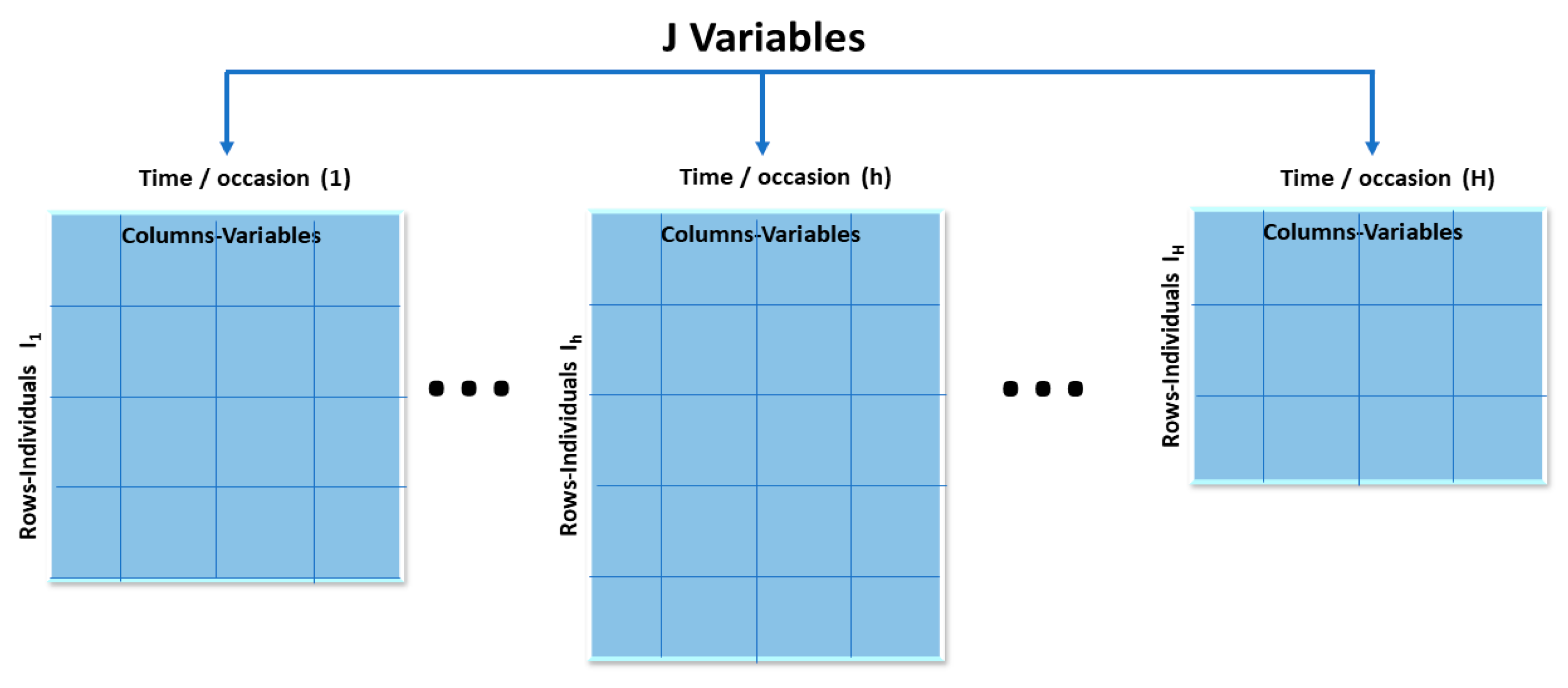
2.1. STATIS-Dual Method

The STATIS-dual is a methodology proposed by Escoufier and L’Hermier des Plantes [11,27], later Lavit [12], developed it extensively and Abdi et al. [15,28] explain it as a generalization of the principal components analysis (PCA) [29,30,31]. In any case, this method allows the simultaneous processing of several data tables.

In the STATIS-dual [11,32,33], the data correspond to a set of $H$ observations measured on the same set of variables. In this method, $H$ covariance matrices are calculated between the variables, one for each set of observations, a compromise map is provided for the variables, and partial loads for each table [34,35].

The scalar products between correlation matrices define a configuration of several points, in which each one of them represents one of the matrices (point clouds) [36]. The purpose is to find a compromise matrix, close to all the correlation matrices. This is defined as a weighted average of these matrices, being, therefore, a correlation matrix [37].

Given the compromise matrix, a series of results are generated in the form of point clouds that will be explored graphically, through factorial planes that do not necessarily pass through the center of gravity of the cloud [38]. The weighting that this method sometimes uses does not balance the influence of the different tables, but rather assigns greater weight to those that present a structure similar to the common structure, penalizing, in a certain sense, the rest [39,40].

The STATIS-dual method considers the $H$ tables $Y_1,\dots , Y_h,\dots , Y_H$ with $I_1, \dots , I_H$ observations and $J$ variables; each of these represents different scenarios or moments (Figure 1). Like standard STATIS, tables must be pre-processed using methods such as centering, scaling, and/or normalization of data, as indicated by Abdi et al. [15] and Marcondes Filho, de Oliveira & Fogliatto [41] among others.

The STATIS-dual method allows representing data matrices corresponding to the different occasions as points in a low-dimensional vector space, which is achieved using the covariance matrices [42].

In the resulting Euclidean image, the distance between points is interpreted in terms of similarity and, therefore, in the similarity between the variance–covariance structure and the congruence between factorial structures. The structures will be similar if the angles formed by the vectors of the Euclidean image approach zero [43].

2.2. STATIS-Dual Steps

The first step is the interstructure analysis, whereby the relationship between the different matrices is studied. The purpose is to find a matrix of vector correlations [44] between matrices; in other words, the global differentiation between data tables. The purpose is to analyze configurations of the $H$ points that correspond to the $H$ matrices in the graphic representation of one or more Euclidean images in the plane of the projection of the $H$ points.

To this end, the interstructure is represented in a reduced-dimensional subspace, spectrally decomposing the matrix of vector correlations and projecting it [28].

The object that each matrix represents is defined, a metric is chosen in the space of the objects, and a Euclidean image of said matrices is determined, associated with the scalar products introduced in the previous stage. The proximity between two points corresponds to the similarity (with respect to the distance considered) between the matrices corresponding to those points [45].

In this way, we obtain the $H$ preprocessed matrices ${Y^{\prime }}_1,\dots , {Y^{\prime }}_H$ each with dimension $I_h\times J$. These matrices are stacked vertically to structure the matrix ${Y^{\prime }}_{I\times J}$where $I=I_1+\dots +I_H$. For each table ${Y^{\prime }}_h$ a matrix $J\times J$ of cross products is obtained, as follows:

$$S_h={Y^{\prime }}_h^T{Y^{\prime }}_h$$

(1)

Each symmetric matrix of cross products $S_h$ is vectorized. The vectors obtained are stored in a new matrix $W_{H\times J^2}$ [46,47].

The matrix $A_{H\times H}$ is calculated from the matrix $W{W}^T$. This positive semi-definite matrix allows us to represent each of the H tables in the plane by decomposing the eigenvalues, considering that the eigenvalues are ordered from highest to lowest, we have:

$$A=U\mathsf{\Delta }{U}^T$$

(2)

where$U$ is a matrix that includes the eigenvectors of $A$ and $\mathsf{\Delta }$ is a diagonal matrix containing the corresponding eigenvalues (Figure 2).

An optional way to calculate $U$ is to perform a singular value decomposition (SVD) [48] of the matrix $W$:

$$W=U\Theta V^T$$

(3)

with

$${\Theta }^2=\Delta$$

(4)

Let the rank of the matrix $W$, $U_{H\times L}$ be the matrix that contains the left singular vectors of $W$, $\Theta$ a diagonal matrix of $L\times L$ containing the singular values of $W$, and $V$ contains the right singular vectors of $W$ in a matrix $J^2\times L$.

The SVD of $A$ allows the tables to be represented as points in the plane, called interstructure space, using the first and second columns of the matrix $U$ as coordinates:

$${\rm Z}=U\Theta =WV$$

(5)

The second step is the analysis of the compromise, where first a mass, called ${\alpha }_j$, is fixed to each variable. Masses are non-negative elements whose sum is equal to one [49]. Different masses can be calculated for each variable; however, equal masses are often chosen to ensure that all variables are equally important to the analysis [15,37]. A diagonal matrix $D^{\prime }$ is obtained for the masses of the variables, dividing the identity matrix$I_{J\times J}$ by the$J$ variables

$$D’=\frac{I_{J\times J}}{J}$$

(6)

Now the triplet ($Y^{\prime };M;D^{\prime })$is made up of preprocessed tables, the weights and masses [28].

3. Sparse STATIS-Dual

The selection and reduction in variables in multidimensional data is a subject with a long history within multivariate analysis. Some researchers have dedicated efforts to present alternatives that provide solutions to the problems of the high dimensionality of three-way data with regularization techniques, specifically in the PARAFAC/CANDECOMP techniques [50,51]. In particular, in the case of STATIS-dual, no studies have been found for the solution to this issue. In this sense, our proposal applies a regularization method through the elastic net Zou & Hastie method [52], which integrates the Ridge [53] and LASSO [54] regularization methods. This regularization method penalizes the size of the regression coefficients based on the$L_1$ y $L_2$norms.

One of the most important components of the elastic net method are the estimated coefficients ${\widehat{\theta }}^{elasticnet}$, which are the values that:

$${\widehat{\theta }}^{elasticnet}=\Vert {\upsilon }_i-W\theta {\Vert }^2+{\omega }_2{\displaystyle \sum }_{j=1}^p{\theta }_j^2+{\omega }_1{\displaystyle \sum }_{j=1}^p\left|{\theta }_j\right|$$

(7)

where ${\omega }_1$ > 0 and ${\omega }_2$ > 0 are complexity parameters.

Thus, we have the term ${\omega }_1{\displaystyle \sum }_{j=1}^p\left|{\theta }_j\right|$ which points to sparse solutions. At the same time, the term ${\omega }_2{\displaystyle \sum }_{j=1}^p{\theta }_j^2$indicates that highly correlated predictors achieve similar estimated coefficients [23].

Similarly, it is considered,

$${\widehat{\theta }}^{elasticnet}=arg min \Vert {\upsilon }_i-W\theta {\Vert }^2$$

(8)

conditioned to ${\displaystyle \sum }_{j=1}^p{\theta }_j^2\le \omega y{\displaystyle \sum }_{j=1}^p\left|{\theta }_j\right|\le \omega$.

Based on this condition, Zou & Hastie [52] propose to construct the new$\theta$ by means of the following formula:

$$V^{soft}=sign\left(V\right)\frac{{(\left|V-{\omega }_1\right|)}_{+}}{1+{\omega }_2 }$$

(9)

where the $L_1$ and $L_2$ standards are integrated, applying the soft-thresholding operator.

The elastic net regularization can be implemented in the STATIS-dual, adjusting LASSO and Ridge to derive modified loads. For this, the model is used:

$$W=Q{\mathsf{\Lambda }}^{\frac{1}{2}}+E$$

(10)

With this method modified loads are derived for the STATIS-dual, of the form:

$$V_{elasticnet}=argmin \Vert W-Q{\mathsf{\Lambda }}^{1/2}{\Vert }^2+{\omega }_2{\displaystyle \sum }_{j=1}^p{V}_j^2+{\omega }_1{\displaystyle \sum }_{j=1}^p\left|V_j\right|$$

(11)

where ${\omega }_1$ is the LASSO penalty parameter to promote sparsity and ${\omega }_2$ is the regularization parameter to reduce loads.

Now, taking into account the first k factorial axes, the matrices are defined ${\Phi }_{pxk}=\left[{\phi }_1, {\phi }_2,\dots , {\phi }_k\right]$.

For some${\omega }_2>0,$ let:

$$\left(\widehat{\Phi },\widehat{\Theta }\right)=argmin {\displaystyle \sum }_{i=1}^n\Vert w_i-\Phi {\Theta }^T{w}_i{\Vert }^2+{\omega }_2{\displaystyle \sum }_{j=1}^k\Vert {\theta }_j{\Vert }^2+{\omega }_{1,j}{\displaystyle \sum }_{j=1}^k\Vert {\theta }_j{\Vert }_1$$

(12)

conditioned to ${\Phi }^T\Phi =I_{KxK}$. Then ${\widehat{\theta }}_j\propto V_j\mathrm{for}j=1,2,\dots ,k$.

Considering that

$${\displaystyle \sum }_{i=1}^n\Vert w_i-\Phi {\Theta }^T{w}_i{\Vert }^2=\Vert W-W\Theta {\Phi }^T{\Vert }^2=\Vert W\Phi {\Vert }^2+\Vert W\Phi -W\Theta {\Vert }^2=\Vert W\Phi {\Vert }^2+{\displaystyle \sum }_{j=1}^k\Vert W{\phi }_j-W{\theta }_j{\Vert }^2$$

(13)

The solution is obtained by alternating optimization on $\Phi$ and $\Theta$ using the LARS-EN algorithm [52].

Given fixed$\Phi$ we have:

$${\widehat{\theta }}_j=argmin \Vert W{\phi }_j-W{\theta }_j{\Vert }^2+{\omega }_2\Vert {\theta }_j{\Vert }^2+{\omega }_{1,j}\Vert {\theta }_j{\Vert }_1={({\phi }_j-{\theta }_j)}^T{W}^{T}W\left({\phi }_j-{\theta }_j\right)+{\omega }_2\Vert {\beta }_j{\Vert }^2+{\omega }_{1,j}\Vert {\theta }_j{\Vert }_1$$

(14)

Therefore, each ${\widehat{\theta }}_j$ is an elastic net estimator.

With $\Theta$ fixed, the penalty part is not taken into account and is minimized:

$$arg min{{\displaystyle \sum }}_{i=1}^n\Vert w_i-\Phi {\Theta }^T{w}_i{\Vert }^2=\Vert W-W\Theta {\Phi }^T{\Vert }^2\mathrm{conditioned}\mathrm{to}{\Phi }^T\Phi =I_{KxK}$$

(15)

This leads to a Procrustes problem [55], and the solution is supplied by the $DVS(W^{T}W)\Theta =UD{V}^T$ and $\widehat{\Phi }=U{V}^T$ is determined.

In summary, elastic net contemplates the following: (1) it uses the $L_1$ and $L_2$ norms; (2) selects variables; (3) penalizes charges; and (4) contracts some charges towards zero, and cancels other charges. There are no obvious and determined methods to adjust the parameters ${\omega }_1$ and ${\omega }_2$. It is proposed to test various combinations and choose the one that provides a balance between the explained variance and the sparsity, giving preponderance to the variance.

The variable projection method [56] is proposed as another solution to the optimization problem.

The steps for the implementation of the elastic net regularization method in STATIS-dual are presented in Algorithm 1:

Algorithm 1. Sparse STATIS-Dual.

Step 1. Consider an array of data nxp. Step 2. A tolerance value is set (1 × 10−5). Step 3. The data are transformed (center or standardize). Step 4. Matrices of cross products $S_h$ are obtained.Step 5. The cosine matrix between studies $C$ is obtained. Step 6. A PCA is performed on $C$. Step 7. The compromise matrix$S$ is obtained. Step 8. The decomposition in SVD of the compromise matrix is carried out. Step 9. We take $\Phi$as the charges of the first m components $V\left[,1:n\right]$. Step 10. ${\theta }_j$ is calculated by: $${\theta }_j={({\phi }_j-{\theta }_j)}^T{W}^{T}W\left({\phi }_j-{\theta }_j\right)+{\omega }_2\Vert {\theta }_j{\Vert }^2+{\omega }_{1,j}\Vert {\theta }_j{\Vert }_1$$ Step 11. $\Phi$ is updated by the SVD of $W^{T}W\theta$: $$W^{T}W\theta =UD{V}^T\to \Phi =U{V}^T$$ Step 12. The difference between $\Phi$ and $\Theta$ is updated. $$di{f}_{\Phi \Theta }=\frac{1}{p}{\displaystyle \sum }_{i=1}^p\frac{1}{{\left|{\theta }_i\right|}^2{\left|\phi \right|}^2}{\displaystyle \sum }_{j=1}^m{\theta }_{ij}-{\phi }_{ij}$$ Step 13. Steps 4, 5 and 6 are repeated until $dif \Phi \Theta$ < tolerance. Step 14. The columns ${\widehat{V}}_J^{EN}=\frac{{\theta }_j}{\Vert {\theta }_j\Vert },j=1,\dots ,n$, are normalized. Step 15. The restricted loads are obtained to project the variables in the compromise. Step 16. The STATIS-dual Sparse obtained through the previous steps is plotted.

Figure 3 shows the steps that describe the application of the penalty on the STATIS-dual, which leads to obtaining the modified load matrix.

In the interest of providing a tool that implements the algorithms described, a package has been created in the programming language R [57].

This package, called SparseSTATISdual [25], makes it possible to use the algorithm from different data sources and generate graphical and numerical results, both for the STATIS-dual and for the Sparse STATIS-dual.

The numerical results generated by this package are the following: pre-processed matrix, scalar product matrices, cosine matrix, interstructure, weights of each matrix, compromise matrix, factor load coefficients, and projection matrix. In addition to the interstructure, compromise and intrastructure graphs are used.

The main function of the package is the application of penalty measures to contract and select variables simultaneously. With this method, the obtained model offers results that allow a better interpretation.

4. Illustrative Example

In this section, we proceed to implement the new algorithm to the data set on innovation indicators, explained in Section 2. A comparison of results is made between the dual STATIS and the STATIS-dual Sparse to illustrate the performance of our algorithm and the advantage of its practical interpretation.

We first present the classic STATIS-dual analysis, followed by the results of the Sparse STATIS-dual. On a practical level, the objective of our new model is not to produce disjoint factors, but to achieve null coefficients that allow a correct interpretation of the results.

To analyze the indicators of global innovation during the 2016–2020 period, the STATIS-dual analysis begins evaluating the interstructure (Figure 4). The first main plane shows the global evolution of innovation in the indicated period, which explains 59% of the total inertia. In this figure, the vector correlations between the data tables (years) are visualized, clearly observing two scenarios; a first scenario that shows the high similarity between the years 2016, 2017, and 2018; and a second scenario consisting of the years 2019 and 2020. With this, it can be inferred that there has been a change in the innovation indicators between these two periods. The vectors that represent each year are very close to the circumference of radius one, which guarantees a good representation of the reality described by the data matrices.

Next, the compromise matrix is built that synthesizes the common structure of all the original matrices. By drawing the structure of the compromise matrix, we capture the multivariate nature of the data and represent the indicators under study.

Table 1. Compromise matrix weights.

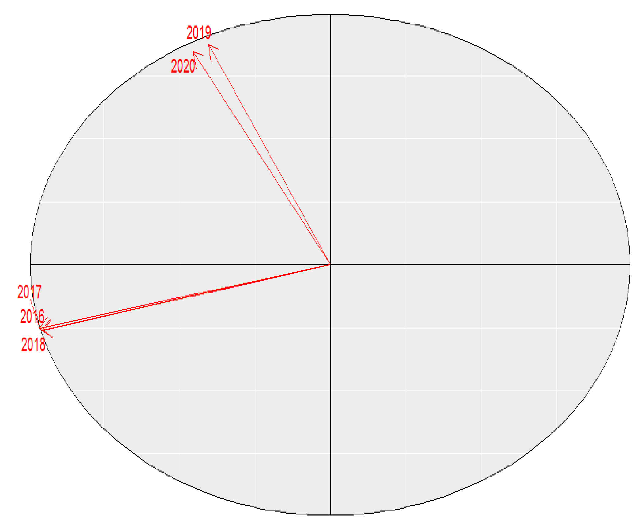
Axis	Weights
2016	0.3956
2017	0.3994
2018	0.3941
2019	0.1672
2020	0.1881

presents the weight that each matrix contributes to the construction of the compromise. As can be seen, the data tables for the years 2016–2018 contribute a greater weight to the construction of the compromise matrix and obtain a good representation in the subspace created. The last two years, 2019 and 2020, also contribute to the construction of the compromise matrix, but to a lesser extent. These weights show the vector correlations between periods, described in the interstructure.

Figure 5 presents the projection of the compromise matrix to explore the average of the innovation indicators in the study period. Although the most relevant indicators are represented in the first factorial axis, the high number of these (80 in total) makes their reading and interpretation confusing; thus, a reduction in indicators is necessary to allow us to identify those that most contribute to the interpretation of global innovation. Hence, the importance of incorporating regularization methods, consistent with large matrices, promotes the cancellation of factor loads with coefficients close to zero.

Similar to the three-way methods, the proposed Sparse STATIS-dual method is developed in three phases: interstructure, compromise matrix, and intrastructure.

Below is the representation of the Sparse STATIS-dual compromise (Figure 6). As can be seen, by incorporating the elastic net penalty, exactly zero coefficients were achieved, simplifying the interpretation of the results obtained.

Without prejudice to the other indicators related to innovation, the analysis using the Sparse STATIS-dual made it possible to understand which aspects have a greater contribution towards innovative results in world economies. The potential of our proposal is used to generate null coefficients in the load vectors.

Table 2. Loadings Matrix for the First Three Dimensions Obtained From STATIS-dual and Sparse STATIS-dual.

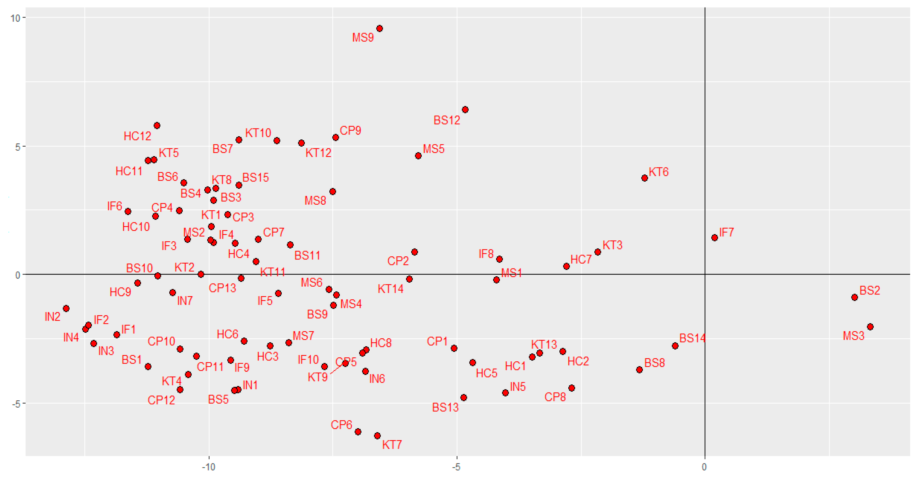
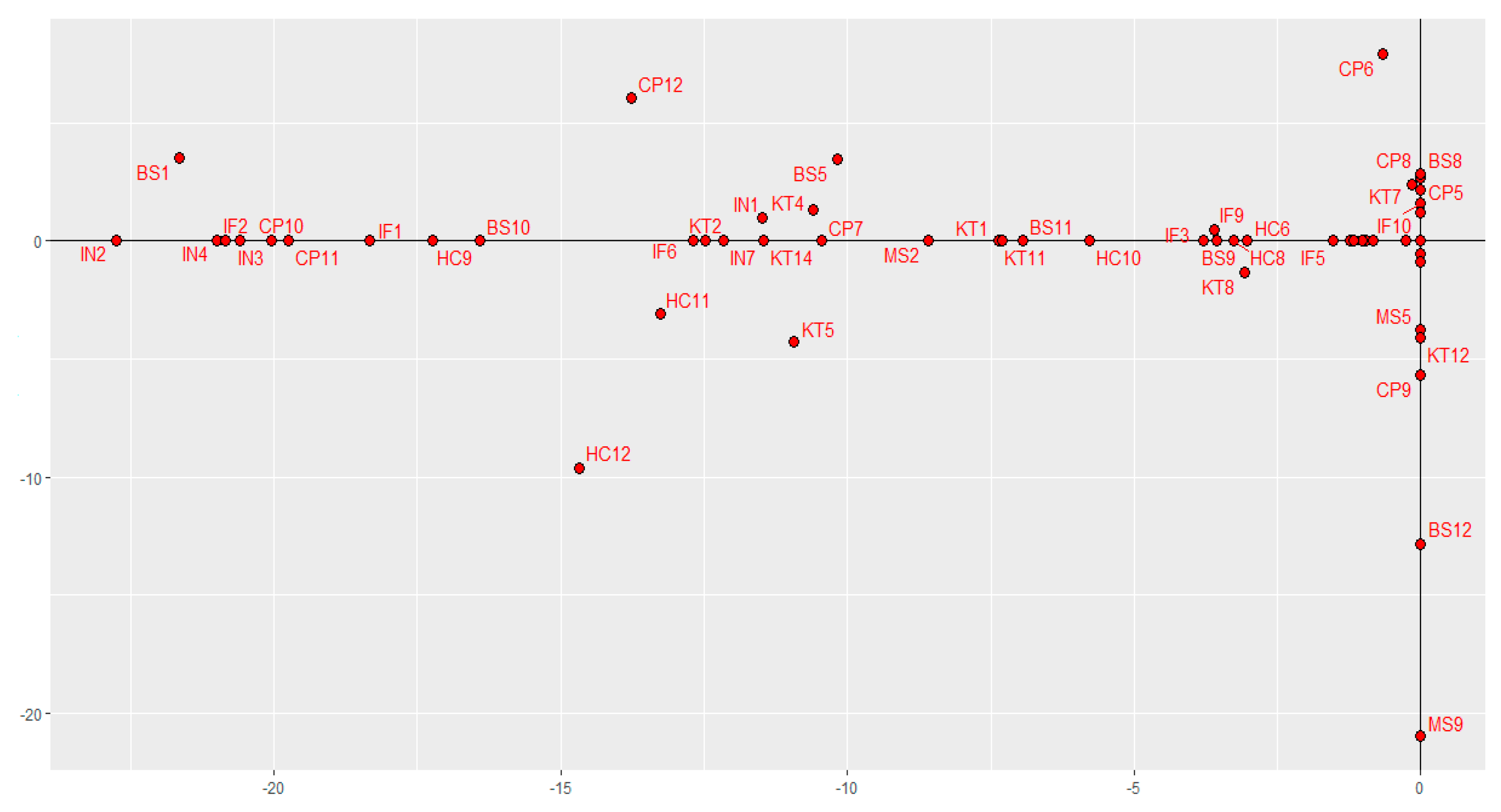
Indicators	STATIS-Dual			Sparse STATIS-Dual
	Axis 1	Axis 2	Axis 3	Axis 1	Axis 2	Axis 3
IN1	−9.407	−4.458	0.171	−11.496	0.958	0
IN2	−12.876	−1.326	−0.389	−22.754	0	0
IN3	−12.318	−2.665	−0.639	−20.605	0	0
IN4	−12.484	−2.132	−1.767	−20.992	0	0
IN5	−4.026	−4.586	−1.891	0	0	0
IN6	−6.850	−3.741	0.712	−0.969	0	0
IN7	−10.728	−0.710	1.185	−12.158	0	0
HC1	−3.481	−3.195	−0.607	0	0	0
HC2	−2.865	−2.996	−1.373	0	0	0
HC3	−8.772	−2.766	4.567	0	0	9.612
HC4	−9.469	1.214	−1.286	−0.266	0	0
HC5	−4.693	−3.414	4.649	0	0	3.718
HC6	−9.290	−2.582	6.100	−3.022	0	14.754
HC7	−2.803	0.316	3.349	0	0	5.670
HC8	−6.828	−2.935	−4.465	−3.267	0	−0.486
HC9	−11.442	−0.319	−2.178	−17.242	0	0
HC10	−11.081	2.269	−1.695	−5.776	0	0
HC11	−11.225	4.429	−1.061	−13.263	−3.114	0
HC12	−11.041	5.776	0.397	−14.666	−9.619	0
IF1	−11.859	−2.339	2.262	−18.329	0	0.239
IF2	−12.420	−1.966	1.659	−20.854	0	0
IF3	−10.434	1.375	3.590	−3.783	0	1.138
IF4	−9.901	1.247	4.421	0	0	3.205
IF5	−8.606	−0.725	−1.401	−1.525	0	0
IF6	−11.629	2.461	−0.939	−12.690	0	0
IF7	0.191	1.429	1.250	0	0	0
IF8	−4.145	0.592	−0.230	0	0	0
IF9	−9.568	−3.322	3.980	−3.609	0.462	4.520
IF10	−7.677	−3.558	6.018	0	1.566	8.599
MS1	−4.201	−0.216	3.565	0	0	0
MS2	−9.960	1.334	−0.915	−8.587	0	0
MS3	3.327	−2.018	1.068	0	0	0
MS4	−7.436	−0.783	2.959	0	0	0.237
MS5	−5.774	4.606	−4.881	0	−3.755	−5.575
MS6	−7.587	−0.569	−6.428	−1.185	0	−6.019
MS7	−8.395	−2.652	2.479	−0.832	0	0
MS8	−7.511	3.223	0.710	0	0	0
MS9	−6.558	9.565	3.786	0	−20.989	0
BS1	−11.226	−3.558	0.899	−21.651	3.505	0
BS2	3.009	−0.892	6.874	0	0	1.667
BS3	−9.907	2.885	−2.446	−1.032	0	−2.004
BS4	−10.032	3.291	0.352	0	0	0
BS5	−9.483	−4.497	3.686	−10.185	3.437	2.683
BS6	−10.513	3.552	−2.799	−1.244	0	0
BS7	−9.400	5.219	−2.592	0	−0.551	0
BS8	−1.327	−3.702	−1.609	0	2.673	0
BS9	−7.488	−1.205	−5.744	−3.558	0	−4.372
BS10	−11.026	−0.062	−3.100	−16.404	0	−0.797
BS11	−8.365	1.145	−0.748	−6.938	0	0
BS12	−4.837	6.407	3.225	0	−12.855	0
BS13	−4.864	−4.774	−4.248	0	0	0
BS14	−0.612	−2.777	−3.615	0	0	−5.485
BS15	−9.403	3.468	−2.028	0	0	−0.856
KT1	−9.955	1.870	0.468	−7.369	0	0
KT2	−10.164	0.004	−2.983	−12.489	0	−1.787
KT3	−2.164	0.883	5.046	0	0	0
KT4	−10.422	−3.882	0.282	−10.594	1.2813	0
KT5	−11.100	4.453	0.386	−10.928	−4.2657	0
KT6	−1.226	3.740	−0.109	0	0	0
KT7	−6.606	−6.269	−0.608	−0.164	2.363	0
KT8	−9.858	3.351	−0.238	−3.083	−1.333	0
KT9	−7.257	−3.439	6.139	0	1.189	9.004
KT10	−8.638	5.197	1.039	0	−0.883	0
KT11	−9.057	0.498	−3.782	−7.295	0	−3.882
KT12	−8.141	5.118	3.562	0	−4.118	−0.215
KT13	−3.332	−3.059	−2.231	0	0	0
KT14	−5.959	−0.173	−2.480	−11.464	0	−0.857
CP1	−5.059	−2.849	4.737	0	0	0
CP2	−5.852	0.891	3.246	0	0	0
CP3	−9.621	2.315	−0.623	0	0	0
CP4	−10.598	2.492	−0.640	0	0	0
CP5	−6.902	−3.051	−0.116	0	2.161	0
CP6	−6.999	−6.115	−1.789	−0.657	7.923	0
CP7	−9.002	1.380	−5.604	−10.456	0	−1.136
CP8	−2.694	−4.406	−1.410	0	2.859	0
CP9	−7.449	5.332	5.023	0	−5.683	0
CP10	−10.576	−2.898	−3.105	−20.054	0	0
CP11	−10.249	−3.175	−0.456	−19.742	0	0
CP12	−10.576	−4.470	0.979	−13.762	6.030	0
CP13	−9.352	−0.128	−1.566	−1.162	0	0

shows the coefficients of the load matrix associated with the factorial axes in the first three dimensions—both for the STATIS-dual and the Sparse STATIS-dual. These results serve to compare the contributions of the innovation indicators to the factorial axes. As can be seen, in the STATIS-dual each factorial axis is obtained as a linear combination of all the indicators, which makes it difficult to describe each axis. On the contrary, the Sparse STATIS-dual leads to obtaining coefficients with exactly zero values, so that the interpretation of the axes depends only on a subset of innovation indicators, the most relevant ones. According to the configuration of the indicators in each dimension, the axes are labeled as follows: research, education, and efficient government (axis 1); competitive market (axis 2); and quality management (axis 3).

5. Conclusions and Discussion

One of the most important areas of current research in multivariate data analysis focuses on the development of efficient techniques for the study of large data matrices [22,58,59].

In this article, a new technical contribution to three-way data analysis is developed using the elastic net regularization method. The advantage of this method, which combines the properties of ridge and lasso regularization, consists mainly in the selection of the most relevant variables, providing efficient solutions when studying multidimensional data [24] or data sets in which the number of observations is greater than the number of variables.

This new methodology, called Sparse STATIS-dual, provides a holistic understanding of the three-way data structure, facilitating the interpretation of the results. To support the new Sparse STATIS-dual method, a package is implemented in the R programming language [25]. The package, called Sparse STATIS-dual, allows us to implement our theoretical proposal, facilitating its application to any three-way data set.

Very few studies have evidenced the use of sparse penalties in three-way data. Recently, an extension of the three-way Tucker models has been formulated and the C_enetTucker models have been proposed to produce sparse component arrays [14]. Therefore, our contribution opens up the doors for the research and development of new applications sparse in other techniques of the STATIS family or the multivariate analysis of three-way data.

References

- Cuadras, C.M. Nuevos Métodos de Análisis Multivariante; CMC Edicions: Barcelona, Spain, 1996. [Google Scholar]
- Gabriel, K.R. The biplot graphic display of matrices with application to principal component analysis. Biometrika 1971, 58, 453–467. [Google Scholar] [CrossRef]
- Gabriel, K.R.; Odoroff, C.L. Biplots in biomedical research. Stat. Med. 1990, 9, 469–485. [Google Scholar] [CrossRef] [PubMed]
- Tucker, L.R. Some mathematical notes on three-mode factor analysis. Psychometrika 1966, 31, 279–311. [Google Scholar] [CrossRef]
- Geladi, P. Analysis of multi-way (multi-mode) data. Chemom. Intell. Lab. Syst. 1989, 7, 11–30. [Google Scholar] [CrossRef]
- Carroll, J.D.; Arabie, P. Multidimensional Scaling. Annu. Rev. Psychol. 1980, 31, 607–649. [Google Scholar] [CrossRef]
- Kiers, H.A.L. Comparison of“anglo-saxon” and “french” three-mode methods. Stat. Anal. Données 1988, 13, 14–32. [Google Scholar]
- Kiers, H.A.L. Hierarchical relations among three-way methods. Psychometrika 1991, 56, 449–470. [Google Scholar] [CrossRef]
- Kroonenberg, P.M. Three-mode component models: A review of the literature. Stat. Appl. 1992, 4, 619–633. [Google Scholar]
- Escoufier, Y. L’analyse conjointe de plusieurs matrices de données. In Biométrie et Temps; Jolivet, M., Ed.; Société Française de Biométrie: Paris, France, 1980; pp. 59–76. [Google Scholar]
- L’Hermier des Plantes, H. Structuration des Tableaux à Trois Indices de la Statistique; Université de Montpellier II: Montpellier, France, 1976. [Google Scholar]
- Lavit, C. Analyse Conjointe de Tableaux Quantitatifs; Masson: Paris, France, 1988; ISBN 2225814783. [Google Scholar]
- Lavit, C.; Escoufier, Y.; Sabatier, R.; Traissac, P. The ACT (STATIS method). Comput. Stat. Data Anal. 1994, 18, 97–119. [Google Scholar] [CrossRef]
- González-García, N. Análisis Sparse de Tensores Multidimensionales; Universidad de Salamanca: Salamanca, Spain, 2019. [Google Scholar]
- Abdi, H.; Williams, L.J.; Valentin, D.; Bennani-Dosse, M. STATIS and DISTATIS: Optimum multitable principal component analysis and three way metric multidimensional scaling. WIREs Comput. Stat. 2012, 4, 124–167. [Google Scholar] [CrossRef]
- Llobell, F.; Cariou, V.; Vigneau, E.; Labenne, A.; Qannari, E.M. Analysis and clustering of multiblock datasets by means of the STATIS and CLUSTATIS methods. Application to sensometrics. Food Qual. Prefer. 2020, 79, 103520. [Google Scholar] [CrossRef]
- Llobell, F.; Vigneau, E.; Qannari, E.M. Clustering datasets by means of CLUSTATIS with identification of atypical datasets. Application to sensometrics. Food Qual. Prefer. 2019, 75, 97–104. [Google Scholar] [CrossRef]
- Fournier, M.; Motelay-Massei, A.; Massei, N.; Aubert, M.; Bakalowicz, M.; Dupont, J.P. Investigation of transport processes inside karst aquifer by means of STATIS. Ground Water 2009, 47, 391–400. [Google Scholar] [CrossRef] [PubMed]
- Chaya, C.; Perez-Hugalde, C.; Judez, L.; Wee, C.S.; Guinard, J.-X. Use of the STATIS method to analyze time-intensity profiling data. Food Qual. Prefer. 2003, 15, 3–12. [Google Scholar] [CrossRef]
- Stanimirova, I.; Walczak, B.; Massart, D.L.; Simeonov, V.; Saby, C.A.; Di Crescenzo, E. STATIS, a three-way method for data analysis. Application to environmental data. Chemom. Intell. Lab. Syst. 2004, 73, 219–233. [Google Scholar] [CrossRef]
- Coquet, R.; Troxler, L.; Wipff, G. The STATIS method: Characterization of conformational states of flexible molecules from molecular dynamics simulations in solution. J. Mol. Graph. 1996, 14, 206–212. [Google Scholar] [CrossRef]
- Rodríguez-Martínez, C.C. Contribuciones a los Métodos STATIS Basados en Técnicas de Aprendizaje no Supervisado; Universidad de Salamanca. Ph.D. Thesis, Universidad de Salamanca, Salamanca, Spain, 2020. [Google Scholar]
- Zou, H.; Hastie, T.; Tibshirani, R. Sparse Principal Component Analysis. J. Comput. Graph. Stat. 2006, 15, 265–286. [Google Scholar] [CrossRef]
- Cubilla-Montilla, M.; Nieto-Librero, A.B.; Galindo-Villardón, P.; Torres-Cubilla, C.A. Sparse HJ Biplot: A New Methodology via Elastic Net. Mathematics 2021, 9, 1298. [Google Scholar] [CrossRef]
- Rodríguez-Martínez, C.C.; Cubilla-Montilla, M. SparseSTATISdual: R package for penalized STATIS-dual análisis. Available online: https://github.com/CCRM07/SparseSTATISdual (accessed on 15 June 2021).
- Global Innovation Index. Available online: https://www.globalinnovationindex.org/analysis-indicator (accessed on 10 April 2021).
- Escoufier, Y. Objectifs et procédures de l’analyse conjointe de plusieurs tableaux de donnés. Stat. Anal. Données 1985, 10, 1–10. [Google Scholar]
- Abdi, H.; Valentin, D. DISTATIS How to analyze multiple distance matrices. In Encyclopedia of Measurement and Statistics; SAGE Publications, Inc.: Thousand Oaks, CA, USA, 2007; Volume 3. [Google Scholar]
- Hotelling, H. Analysis of a complex of statistical variables into principal components. J. Educ. Psychol. 1933, 24, 417. [Google Scholar] [CrossRef]
- Jolliffe, I.T. Principal Component Analysis, 2nd ed.; Springer: New York, NY, USA, 2002. [Google Scholar]
- Pearson, K. On lines and planes of closest fit to systems of points in space. Lond. Edinb. Dublin Philos. Mag. J. Sci. 1901, 2, 559–572. [Google Scholar] [CrossRef]
- Ambapour, S. Statis: Une méthode d’analyse conjointe de plusieurs tableaux de données, Document de travail (DT 01/2001), Bureau d’Application des Methodes Statistiques et Informatiques. 2001, pp. 1–20. Available online: https://www.yumpu.com/fr/document/read/37543574/statis-une-macthode-danalyse-conjointe-de-plusieurs-cnsee (accessed on 15 June 2021).
- L’Hermier des Plantes, H.; Thiébaut, B. Étude de la pluviosité au moyen de la méthode STATIS. Rev. Stat. Appl. 1977, 25, 57–81. [Google Scholar]
- Kroonenberg, P.M. Applied Multiway Data Analysis; Wiley Series in Probabity and Statistics; John Wiley & Sons, Inc.: New York, NY, USA, 2008; ISBN 978-0-470-16497-6. [Google Scholar]
- Niang, N.; Fogliatto, F.; Saporta, G. Contrôle multivarié de procédés par lots à l’aide de Statis. In Proceedings of the 41èmes Journée de Statistique, Nice, France, 25–29 May 2009. [Google Scholar]
- Lekve, K. Species richness and environmental conditions of fish along the Norwegian Skagerrak coast. ICES J. Mar. Sci. 2002, 59, 757–769. [Google Scholar] [CrossRef]
- Lobry, J.; Lepage, M.; Rochard, E. From seasonal patterns to a reference situation in an estuarine environment: Example of the small fish and shrimp fauna of the Gironde estuary (SW France). Estuar. Coast. Shelf Sci. 2006, 70, 239–250. [Google Scholar] [CrossRef]
- da Silva, J.L.; Ramos, L.P. On the rate of convergence of uniform approximations for sequences of distribution functions. J. Korean Stat. Soc. 2014, 43, 47–65. [Google Scholar] [CrossRef]
- Ferraro, S.; Ardoino, I.; Bassani, N.; Santagostino, M.; Rossi, L.; Biganzoli, E.; Bongo, A.S.; Panteghini, M. Multi-marker network in ST-elevation myocardial infarction patients undergoing primary percutaneous coronary intervention: When and what to measure. Clin. Chim. Acta 2013, 417, 1–7. [Google Scholar] [CrossRef] [PubMed]
- Caballero-Juliá, D.; Galindo-Villardón, P.; García, M.-C. JK-Meta-Biplot y STATIS Dual como herramientas de análisis de tablas textuales múltiples. RISTI Rev. Ibérica Sist. Tecnol. Inf. 2017, 25, 18–33. [Google Scholar] [CrossRef][Green Version]
- Marcondes Filho, D.; de Oliveira, L.P.L.; Fogliatto, F.S. Erratum to: Multivariate quality control of batch processes using STATIS. Int. J. Adv. Manuf. Technol. 2017, 88, 2355. [Google Scholar] [CrossRef]
- Enachescu, C.; Postelnicu, T. Patterns in journal citation data revealed by exploratory multivariate analysis. Scientometrics 2003, 56, 43–59. [Google Scholar] [CrossRef]
- Ramos-Barberán, M.; Hinojosa-Ramos, M.V.; Ascencio-Moreno, J.; Vera, F.; Ruiz-Barzola, O.; Galindo-Villardón, P. Batch process control and monitoring: A Dual STATIS and Parallel Coordinates (DS-PC) approach. Prod. Manuf. Res. 2018, 6, 470–493. [Google Scholar] [CrossRef]
- Robert, P.; Escoufier, Y. A Unifying Tool for Linear Multivariate Statistical Methods: The RV-Coefficient. Appl. Stat. 1976, 25, 257. [Google Scholar] [CrossRef]
- Lebart, L.; Morineau, A.; Piron, M. Statistique Exploratoire Multidimensionnelle; Dunod: Paris, France, 1995. [Google Scholar]
- Oliveira, M.M.; Mexia, J. ANOVA-like analysis of matched series of studies with a common structure. J. Stat. Plan. Inference 2007, 137, 1862–1870. [Google Scholar] [CrossRef]
- Vicente-Galindo, P.; Galindo-Villardón, P. El método Statis como alternativa para detectar” response shift” en estudios de calidad de vida relacionada con la salud. Revista de Matemática: Teoría y Aplicaciones 2009, 16, 1–15. [Google Scholar] [CrossRef][Green Version]
- Eckart, C.; Young, G. The approximation of one matrix by another of lower rank. Psychometrika 1936, 1, 211–218. [Google Scholar] [CrossRef]
- Castillo Elizondo, W.; González Varela, J. STATIS DUAL: Software y Análisis de datos reales. Revista de Matemática: Teoría y Aplicaciones 1998, 5, 149–162. [Google Scholar]
- Giordani, P.; Rocci, R. Constrained CANDECOMP/PARAFAC via the Lasso. Psychomotrika 2013, 78, 669–685. [Google Scholar] [CrossRef] [PubMed]
- Giordani, P.; Rocci, R. Candecomp/Parafac with ridge regularization. Chemom. Intell. Lab. Syst. 2013, 129, 3–9. [Google Scholar] [CrossRef]
- Zou, H.; Hastie, T. Regularization and variable selection via the elastic net. J. R. Stat. Soc. 2005, 67, 301–320. [Google Scholar] [CrossRef]
- Hoerl, A.E.; Kennard, R.W. Ridge Regression: Biased Estimation for Nonorthogonal Problems. Technometrics 1970, 12, 55–67. [Google Scholar] [CrossRef]
- Tibshirani, R. Regression Shrinkage and Selection Via the Lasso. J. R. Stat. Soc. Ser. B 1996, 58, 267–288. [Google Scholar] [CrossRef]
- Gower, J.C. Procrustes Analysis. In International Encyclopedia of the Social & Behavioral Sciences, 2nd ed.; Elsevier: Amsterdam, The Netherlands, 2015; ISBN 9780080970875. [Google Scholar]
- Erichson, N.B.; Zheng, P.; Manohar, K.; Brunton, S.L.; Kutz, J.N.; Aravkin, A.Y. Sparse Principal Component Analysis via Variable Projection. SIAM J. Appl. Math. 2020, 80, 977–1002. [Google Scholar] [CrossRef]
- R Development Core Team R Software. R: A Language and Environment Statistical Computing; R Foundation for Statical Computing: Vienna, Austria; Available online: https://www.R-project.org/ (accessed on 15 June 2021).
- Grané, A.; Sow-Barry, A.A. Visualizing Profiles of Large Datasets of Weighted and Mixed Data. Mathematics 2021, 9, 891. [Google Scholar] [CrossRef]
- Laria, J.C.; Aguilera-Morillo, M.C.; Álvarez, E.; Lillo, R.E.; López-Taruella, S.; del Monte-Millán, M.; Picornell, A.C.; Martín, M.; Romo, J. Iterative Variable Selection for High-Dimensional Data: Prediction of Pathological Response in Triple-Negative Breast Cancer. Mathematics 2021, 9, 222. [Google Scholar] [CrossRef]